Testing neural network intelligence using Raven’s

Comenius University in Bratislava

Faculty of Mathematics, Physics and Informatics

Testing neural network intelligenceusing Raven’s Progressive Matrices

Bachelor Thesis

2021Nina Raganová

ii

Comenius University in Bratislava

Faculty of Mathematics, Physics and Informatics

Testing neural network intelligenceusing Raven’s Progressive Matrices

Bachelor Thesis

Study Programme: Computer ScienceField of Study: Computer ScienceDepartment: Department of Applied InformaticsSupervisor: prof. Ing. Igor Farkaš, Dr.

Bratislava, 2021Nina Raganová

iv

Univerzita Komenského v BratislaveFakulta matematiky, fyziky a informatiky

ZADANIE ZÁVEREČNEJ PRÁCE

Meno a priezvisko študenta: Nina RaganováŠtudijný program: informatika (Jednoodborové štúdium, bakalársky I. st., denná

forma)Študijný odbor: informatikaTyp záverečnej práce: bakalárskaJazyk záverečnej práce: anglickýSekundárny jazyk: slovenský

Názov: Testing neural network intelligence using Raven’s Progressive MatricesTestovanie inteligencie neurónovej siete použitím Ravensových progresívnychmatíc

Anotácia: Ravensove progresívne matice (RPM) sa často používajú na testovanie IQu ľudí, a to ako miera abstraktného uvažovania prostredníctvom neverbálnychotázok. V umelej inteligencii je jedným z najdôležitejších cieľov výroba strojovs rozumovou schopnosťou podobnou ľudskej, aby boli užitočné pre rôzne úlohy.Najsľubnejší prístup je založený na umelých neurónových sieťach.

Cieľ: 1. Implementujte vybranú neurónovú sieť a trénujte ju na riešenie problémuRPM.2. Otestujte úspešnosť modelu v rôznych scenároch týkajúcich sa variabilitya veľkosti trénovacej množiny.3. Interpretujte získané výsledky.

Literatúra: Zhuo T., Kankanhalli M. (2020). Solving Raven’s Progressive Matrices withNeural Networks. https://arxiv.org/pdf/2002.01646Jahrens M., Martinetz T. (2020). Solving Raven’s Progressive Matrices withMulti-Layer Relation Networks. https://arxiv.org/pdf/2003.11608Zhang C. et al. (2019). Raven: A dataset for relational and analogical visualreasoning. In CVPR, https://arxiv.org/pdf/1903.02741

Vedúci: prof. Ing. Igor Farkaš, Dr.Katedra: FMFI.KAI - Katedra aplikovanej informatikyVedúci katedry: prof. Ing. Igor Farkaš, Dr.

Dátum zadania: 28.10.2020

Dátum schválenia: 31.10.2020 doc. RNDr. Daniel Olejár, PhD.garant študijného programu

študent vedúci práce

vi

Comenius University in BratislavaFaculty of Mathematics, Physics and Informatics

THESIS ASSIGNMENT

Name and Surname: Nina RaganováStudy programme: Computer Science (Single degree study, bachelor I. deg., full

time form)Field of Study: Computer ScienceType of Thesis: Bachelor´s thesisLanguage of Thesis: EnglishSecondary language: Slovak

Title: Testing neural network intelligence using Raven’s Progressive Matrices

Annotation: Raven’s Progressive Matrices (RPM) have been widely used for IQ testingin humans, namely as a measure of abstract reasoning through non-verbalquestions. In AI, one of the most important goals is to make machines withreasoning ability similar to that of humans in order to make them usefulfor various tasks. The most promising approach is based on artificial neuralnetworks.

Aim: 1. Implement a chosen neural network and train it for solving the RPM problem.2. Test the model performance in various scenarios concerning the variabilityand the size of the training set.3. Interpret obtained results.

Literature: Zhuo T., Kankanhalli M. (2020). Solving Raven’s Progressive Matrices withNeural Networks. https://arxiv.org/pdf/2002.01646Jahrens M., Martinetz T. (2020). Solving Raven’s Progressive Matrices withMulti-Layer Relation Networks. https://arxiv.org/pdf/2003.11608Zhang C. et al. (2019). Raven: A dataset for relational and analogical visualreasoning. In CVPR, https://arxiv.org/pdf/1903.02741

Supervisor: prof. Ing. Igor Farkaš, Dr.Department: FMFI.KAI - Department of Applied InformaticsHead ofdepartment:

prof. Ing. Igor Farkaš, Dr.

Assigned: 28.10.2020

Approved: 31.10.2020 doc. RNDr. Daniel Olejár, PhD.Guarantor of Study Programme

Student Supervisor

iii

Acknowledgments:I would like to thank my supervisor prof. Ing. Igor Farkaš, Dr. for his professional

advice, ideas, patience and many valuable observations during my work on the thesis.

iv

Abstrakt

Práca sa zaoberá schopnosťou neurónových sietí riešiť Ravensove progresívne matice,test neverbálnej inteligencie široko používaný na odhad ľudského intelektu. Za skú-maný model sme si zvolili ResNet-18, nadväzujúc na doterajšie dostupné výsledkyuvedené v iných publikáciách. V rámci výskumu robíme experimenty s učiteľom aj bezučiteľa na datasete RAVEN a na podporu našich zistení sme použili vizualizáciu skry-tých reprezentácií na predposlednej vrstve skúmaneho modelu. Analyzujeme správaniesiete na rôznych typoch problému a ich kombináciách, taktiež v prípade, že niektorétypy z trénovacej množiny úplne vylúčime. Sieť v niektorých experimentoch vykazujevysokú presnosť odpovedí, čo naznačuje, že môže byť schopná abstraktného myslenia.

Kľúčové slová: abstraktné usudzovanie, dataset RAVEN, ResNet

v

Abstract

The thesis deals with the neural network ability to solve Raven’s Progressive Matrices,a nonverbal intelligence test widely used for estimation of human intellect. We choseResNet-18 as the studied model, following up on the currently available results listed inother publications. Within the research, we perform both supervised and unsupervisedexperiments on the RAVEN dataset and support our findings with the visualization ofthe hidden representations on the penultimate layer of the studied model. We analyzethe behavior of the network on various problem types and their combinations, alsoin case we eliminate certain types from the training set completely. The networkdemonstrates high accuracy of answers in certain experiments, which suggests that itmight be capable of abstract reasoning.

Keywords: abstract reasoning, RAVEN dataset, ResNet

vi

Contents

Introduction 1

1 Testing Intelligence 3

1.1 Intelligence Quotient . . . . . . . . . . . . . . . . . . . . . . . . . . . . 3

1.2 Standardized Tests . . . . . . . . . . . . . . . . . . . . . . . . . . . . . 4

1.2.1 Normal Distribution of IQ . . . . . . . . . . . . . . . . . . . . . 5

1.2.2 Raven’s Progressive Matrices . . . . . . . . . . . . . . . . . . . 6

1.3 Artificial Intelligence . . . . . . . . . . . . . . . . . . . . . . . . . . . . 6

1.3.1 Artificial Neural Networks . . . . . . . . . . . . . . . . . . . . . 7

1.4 Related Work . . . . . . . . . . . . . . . . . . . . . . . . . . . . . . . . 8

1.4.1 RAVEN Dataset . . . . . . . . . . . . . . . . . . . . . . . . . . 9

1.4.2 Solving RAVEN with Neural Networks . . . . . . . . . . . . . . 10

2 Methodology and Implementation 15

2.1 Aims and Objectives . . . . . . . . . . . . . . . . . . . . . . . . . . . . 15

2.2 Problem Definition . . . . . . . . . . . . . . . . . . . . . . . . . . . . . 15

2.3 ResNet-18 . . . . . . . . . . . . . . . . . . . . . . . . . . . . . . . . . . 16

2.4 Supervised Learning . . . . . . . . . . . . . . . . . . . . . . . . . . . . 16

2.5 Multi-label Classification with Pseudo Target . . . . . . . . . . . . . . 18

2.6 Implementation Details . . . . . . . . . . . . . . . . . . . . . . . . . . . 19

3 Experiments 21

3.1 Supervised Learning Experiments . . . . . . . . . . . . . . . . . . . . . 21

3.1.1 Joint Training . . . . . . . . . . . . . . . . . . . . . . . . . . . . 21

3.1.2 Separate Training . . . . . . . . . . . . . . . . . . . . . . . . . . 22

3.1.3 Combinations of 2 Categories . . . . . . . . . . . . . . . . . . . 23

3.1.4 Combinations of 3 Categories . . . . . . . . . . . . . . . . . . . 26

3.1.5 Excluding Categories . . . . . . . . . . . . . . . . . . . . . . . . 28

3.2 Unsupervised Learning Experiments . . . . . . . . . . . . . . . . . . . . 33

3.3 Visualization and Interpretation of the Results . . . . . . . . . . . . . . 34

vii

viii CONTENTS

Summary 37

Appendix A 41

List of Figures

1.1 The curve of Gaussian distribution . . . . . . . . . . . . . . . . . . . . 51.2 RPM problems . . . . . . . . . . . . . . . . . . . . . . . . . . . . . . . 61.3 RAVEN subtypes . . . . . . . . . . . . . . . . . . . . . . . . . . . . . . 10

2.1 ResNet-18 . . . . . . . . . . . . . . . . . . . . . . . . . . . . . . . . . . 172.2 MCPT approach . . . . . . . . . . . . . . . . . . . . . . . . . . . . . . 19

3.1 Results of separate training . . . . . . . . . . . . . . . . . . . . . . . . 223.2 Combinations of Center with another subset . . . . . . . . . . . . . . . 243.3 Combinations of 2x2Grid with another subset . . . . . . . . . . . . . . 243.4 Combinations of 3x3Grid with another subset . . . . . . . . . . . . . . 253.5 Combinations of 2 similar subsets . . . . . . . . . . . . . . . . . . . . . 263.6 Combinations of 3 subsets . . . . . . . . . . . . . . . . . . . . . . . . . 273.7 Excluding Left-Right . . . . . . . . . . . . . . . . . . . . . . . . . . . . 293.8 Excluding Up-Down . . . . . . . . . . . . . . . . . . . . . . . . . . . . 293.9 Excluding Left-Right and Up-Down . . . . . . . . . . . . . . . . . . . . 303.10 Excluding 2x2Grid . . . . . . . . . . . . . . . . . . . . . . . . . . . . . 313.11 Excluding 2x2Grid and 3x3Grid . . . . . . . . . . . . . . . . . . . . . . 313.12 Excluding 2x2Grid and Out-InGrid . . . . . . . . . . . . . . . . . . . . 323.13 Excluding 2x2Grid, 3x3Grid and Out-InGrid . . . . . . . . . . . . . . . 323.14 Results of unsupervised experiments . . . . . . . . . . . . . . . . . . . 333.15 Visualization of the hidden representations . . . . . . . . . . . . . . . . 353.16 Confidence of the network while answering the questions . . . . . . . . 36

ix

x LIST OF FIGURES

List of Tables

1.1 Accuracy of computer vision models on RAVEN . . . . . . . . . . . . . 111.2 Accuracy of more recent models on RAVEN . . . . . . . . . . . . . . . 121.3 Accuracy of unsupervised approaches on RAVEN . . . . . . . . . . . . 13

3.1 Comparison of the results of ResNet-18 on RAVEN . . . . . . . . . . . 213.2 Comparison of the unsupervised results of ResNet-18 on RAVEN . . . . 33

xi

xii LIST OF TABLES

Introduction

The word "intelligence" is a frequently mentioned term concerning human mental abil-ities. Psychologists measure human intellect with various types of IQ tests, focusingon many aspects of reasoning. The purpose of this thesis is to attempt to measure theintelligence of artificial intelligence, specifically artificial neural networks. We studyabstract reasoning, more precisely the ability to solve Raven’s Progressive Matrices.With the rise of artificial intelligence, more and more people are concentrating on theunderstanding of the behavior of neural networks, bringing attention to this field. Weconsider the present link to human reasoning very fascinating, worthy of additionalresearch.

However, the thesis should be understood from the point of view of computerscience and follows up on closely related work, mostly the article by Zhuo et. al.[Zhuo and Kankanhalli, 2020]. Rather than invent a method that would produce bet-ter results, we focus on the already devised methods and further analyze the behaviorof the network in various scenarios concerning the variability and the size of the train-ing set. We believe that the results of our experiments could help to better understandthe reasoning ability of neural networks. We also hope to inspire other researchers tostudy this promising field, because it is expected of intelligent systems to develop newskills and abstract reasoning is closely related to our ability to reason with informationto solve unfamiliar problems.

Chapter 1 deals with the basic terms, explains the motivation and provides thereader with a brief description of the concept of neural networks. In addition, it sum-marizes the current progress related to the topic and compares the results of otherauthors. In chapter 2 are stated the aims of the thesis and outlined both supervisedand unsupervised training methods. The chapter also contains a formal problem defi-nition and an illustration of the implementation of the used model. Chapter 3 includesthe descriptions of the performed experiments and points out the interesting results,supported by the visualization of hidden representations. The conclusion of the thesiscontains the summary of the work that has been done and the propositions of possiblefuture advancements in the problematics.

1

2 Introduction

Chapter 1

Testing Intelligence

The concept of intelligence has been studied since the end of the 19-th century. Al-though the first mentions of intelligence and the aspirations to define it date back to theAncient Greece, the deeper analysis of human intelligence has been on the rise since thestudy of Sir Francis Galton. He proposed the idea that intelligence was quantifiable,normally distributed and heritable [Galton, 1891]. However, the meaning of the termintelligence and its concept have evolved through the years and the complete definitionof intelligence still remains unclear.

1.1 Intelligence Quotient

To be able to test intelligence, it is crucial to understand what we mean by the term.One of the earlier attempts to characterize intelligence comes from the French psychol-ogist Alfred Binet who conceptualized intelligence as judgment, otherwise called goodsense, practical sense, initiative, the faculty of adapting one’s self to circumstances[Binet et al., 1916]. However, while Binet focused more on language abilities, Galtonconcentrated on testing human nonverbal skills.

Even though the opinions on defining intelligence differ, psychologists had to findcommon ground in order to be able to test and compare human intelligence. Evidenceis increasing that traditional intelligence tests measure specific forms of cognitive abil-ity that are predictive of school functioning, but do not measure the many forms ofintelligence that are beyond these more specific skills, such as music, art, and interper-sonal and intrapersonal abilities [Braaten and Norman, 2006]. Nevertheless, IQ testshave become a very popular method to measure human intellect. Intelligence quotient(IQ) was introduced as the scale for assessing intelligence on standardized tests. In thepast, IQ was determined as a mental age score to chronological age ratio, where themental age was obtained as the result of a standardized intelligence test.

3

4 CHAPTER 1. TESTING INTELLIGENCE

1.2 Standardized Tests

Once we express the the possibility of assigning scores to every person based on their in-telligence, we need a standardized technique to acquire universally comparable results.In 1890 American psychologist James McKeen Cattell published measures of severalpsychological functions, including, but not limited to, measures of reaction time forauditory stimuli, absolute pain threshold, and human memory span, in a paper enti-tled Mental Tests and Measurements. Thus, he was the first to use the term mentaltest. This research conducted by Cattell was affected by the work of Galton. Gal-ton wrote a commentary to Cattell’s 1890 paper endorsing the research and indicatingthat it would be useful to relate scores from the psychological measures to ratings ofintellectual eminence [Sternberg, 2000].

However, Binet held a different opinion. He believed that intelligence cannot bemeasured by concentrating on elementary cognitive processes, but on complex mentalprocesses instead. Consequently, he collaborated with his colleague Théodore Simonon the development of the first intelligence test, which became the precursor of IQ teststhat are still in use today. The test, today known as the Binet-Simon Scale, did notfocus on knowledge related to education, but on areas such as attention, memory, orproblem-solving skills. The main purpose of the test was to determine the likelihoodof school success. Binet soon realized that some children outperformed their peers andwere able to answer more advanced questions that older participants were generallyable to answer. Considering this remark, Binet came up with the notion of mental age.Moreover, he suggested to measure intelligence based on the average skills of a certainage group.

Nonetheless, Binet emphasized that the test had its limitations and that it didnot entirely capture the broad spectrum of intellectual abilities. Since then, a lot ofvarious intelligence tests have been proposed, focusing on diverse mental capabilities.Considering the fact that intelligence has been defined in many ways, it is also under-standable that there are various tests trying to reflect the abilities corresponding tointelligence. Whereas verbal tests aim attention at the abilities associated with com-prehension and reasoning using concepts related to or conveyed in words, measuresof nonverbal intelligence contain questions concentrating on problem-solving and theanalysis of information using visual reasoning, not demanding the understanding or theuse of words. The latter ones include tasks linked with concrete and abstract ideas,performing visual analogies and recognizing relationships between visual concepts, andthe abilities to recognize and remember visual sequences.

The current use of intelligence testing is quite extensive. For instance, it foundapplication in predicting the potential of young children to detect giftedness at youngage, so they can develop their talent. Nowadays, there are also frequently used tests,

1.2. STANDARDIZED TESTS 5

Figure 1.1: The distribution of IQ scores with the mean of 100 and the standarddeviation of 15 [Braaten and Norman, 2006].

which are referred to as knowledge-based. These tests incorporate questions regardingacquired knowledge and experience. Many forms of these tests are widely used forcollege admissions.

For the purpose of this work and our testing, we focus on nonverbal tests and inter-pret intelligence as the ability to solve abstract reasoning tasks, particularly Raven’sProgressive Matrices [Raven and Court, 1938].

1.2.1 Normal Distribution of IQ

For a given test, the distribution of scores depends upon the distribution of cognitiveskills in the population. Many cognitive tests are constructed so that they yield anormal distribution of test scores in their intended population [Hunt, 2010]. Since IQis a score to embrace the evaluation of every human being, the scores of the wholepopulation are normally distributed on its scale.

The normal (Gaussian) distribution is a distribution of a continuous random vari-able X. The formula of its probability density function is given for all x ∈ R as

f(x) =1√2πσ

exp(−(x− µ)2

2σ2) (1.1)

where µ ∈ R and σ > 0. The expected value of the random variable is E(X) = µ

and the variance is V ar(X) = σ2, which means, in the case of IQ, that the scores arenormally distributed with the mean of 100 and the standard deviation of 15.

As a result, as it is apparent from figure 1.1 and known from the properties ofnormal distribution, the scores of approximately 2/3 of population range between 85and 115. The very high and very low scores are exceptionally rare, covering the casesof profound giftedness and, on the other side of the scale, profound mental disability.


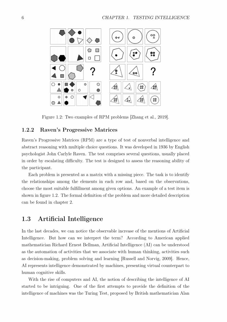
Figure 1.2: Two examples of RPM problems [Zhang et al., 2019].

1.2.2 Raven’s Progressive Matrices

Raven’s Progressive Matrices (RPM) are a type of test of nonverbal intelligence andabstract reasoning with multiple choice questions. It was developed in 1936 by Englishpsychologist John Carlyle Raven. The test comprises several questions, usually placedin order by escalating difficulty. The test is designed to assess the reasoning ability ofthe participant.

Each problem is presented as a matrix with a missing piece. The task is to identifythe relationships among the elements in each row and, based on the observations,choose the most suitable fulfillment among given options. An example of a test item isshown in figure 1.2. The formal definition of the problem and more detailed descriptioncan be found in chapter 2.

1.3 Artificial Intelligence

In the last decades, we can notice the observable increase of the mentions of ArtificialIntelligence. But how can we interpret the term? According to American appliedmathematician Richard Ernest Bellman, Artificial Intelligence (AI) can be understoodas the automation of activities that we associate with human thinking, activities suchas decision-making, problem solving and learning [Russell and Norvig, 2009]. Hence,AI represents intelligence demonstrated by machines, presenting virtual counterpart tohuman cognitive skills.

With the rise of computers and AI, the notion of describing the intelligence of AIstarted to be intriguing. One of the first attempts to provide the definition of theintelligence of machines was the Turing Test, proposed by British mathematician Alan

1.3. ARTIFICIAL INTELLIGENCE 7

Mathison Turing in 1950 in his paper Computing Machinery and Intelligence. Theobjective of the test is to exhibit intelligent behavior, indistinguishable from that of ahuman. The principle of the test resides in the communication between a program anda human interrogator via online typed messages. The interrogator’s task is to deter-mine, whether the responses come from a computer generating human-like responsesor a real person. The program successfully passes the test if the interrogator guessesincorrectly 30% of the time. Nowadays, computer programs still have problems withfooling sophisticated judges. However, many people have been misled when they hadno idea they might be in a conversation with a computer.

In recent years, a trend to create virtual personal assistants has emerged. Thesehumanlike companions are able to perform a wide variety of tasks. Evidently, thedevelopment of Artificial Intelligence is on the rise, with wide possible applications,ranging from the prediction of the customers’ behavior to humanoid robots.

Many tasks that AI could carry out do not require intelligence (as the ability tosolve abstract reasoning problems), similarly to human behavior. Despite this fact,we consider it an interesting subject for research to study this ability of computers.First of all, we need to select the right model for testing as a representative to simulatehuman cognition.

1.3.1 Artificial Neural Networks

One of the possible options, that could resemble humanlike reasoning, is to use Arti-ficial Neural Networks (ANNs). ANN is an abstracted model of the brain’s activity,simulating brain cells called neurons. A neural network is just a collection of unitsconnected together; the properties of the network are determined by its topology andthe properties of the “neurons” [Russell and Norvig, 2009].

The network consists of units, i.e. nodes, which are connected by directed links andorganized into layers. The links between nodes propagate activations a, simulatingthe performance of the biological brain cells. Every link between nodes i and j hasassigned a numeric weight wij, representing the strength of the connection, havingeither excitatory or inhibitory effect. Every neuron in the network produces outputbased on its input values and its activation function. To obtain the output of the unit,we need to compute a weighted sum of unit’s inputs as

netj =n∑

i=0

wijai (1.2)

where ai denotes the activation from unit i connected to j and n is the number ofconnected neurons from the previous layer or, in the case of input layer, the inputdimension. Then we apply the activation function as follows


aj = g(inputj) = g(n∑

i=0

wijai) (1.3)

where g is the neuron activation function. Some of the typically used functions arehyperbolic tangent, logistic sigmoid or softmax.

Once we have defined the units, we need to put them together and form a network.Then we propagate the signal from the input through the layers to the output. NNscan be built in various ways, basically forming either a feed-forward or a recurrentnetwork. The former type has connections between nodes in only one direction, soeach node collects input from the units of the preceding layer. The latter also takesin the outputs, making them additional inputs, hence creating a dynamic system.The response of the network depends also on the initial state, possibly depending onprevious inputs of the network. Hence, recurrent networks support short-term memory[Russell and Norvig, 2009], which can be advantageous in solving certain tasks.

Neural networks can be trained in several ways. Supervised learning is a method,when we train the network on input-target pairs (x1, y1), (x2, y2), ..., (xn, yn). Every yiwas generated by a function f(x) = y, which is unknown to the network. This way,we provide the network with a feedback, giving it the correct answers for the exampleinputs. The task is to find a function that sufficiently approximates f . Anotherapproach is referred to as unsupervised learning, where the network learns patterns inthe input without any explicit feedback (e.g. clustering).

Training the network involves a few stages. Firstly, we need to train the networkon the training set, which is usually the largest part of the dataset. It consists of theexample inputs, which are presented to the network so it can learn the features ofthe problem. The next step is to evaluate the model on the validation set to tune itsparameters. The validation set serves as an instrument to estimate the performanceof the network. Finally, once we have trained the best model on the training set, wetest it on the test set to measure the accuracy of its performance. The test set is a setof questions of the same problem type, but yet not seen by the network. This way wetest the generalization ability of the network, checking whether it is capable of dealingwith new instances of the problem and not just the ones it has already seen (which isachieved by their memorization).

1.4 Related Work

The first attempts of solving RPM led to the design of many AI agents and algorithms,which were based on the observation of the relationships shared between the cells inthe rows of the matrix [Joyner et al., 2015]. These approaches make use of additionalknowledge about the problem structure.

1.4. RELATED WORK 9

However, the idea of solving Raven’s Progressive Matrices with neural networkshas emerged in recent years. Neural networks do not need any additional information,performing automatic feature extraction without human intervention.

1.4.1 RAVEN Dataset

Solving RPM is not a simple task, not even for a human individual. Complex problemsdemand the use of deeper networks, which can extract the higher-level features from theinput. However, deep models require large datasets, otherwise they are prone to over-fitting the training data. This phenomenon is very undesirable, because it mitigatesthe generalization ability. Therefore, to be able to train the network properly, we needa sufficiently extensive dataset.

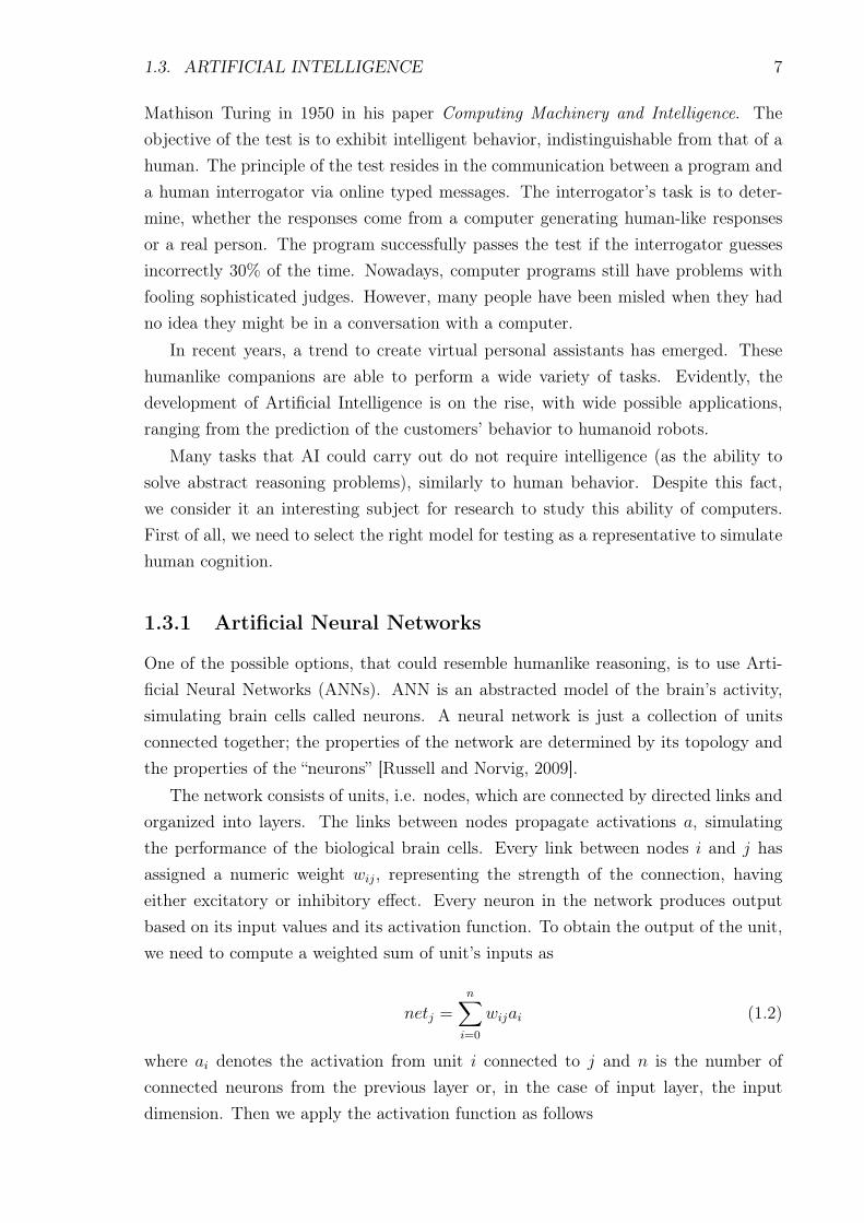
We decided to use RAVEN: A Dataset for Relational and Analogical Visual rEa-soNing, which was built in the context of Raven’s Progressive Matrices and aimed atlifting machine intelligence by associating vision with structural, relational, and ana-logical reasoning in a hierarchical representation [Zhang et al., 2019]. The dataset isalso provided with human performance as a reference. The dataset consists of 7 sub-types, which are depicted in figure 1.3. Each subtype contains 10 000 distinct problemscomprising 16 gray-scale images, as can be seen in figure 1.2.

The RPM matrices are generated based on a set of applicable rules. After thesampling of the rules for the matrix, they are used to create valid rows. The problemmatrix is then obtained as the concatenation of three distinct rows sharing the samerules. The answer set is generated by modifying the attributes of the correct choice ina way that breaks the rules of the matrix in the last row.

The rules are selected for every attribute individually and are chosen from 4 types:Constant, Progression, Arithmetic and Distribute Three. As can be derived from thename of Constant, this rule ensures that all the three images in the row share the samevalue of a certain attribute. Progression represents a quantitative increase or decreasebetween adjacent elements in the row and Arithmetic constrains the rows in a way thatthe attribute of the third item in the row is obtained by addition or subtraction of theattributes of the first two items. Distribute Three indicates three different attributevalues distributed through the row.

The human performance was evaluated by testing human subjects consisting ofcollege students on a subset of samples from the dataset types. First of all, they werepresented with a simple matrix with only one non-Constant rule to become familiarwith the problem. Then, they were tested on complicated questions with complex rulecombinations. The results, also with the comparison of various models they experi-mented with, can be found in table 1.1.


Figure 1.3: Different subtypes of RAVEN dataset [Zhang et al., 2019].

1.4.2 Solving RAVEN with Neural Networks

There have been proposed various perspectives and approaches for solving RPM withartificial neural networks so far.

The first attempts to experiment with the RAVEN dataset were performed right byits creators [Zhang et al., 2019]. They decided to try several well-known models to testtheir performance on the dataset. Considering the image representation of the problem,the authors decided to use models suitable for the task. In this case, as reasonablecandidates were chosen computer vision models, specifically Long Short-Term Memory(LSTM), Convolutional Neural Network (CNN), Residual Neural Network (ResNet)and Wild Relation Network (WReN).

LSTM is a type of a recurrent neural network, designed to process sequential datawith long-term dependencies. It is applicable to making the prediction of the nextelement in a series based on the dependencies in the input sequence. This seems tobe convenient for the RPM problem, as it is of a partially sequential character. Theauthors decided to extract the image features by a CNN, then pass them into theLSTM sequentially and predict the final answer by feeding the last hidden feature intoa multi-layer perceptron (MLP) with one hidden layer. Even though it may seem thatthis model suits the nature of the RPM problem, the results show that it was far fromthe best choice, yielding the average performance of only 13.07%.

In the second scenario, they set up a four-layer CNN followed by a two-layer MLP.The CNN extracts the image characteristics and the MLP applies the softmax activa-tion function to the output layer to classify the answer. The convolutional layers ofthe CNN are alternating with batch normalization and ReLU 1 layers. The last hiddenlayer of the MLP uses dropout regularization to reduce over-fitting. This structureended up more successful than the LSTM, the average result across the dataset typeswas 36.97%.

As the next model, they decided to try WReN, proposed specifically to solve RPM-like matrices [Barrett et al., 2018]. This model also uses a CNN for image featureextraction, but the features are then passed to a Relation Network module that formsrepresentations between each context component and each candidate answer, and be-tween the pairs of the context components themselves. It outputs scores for the can-

1activation function defined as f(x) = max(0, x)

1.4. RELATED WORK 11

Model Avg Center 2x2Grid 3x3Grid L-R U-D O-IC O-IG

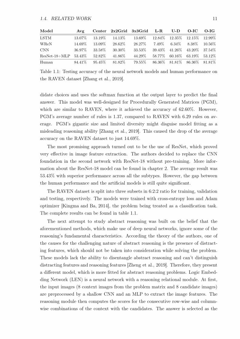
LSTM 13.07% 13.19% 14.13% 13.69% 12.84% 12.35% 12.15% 12.99%WReN 14.69% 13.09% 28.62% 28.27% 7.49% 6.34% 8.38% 10.56%CNN 36.97% 33.58% 30.30% 33.53% 39.43% 41.26% 43.20% 37.54%ResNet-18+MLP 53.43% 52.82% 41.86% 44.29% 58.77% 60.16% 63.19% 53.12%Human 84.41% 95.45% 81.82% 79.55% 86.36% 81.81% 86.36% 81.81%

Table 1.1: Testing accuracy of the neural network models and human performance onthe RAVEN dataset [Zhang et al., 2019].

didate choices and uses the softmax function at the output layer to predict the finalanswer. This model was well-designed for Procedurally Generated Matrices (PGM),which are similar to RAVEN, where it achieved the accuracy of 62.60%. However,PGM’s average number of rules is 1.37, compared to RAVEN with 6.29 rules on av-erage. PGM’s gigantic size and limited diversity might disguise model fitting as amisleading reasoning ability [Zhang et al., 2019]. This caused the drop of the averageaccuracy on the RAVEN dataset to just 14.69%.

The most promising approach turned out to be the use of ResNet, which provedvery effective in image feature extraction. The authors decided to replace the CNNfoundation in the second network with ResNet-18 without pre-training. More infor-mation about the ResNet-18 model can be found in chapter 2. The average result was53.43% with superior performance across all the subtypes. However, the gap betweenthe human performance and the artificial models is still quite significant.

The RAVEN dataset is split into three subsets in 6:2:2 ratio for training, validationand testing, respectively. The models were trained with cross-entropy loss and Adamoptimizer [Kingma and Ba, 2014], the problem being treated as a classification task.The complete results can be found in table 1.1.

The next attempt to study abstract reasoning was built on the belief that theaforementioned methods, which make use of deep neural networks, ignore some of thereasoning’s fundamental characteristics. According the theory of the authors, one ofthe causes for the challenging nature of abstract reasoning is the presence of distract-ing features, which should not be taken into consideration while solving the problem.These models lack the ability to disentangle abstract reasoning and can’t distinguishdistracting features and reasoning features [Zheng et al., 2019]. Therefore, they presenta different model, which is more fitted for abstract reasoning problems. Logic Embed-ding Network (LEN) is a neural network with a reasoning relational module. At first,the input images (8 context images from the problem matrix and 8 candidate images)are preprocessed by a shallow CNN and an MLP to extract the image features. Thereasoning module then computes the scores for the consecutive row-wise and column-wise combinations of the context with the candidates. The answer is selected as the



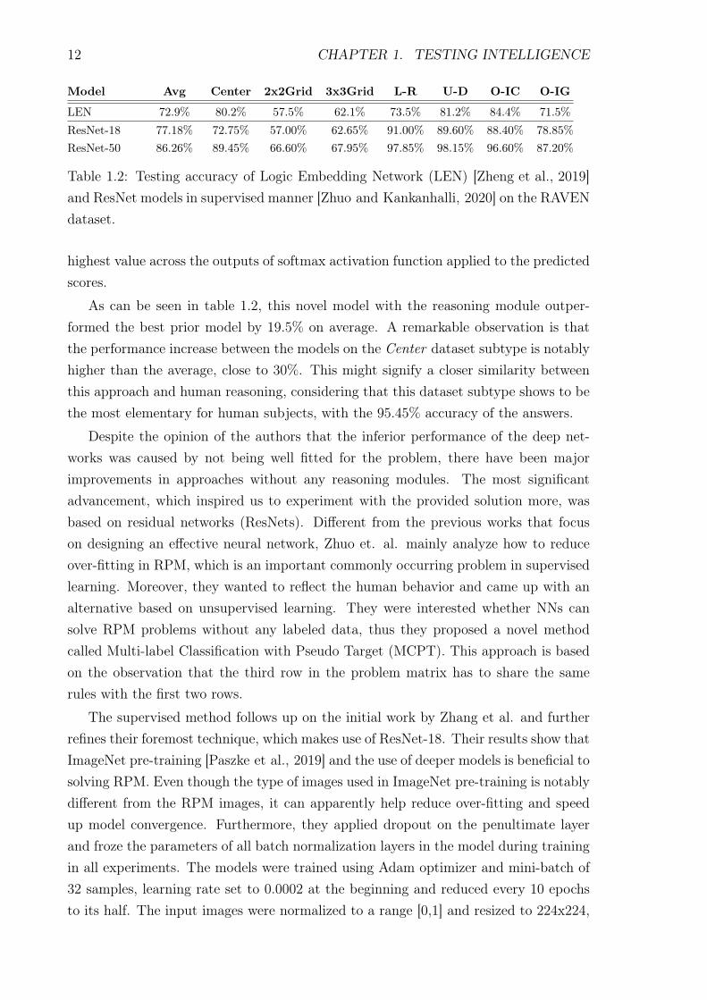
LEN 72.9% 80.2% 57.5% 62.1% 73.5% 81.2% 84.4% 71.5%ResNet-18 77.18% 72.75% 57.00% 62.65% 91.00% 89.60% 88.40% 78.85%ResNet-50 86.26% 89.45% 66.60% 67.95% 97.85% 98.15% 96.60% 87.20%

Table 1.2: Testing accuracy of Logic Embedding Network (LEN) [Zheng et al., 2019]and ResNet models in supervised manner [Zhuo and Kankanhalli, 2020] on the RAVENdataset.

highest value across the outputs of softmax activation function applied to the predictedscores.

As can be seen in table 1.2, this novel model with the reasoning module outper-formed the best prior model by 19.5% on average. A remarkable observation is thatthe performance increase between the models on the Center dataset subtype is notablyhigher than the average, close to 30%. This might signify a closer similarity betweenthis approach and human reasoning, considering that this dataset subtype shows to bethe most elementary for human subjects, with the 95.45% accuracy of the answers.

Despite the opinion of the authors that the inferior performance of the deep net-works was caused by not being well fitted for the problem, there have been majorimprovements in approaches without any reasoning modules. The most significantadvancement, which inspired us to experiment with the provided solution more, wasbased on residual networks (ResNets). Different from the previous works that focuson designing an effective neural network, Zhuo et. al. mainly analyze how to reduceover-fitting in RPM, which is an important commonly occurring problem in supervisedlearning. Moreover, they wanted to reflect the human behavior and came up with analternative based on unsupervised learning. They were interested whether NNs cansolve RPM problems without any labeled data, thus they proposed a novel methodcalled Multi-label Classification with Pseudo Target (MCPT). This approach is basedon the observation that the third row in the problem matrix has to share the samerules with the first two rows.

The supervised method follows up on the initial work by Zhang et al. and furtherrefines their foremost technique, which makes use of ResNet-18. Their results show thatImageNet pre-training [Paszke et al., 2019] and the use of deeper models is beneficial tosolving RPM. Even though the type of images used in ImageNet pre-training is notablydifferent from the RPM images, it can apparently help reduce over-fitting and speedup model convergence. Furthermore, they applied dropout on the penultimate layerand froze the parameters of all batch normalization layers in the model during trainingin all experiments. The models were trained using Adam optimizer and mini-batch of32 samples, learning rate set to 0.0002 at the beginning and reduced every 10 epochsto its half. The input images were normalized to a range [0,1] and resized to 224x224,

1.4. RELATED WORK 13


Random 12.50% 12.50% 12.50% 12.50% 12.50% 12.50% 12.50% 12.50%W/o MCPT 5.18% 7.60% 7.00% 7.00% 2.45% 3.20% 3.20% 5.30%W/ MCPT 28.50% 35.90% 25.95% 27.15% 29.30% 27.40% 33.10% 20.70%

Table 1.3: Testing accuracy of ResNet-18 in unsupervised manner[Zhuo and Kankanhalli, 2020] on the RAVEN dataset.

as the standard input shape of ResNet.Table 1.2 shows the results of the supervised experiments performed on the RAVEN

dataset. The model with ResNet-50 backbone outperforms LEN by 13.36% on average,which seems to refute the theory that ResNet-based models do not exhibit the abilityto distinguish between distracting and reasoning features. ResNet-50 surpasses theresults of LEN on every problem configuration and even ResNet-18 performs betterthan LEN on every configuration except for Center and 2x2Grid. But despite that,both of the ResNet models achieve the best results on the Left-Right and Up-Downsubsets, whereas for human subjects was Center the least problematic. Furthermore,the 2x2Grid and Out-InGrid are comparably complicated for humans, but the latterappears to be much more straightforward for the network. These differences mightindicate that the reasoning ability on the human level works in a slightly different way.

The unsupervised technique, called Multi-label Classification with Pseudo Target,is based on the fact that the three rows of the problem matrix have to satisfy thesame rules. The authors were inspired to explore the unsupervised solving techniquesby the human approach, dealing with RPM without any supervision or labeled data.They decided to use the ResNet-18 model with ImageNet pre-training and the sameimplementation setup as in the supervised experiments. For the demonstration of theeffectiveness of the method, they also provided the results of the model without apseudo target and the accuracy of random guess. As the results show, unsupervisedapproach without MCPT seems to be counterproductive, with the average accuracyeven below random guess. Given 8 candidate choices, the probability to select the rightanswer is 12.50%, which is 7.32% higher than the average correctness of the approachwithout MCPT. However, the approach with MCPT seems to be promising, morethan doubling the accuracy of random guess. Another interesting observation is thatthe model trained with the MCPT approach performs the best on the Center subset,similarly to human reasoning.

The unsupervised learning is a fascinating area, because it does not require labelsfor training which makes it usable in vast areas where labelled data are not available, oronly in small numbers. More detailed explanation of the MCPT approach is obtainablein chapter 2.


Chapter 2

Methodology and Implementation

In this chapter we state the aims and objectives of our work. The chapter also explainsthe methods used in the thesis and describes the implementation in detail.

2.1 Aims and Objectives

This thesis concerns the question, whether machines are capable of abstract reasoning,comparably to humans. In order to address this inquiry, we set the goals and specifythe steps that need to be taken to achieve the desired outcome.

Our aim is to investigate the ability of neural networks to solve Raven’s ProgressiveMatrices, a non-verbal IQ test widely used for testing human intelligence. We wouldalso like to further analyze the reasoning ability of the chosen model by the visualizationof its hidden representations. To achieve this, we implement a chosen neural networkand train it for solving RPM. We test the model’s generalization ability given varioussizes of the training set and the types of problems it consists of.

We decided to follow up on the work [Zhuo and Kankanhalli, 2020] and use ResNet-18 as the studied model. Their results show superior performance of the models basedon residual networks (see table 1.2). We use the publicly available implementation ofResNet-18 from the PyTorch library to make an unbiased comparison to the previouswork. We implement the training according to the information provided in the article[Zhuo and Kankanhalli, 2020] and perform the experiments on the RAVEN dataset[Zhang et al., 2019].

2.2 Problem Definition

Let X be a problem matrix with k elements and Y the answer set with l potential can-didates. To solve an RPM problem instance means to select the most fitting candidateyz to complete the matrix X, where z is the index of the candidate yz and z ∈ {1, ..., l}.

15

16 CHAPTER 2. METHODOLOGY AND IMPLEMENTATION

In the supervised approach, we are trying to learn a projection function f over(X, Y ) and Z, given we have n training samples {(xi, yi, zi) | 1 ≤ i ≤ n;xi ∈ X, yi ∈Y, zi ∈ Z}. The method can be formulated as

Z = f(φ(X ∪ Y ), w) (2.1)

where ∪ symbolizes the concatenation that stacks the images of the problem matrixwith the answer set images, φ denotes the image features over (X ∪ Y ) and w isthe hyperparameter the network is supposed to learn. This way, the RPM problemis considered as a multi-class classification task. The network is trained using cross-entropy loss, which is calculated for every problem as

loss(out, z) = − log(exp(outz)∑j exp(outj)

) (2.2)

where z is the target, i.e. the index of the correct answer, and out the output of thenetwork. As the final answer is selected the choice with the highest output probability.In the RAVEN dataset, we deal with matrices consisting of 8 images and the task isto select the 9-th element from 8 candidate choices to complete the matrix.

The aim of unsupervised approach is to find the correct answers for (X, Y ) with-out giving the network the answers to the problem instances during the training.The rows of the correctly completed matrix, i.e. (xi,1, xi,2, xi,3), (xi,4, xi,5, xi,6) and(xi,7, xi,8, yi,j); j ∈ {1, ..., 8}, have to share the same rules.

2.3 ResNet-18

ResNet-18 is a deep residual network having 17 convolutional layers and a fully-connected layer. Residual networks use skip connections, which makes them capable ofjumping over some layers. The addition of the skip connections helps the model withthe vanishing gradient problem and over-fitting, in case we use more than the suitablenumber of layers. The authors provide comprehensive empirical evidence showing thatthese residual networks are easier to optimize, and can gain accuracy from considerablyincreased depth [He et al., 2016].

The PyTorch implementation of the standard ResNet-18 model can be seen in figure2.1.

2.4 Supervised Learning

In this implementation, the images in the problem matrix X and in the correspondinganswer set Y are stacked together as the input for the neural network. Therefore,

2.4. SUPERVISED LEARNING 17

Figure 2.1: PyTorch implementation of standard ResNet-18.


we need to replace the first convolutional layer of the ResNet-18 model to expect 16-dimensional input. The output dimension of the fully-connected layer is set to 8, tocoincide with the number of potential candidates.

2.5 Multi-label Classification with Pseudo Target

The MCPT approach uses a pseudo target in a form of two-hot vector, which does notcontain the information about the correct answer. However, formally, it converts unsu-pervised learning to supervised. The vector is designed based on the observation thatthe rows are generated by applying the same rules. Therefore, the authors construct10 rows as can be seen in figure 2.2. The first two are taken directly from the problemmatrix and the rest 8 are produced as (xi,7, xi,8, yi,j); for all j ∈ {1, ..., 8}. The first 2values of the target vector are set to 1 and the other 8 to 0. This way, we force theoutputs for the rows with the candidate choices to get close to zero. The expectation isthat the row with the correct answer should keep producing higher output value thanthe rows with the incorrect ones, which should reflect the similarities of the correctlycompleted row and the two original rows from the matrix.

This unsupervised method can be represented by the formula

Z̃ = g(φ(X ∨ Y ), w) (2.3)

where Z̃ represents the pseudo target, which is the same for every RPM instance, φdenotes the image features, g is the projection function, (X ∨ Y ) are the rows, i.e.r1 = (xi,1, xi,2, xi,3), r2 = (xi,4, xi,5, xi,6), rj = (xi,7, xi,8, yi,j−2); for all j ∈ {3, ..., 10}.The rows constructed this way are then passed to the network to acquire their scores.The input layer of the standard ResNet-18 model is 3-dimensional, which is suitable forour input, although it is originally meant to take in RGB images. The images in theRAVEN dataset are grayscale, therefore they have only 1 color dimension, which meansthat we can fit in the whole row as the input in one step. The complete scores for eachRPM problem are obtained in 10 consecutive steps. The output layer is replaced bya fully-connected layer with one neuron that predicts the score of the input row. Thescores are then concatenated together and normalized by applying a sigmoid functionto get scores in range [0,1]. The model is trained using Binary Cross Entropy as theloss function, which can be described as

loss(out, z̃) = −n∑

i=1

[z̃i log outi + (1− z̃i) log(1− outi)] (2.4)

where z̃ is the pseudo target vector, z̃i ∈ {0, 1}, and out is the concatenated output ofthe network. During testing, the first two values of the prediction are removed and thecandidate filled in the row with the highest score is considered the final answer.

2.6. IMPLEMENTATION DETAILS 19

Figure 2.2: Schema of the MCPT approach [Zhuo and Kankanhalli, 2020].

2.6 Implementation Details

The differences in the model and training in the supervised and unsupervised approachare described in sections 2.4 and 2.5, respectively. This section presents the commonfeatures of the implementations.

From the wide variety of open source machine learning libraries, we decided to usePyTorch with the Python interface. ResNet-18 is one of the models that are imple-mented in the library, so we used the model pre-trained on the ImageNet dataset in allour experiments and made changes according to the article [Zhuo and Kankanhalli, 2020].We added a dropout with value 0.5 before the last layer to reduce over-fitting, which isa significant problem in deep networks. Moreover, we froze all the batch normalizationlayers in the model. For the training of the network, we used Adam optimizer withthe initial learning rate of 0.0002, which was reduced to its half every 10 epochs. Themodel was trained for 30 epochs, but it was validated after each epoch and as the finalstate for evaluation was selected the one with the highest validation accuracy. Then weperformed the testing on the testing parts of the dataset subsets. We used 6 folds fortraining, 2 for validation and 2 for testing. The input images were normalized to therange [0,1] and resized using bicubic interpolation to 224x224, which is the standardinput size for ResNet-18 in PyTorch. To speed up the training of the model, we ranthe computations on the GPU using CUDA technology developed by NVIDIA. TheCUDA Toolkit provides a comprehensive development environment for C and C++developers building GPU-accelerated applications [Cook, 2012], which was utilized bythe developers of PyTorch to accelerate the performance of the library.

We used UMAP for the visualization of the hidden representations on the penul-timate (average pooling) layer to look closer at the decisions of the network. UMAPis a general purpose manifold learning and nonlinear dimension reduction algorithm[McInnes et al., 2018], that is very popular for the visualizations in machine learning.

For more detailed description of the attached source codes see Appendix A.


Chapter 3

Experiments

This chapter describes the experiments that were performed on the RAVEN dataset,lists and interprets the obtained results.

3.1 Supervised Learning Experiments

3.1.1 Joint Training

First of all, we decided to replicate the basic experiment, which is demonstrated in[Zhuo and Kankanhalli, 2020]. The authors report their results on ResNet-18 withoutpre-training, but we use the model with ImageNet pre-training in our experiments.Otherwise, the experimental setup is identical to the one in their work. As table 3.1shows, the average accuracy of the models is very similar, which suggests that thepre-training does not play an important role in the final model generalization abilityin this case. The results of this experiment are used as the baseline for the comparisonof the latter experiments mentioned in the thesis.


w/o pre-train 77.18% 72.75% 57.00% 62.65% 91.00% 89.60% 88.40% 78.85%w/ pre-train (ours) 77.06% 78.30% 56.10% 59.65% 92.50% 91.15% 86.25% 75.50%

Table 3.1: Testing accuracy of supervised ResNet-18 without pre-training[Zhuo and Kankanhalli, 2020] on the RAVEN dataset compared to our experiment witha pre-trained model.

The results show that the pre-training causes the network to perform slightly betteron the subsets with less complicated image structure. The ImageNet dataset consistsof real-world images, which are very different from the ones in the RAVEN dataset.However, according to the article, the pre-training helps significantly with the trainingof the deeper ResNet models. Here it seems to help with the categories Center, where

21

22 CHAPTER 3. EXPERIMENTS

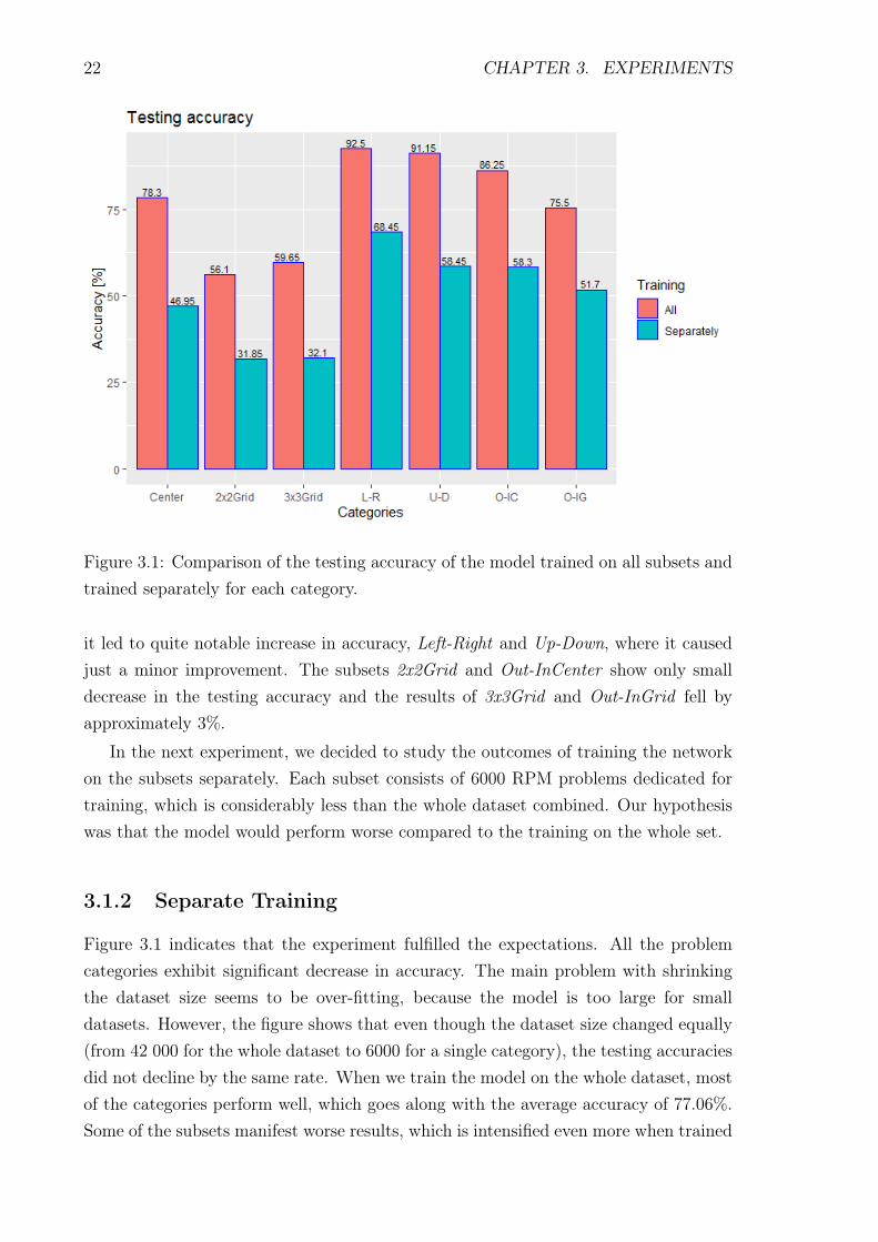
Figure 3.1: Comparison of the testing accuracy of the model trained on all subsets andtrained separately for each category.

it led to quite notable increase in accuracy, Left-Right and Up-Down, where it causedjust a minor improvement. The subsets 2x2Grid and Out-InCenter show only smalldecrease in the testing accuracy and the results of 3x3Grid and Out-InGrid fell byapproximately 3%.

In the next experiment, we decided to study the outcomes of training the networkon the subsets separately. Each subset consists of 6000 RPM problems dedicated fortraining, which is considerably less than the whole dataset combined. Our hypothesiswas that the model would perform worse compared to the training on the whole set.

3.1.2 Separate Training

Figure 3.1 indicates that the experiment fulfilled the expectations. All the problemcategories exhibit significant decrease in accuracy. The main problem with shrinkingthe dataset size seems to be over-fitting, because the model is too large for smalldatasets. However, the figure shows that even though the dataset size changed equally(from 42 000 for the whole dataset to 6000 for a single category), the testing accuraciesdid not decline by the same rate. When we train the model on the whole dataset, mostof the categories perform well, which goes along with the average accuracy of 77.06%.Some of the subsets manifest worse results, which is intensified even more when trained

3.1. SUPERVISED LEARNING EXPERIMENTS 23

separately.Left-Right is the most successful subset, with 92.50% accuracy, provided we train

the model on all the subsets combined together. Its accuracy drops to 68.45% whentrained separately. That represents decline by a quarter of the initial accuracy. A verysimilar result was obtained on Up-Down, where the training on the whole dataset endedwith the accuracy of 91.15%. The decrease was a bit stronger, resulting in 58.45%. Weconsider this very interesting, given the difference between Left-Right and Up-Downwas originally just 1.35% and one task is just a transposition of the other.

On the other hand, 2x2Grid performs much worse already in the first experiment.The accuracy starts on 56.10%, which is less than the accuracies of 3 of the othersubsets (Left-Right, Up-Down, Out-InCenter) trained separately. Moreover, if we train2x2Grid separately, the precision of the answers drops to 31.85%, which is the lowestof the results.

Another interesting point is that the ratio of the result obtained after the trainingon a single subset to the one after the training on the whole dataset varies with eachcategory. The smallest decrease is observable on the Left-Right subset, where the resultof the separate training presents 74.00% of the original result (decrease of 26.00%). Up-Down shows an absolute decrease of 32.70%, which is 35.87% relatively to the result ofthe training on the subsets combined. Also Out-InGrid and Out-InCenter demonstratecomparable fall of accuracy, of 31.52% and 32.41%, respectively. However, the resultsof the other categories diminished more significantly, Center by 40.04%, 2x2Grid by43.23% and 3x3Grid by 46.19% relatively to the prior results.

3.1.3 Combinations of 2 Categories

Since there are obvious differences between the subset performances, we decided tostudy the influence of the training on more subsets at once. We expected that it wouldhelp the model to improve its generalization ability.

To begin, we tried several combinations with the Center category. When trainedseparately, Center results in the accuracy of 46.95%. We tried the combinations with2x2Grid, Out-InGrid and Out-InCenter. As can be seen in figure 3.2, the correctnessof the answers on Center increased in every scenario, although by a bit different rate.The better the category scores separately, the more it helps to lift the accuracy ofCenter. However, the result of the other category in each experiment shows the oppositebehavior, so the better the category scores separately, the less its accuracy is raisedwhen trained together with Center. That means that the biggest increase is observableon 2x2Grid, where it increased by 8.9%, while the smallest is on Out-InCenter, wherethe accuracy rose from 58.3% to 63.8%, which makes the growth of 5.5%.

In the next experiment, we tried combinations with 2x2Grid. This is the subset


Figure 3.2: Results of the model trained on a combination of 2 subsets, where one ofthem is Center.

Figure 3.3: Results of the model trained on a combination of 2 subsets, where one ofthem is 2x2Grid.


that performs the worst when trained separately. When trained with Center (figure3.2), the accuracy rises to 40.75%. We tried to combine it with visually similar types- 3x3Grid and Out-InGrid. However, 2x2Grid did not perform better, compared totrained with Center, in any of these experiments. Also Out-InGrid does not demon-strate a greater increase in accuracy, showing the improvement of only 5.3%. Theresults are summarized in figure 3.3.

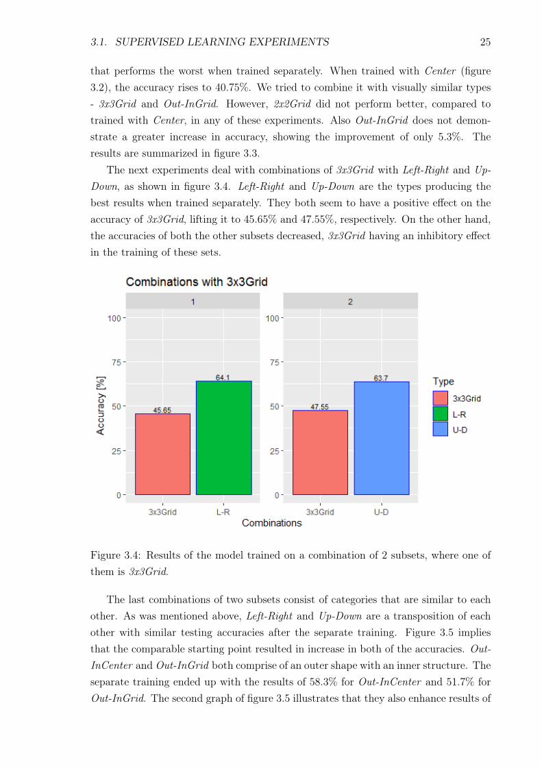
The next experiments deal with combinations of 3x3Grid with Left-Right and Up-Down, as shown in figure 3.4. Left-Right and Up-Down are the types producing thebest results when trained separately. They both seem to have a positive effect on theaccuracy of 3x3Grid, lifting it to 45.65% and 47.55%, respectively. On the other hand,the accuracies of both the other subsets decreased, 3x3Grid having an inhibitory effectin the training of these sets.

Figure 3.4: Results of the model trained on a combination of 2 subsets, where one ofthem is 3x3Grid.

The last combinations of two subsets consist of categories that are similar to eachother. As was mentioned above, Left-Right and Up-Down are a transposition of eachother with similar testing accuracies after the separate training. Figure 3.5 impliesthat the comparable starting point resulted in increase in both of the accuracies. Out-InCenter and Out-InGrid both comprise of an outer shape with an inner structure. Theseparate training ended up with the results of 58.3% for Out-InCenter and 51.7% forOut-InGrid. The second graph of figure 3.5 illustrates that they also enhance results of


each other when trained together and the joint training reduces the difference betweentheir accuracies.

Figure 3.5: Results of the model trained on a combination of 2 visually similar subsets.

3.1.4 Combinations of 3 Categories

The results of the previous experiments suggest that the size of the training set playsa significant role in the model generalization ability. However, the outcome obviouslydepends also on which of the categories are joined together. Therefore, we decided tolook into this further and perform experiments with triplets of categories.

First of all, we tried to combine three subsets that do not have much in commonand then compare it to a triplet consisting of somehow connected subsets. The firstgroup contains Center, 3x3Grid and Out-InGrid. Figure 3.6 illustrates the contrastbetween the separate training and the joint training of these three problem categories.

The second triplet consists of Center, 2x2Grid and Out-InGrid. These categorieshave a visually detectable connection. Out-InGrid comprises of an outer shape, whichis similar to Center, and an inner structure of 2x2Grid. Moreover, the results should becomparable, because 2x2Grid and 3x3Grid produce very similar results when trainedseparately. As figure 3.6 shows, there is a difference to some extent between the re-sults of the experiment with 2x2Grid, compared to the one with 3x3Grid (figure 3.6).3x3Grid manifests a bigger increase in accuracy than 2x2Grid, but 2x2Grid enhances


Figure 3.6: Results of the model trained on 3 subsets. Darker colors represent theaccuracy of the combined training and lighter the results obtained after separate train-ing.


the results of Center and Out-InGrid more.The next experiment deals with subsets Center, Left-Right and Up-Down. The

combination of Left-Right and Up-Down was very successful, therefore we were inter-ested, what effect might have the addition of another category into training. It is alittle complicated to decide which category has the most similar structure, so we choseCenter as it has the most elementary structure. Figure 3.6 displays surprising resultsof the experiment. Not only did not the addition of Center help to increase the testingaccuracy of Left-Right and Up-Down, it led to a significant decrease, compared to thejoint training of these 2 categories.

As the last experiment with a triplet, we chose the 3 subsets producing the bestresults when trained separately, which are Left-Right, Up-Down and Out-InCenter.We assumed that they have a potential to improve each other’s performance. Thisassumption was confirmed, supported by the results in figure 3.6. Each category ex-hibits a significant improvement, scoring over 80%. The average increase is 24.5%,which advances the accuracies almost to the level of the training of all the problemtypes together. In that scenario, Left-Right scores 92.5%, which is only 3.75% more,Up-Down 91.15%, which is a 4% difference and Out-InCenter 86.25%, which is 3.45%over the result of this combination.

3.1.5 Excluding Categories

After observing the differences between the separate training and the training of com-binations, there arose a question, how would excluding certain categories from thewhole training set affect the results. We decided to study 2 groups of types with visualconnections - Left-Right with Up-Down, and 2x2Grid with 3x3Grid and Out-InGrid.

In the first set of experiments, we began with excluding only Left-Right. As can beseen in figure 3.7, the result of every category decreased a little. The most significantdecline is observable on the Left-Right category, as expected. The average decreaseamong the trained categories is 2.38%, while the untrained subset got worse by 22.35%.

Then we excluded only Up-Down and compared the results. Figure 3.8 portays thecomparison to the training of the whole training set. The results are similar to thefirst experiment, the average decrease is 2.25%, provided we take into consideration thetrained subsets. The performance of Up-Down declined by 15.45%, which is notablyless than the decrease of untrained Left-Right.

Lastly, we exclude both of the subsets, training on the remaining 5 categories.From figure 3.9 is observable that both of the excluded categories perform even worsethan when excluded individually. Compared to the previous two experiments, all theproblem types produce worse results. The average decrease of the trained subsets is6.85% and among all the subsets 12.22%.


Figure 3.7: Results of the model trained on the whole training set, excluding Left-Right.

Figure 3.8: Results of the model trained on the whole training set, excluding Up-Down.

The second group was formed around the subset 2x2Grid, because it producesthe worst score. At first, we excluded only the one and observed the changes in the


Figure 3.9: Results of the model trained on the whole training set, excluding Left-Rightand Up-Down.

scores. Figure 3.10 shows the results of training without 2x2Grid. As expected, all thecategories display a decrease in accuracy. However, it is interesting that the excludeddataset did not drop very much, only by 10.6%, similarly to other categories.

When we exclude 2x2Grid and also 3x3Grid, all the categories, except for 3x3Grid,manifest a smaller decrease in testing accuracy, as shown in figure 3.11. When exclud-ing only 2x2Grid, the average decrease is 9.07%, when excluding both 2x2Grid and3x3Grid, the decrease changes to 7.08%. This is remarkable, given we reduce the sizeof the training set.

We further analyze the outcomes by excluding 2x2Grid andOut-InGrid. Figure 3.12implies a similar behavior as when we exclude 2x2Grid with 3x3Grid. This trainingset also results in a smaller decrease of accuracy of every problem type, except forOut-InGrid, compared to excluding only 2x2Grid. The average decrease dropped to7.35%, which is similar to case of excluding 2x2Grid and 3x3Grid.

The final experiment deals with the consequences of excluding the whole group(2x2Grid, 3x3Grid and Out-InGrid), the results are summarized in figure 3.13. Theexperiment copies the trend of the previous ones, resulting in an even smaller decreaseof 6.43%. All the included subsets show a better performance, compared to excludingless subsets, while the accuracy of the excluded ones slightly varies.


Figure 3.10: Results of the model trained on the whole training set, excluding 2x2Grid.

Figure 3.11: Results of the model trained on the whole training set, excluding 2x2Gridand 3x3Grid.


Figure 3.12: Results of the model trained on the whole training set, excluding 2x2Gridand Out-InGrid.

Figure 3.13: Results of the model trained on the whole training set, excluding 2x2Grid,3x3Grid and Out-InGrid.

3.2. UNSUPERVISED LEARNING EXPERIMENTS 33

3.2 Unsupervised Learning Experiments

The unsupervised approach from the article is based on an interesting principle, so wealso tried to perform a few experiments inspired by the MCPT approach. Firstly, wetried to replicate the experiment and compare the outcomes. As shown in table 3.2,the experiment ended up unsurprisingly, producing results very similar to the ones inthe article.


Zhuo et. al. 28.50% 35.90% 25.95% 27.15% 29.30% 27.40% 33.10% 20.70%Ours 27.79% 36.00% 23.95% 28.50% 27.20% 24.95% 32.15% 21.75%

Table 3.2: Testing accuracy of ResNet-18 in unsupervised manner[Zhuo and Kankanhalli, 2020] on the RAVEN dataset compared to our results.

Figure 3.14: Results of the model trained on the whole training set in an unsupervisedmanner in various scenarios.

The next experiments preserve the nature of the MCPT approach. The averageaccuracies are depicted in figure 3.14 and compared to the basic MCPT approach.The first two experiments are based on the modification of the pseudo target vector.The target in MCPT is a vector of 2 ones and 8 zeros. In our first experiment, wekeep the first 2 values and the 8 are chosen randomly from the uniform distributionin range [0,0.5]. The underlying hypothesis was that, rather than to force the outputs


to predict zero during training, the corresponding output neurons would be providedwith arbitrary information, statistically balanced. In this aapoach, there could still beincentive to build internal representations that could help the correct output canidate toproduce the highest output value drawing on shared similarities with the first two rowsof inputs. This experiment did not end up better than the original MCPT approach,with the testing accuracy of 24.8%. In the second experiment, one of the 8 zeros isreplaced with one, chosen randomly. This way, we do not tell the network the correctanswer, but we let it know that there exists one. However, this did not help to improvethe accuracy either, resulting in 24.06% accuracy. The last unsupervised experimentuses the original pseudo target, but the initial learning rate for the output layer isset to half the learning rate of other layers, being 0.0001. As the figure shows, themodification did not make a difference, compared to the MCPT. Unfortunately, wedid not come up with a technique that would improve the results in an unsupervisedmanner.

3.3 Visualization and Interpretation of the Results

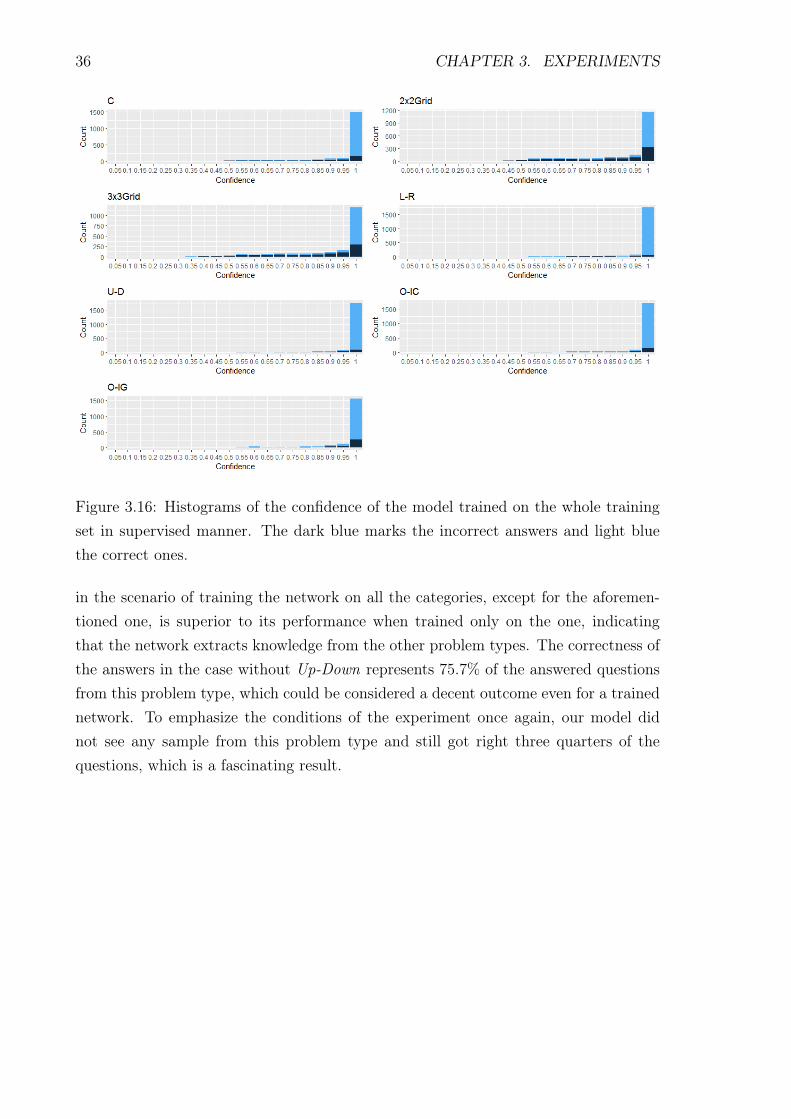
To further analyze the behavior of the network, we looked into it and collected the ac-tivations of the penultimate layer. To reduce the high dimensionality for visualization,we used UMAP and plotted it in 2D. Figure 3.15 displays the hidden representationsof the model trained on the whole RAVEN dataset. The answers seem to form clus-ters based on the winner neuron. We noticed that the clusters of Left-Right are muchmore separated than the clusters of the worse performing subsets, e.g. 2x2Grid. To ex-plain this phenomenon, we measured the confidence of the network while answering thequestions. This proved to be the answer, as captured in figure 3.16. The subsets withhigher accuracy demonstrate higher confidence, which results in more distant clustersof answers.

It is difficult to interpret the results, more accurate interpretation would need tostudy and somehow precisely measure the similarities of the problem categories. Webased the selections of the subsets in our experiments on their visual similarities. More-over, we decided to always train the model either on the whole subset or on none of itsitems, never training just a certain portion. It is known that reducing the number ofthe training samples decreases the accuracy of neural network models and we focusedon the dynamics of the model given various types of questions. However, some of theresults look very interesting, suggesting that the network profits from the knowledgeacquired from the other problem types.

Concerning the training on the combinations of 3 subsets, it is apparent that thesmallest improvement was notable on the combination of 3 random ones, i.e. those that

3.3. VISUALIZATION AND INTERPRETATION OF THE RESULTS 35

Figure 3.15: Visualization of the hidden representations on the penultimate layer ofthe model trained on the whole training set in a supervised manner. The differentcolors illustrate the order of the answer chosen by the network (1 to 8), i.e. the mostactivated output neuron.

are visually dissimilar. On the contrary, the highest advance showed the experimentwith the subsets with visually observable connection - Center, 2x2Grid and Out-InGrid.Although, we consider interesting that this combination resulted in significantly higheraccuracy of Center and not Out-InGrid as we expected (compared to the randomcombination of Center, 3x3Grid and Out-InGrid). This behavior remains unclear andwould need further research.

Another interesting observation is that when we excluded the 2x2Grid, the accuracyof the other subsets dropped more than when we excluded both 2x2Grid and 3x3Grid.The similar situation arose when we excluded 2x2Grid and Out-InGrid. Furthermore,excluding all three of these subsets seemed to be the best option, suggesting theseproblem types are perceived in a similar manner by the network.

The second studied group of excluded subsets also produces intriguing results.When we trained all the subsets with the exception of Left-Right, the decrease ofits accuracy was less significant than when we excluded both Left-Right and Up-Down.The same is notable when eliminating only Up-Down from the training, its accuracy ishigher than when omitting both of the subsets. We assume there is a certain connectionbetween these two problem types from the network’s point of view.

The last observation we would like to point out is that the performance of Up-Down


Figure 3.16: Histograms of the confidence of the model trained on the whole trainingset in supervised manner. The dark blue marks the incorrect answers and light bluethe correct ones.

in the scenario of training the network on all the categories, except for the aforemen-tioned one, is superior to its performance when trained only on the one, indicatingthat the network extracts knowledge from the other problem types. The correctness ofthe answers in the case without Up-Down represents 75.7% of the answered questionsfrom this problem type, which could be considered a decent outcome even for a trainednetwork. To emphasize the conditions of the experiment once again, our model didnot see any sample from this problem type and still got right three quarters of thequestions, which is a fascinating result.

Summary

Neural networks are often considered and used as "black boxes" by the unversed com-munity. We chose the opposite approach and looked inside into the network to try toexplain its decision-making process. We successfully tested the generalization abilityof the network, resulting in various interesting observations. Some of our experimentsask for further investigation to clarify the behavior of the network.

Most importantly, the chosen model is very effective in image feature extraction,which makes a strong foundation for it to cope with more difficult visual problems,such as solving RPM. We consider it remarkable that the unsupervised MCPT ap-proach achieves better results than certain well-known models or models dedicated tosolve RPM-like matrices trained in supervised manner (LSTM, WReN). Although wedid not succeed in improving the MCPT method, we realize the significance of unsu-pervised approaches and therefore encourage other researchers to attempt to refine thetechnique.

The experiments performed within the thesis point to the potential of neural net-works in the field of abstract reasoning. The training on the whole RAVEN datasetproduces superior results, suggesting that the networks profits from learning on severalproblem categories. However, the selection of the training subsets proved to be verysignificant as certain combinations produce better results than others, even though thesize of the training set is the same. The worse results obtained during the separatetraining might be caused by the significant reduction of the size of the training set,cutting it to 1/7. ResNet-18 is a deep model, requiring extensive datasets, and 6000training samples may not be sufficient to properly train the network. Nevertheless, Left-Right shows a decent performance, answering correctly 68.45% of the questions. Hence,Left-Right trained separately outperforms 2x2Grid and 3x3Grid trained together withthe rest of the problem categories. The combinations of 2 similar subsets (Left-Rightand Up-Down, Out-InCenter and Out-InGrid) also achieved good results, suggesting aconnection between the combined types. The most successful triplet turned out to bethe one consisting of the subsets with the highest accuracy demonstrated in the sep-arate training. Also excluding certain problem types from the training set producedinteresting results (e.g. excluding 2x2Grid, 3x3Grid and Out-InGrid produced betterresults than excluding only 2x2Grid), worthy of additional research.

37

38 Summary

To conclude, the average testing accuracy of the supervised approach does notreach the level of humans, but some of the categories achieve even better results. Tocontinue in our research, we propose to design a metrics to quantify the extent ofsimilarity among the problem types based on their features and not only on our visualperception. It could be also interesting to quantify the similarities among the optionsin the answer set and study the wrong answers of the network. We tried to do thisby visually checking the incorrectly answered questions and the corresponding answersets and noticed that the answers chosen by the network were very similar to thecorrect ones, likely fooling also human subjects. Hence, the results of the performedexperiments suggest that the tested model is showing signs of abstract reasoning.

Bibliography

[Barrett et al., 2018] Barrett, D., Hill, F., Santoro, A., Morcos, A., and Lillicrap, T.(2018). Measuring abstract reasoning in neural networks. In International Confer-ence on Machine Learning, pages 511–520. PMLR.

[Binet et al., 1916] Binet, A., Simon, T., and Kite, E. (1916). The development ofintelligence in children (The Binet-Simon Scale). Williams & Wilkins Co.

[Braaten and Norman, 2006] Braaten, E. B. and Norman, D. (2006). Intelligence (IQ)Testing. Pediatrics in Review, 27(11):403–408.

[Cook, 2012] Cook, S. (2012). CUDA Programming: A Developer’s Guide to ParallelComputing with GPUs. Morgan Kaufmann Publishers Inc., San Francisco, CA, USA,1st edition.

[Galton, 1891] Galton, F. (1891). Hereditary Genius. D. Appleton.

[He et al., 2016] He, K., Zhang, X., Ren, S., and Sun, J. (2016). Deep Residual Learn-ing for Image Recognition. In Proceedings of the IEEE Conference on ComputerVision and Pattern Recognition (CVPR).

[Hunt, 2010] Hunt, E. (2010). Human intelligence. Cambridge University Press.

[Joyner et al., 2015] Joyner, D. A., Bedwell, D., Graham, C., Lemmon, W., Martinez,O., and Goel, A. K. (2015). Using Human Computation to Acquire Novel Methodsfor Addressing Visual Analogy Problems on Intelligence Tests. In InternationalConference on Computational Creativity (ICCC), pages 23–30.

[Kingma and Ba, 2014] Kingma, D. P. and Ba, J. (2014). Adam: A method for stochas-tic optimization. arXiv–1412.

[McInnes et al., 2018] McInnes, L., Healy, J., and Melville, J. (2018). UMAP: Uniformmanifold approximation and projection for dimension reduction. arXiv–1802.

[Paszke et al., 2019] Paszke, A., Gross, S., Massa, F., Lerer, A., Bradbury, J., Chanan,G., Killeen, T., Lin, Z., Gimelshein, N., Antiga, L., Desmaison, A., Kopf, A., Yang,

39

40 BIBLIOGRAPHY

E., DeVito, Z., Raison, M., Tejani, A., Chilamkurthy, S., Steiner, B., Fang, L., Bai,J., and Chintala, S. (2019). Pytorch: An imperative style, high-performance deeplearning library. In Advances in Neural Information Processing Systems 32, pages8024–8035. Curran Associates, Inc.

[Raven and Court, 1938] Raven, J. C. and Court, J. (1938). Raven’s progressive ma-trices. Western Psychological Services Los Angeles, CA.

[Russell and Norvig, 2009] Russell, S. and Norvig, P. (2009). Artificial Intelligence: AModern Approach. Prentice Hall Press, USA, 3rd edition.

[Sternberg, 2000] Sternberg, R. J. (2000). Handbook of intelligence. Cambridge Uni-versity Press.

[Zhang et al., 2019] Zhang, C., Gao, F., Jia, B., Zhu, Y., and Zhu, S.-C. (2019). Raven:A dataset for relational and analogical visual reasoning. In Proceedings of the IEEEConference on Computer Vision and Pattern Recognition (CVPR).

[Zheng et al., 2019] Zheng, K., Zha, Z.-J., and Wei, W. (2019). Abstract reasoningwith distracting features. arXiv:1912.00569.

[Zhuo and Kankanhalli, 2020] Zhuo, T. and Kankanhalli, M. (2020). Solving raven’sprogressive matrices with neural networks. arXiv–2002.

Appendix A

Contents of the Electronic Attachment

The electronic attachment contains the source codes used for the experiments and theresults. The file network.py defines the model, util.py defines the training functionsand main.py loads the data and runs the program. The files are divided into supervisedand unsupervised part, the source codes for the models slightly differ.

41

Documents

Testing neural network intelligence using Raven’s