Testing McBratney et al.’s (2005) Model About …€¦ · (% sand, silt, clay) Laser methods/finger-texturing Volumetric water content (VWC) (%) Delta-T theta probe (5 replicates

Geography Department

Testing McBratney et al.’s (2005) Model About Relations Between Electrical Conductivity Data and Soil Properties: Is it of Practical

Use In Soil Survey?Ruth Kerry and Elizabeth B. Gillins

Department of Geography, Brigham Young University


Introduction

• Using electrical conductivity data (ECa) in soil survey and particularly for Precision Farming has become popular because it is related to several soil properties that could affect crop yield

• Theoretically sound reasons exist to explain these relationships but they vary spatially making interpretation of ECa patterns difficult even within fields

• Some have advocated using ECa data to show relationships with soil properties for which there is no theoretical basis


Introduction

• Most ECa research has involved establishing relationships with soil properties or uses ECa as a covariate for co-kriging or regression kriging -this may not be the best use of it (McBratney et al., 2005).

• Theoretically sound relationships developed between high frequency devices like time-domain reflectometers can be used to inform interpretation of the lower frequency ECa data (McBratney et al., 2005).


McBratney et al.’s (2005) Model

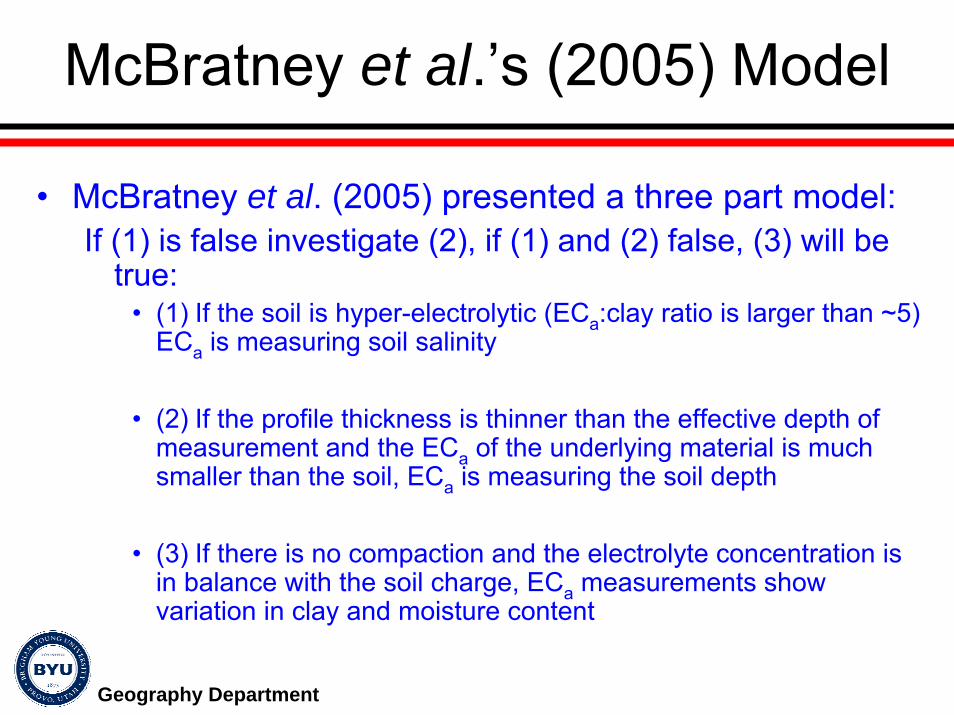
• McBratney et al. (2005) presented a three part model:If (1) is false investigate (2), if (1) and (2) false, (3) will be

true:• (1) If the soil is hyper-electrolytic (ECa:clay ratio is larger than ~5)

ECa is measuring soil salinity

• (2) If the profile thickness is thinner than the effective depth of measurement and the ECa of the underlying material is much smaller than the soil, ECa is measuring the soil depth

• (3) If there is no compaction and the electrolyte concentration is in balance with the soil charge, ECa measurements show variation in clay and moisture content


Research Purpose

Test the validity of McBratney et al.’s (2005) model at several field sites on

different parent materials that are likely to satisfy the conditions of the

model and determine if it is of practical use to soil survey


Site Description

• Soil samples were obtained at five arable field sites in southern England and one in Utah

• The soil parent materials at the sites were: – Shuttleworth: Lower Greensand – 11.77 ha – Wallingford: flint and quartzite pebble gravel – 43.54 ha – Yattendon: Chalk – three fields Y214 – 10.35 ha, Y215

– 15.27 ha and Y217 – 35.17 ha– Utah (work in progress)


Soil Sampling Schemes

• Top-soil (0-15 cm) sampled on 20-m (Shuttleworth) and 30-m grids (Wallingford and Yattendon)

• 6 cores from 1 m2 were bulked

Wallingford Yattendon – Y214


Field and Lab Methods

Salinity not measured at England sites

Soil property Method

Compaction

Soil structure observations (Hodgson, 1974)

Depth (cm)

Auger and tape measure

Salinity

ECa of soil extract (Rowell, 1994)

Stoniness (%)

Standard charts (Hodgson, 1976)

Texture (% sand, silt, clay)

Laser methods/finger-texturing

Volumetric water content (VWC) (%)

Delta-T theta probe (5 replicates within 1 m2) calibrated for soil type


ECa Collection

• Geonics EM38 in the vertical position used

• ECa is measured to a depth of about 1.5m, but the main signal is received from the top 30-50 cm of soil

• ECa is affected by moisture so data was collected when the soil was at about field capacity

DGPS Receiver

Data logger

EM38


ECa Collection

180000

180200

180400

180600

180800

455600 455800 456000 456200 456400 456600 456800 457000 457200 457400

Easting (m)

Nor

thin

g (m

)191800

192000

192200

192400

192600

192800

193000

464400 464600 464800 465000 465200 465400 465600 465800

Easting (m)

Nor

thin

g (m

)

244700

244800

244900

245000

245100

245200

245300

514050 514150 514250 514350 514450

Easting (m)

Nor

thin

g (m

)

• ECa values collected on transects about 20 m apart

• position and measurement recorded every 2 seconds Y214 Y215

Wallingford

Y217

Shuttleworth


Resistivity Collection• The resistivity of the soil (its resistance per unit length) was

measured in Ω.m using a GEOPULSE resistivity meter under computer control with 20 electrodes spaced 1 m apart

• Effective measurement depths = 25, 75, 127, 185, 250 and 320 cm• Resistivity data shows how the ECa changes with depth

A a a a a a a a a a a a a a a a a a a

25cm75 cm127cm185 cm250 cm320 cm

Laptop computer

Depth

5651

43

118

32Electrode

Station

Resistivity meter

Apparent resistivity (R) is the reciprocal of ECa (K)

R = 1/K


Data Analysis

• Average of all points within 20 or 30m of a soil sampling grid node (Kerry and Oliver, 2003) calculated to get ECa values for correlation with soil properties

• Moving correlations were calculated between soil properties and ECa at each soil sampling point using a (5 x 5) moving window

• Correlations > 0.381 are significant at the 0.05 level, and correlations > 0.45 moderate


Data Analysis• Indicator (binary, 0 or 1) variables were made from

correlations between ECa and the soil properties

• Correlation coefficients > 0.45, indicator = 1, else = 0

• Indicator variables made for each condition of McBratneyet al.’s (2005) model :– (1) ECa:clay ratio >5, indicator = 1, else = 0 – (2) Soil depth < 30 or 50cm, indicator = 1, else = 0– (3) Soil compacted, indicator = 1, else = 0

• Indicators variograms computed and maps produced by indicator kriging (Goovaerts, 1997).


RESULTS


Results: Summary all Sites

* Variable not measured at site

Proportion of sampling points meeting conditions 1-3 of McBratney et al.’s (2005) model

Site 1) Hyper-electrolytic 2) <30cm deep 2) <50cm deep 3) no compaction (%) (%) (%) (%) Shuttleworth 0 * * 94 Wallingford 0 9 51 75 Y214 0 52 87 67 Y215 0 70 98 68 Y217 0 18 31 47 Spanish Fork * * *

Utah


Results: Summary all Sites

* Variable not measured at site or no values with correlation greater than 0.45

P - proportion (%) of sampling points with moderate correlation >0.45 Rall - correlation coefficient for the whole dataset Rmax.- maximum correlation coefficient observed for a sampling point

Relationships between ECa and selected soil properties

Site Depth Clay VWC Sand Stones

P Rall Rmax P Rall Rmax P Rall Rmax P Rall Rmax P Rall Rmax

Shuttleworth * * * 38 0.38 0.77 19 0.46 0.72 51 -0.51 -0.85 25.20 0.23 0.74

Wallingford 3 0.36 0.61 39 0.57 0.86 38 0.59 0.91 44 -0.65 -0.89 27.03 -0.54 -0.92

Y214 50 0.47 0.72 9 0.06 -0.66 31 0.57 0.59 37 0.55 0.85 35.29 -0.52 -0.69

Y215 0 0.16 * 2 0.07 -0.51 20 0.53 0.55 3 0.18 0.56 22.03 -0.39 -0.66

Y217 20 0.38 0.65 30 -0.05 0.74 6 0.10 -0.49 0 0.05 * 41.38 -0.28 -0.83

Spanish Fork * * * Utah


Results: Wallingford (Condition 2)

• Resistivity decreases with depth• ECa increases with depth • Condition (2) of model is not met

Probability of > 0.45 correlation between ECa and depth

Probability of depth < 30 cm Probability of depth < 50 cm


Results: Wallingford (Condition 3)Probability of compaction

Probability of > 0.45 correlation between ECa and sand

Probability of > 0.45 correlation between ECa and clay

Probability of > 0.45 correlation between ECa and VWC


Results: WallingfordECa Clay Sand

Depth VWC Stones


Results: Yattendon 214 (Condition 2)

• Resistivity increases with depth• EC decreases with depth • Condition (2) of model is met

Probability of > 0.45 correlation between ECa and depthProbability of depth < 30 cm Probability of depth < 50 cm


Results: Yattendon 214 (Condition 3)

Probability of compactionProbability of > 0.45 correlation

between ECa and sandProbability of > 0.45 correlation

between ECa and clay

Probability of > 0.45

correlation between ECa

and VWC


Results: Yattendon Field 214ECa Clay Sand

Depth VWC Stones


Practical Method

Standard charts suggest ECa decreases with depth at both sites

HighHigh

Medium

MediumLow

Low

Conditions of McBratney et al.’s (2005) model Zone Hyper-electrolytic Depth < 30cm No compaction

Number of points Depth of points (cm)

Number of points

Number of points

Wallingford - High 0 26,36,37,56,72 1 5 Wallingford - Medium 0 67,70,73,79,82 0 1 Wallingford – Low 0 30,34,34,42,52 1 5 Yattendon – High 0 24,38,43,63,67 1 0 Yattendon - Medium 0 27,33,34,34,120 1 5 Yattendon - Low 0 23,23,32,33,42 2 5

Five points located in each

zone


Conclusions• Within most fields different conditions from the model apply in

different parts of the field

• In some fields or parts of fields, none of the conditions from the theory apply

• A depth of 30 cm is useful as an effective depth of measurement for the Geonics EM38 at Wallingford and Yattendon sites

• Perhaps soil stoniness should be included in the model

• Summary results helpful: the proportion of sampling points that met a condition was similar to the proportion of points where there was a > 0.45 correlation with ECa and Kriging of indicators was helpful to determine where these tended to coincide spatially


Conclusions

• McBratney et al.’s (2005) model can provide interpretative insight into what ECa data is measuring

• There are gaps in this model which need to be addressed:– What is ECa measuring when none of the three model conditions

applies? – How should one test if the electrolyte is in balance with the soil

charge? – Practical problems of using the model effectively - intensive soil

analysis for this study has shown that testing each model condition at many sampling points would be impractical defeating the object of the model which is to save time and money for soil survey by interpreting ECa data correctly


Conclusions

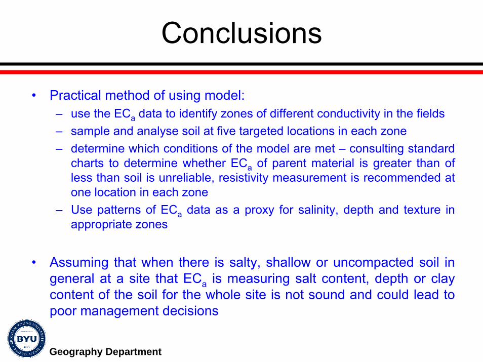
• Practical method of using model: – use the ECa data to identify zones of different conductivity in the fields– sample and analyse soil at five targeted locations in each zone – determine which conditions of the model are met – consulting standard

charts to determine whether ECa of parent material is greater than of less than soil is unreliable, resistivity measurement is recommended at one location in each zone

– Use patterns of ECa data as a proxy for salinity, depth and texture in appropriate zones

• Assuming that when there is salty, shallow or uncompacted soil in general at a site that ECa is measuring salt content, depth or clay content of the soil for the whole site is not sound and could lead to poor management decisions


Acknowledgements

We thank:– The Fertiliser Manufacturers’ Association and The

Research Endowment Trust Fund (RETF) of the University of Reading and the Office of Research and Creative Activities (ORCA) of Brigham Young University for funding this research

– SOYL Ltd. and Turftrax for collecting ECa data– Grant Cardon of Utah State University and Bruce

Webb of Brigham Young University for advise and use of equipment

Documents

Testing McBratney et al.’s (2005) Model About …€¦ · (% sand, silt, clay) Laser methods/finger-texturing Volumetric water content (VWC) (%) Delta-T theta probe (5 replicates