UNIVERSITA DEGLI STUDI DI PADOVADipartimento di Ingegneria dell’Informazione

Corso di Laurea in Ingegneria Informatica

TESI DI LAUREA

Real-Time Rendering of TranslucentMaterials with Directional

Subsurface Scattering

RELATORE: Emanuele Menegatti

CORRELATORE: Jeppe Revall Frisvad

LAUREANDO: Alessandro Dal Corso

A.A. 2013-2014

Universita degli Studi di PadovaDipartimento di Ingegneria dell’InformazioneVia Gradenigo, 6/B,35131 - Padova, ItalyPhone +45 4525 3351+39-049-827-7600www.dei.unipd.it

見ぬが花。

Not seeing is a flower.(Japanese proverb)

ii

Summary

The goal of this thesis is to provide a fast rendering technique to render translu-cent materials. The method we developed has low memory requirements, doesnot require a mesh UV mapping and requires little or not pre-processing. Themethod is well suited for real-time rendering applications such as computergames and digital interactive visualization.

We will employ new BSSRDF analytical model that considers the directionalityof the incoming light into account. This additional parameter introduces someinteresting challenges that are not easily dealt with by previous approaches.

The result is built by using a special sampling pattern based on the opticalproperties of the material. Our method incrementally builds the result overa certain number of frames, rendering the model from different directions andstoring it in a texture. The texture is then sampled using shadow mapping inorder to obtain the final rendering.

Using this approach, we obtained real-time results of 30 FPS for complex mod-els of the magnitude normally employed in the computer game industry (104

triangles). The results we generate are close in appearance to a path tracedsolution. Our method then provides a fast and robust way to account for thedirection of the incoming light in the computation, providing a more realisticresults that the ones reachable with previous analytical models.

iv

Preface

This thesis was prepared at the DTU Compute department at the TechnicalUniversity of Denmark in fulfillment of the requirements for acquiring an M.Sc.in Digital Media Engineering.

The thesis deals with the efficient rendering of translucent materials, using aninnovative model proposed by the author’s M.Sc. thesis supervisor, Jeppe RevallFrisvad. Translucent materials consist of a particular class of materials like fruit,marble, skin, and other materials where subsurface scattering effects cannot beneglected.

The interest for real time rendering in the author arose during the course ofhis M.Sc. in Digital Media Engineering, where he focused on the study line inComputer Games. For this study line, he had to take several courses in real timecomputer graphics, and from this courses he got his interest in advanced shadingtechniques. In the spring 2014, professor Jeppe Revall Frisvad of DTU Computeproposed a research-oriented M.Sc. thesis, that had the final goal of creating amethod for implementing the directional dipole in real time. The author deemedthe topic to be a great opportunity to research in real time rendering techniques,and so he registered his application for this master thesis, Real-Time Renderingof Translucent Materials with Directional Subsurface Scattering.

The thesis consists of a software implementation in C++, Qt and OpenGL, andthis report. The initial Qt framework used was taken from DTU course 02564,Real Time Graphics, and then expanded in order to fit the needs of the thesis.All the code reported in this document was written by the author an does not

vi

come from the original framework. All the screenshots in this document weregenerated using the developed software. Other images in the report, unless theoriginal source is reported in the caption, were generated by the author.

Lyngby, 03-July-2014Alessandro Dal Corso

Acknowledgements

I would like to thank my supervisor for this MSc project, Jeppe Revall Frisvad,for the constant support and help during the whole duration of this thesis. Hisconstant help and meetings in his office, as well as his prompt replies to mye-mails, have been determinant in the development of this thesis. I would alsolike to thank professor Neils Jørgen Christiansen for his suggestions and supportduring the weekly group meetings.

A special acknowledgment should be given to the T.I.M.E. double degree pro-gram, for giving me the opportunity to fulfill my dream of completing a MasterDegree abroad. Without them, all my achievements in the past two years wouldnot have been possible. From the University of Padua, I would like to thankprofessor Maria Elena Valcher, for helping with my study plan and all the bu-reaucracy a double degree program requires, and professor Emanuele Menegatti,for accepting on being my advisor for my MSc defense in Italy.

Finally, on a personal note, I would like to thank my family for the constantsupport they give to me, supporting also in my decision to study abroad. It isreally impossible to list all the people that helped and supported me during thismaster thesis, but I would like to thank them all for cheering me up during themost difficult moments of this thesis.

viii Contents

Contents

Summary iii

Preface v

Acknowledgements vii

1 Introduction 11.1 Background . . . . . . . . . . . . . . . . . . . . . . . . . . . . . . 11.2 Problem statement . . . . . . . . . . . . . . . . . . . . . . . . . . 41.3 Requirement analysis . . . . . . . . . . . . . . . . . . . . . . . . . 4

1.3.1 Quality constraints . . . . . . . . . . . . . . . . . . . . . . 51.3.2 Flexibility requirements . . . . . . . . . . . . . . . . . . . 51.3.3 Performance requirements . . . . . . . . . . . . . . . . . . 5

1.4 Thesis Outline . . . . . . . . . . . . . . . . . . . . . . . . . . . . 6

2 Related Work 72.1 Analytical techniques . . . . . . . . . . . . . . . . . . . . . . . . . 8

2.1.1 Models . . . . . . . . . . . . . . . . . . . . . . . . . . . . 82.1.2 Implementations . . . . . . . . . . . . . . . . . . . . . . . 9

2.2 Numerical techniques . . . . . . . . . . . . . . . . . . . . . . . . . 10

3 Theory 133.1 Light and Radiometry . . . . . . . . . . . . . . . . . . . . . . . . 153.2 Radiometric quantities . . . . . . . . . . . . . . . . . . . . . . . . 16

3.2.1 Radiant flux . . . . . . . . . . . . . . . . . . . . . . . . . 163.2.2 Radiant energy . . . . . . . . . . . . . . . . . . . . . . . . 163.2.3 Irradiance . . . . . . . . . . . . . . . . . . . . . . . . . . . 173.2.4 Intensity . . . . . . . . . . . . . . . . . . . . . . . . . . . . 173.2.5 Radiance . . . . . . . . . . . . . . . . . . . . . . . . . . . 18

x CONTENTS

3.2.6 Radiometric quantities for simple lights . . . . . . . . . . 193.3 Reflectance Functions . . . . . . . . . . . . . . . . . . . . . . . . 19

3.3.1 BRDF functions . . . . . . . . . . . . . . . . . . . . . . . 203.3.2 Examples of BRDF functions . . . . . . . . . . . . . . . . 213.3.3 The rendering equation . . . . . . . . . . . . . . . . . . . 243.3.4 Fresnel equations . . . . . . . . . . . . . . . . . . . . . . . 253.3.5 BSSRDF functions and generalized rendering equation . . 26

3.4 Light transport and subsurface scattering . . . . . . . . . . . . . 283.4.1 Emission . . . . . . . . . . . . . . . . . . . . . . . . . . . 283.4.2 Absorption . . . . . . . . . . . . . . . . . . . . . . . . . . 293.4.3 Out-scattering . . . . . . . . . . . . . . . . . . . . . . . . 303.4.4 In-scattering . . . . . . . . . . . . . . . . . . . . . . . . . 303.4.5 Final formulation of the radiative transfer equation . . . . 313.4.6 The diffusion approximation . . . . . . . . . . . . . . . . . 313.4.7 Standard dipole model . . . . . . . . . . . . . . . . . . . . 333.4.8 Directional dipole model . . . . . . . . . . . . . . . . . . . 35

4 Method 414.1 Method overview . . . . . . . . . . . . . . . . . . . . . . . . . . . 41

4.1.1 Approximation of the rendering equation . . . . . . . . . 454.2 Sampling patterns . . . . . . . . . . . . . . . . . . . . . . . . . . 474.3 Parameter acquisition . . . . . . . . . . . . . . . . . . . . . . . . 484.4 Environment lights . . . . . . . . . . . . . . . . . . . . . . . . . . 52

5 Implementation 575.1 Environment . . . . . . . . . . . . . . . . . . . . . . . . . . . . . 575.2 Algorithm overview . . . . . . . . . . . . . . . . . . . . . . . . . . 585.3 Implementation details . . . . . . . . . . . . . . . . . . . . . . . . 65

5.3.1 Render-to-texture . . . . . . . . . . . . . . . . . . . . . . 655.3.2 Layered rendering . . . . . . . . . . . . . . . . . . . . . . 675.3.3 Accumulation buffers . . . . . . . . . . . . . . . . . . . . . 695.3.4 Generation of uniformly distributed points . . . . . . . . . 705.3.5 Shadow mapping . . . . . . . . . . . . . . . . . . . . . . . 745.3.6 Memory layout . . . . . . . . . . . . . . . . . . . . . . . . 76

5.4 Caveats . . . . . . . . . . . . . . . . . . . . . . . . . . . . . . . . 785.4.1 Random rotation of samples . . . . . . . . . . . . . . . . . 785.4.2 Mipmap generation . . . . . . . . . . . . . . . . . . . . . . 815.4.3 Shadow bias . . . . . . . . . . . . . . . . . . . . . . . . . . 835.4.4 Texture discretization artifacts . . . . . . . . . . . . . . . 84

5.5 Extensions to the method . . . . . . . . . . . . . . . . . . . . . . 855.5.1 Rendering with multiple lights . . . . . . . . . . . . . . . 855.5.2 Rendering with other kinds of light . . . . . . . . . . . . . 885.5.3 Rendering with environment light illumination . . . . . . 89

5.6 Discussion . . . . . . . . . . . . . . . . . . . . . . . . . . . . . . . 90

CONTENTS xi

5.6.1 Advantages . . . . . . . . . . . . . . . . . . . . . . . . . . 915.6.2 Disadvantages . . . . . . . . . . . . . . . . . . . . . . . . . 91

6 Results 956.1 Parameters . . . . . . . . . . . . . . . . . . . . . . . . . . . . . . 956.2 Quality comparisons . . . . . . . . . . . . . . . . . . . . . . . . . 96

6.2.1 Optimal radius . . . . . . . . . . . . . . . . . . . . . . . . 966.2.2 Tests with different number of samples . . . . . . . . . . . 976.2.3 Radiance map sizes tests . . . . . . . . . . . . . . . . . . . 1066.2.4 Tests of mipmap blurring quality . . . . . . . . . . . . . . 1086.2.5 Environment map illumination . . . . . . . . . . . . . . . 109

6.3 Performance tests . . . . . . . . . . . . . . . . . . . . . . . . . . . 1126.3.1 Time algorithm breakdown . . . . . . . . . . . . . . . . . 1126.3.2 Tests for varying parameters . . . . . . . . . . . . . . . . 1156.3.3 Tests on environment lighting . . . . . . . . . . . . . . . . 119

7 Future work 1217.1 Improving the quality . . . . . . . . . . . . . . . . . . . . . . . . 1217.2 Improving the performance . . . . . . . . . . . . . . . . . . . . . 122

8 Conclusions 125

A Model matrices 127A.1 Model matrices . . . . . . . . . . . . . . . . . . . . . . . . . . . . 127A.2 View Matrix . . . . . . . . . . . . . . . . . . . . . . . . . . . . . . 128A.3 Projection Matrix . . . . . . . . . . . . . . . . . . . . . . . . . . . 129

B Directional dipole GPU code 131

Bibliography 133

xii CONTENTS

Chapter 1

Introduction

Subsurface scattering (SS) is a physical phenomenon that naturally occurs in awide range of natural materials. Some materials that exhibit a strong subsurfacescattering effect in everyday life are milk, human skin and marble. Subsurfacescattering occurs when light is partially absorbed by an medium, bounces re-peatedly inside (”scatters”) and finally exits the surface on another point of thematerial (as in Figure 1.1). The phenomenon that results is generally known astranslucency. We can see some examples of translucent objects in Figure 1.2.

1.1 Background

Since the beginning of computer graphics, various attempts have been performedin order to model subsurface scattering. Some of these models involve MonteCarlo simulations of the light entering the medium [Pharr and Hanrahan, 2000],or other numerical techniques Fattal [2009], Kaplanyan and Dachsbacher [2010].Other focus on approximating the diffusion of light within the material usingan analytical approach, like [Jensen et al., 2001].

2 Introduction

Figure 1.1: Diagram of subsurface scattering. Most of the incoming light gets re-flected, but some of it enters the material and leaves it at a differentpoint.

The first model that proposed an analytical approach was the one by Jensenet al. [2001], as an approximation of the radiative transfer equation. Thisapproximation, called the diffusion approximation [Ishimaru, 1997] has beenexploited by different authors, in order to account for multi-layered materials[Donner and Jensen, 2005], heterogeneous materials [Wang et al., 2010] and thinsurfaces[Wang et al., 2010]. A recent analytical model, proposed by Frisvad et al.[2014], extends the approximation in order to account for the directionality ofthe incoming light. All these analytical methods are based on BSSRDF mod-els. A BSSRDF function is a functions that describes how light is transmittedbetween two points in a material, and is a generally dependent on the incom-ing light direction, the distance between the two points and the outgoing lightdirection.

In recent years, with the advent of programmable graphics cards (GPU), ithas become possible to exploit these algorithms and bring them to interactiveframe rates, and in some cases even to real time rendering. Jensen and Buhler[2002] were the first to propose an efficient implementation for rendering sub-surface scattering using an octree. More recently, several methods have beenproposed, including image-based splats [Shah et al., 2009], sum-of-Gaussians fil-tering [d’Eon et al., 2007], and grid-propagation based methods [Børlum et al.,2011]. We will introduce in detail some of these methods in Chapter 2, were wewill review the existing literature in more detail.

1.1 Background 3

Figure 1.2: Some examples of translucent materials: marble, leaves and wax. Themarble image and the candle are under the cc-by-sa license, and arecourtesy of Wikimedia Commons. The two images were cropped to fitthe document. The leaves image was taken by Alberto Bedin and is usedwith permission.

4 Introduction

1.2 Problem statement

The goal of this thesis is to implement a real-time rendering technique in order torender directional subsurface scattering using the analytical model proposed byFrisvad et al. [2014]. The technique should ideally obtain the same results as aoffline rendered solution of the original model, but reducing the rendering timesto a few milliseconds. To do this, we employ the aid of the GPU programmablepipeline [Fernando, 2004].

We found that there is a current gap in the knowledge on current real-timesubsurface scattering techniques regarding the approach to directional models.In fact, most of the methods rely on the assumption that the BSSRDF functiondepends only on the distance between the entering and exiting point Jensenet al. [2001]. This allows, for example, to pre-compute the BSSRDF functionand use it in the computations, greatly increasing the performance [Shah et al.,2009]. However, in the model proposed by Frisvad et al. [2014], this is notpossible, as the direction of the incoming light must be taken into account. Infact, the model has too many degrees of freedom to make a pre-computationfeasible.

The model proposed by Frisvad et al. [2014] offers a more realistic evaluationof subsurface scattering effects. A real-time working implementation wouldimprove the quality of scattering materials in real-time graphics applications,such as real-time architectural visualization and computer games. In the latterfield, in recent years there has been a renewed interest in real-time SS techniques,especially to model faithfully the appearance of skin on human faces.

1.3 Requirement analysis

In this section, we will introduce some constraints and assumptions to limit thescope of our work. Some of these assumptions and constraints are well knownto the graphics community, and they are generally introduced to allow betterperformance, quality and flexibility. Being a real-time rendering method impliesthat performance plays a big part in the decisions we have made in the process,but since the method uses a physically based approximation the final qualityof the result is also important. In the process the aspect of flexibility has beentaken into account, i.e. the capacity of the method to set the tradeoff betweenquality and performance. We will now list the assumptions we made in all thethree described domains, quality, performance and flexibility.

1.3 Requirement analysis 5

1.3.1 Quality constraints

1. Be visually close as much as possible to a offline rendered solution.2. Be consistent with the directional dipole model for a wide range of material

properties. In particular, the method should perform well in the domainof quality where the directional dipole model excels (highly scatteringmaterials).

3. Be potentially able to render an object under an arbitrary number ofdifferent types of lights (point, directional, environment, etc.).

1.3.2 Flexibility requirements

1. Work with the less amount as possible of provided model data, i.e. only theposition data and eventually the normals should be provided in order forthe method to run. In particular, no unwrap of the mesh (UV mapping)should be necessary.

2. Being able to be integrated in a game engine environment, using datafrom other computations (e.g. other lighting computations) and beingadaptable to different lighting paths (forward and deferred shading).

3. The quality versus performance tradeoff should be set by a potential artistor developer, with the fewest number of parameters as possible.

1.3.3 Performance requirements

1. Being real-time on a high-end modern GPU, i.e. one frame should takeless that 100 ms (10 FPS) to render. The ideal result would be to reach arendering time of less than 16 ms (60 FPS).

2. Being as less dependent as possible from the geometrical complexity of themodel.

3. Being as less dependent as possible from the screen resolution.4. If the desired quality is not reachable within one frame, converge towards

a result in a reasonable amount of time. Techniques should be used toapproximate the required quality for the intermediate result.

5. Maintain a reasonable performance under changing light conditions, de-formations and change of parameters, with little or none performancepenalties.

6. Employ the advantages of the directional dipole model to improve perfor-mance.

6 Introduction

7. Support up to a certain number of directional and point lights (up to 3 to5 pixel lights, as in commercial engines[Unity, 2012]).

8. Require little or no pre-processing in order to be able to perform. If there isany pre-processing involved, it should be performed only at the beginningof the life cycle of the program.

1.4 Thesis Outline

In this Chapter, we have given an introduction to the problem and stated theassumption that will guide us through the choices that we will make throughour thesis. In Chapter 2, Related Work, we will describe in more detail some ofthe different approaches to subsurface scattering in literature. In Chapter 3, wewill give a theoretical introduction to subsurface scattering and light transporttheory, with a special focus on BSSRDF functions. In Chapter 4, we will describeour method on approaching the problem on a theoretical basis. In Chapter 5we will describe the actual implementation of the method, and the problemsand limitations met during the process. In Chapter 6, we will describe the testswe made and show the results, both in the domain of performance and quality,comparing them with the requirement analysis we made in the previous section.Then, we will describe some possible extensions to the method in Chapter 7.We will wrap up everything in Chapter 8, where we will give our conclusions.

Chapter 2

Related Work

In rendering of subsurface scattering, most approaches rely on approximatingthe Radiative Transfer Equation (RTE). We identified two main approaches tothe problem in literature:

Analytical One class of solutions consists of approximating the RTE or one ofits approximations via an analytical model. These models can have differ-ent levels of complexity and computation times, and are often adaptableto a wide range of materials. However, often they rely on assumptions onthe scattering parameters that limit their applicability.

Numerical In this other class of solutions, a numerical approach is used in-stead of approximating the RTE with an analytical model. This methodsinclude finite element methods and discrete ordinate methods, for whicha numerical solution for the RTE is actually computed. While providingan exact solution, the computation times are longer. Other numerical ap-proaches focus more on the appearance of the model and do not providean exact solution for the RTE.

In this thesis, we focus on efficiently implementing a model that falls in thefirst category, the analytical models. In the following sections, we are going todescribe approaches for each one of the mentioned categories, comparing themto our method.

8 Related Work

2.1 Analytical techniques

In the analytical techniques, two different areas of research must be distin-guished. The first area is the research on the actual models, while the second isresearch on how the actual models can be implemented efficiently. Each modelis usually represented by a specific function called BSSRDF (Bidirectional Sub-surface Scattering Reflectance Distribution Function), that describes how lightpropagates between two points on the surface. Two integrations, one on thesurface and one from all the directions, must be performed in order to get theamount of light that actually exits from a point on the surface (see chapter 3).Implementation techniques focus on efficiently implementing this integrationsteps, often making assumptions for which points computations can be avoided.

2.1.1 Models

Regarding the models, the first and most important is the dipole developed byJensen et al. [2001]. This models relies on an approximation of the RTE calledthe diffusion approximation, which again relies on the assumption of highlyscattering materials. In this case, a BSSRDF for a planar surface in a semi-infinite medium can be obtained. The BSSRDF needs only the distance betweentwo points to be calculated, and with some precautions it can be also used witharbitrary geometry. This model does not include any single scattering term:it needs to be evaluated separately. The model has been further extended inorder to account for thin object regions and multi-layered materials [Donner andJensen, 2005].

A significant improvement of the model was later given by D’Eon [2012], thatimproved the model to fit path traced simulations. The new model can beevaluated without nearly any additional computation cost. A more advancedmodel based on quantization was proposed by D’Eon and Irving [2011], thatintroduced a new physical foundation in order to improve the accuracy of theoriginal diffusion approximation. Finally, some higher order approximationsexist [Menon et al., 2005, Frisvad et al., 2014], in order to account for thedirectionality of the incoming light and single scattering. This allows a morefaithful representation of the model at the price of extended computation times.A comparison between the directional and the standard dipole can be seen inFigure 3.11.

2.1 Analytical techniques 9

2.1.2 Implementations

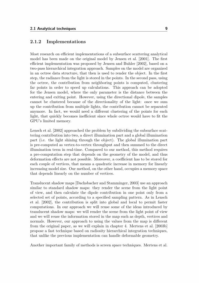
Most research on efficient implementations of a subsurface scattering analyticalmodel has been made on the original model by Jensen et al. [2001]. The firstefficient implementation was proposed by Jensen and Buhler [2002], based on atwo-pass hierarchical integration approach. Samples on the model are organizedin an octree data structure, that then is used to render the object. In the firststep, the radiance from the light is stored in the points. In the second pass, usingthe octree, the contribution from neighboring points is computed, clusteringfar points in order to speed up calculations. This approach can be adoptedfor the Jensen model, where the only parameter is the distance between theentering and exiting point. However, using the directional dipole, the samplescannot be clustered because of the directionality of the light: once we sumup the contribution from multiple lights, the contribution cannot be separatedanymore. In fact, we would need a different clustering of the points for eachlight, that quickly becomes inefficient since whole octree would have to fit theGPU’s limited memory.

Lensch et al. [2002] approached the problem by subdividing the subsurface scat-tering contribution into two, a direct illumination part and a global illuminationpart (i.e. the light shining through the object). The global illumination partis pre-computed as vertex-to-vertex throughput and then summed to the directillumination term in real-time. Compared to our method, this method requiresa pre-computation step that depends on the geometry of the model, and thusdeformation effects are not possible. Moreover, a coefficient has to be stored foreach couple of vertices, that means a quadratic increase in memory for linearlyincreasing model size. Our method, on the other hand, occupies a memory spacethat depends linearly on the number of vertices.

Translucent shadow maps [Dachsbacher and Stamminger, 2003] use an approachsimilar to standard shadow maps: they render the scene from the light pointof view, and then calculate the dipole contribution in one point only from aselected set of points, according to a specified sampling pattern. As in Lenschet al. [2002], the contribution is split into global and local to permit fastercomputations. In our approach we will reuse some of the ideas introduced bytranslucent shadow maps: we will render the scene from the light point of viewand we will reuse the information stored in the map such as depth, vertices andnormals. However, our approach to using the values from the map is differentfrom the original paper, as we will explain in chapter 4. Mertens et al. [2003b]propose a fast technique based on radiosity hierarchical integration techniques,that unlike the previous implementation can handle deformable geometry.

Another important family of methods is screen space techniques. Mertens et al.

10 Related Work

[2003a] propose an image space GPU technique that pre-computes a set of sam-ple points for the area integration and then performs the integral over multipleGPU passes. d’Eon et al. [2007], Eugene and David [2007] propose a methodin image-space, interpreting subsurface scattering as a sum of images blurredwith a gaussian filter. The gaussians are then weighted to fit the diffusion ap-proximation. Jimenez et al. [2009] improves further the technique, giving moreprecise results in the case of skin. All these techniques assume that the diffu-sion profile can be precomputed and then fitted with a sum of gaussians: as wehave already mentioned, this is not possible for the directional dipole, wherethe diffusion profile varies depending on the angle of incidence of the incomingray of light. Moreover, even if we were able to compute the coefficients for eachpossible combination of parameters, it would not be possible to apply a gaussianfilter with a kernel that varies per pixel.

Shah et al. [2009] present a fast screen space technique that render the objectas a series of splats, using GPU blending to sum over the various contributions.The diffusion profile in this case is pre-computed and stored as a texture. As inthe previous techniques, the directionality of the incoming light does not allowthe pre-computation of a diffusion profile. Moreover, the directional dipole isnot symmetrical, so the splats would have to use a bigger radius in order toaccount for all the contribution, increasing computation and blending costs.

2.2 Numerical techniques

Numerical techniques for subsurface scattering are often not specific, but comefor free or as an extension of a global illumination numerical approximation,since the governing equations are essentially the same. Given their generality,they are usually slower than their analytical counterpart, and often rely onheavy pre-computation steps in order to achieve interactive framerates. Thevolumetric version of Jensen’s Photon Mapping[Jensen and Christensen, 1998]was originally developed to render participating media in general, but it has beenadapted for subsurface scattering[Dorsey et al., 1999]. Classical approaches asa full Monte-Carlo simulation implementation of the light-material interaction,and finite-difference methods exist in literature[Stam, 1995].

Some less general methods have been introduced in order to devise more effi-cient approximations when it comes to subsurface scattering. Stam [1995] usesthe diffusion approximation with the finite difference method on the object dis-cretized on a 3D grid. Fattal [2009] uses as well a 3D grid, that is swept witha structure called light propagation map, that stores the intermediate resultsuntil the simulation is complete. All the numerical methods described so far are

2.2 Numerical techniques 11

not real-time, and they are generally not well-suited for a GPU environment.

Wang et al. [2010], instead of performing the simulation on a discretized 3D grid,makes the propagation directly in the mesh, converting it into a connected grid oftetrahedrons called QuadGraph. This grid can be optimized to be GPU cachefriendly, and provides a real-time rendering of not-deformable heterogeneousobjects. The problem in this method is that the QuadGraph is slow to compute(20 minutes for very complex meshes) and has heavy memory requirements forthe GPU. Compared to our method, this one requires an heavy pre-computationstep, and allows only not-deformable objects. However, as most of propagationtechniques, it can handle heterogeneous materials, while our method can not.

Precomputed radiance transfer methods are another class of general global illu-mination methods. These methods pre-compute part of the lighting and storeit in tables[Donner et al., 2009], allowing to retrieve it efficiently with an addi-tional memory cost. The problem with this methods compared to ours is that itsmemory requirements increase exponentially if we want to handle deformablematerials and changing light conditions. Moreover, it requires an heavy pre-computation in order to calculate the lighting coefficients. Our method, beinganalytical, does not required either a lot of memory or an heavy pre-computationstep.

A recent method called SSLPV (Subsurface Scattering Light Propagation Vol-umes) [Børlum et al., 2011] extends a technique originally developed by Ka-planyan and Dachsbacher [2010] to propagate light efficiently in a scene usinga set of discretized directions on a 3D grid. The method allows real-time exe-cution times and deformable meshes with no added pre-computation step, withthe drawback of not being physically accurate. Moreover, the required memoryspace on the GPU is larger than the one required than our method, since thevoxelization of the mesh must be stored.

Finally, for real-time critical applications (such as computer games), translu-cency is often estimated as a function of the thickness of the material, that isused to modify a lambertian term [Tomaszewska and Stefanowski, 2012, Green,2004]. The thickness is usually evaluated by sampling a depth map. A methodby Kosaka et al. [2012] uses an approach similar to the one we will describe in or-der to compute the thickness of the material using a different camera direction.While not physically accurate, this techniques allows to have a fast translucencyeffect that can be easily added to existing deferred pipelines. Compared to ourmethod, this method requires no storage space and light computation. However,the translucency effects are not represented faithfully, and some artifacts mayappear, as pointed out in Green [2004], and multi-sampling should be used inorder to avoid artifacts.

12 Related Work

As we can see, in the reviewed literature so far there is not a proper way toaccount for direction in subsurface scattering in real-time, or at least one thatsatisfies the requirements we have made in chapter 1. We will introduce indetail our method to handle directional subsurface scattering in real-time inchapter 4. In the next chapter, we are going to give a theoretical introductionto a mathematical description of light transport, as well as giving the properformulas and definition of the standard dipole model by Jensen et al. [2001] andthe directional dipole model presented by Frisvad et al. [2014].

Chapter 3

Theory

In this chapter, we give a theoretical introduction to the topic dealt with in thisthesis. The ultimate goal of this chapter is to introduce and describe analyticalmodels for subsurface scattering. First, we will give a brief introduction to thenature of light, and how we physically describe it. Secondly, we will introducethe basic radiometric quantities that will be used throughout the chapter. Then,we will describe how this quantities are related and can be used to describe light-material interaction, using reflectance functions, of which BSSRDF functions area special case. Finally, we will introduce subsurface scattering and the diffusionapproximation, concluding with a description of two BSSRDF models, by Jensenet al. [2001] and Frisvad et al. [2014].

14 Theory

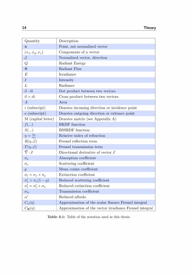
Quantity Descriptionx Point, not normalized vector(xx, xy, xz) Components of a vector~ω Normalized vector, directionQ Radiant EnergyΦ Radiant FluxE IrradianceI IntensityL Radiance~n · ~m Dot product between two vectors~n× ~m Cross product between two vectorsA Areai (subscript) Denotes incoming direction or incidence pointo (subscript) Denotes outgoing direction or exitance pointM (capital letter) Denotes matrix (see Appendix A)f(...) BRDF functionS(...) BSSRDF functionη = n1

n2Relative index of refraction

R(η, ~ω) Fresnel reflection termT (η, ~ω) Fresnel transmission term~∇ · ~x Directional derivative of vector ~xσa Absorption coefficientσs Scattering coefficientg Mean cosine coefficientσt = σs + σa Extinction coefficientσ′s = σs(1− g) Reduced scattering coefficientσ′t = σ′t + σa Reduced extinction coefficientσtr Transmission coefficientα′ Reduced albedoCφ(η) Approximation of the scalar fluence Fresnel integralCE(η) Approximation of the vector irradiance Fresnel integral

Table 3.1: Table of the notation used in this thesis.

3.1 Light and Radiometry 15

3.1 Light and Radiometry

Light is a form of electromagnetic radiation, that propagates through space asa sinusoidal wave. Usually by light we refer to visible light, the small part ofthe electromagnetic spectrum the human eye is sensible to (see Figure 3.1).This small window is between the 380 nm of infrared and 750 nm of ultravioletlight, but the precise boundaries may vary according to the environment andthe observer. Instead explicitly noted, we will use the terms light and visiblelight interchangeably in this report.

The study of light is usually referred as optics. In computer aided image syn-thesis, we are interested in representing faithfully how visible light propagateshow it interacts with the objects and the materials in a scene. In addition, weare interested in lighting effects that are noticeable at human scales (1 mm -1 km), like subsurface scattering, absorption and emission phenomena. Opticsstudies more effects, like diffraction, interference and quantum effects, but weare not interested in representing them because for visible light they happen ona microscopic scale (1 nm - 1 µm).

380

450

570

620

750

1000zm 100zm 10zm 1zm 10zcm 1zcm 1zmm 100zµm 10zµm 1zµm 100znm 10znm 1znm

1019101810171016101510141013101210111010109108107106

Wavelengthfmd

FrequencyfHzd

Longzwaves Microwaves Infrared Ultraviolet Gammazrays

Visiblezlight

Figure 3.1: The electromagnetic spectrum.

The branch of physics that studies how to measure electromagnetic radiationis called radiometry. The energy of light, like all the others forms of energy,is measured in Joules [J = kg m s−2], and its power in Watts [W = kg m s−3].Photometry, on the other hand, measures electromagnetic radiation as it is

16 Theory

perceived from the human eye, and limits itself only to the visible spectrum,while radiometry spans all of it. The corresponding names for energy and powerin photometry are radiant energy, measured in talbots [cd s], and radiant flux,measured in candelas [cd].

In image synthesis it is more common to use radiometry, as its quantities di-rectly derive from the electromagnetic theories, are universal, and can be easilyconverted to the photometric ones when necessary. The most important radio-metric quantities used in computer graphics are radiant flux, radiant energy,radiance, irradiance and intensity.

3.2 Radiometric quantities

3.2.1 Radiant flux

The radiant flux, also known as radiant power, is the most basic quantity inradiometry. It is usually indicated with the letter Φ and it is measured in joulesper seconds [J s−1] or Watts [W]. The quantity indicates how much power thelight irradiates per unit time.

3.2.2 Radiant energy

Radiant energy, usually indicated as Q, is the energy that the light carries ina certain amount of time. Like all the other SI units for energy, it is measuredin joules [J]. Radiant energy is obtained integrating the radiant flux along timefor an interval ∆T :

Q =∫

∆TΦ(t) dt

Due to the dual nature of the light, the energy carried by the light can be derivedboth considering light as made of particles, called photons, or considering it asa wave. We will not dig further into the topic, because for rendering purposesis not important if we characterize light as a flux of particles or as a sinusoidalwave.

3.2 Radiometric quantities 17

3.2.3 Irradiance

Irradiance, usually defined as E, is the radiometric unit that measures the ra-diant flux per unit area falling on a surface. It is measured in Watts per squaremeter [W m−2]. It is defined as the flux per unit area:

E = dΦdA

Irradiance is usually the term in literature used for the incoming power per unitarea. The converse, i.e. the irradiance leaving a surface, it is usually referred asradiant exitance or radiosity, and indicated with the letter B.

B

A

Figure 3.2: Irradiance versus power. For the two surfaces A and B, the receivedpower Φ is the same, while the two irradiances EA and EB are different,as the area of B is twice as the one of A.

3.2.4 Intensity

Intensity is defined as the differential radiant flux per differential solid angle:

I(~ω) = dΦdω

(3.1)

It is measured in Watts per steradian [W sr−1] and it is indicated with the letterI. Intensity is often a misused term in the physics community, as it is used formany different quantities. Depending on the research community, intensity mayrefer to irradiance or even to radiance (see the following section). The definitiongiven in 3.1 we use the most common definition given by the optics community.

18 Theory

3.2.5 Radiance

Radiance is arguably the most important quantity in image synthesis. It is de-fined precisely as the differential of the flux per solid angle per projected surfacearea, and it is measured in Watt per steradian per square meter [W sr−1 m].

L(~ω) = d2ΦdωdA cos θ

Where θ is the angle between the surface normal and the incoming ray of light(so that cos θ = ~n · ~ωi).

Figure 3.3: Radiance. The element of area dA gets projected according to the angleθ = cos−1 ~n · ~ω. Then the incoming flux Φ gets divided by the projectedarea and by the solid angle subtended by it.

Radiance has the important property of being constant along a ray of light. Inaddition, the sensibility of the human eye to light is directly proportional tothe radiance. For a discussion on why radiance is related to the sensitivity ofsensors and the human eye, see Cohen et al. [1993].

3.3 Reflectance Functions 19

All the other radiometric quantities can be derived from radiance:

E =∫

2πLi(~ω) cos θ dω

B =∫

2πLo(~ω) cos θ dω

I(~ω) =∫A

L(~ω) cos θ dA

Φ =∫A

∫2πL(~ω) cos θ dωdA

(3.2)

For simplicity of notation, the dependence from the point of incidence x hasbeen dropped in equations 3.2.

3.2.6 Radiometric quantities for simple lights

To help with the formulas used later in the report, we derive the standardradiometric quantities for the two simplest types of light, i.e. directional andpoint lights.

• Directional lights simulate very distant light sources, in which all the raysof light are parallel (e.g. sunlight). They are represented by a direction~ωl and a constant radiance value, L.

• Point lights simulate lights closer to the observer. Isotropic point lightsare represented by a position of the light xl and a constant intensity I.Point lights have a falloff that depends on the inverse square law, i.e. theradiance diminishes with the square of the distance.

Table 3.2 shows different radiometric quantities evaluated for point and direc-tional lights, for a surface point x with surface normal ~n.

3.3 Reflectance Functions

After introducing the basic radiometric quantities, we still lack a way to describelight material interaction. More precisely, we need a way to relate the incomingand the outgoing radiance on a point of a chosen surface.

20 Theory

Quantity Directional light Point light

Cosine term cos θ = ~n · ~ωl cos θ = (x−xl)·~n|x−xl|

Φ(x) Flux L δ( ~ω) 4πI

E(x) Irradiance L cos θ I cos θ|xl−x|2

I(x, ~ω) Intensity L δ(~ω) I

L(x, ~ω) Radiance L δ(~ω) I|xl−x|2

Table 3.2: Different radiometric values for simple light sources.

3.3.1 BRDF functions

One of the possible way to describe light-material interaction is by using aBDRF function [Nicodemus et al., 1992], acronym for Bidirectional ReflectanceDistribution Function. The BRDF function f(x, ~ωi, ~ωo) is defined on one pointx of the surface as the differential ratio between the exiting radiance and theirradiance:

f(x, ~ωi, ~ωo) = dLo(x, ~ωo)dEi(x, ~ωi)

= dLo(x, ~ωo)Li(x, ~ωi) cos θid~ωi

(3.3)

The BRDF states that the incoming and the outgoing radiance are proportional,so that the energy hitting the material at the point x is proportional to theenergy coming out from the point. BRDF functions have generally the followingproperties:

• reciprocal: for the Hemholtz reciprocity principle, a physics result that isalso the basis of reverse path ray tracing [Desolneux et al., 2007]:

f(x, ~ωi, ~ωo) = f(x, ~ωo, ~ωi)

• anisotropic: if the surface changes orientation and ~ωi and ~ωo stays thesame, the resulting BRDFs are different. So generally

f(x, ~ωi, ~ωo) 6= f(x, R~ωo, R~ωi)

where R is a rotation matrix with arbitrary axis around the point x.

• positive, since the BRDF regulates the transport between two positivequantities (radiance, irradiance).

f(x, ~ωo, ~ωi) ≥ 0

3.3 Reflectance Functions 21

• energy conserving, so that the energy of the outgoing ray is no grater thatthe one of the incoming one∫

2πf(x, ~ωo, ~ωi) cos θod~ωo ≤ 1

By inverting equation 3.3, we obtain the so-called reflectance equation:

Lo(x, ~ωo) =∫

2πf(x, ~ωi, ~ωo)Li(x, ~ωi) cos θid~ωi

Later we will use this equation as a starting point to obtain a formulation ofthe full rendering equation. The BRDF function has some limitations, beingnot able to account for all phenomena. For example, with a BRDF it is notpossible to account for subsurface scattering, because it assumes the light entersand leaves the material at the same point. To model these phenomena, morecomplicated functions are needed, like the BSSRDF function described later inthis chapter.

Figure 3.4: Setup for a BRDF. Note that the light enters and leaves the surface atthe same point.

3.3.2 Examples of BRDF functions

There are many examples of BRDF functions in literature. In this section, inorder to illustrate some examples, we will introduce three of them: the lamber-tian or diffuse BRDF, the specular or mirror BRDF and glossy BRDFs. For adetailed overview on BRDF functions, refer to [Akenine-Moller et al., 2008].

22 Theory

(a) Lambertian BRDF (b) Mirror BRDF

(c) Glossy BRDF (d) Combined BRDF

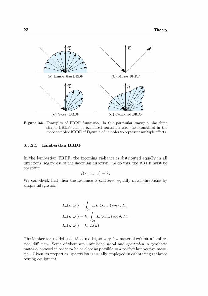
Figure 3.5: Examples of BRDF functions. In this particular example, the threesimple BRDFs can be evaluated separately and then combined in themore complex BRDF of Figure 3.5d in order to represent multiple effects.

3.3.2.1 Lambertian BRDF

In the lambertian BRDF, the incoming radiance is distributed equally in alldirections, regardless of the incoming direction. To do this, the BRDF must beconstant:

f(x, ~ωi, ~ωo) = kd

We can check that then the radiance is scattered equally in all directions bysimple integration:

Lo(x, ~ωo) =∫

2πfdLi(x, ~ωi) cos θid~ωi

Lo(x, ~ωo) = kd

∫2πLi(x, ~ωi) cos θid~ωi

Lo(x, ~ωo) = kd E(x)

The lambertian model is an ideal model, so very few material exhibit a lamber-tian diffusion. Some of them are unfinished wood and spectralon, a syntheticmaterial created in order to be as close as possible to a perfect lambertian mate-rial. Given its properties, spectralon is usually employed in calibrating radiancetesting equipment.

3.3 Reflectance Functions 23

3.3.2.2 Mirror BRDF

Another simple kind of BRDF is the perfectly specular BRDF, or mirror BRDF.In this function, all the incoming radiance from one direction ~ωi is transferredtowards the reflected direction ~ωr, defined as ~ωr = ~ωi−2(~ωi ·~n)~n. The resultingBRDF is defined as follows:

f(x, ~ωi, ~ωo) = δ(~ωo − ~ωr)cos θi

The function δ(~ω) is a hemispheric delta function. Once integrated over a hemi-sphere, the function evaluates to one only for the vector ~ω = 0. Putting theBRDF into the reflectance equation gives the following outgoing radiance:

Lo(x, ~ωo) ={Li(x, ~ωi) if ~ωo = ~ωr

0 otherwise

that is the expected result, as all the radiance is reflected into the direction ~ωr.

3.3.2.3 Glossy BRDFs

As we can see from real life experience, rarely objects are completely diffuse orcompletely specular. These two models are idealized models, that represent anideal case. So, to create a realistic BRDF model, we often need to combine thetwo terms and add an additional one, called glossy reflection.

The most used BRDF model used to model glossy reflections is based on micro-facet theory [Torrance and Sparrow, 1992, Ashikmin et al., 2000] and was firstintroduced by [Blinn, 1977]. In this theory, the surface of an object is modeledas composed of small mirrors. In one of its classical formulations, the BRDF isrepresented as:

f(x, ~ωi, ~ωo) = DGR

4 cos θr cos θi= GR

4(~n · ~h)s

(~n · ~r)(~n · ~ωi)

D regulates how microfacets are distributed, and it is often modeled as (~n ·~h)s,where ~h is the half vector between the eye and the light, and s is an attenuationparameter. ~h is defined as:

~h = ~ωo + ~ωi‖~ωo + ~ωi‖

G accounts for the object self shadowing, while R is the Fresnel reflection term(more details in Section 3.3.4). ~r is the reflection vector as defined in the previous

24 Theory

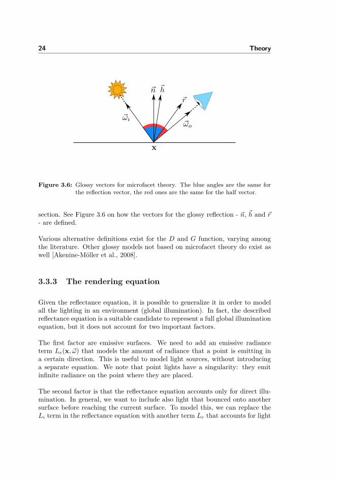
Figure 3.6: Glossy vectors for microfacet theory. The blue angles are the same forthe reflection vector, the red ones are the same for the half vector.

section. See Figure 3.6 on how the vectors for the glossy reflection - ~n, ~h and ~r- are defined.

Various alternative definitions exist for the D and G function, varying amongthe literature. Other glossy models not based on microfacet theory do exist aswell [Akenine-Moller et al., 2008].

3.3.3 The rendering equation

Given the reflectance equation, it is possible to generalize it in order to modelall the lighting in an environment (global illumination). In fact, the describedreflectance equation is a suitable candidate to represent a full global illuminationequation, but it does not account for two important factors.

The first factor are emissive surfaces. We need to add an emissive radianceterm Le(x, ~ω) that models the amount of radiance that a point is emitting ina certain direction. This is useful to model light sources, without introducinga separate equation. We note that point lights have a singularity: they emitinfinite radiance on the point where they are placed.

The second factor is that the reflectance equation accounts only for direct illu-mination. In general, we want to include also light that bounced onto anothersurface before reaching the current surface. To model this, we can replace theLi term in the reflectance equation with another term Lr that accounts for light

3.3 Reflectance Functions 25

coming from another surface. This term can be usually modeled as the productof the radiance of the light plus a visibility function V (x).

Accounting for all the described factors, we reach one formulation of the ren-dering equation [Kajiya, 1986]:

Lo(x, ~ωo) = Le(x, ~ω) +∫

2πf(x, ~ωi, ~ωo)Li(x, ~ωi)V (x) cos θid~ωi

This form of the rendering equation is still not completely general, since itis based on a BRDF, to it comes with the same limitations (no subsurfacescattering effects or wavelength-changing effects like iridescence). We will extendthe rendering equation in order to account for these phenomena later on in thischapter.

3.3.4 Fresnel equations

Until now, on the described BRDF models, we did consider only the reflectedpart of the radiance. When a beam of light coming from direction ~ωi hits asurface, only part of the incoming radiance gets reflected, while another partgets refracted into the material. As we can see from Figure 3.7, we obtain thetwo vectors ~ωr and ~ωt, the reflected and refracted vector, defined as follows [Kayand Greenberg, 1979]:

~ωr = ~ωi − 2(~ωi · ~n)~n~ωt = η((~ωi · ~n)~n− ~ωi)− ~n

√1− η2(1− (~ωi · ~n)2)

Where η = n1n2

is the relative index of refraction between the two materials.With this setup, illustrated in Figure 3.7, we can use a solution to Maxwell’sequations for wave propagation to describe the radiant flux. In particular, wecan tell which part of the power propagates in the reflected and refracted direc-tion respectively. The coefficients that describe this subdivision of the power arecalled Fresnel coefficients [Born and Emil, 1999]. The coefficients are differentaccording to the polarization of the incoming light (parallel or perpendicular),

26 Theory

Figure 3.7: Reflected and refracted vector on mismatching indices of refraction.

so there are two for reflection (Rs, Rp) and two for transmission (Ts, Tp).

Rs(η, ~ωi) =∣∣∣∣η cos θi − cos θtη cos θi + cos θt

∣∣∣∣2Rp(η, ~ωi) =

∣∣∣∣η cos θt − cos θiη cos θt + cos θi

∣∣∣∣2Ts(η, ~ωi) = η

cos θtcos θi

∣∣∣∣ 2 cos θiη cos θi + cos θt

∣∣∣∣2Tp(η, ~ωi) = η

cos θtcos θi

∣∣∣∣ 2 cos θiη cos θt + cos θi

∣∣∣∣2In most computer graphics applications (and this is reasonable for most of thereal-world lights), we assume that the two polarizations are equally mixed. So,we will use the coefficient R = Rs+Rp

2 and T = Ts+Tp2 in our calculations. Note

that R+ T = 1, so the overall energy is conserved.

3.3.5 BSSRDF functions and generalized rendering equa-tion

As we anticipated in Section 3.3.1, the BRDF theory that was introduced beforeis not accurate in predicting the behavior for all materials, since BRDF modelsassume that the light enters and leaves the material in the same point. Whilethis assumption holds true for a wide range of material, like metal or plastic, it

3.3 Reflectance Functions 27

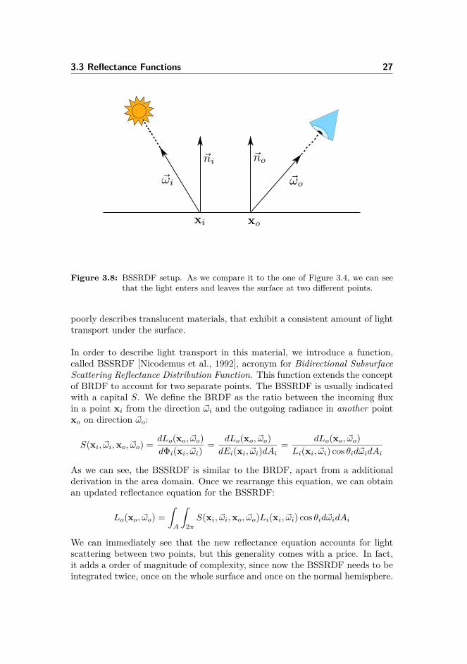
Figure 3.8: BSSRDF setup. As we compare it to the one of Figure 3.4, we can seethat the light enters and leaves the surface at two different points.

poorly describes translucent materials, that exhibit a consistent amount of lighttransport under the surface.

In order to describe light transport in this material, we introduce a function,called BSSRDF [Nicodemus et al., 1992], acronym for Bidirectional SubsurfaceScattering Reflectance Distribution Function. This function extends the conceptof BRDF to account for two separate points. The BSSRDF is usually indicatedwith a capital S. We define the BRDF as the ratio between the incoming fluxin a point xi from the direction ~ωi and the outgoing radiance in another pointxo on direction ~ωo:

S(xi, ~ωi,xo, ~ωo) = dLo(xo, ~ωo)dΦi(xi, ~ωi)

= dLo(xo, ~ωo)dEi(xi, ~ωi)dAi

= dLo(xo, ~ωo)Li(xi, ~ωi) cos θid~ωidAi

As we can see, the BSSRDF is similar to the BRDF, apart from a additionalderivation in the area domain. Once we rearrange this equation, we can obtainan updated reflectance equation for the BSSRDF:

Lo(xo, ~ωo) =∫A

∫2πS(xi, ~ωi,xo, ~ωo)Li(xi, ~ωi) cos θid~ωidAi

We can immediately see that the new reflectance equation accounts for lightscattering between two points, but this generality comes with a price. In fact,it adds a order of magnitude of complexity, since now the BSSRDF needs to beintegrated twice, once on the whole surface and once on the normal hemisphere.

28 Theory

As we did for the BRDF, we can further extend the reflectance equation tofurther include visibility and emission, giving an extended form of the renderingequation [Jensen et al., 2001].

Lo(xo, ~ωo) = Le(xi, ~ωi) +∫A

∫2πS(xi, ~ωi,xo, ~ωo)Li(xi, ~ωi)V (x)(~n · ~ωi)d~ωidAi

(3.4)From now on, by ‘rendering equation’ in this report we will mean the one inequation 3.4.

3.4 Light transport and subsurface scattering

When we derive our models for lighting, in general we assume that the light istraveling in vacuum. This assumption holds for light that is propagating thoughthe air (which is assimilable to vacuum), but once we relax it, more variablesshould be taken into consideration. Objects through which light travels are re-ferred as participating media. In this chapter, we will derive and consider analternative formulation of the rendering equation for light traveling into partic-ipating media, called radiative transfer equation [Chandrasekar, 1950].

When a beam of light travels through an object, various phenomena occur. Aphoton on the beam can be either being absorbed (disappear), scattered (changedirection) or emitted (appear). These phenomena can be uniform throughoutthe material (homogeneous materials), as in solid materials like wax or leaves,or be not uniform (heterogeneous materials), like in smoke or clouds.

We will briefly describe all three mentioned effects, then combine them to com-pose the radiative transfer equation. The purpose is to describe how radiancevaries along a beam of light with direction ~ω. This directional derivative isindicated as:

(~∇ · ~ω)L(x, ~ω) = ∂Lx∂x

~ωx + ∂Ly∂y

~ωy + ∂Lz∂z

~ωz

3.4.1 Emission

Emission is the natural property of the materials to emit light, i.e. to generatephotons that add to the existing ones passing through the material. The effectis generally generated by chemical processes emitting photons (as in fireflies),by natural black-body radiation emission in the visible spectrum (such as in a

3.4 Light transport and subsurface scattering 29

(a) Emission

x(b) Absorption

(c) Out Scattering (d) In Scattering

star like the sun or in incandescent bulbs), or by other radiation that changesits wavelength into the visible spectrum.

In the directional 3D derivative, the variance in emission is modeled as a constantdepending only on the current position and direction:

(~∇ · ~ω)L(x, ~ω) = ε(x, ~ω)

This means that emission increases linearly along the body: if the beam travelsa distance d within the medium, d ·k photons are emitted. Emission is generallyisotropic, not depending on the direction (ε(x, ~ω) = ε(x)).

3.4.2 Absorption

Absorption is a property of materials that describes a simple physical phe-nomenon: a photon, traveling though the material, hits one atom of the material.The energy carried by the photon is then absorbed by the atom, augmenting itskinetic energy. This directly translates in an increase of heat in the material.Usually, a certain percentage of the photons that hit the atoms is absorbed perunit length. Then, if k is the percentage of the photons absorbed in a meter,after one meter the original radiance will become k · Li, then k2 · Li, etc.

If we write this phenomena as a differential equation, we get after a distance da radiance reduction of kd = e−σad, that leads to the following 3D directionalderivative:

(~∇ · ~ω)L(x, ~ω) = −σa(x, ~ω)L(x, ~ω)

30 Theory

σa is referred as the absorption coefficient. Also this coefficient is genericallyisotropic, and constant for homogenous materials.

3.4.3 Out-scattering

Out scattering is the radiance lost due to scattering. The scattering phenomenonhappens when photons are deflected away from the current direction ~ω. As inthe previous case, the phenomena is modeled as a percentage of the radiancelost per unit length. So the loss due to out-scattering is modeled as:

(~∇ · ~ω)L(x, ~ω) = −σs(x, ~ω)L(x, ~ω)

σs is referred as the scattering coefficient. We note that in this case we arenot interested in which direction the photons are actually going. That will beaccounted in the in-scattering term of another point in the material.

3.4.4 In-scattering

Given some loss due to some of the photons changing direction, there will besome of them that from other scattering events will change to the ~ω direction.We need then to discover the number of photons that comes from all the otherdirections. To do this, we integrate the incoming radiance from all directions inthe point x. This quantity, similar to irradiance, in an infinite medium is calledfluence, and indicated as φ:

φ(x) =∫

4πL(x, ~ω′)dω′

Fluence should be then averaged over the entire sphere, yielding φ4π as a normal-

ization factor. This quantity then is then multiplied by the scattering coefficient,because only some photons on average scatter towards the current point. Thisresults in:

(~∇ · ~ω)L(x, ~ω) = σs(x) 14π

∫4πL(x, ~ω′)dω′ (3.5)

However, equation 3.5 assumes that radiance scatters equally in all directions.This is not usually the case, and the 1

4π term needs to be replaced by a probabil-ity distribution function that describes how the photons scatter in the medium.This function is called phase function, and indicated as p(x, ~ω, ~ω′). In the actualmodels its integral on the hemisphere is often used as a parameter, called meancosine (g):

g(x) =∫

4πp(x, ~ω, ~ω′)~ω · ~ω′dω′

3.4 Light transport and subsurface scattering 31

This term indicates the general direction of the scattering in the material. Ifpositive, the scattering is prevalent along the beam (forward scattering), if neg-ative is prevalent in the opposite direction (backward scattering). If zero, thescattering is isotropic, i.e. equal in all directions.

So, the final 3D equation for in-scattering, accounting for the phase function, isas follows:

(~∇ · ~ω)L(x, ~ω) = σs(x)∫

4πp(x, ~ω, ~ω′)L(x, ~ω′)dω′

3.4.5 Final formulation of the radiative transfer equation

Combining emission, absorption, scattering described in the previous sections,we reach the final formulation of the radiative transfer equation (RTE):

(~∇ · ~ω)L(x, ~ω) = −σt(x)L(x, ~ω) + ε(x) + σs(x)∫

4πp(x, ~ω, ~ω′)L(x, ~ω′)dω′ (3.6)

Where the two reducing term, scattering and absorption, have been combinedtogether in σt = σa + σs, called the extinction coefficient.

3.4.6 The diffusion approximation

The radiative transfer equation 3.6 is a integro-differential equation with manydegrees of freedom. As we stated in Chapter 2, there are rendering techniquesthat numerically solve the equation in order to obtain a realistic result. However,analytical methods tend to use some approximations of the RTE, that hold wellgiven specific conditions. The diffusion approximation [Ishimaru, 1997] is oneof these approximations, and it is still widely used today since its introductionin the computer graphics community by [Stam, 1995].

The assumption under the diffusion approximation is that given a physicalmedium, the number of scattering events is so high that the beam of lightquickly becomes isotropic. Each one of the scattering events blurs the light dis-tribution, and as a result the distribution becomes more uniform as the numberof scattering events increases. This has been proven to be a reasonable assump-tion even for highly anisotropic light sources (e.g. a focused laser beam) andphase functions.

When using the diffusion approximation, instead of using the extinction coeffi-cient σt, we account for the contribution from the phase function by using the

32 Theory

so-called reduced extinction coefficient σ′t. It is defined as σ′t = σa + σ′s, withσ′s = σs(1 − g). σ′s Is called reduced scattering coefficient. The converse of thereduced extinction coefficient is called mean free path and represents the averagedistance that light travels in the medium before being absorbed or scattered.

The rationale behind this reduced coefficient is that a highly forward scatteringmaterial is virtually indistinguishable from a not-scattering material. So, forhighly forward scattering materials (g ≈ 1) the scattering coefficients reduceto zero. For highly backward scattering materials (g ≈ −1), the scattering isaccounted for twice as for an isotropic material (see table 3.3).

Coefficient BackwardScattering(g ≈ −1)

Isotropic

(g ≈ 0)

ForwardScattering(g ≈ 1)

σ′s 2σs σs 0

σ′t σa + 2σs σa + σs σa

Table 3.3: Explicit scattering coefficients for different kinds of materials.

We leave to Ishimaru [1997] and Jensen et al. [2001] for the algebraic details ofthe calculation. Once we solve the diffusion equation, we obtain the followingformula for φ(x), the fluence of light in an infinite scattering medium.

φ(x) = Φ4πD

eσtrr

r(3.7)

We recall that φ(x) =∫

4π L(x, ~ω)d~ω. r = ‖x‖ is the distance from the point tothe light source. The two coefficients D and σtr are called diffusion coefficientand transmission coefficient respectively. The two coefficients are defined asfollows:

D = 13σ′t

σtr =√

3σaσ′t =√σaD

This is the equation describe light propagation in an infinite medium, i.e. no sur-face interaction is considered. In order to derive an actual BSSRDF model fromthe diffusion approximation, boundary conditions must be considered. JensenJensen et al. [2001] derived an analytical model starting from this approxima-tion of the RTE, while Frisvad Frisvad et al. [2014] uses a higher order diffusionapproximation of the RTE. The two models are explained in the following sec-tions.

3.4 Light transport and subsurface scattering 33

3.4.7 Standard dipole model

The first model we describe is due to Jensen et al. [2001]. It it usually referredin literature as Jensen dipole model or Standard dipole model. In their origi-nal paper, the authors used the diffusion approximation for light in an infinitemedium. Starting from that, they derive an approximation that holds for lightin a semi-infinite medium, i.e. light traveling in void hitting a planar slab of atranslucent material.

As a boundary condition, we take the light coming out of the material. Lightcoming out of the material has a initial fluence φ0. We assume then that thefluence decays linearly until a distance z = 2AD from the surface, where itbecomes zero. See Donner [2006] for the full derivation. D is the diffusioncoefficient, while A is a corrective term that accounts for mismatching indicesof refraction:

A = 1 + Fdr1− Fdr

Fdr =∫

2πR(η, ~n · ~ω)(~n · ~ω)d~ω

(3.8)

Where R is the Fresnel reflection term as defined in Section 3.3.4, and η = n1/n2is the relative refraction index. The Fresnel reflectance integral Fdr is usuallyapproximated with an analytical expression:

Fdr = −1.440η2 + 0.710

η+ 0.668 + 0.0036η

Given the boundary condition, we can then model the subsurface scattering ina point xo with two small sources on the point, a configuration called a dipole.One source is placed beneath the surface, called the real source, while the otherone is mirrored above the surface, called virtual source. The first source actuallymodels the subsurface scattering effect, while the second one reduces the first inorder to account for the boundary conditions and the extrapolation boundary.Refer to Figure 3.9 for a visual detail on the setup.

The real source is placed one mean free path beneath the surface, at zr =1/σ′t, while the virtual one is placed symmetrically according to the boundaryconditions, ad a distance zv = zr + 4AD. From zr and zv we can calculate thedistances dr and dv from the entrance point xi. Given r = ‖xo−xi‖, we obtain:

dr =√z2r + r2

dv =√z2v + r2

34 Theory

Figure 3.9: Setup for the standard dipole model.

Given these constraints, we obtain an equation for the BSSRDF in a semi infinitemedium:

Sd(xi, ~ωi,xi, ~ωo) = α′

4π2

[zr(1 + σtrdr) e−σtrdr

d3r

+ zv(1 + σtrdv) e−σtrdvd3v

]Where α′ = σ′s/σ

′t is called reduced albedo.

The model so far described was intended to model only the multiple scatteringBSSRDF term, Sd. In order to obtain the full BSSRDF S, a single scatteringterm S(1) must be added. Moreover, we need to add as well the two Fresneltransmission terms, one for the incoming and one for the outgoing radiance.There are in literature many approaches to model single scattering, that are outof the scope of this report. The final BSSRDF equation for the standard dipolemodel then becomes:

S(xi, ~ωi,xo, ~ωo) = T (η, ~ωi)Sd(xi, ~ωi,xo, ~ωo)T (η, ~ωo) + S(1)(xi, ~ωi,xo, ~ωo)

Jensen et al. [2001] in their original paper describes some corrections that needto be done to the model in order to make it work with generic surfaces, and onhow to account for extensions like texture support. We will not describe theseextensions here, remanding to the original paper for a detailed description.

3.4 Light transport and subsurface scattering 35

3.4.8 Directional dipole model

Various evolutions to the standard dipole model have been proposed through-out the years. In this chapter, we will introduce the BSSRDF approximationcalled directional dipole, proposed by Frisvad et al. [2014]. In the standarddipole model, in fact, the diffusive part of the BSSRDF depends only on thedistance between the point of incidence and the point of emergence, that isSd(xi, ~ωi,xo, ~ωo) = Sd(‖xo − xi‖).

The directional dipole model, based on the diffusion approximation, accountsfor the direction of the incoming light in its calculations, in order to model thescattering effects more precisely. Moreover, the model, instead of splitting theBSSRDF in a multiple and single scattering term, splits the BSSRDF into adiffusive term Sd and a term SδE , called reduced intensity, that can be com-puted using the delta-Eddington approximationJoseph et al. [1976]. The finalBSSRDF thus becomes:

S(xi, ~ωi,xo, ~ωo) = T (η, ~ωi)(Sd(xi, ~ωi,xo) + SδE(xi, ~ωi,xo, ~ωo))T (η, ~ωo) (3.9)

Where T are the Fresnel transmission coefficients for the incoming and outgoingdirections. We note also that the diffusive part of the BSSRDF does not dependon the outgoing direction ~ωo.

Diffusive BSSRDFThe diffusive part of the directional dipole model uses a first-order approxima-tion of the RTE, that for a point light in an infinite medium gives the followingfluence:

φ(xo, θ) = Φ4πD

eσtrr

r

(1 + 3D1 + σtrr

rcos θ

)(3.10)

WhereD and σtr are the two scattering coefficients defined beforehand, r = ‖xo‖and

cos θ = x · ~ω12

r

Where ~ω12 is the refracted vector as defined in Section 3.3.4. Comparing 3.10with equation 3.7, we can see that we introduced a new term that depends on theangle θ between the refracted incoming light vector and the vector connectingincidence and emergence.

Using the diffusion approximation, we can first establish a relationship betweenthe radiant exitance M(xo) and the diffusive BSSRDF S′d in an infinite medium:

dM(xo)dΦi(x, ~ωi)

= T (η, ~ωi)S′d(xi, ~ωi,xo) 4πCφ(1/η) (3.11)

36 Theory

Figure 3.10: Setup for the directional dipole model.

Where Cφ(1/η) is related to the integral on the hemisphere of the fresnel coeffi-cients. Using the definition of radiant exitance and inserting inside the classicaldiffusion approximation, we reach the diffusion formulation of the radiant exi-tance:

M(xo) = Cφ(η)φ(xo) + CE(η)D~no · ∇φ(xo) (3.12)

Again, Cφ(η) and CE(η) are two terms that are related to the integration of thefresnel coefficients. Combining the three equations 3.10, 3.11 and 3.12, we reachthe final form for our diffusive BSSRDF in an infinite medium:

S′d(x, ~ω12, r) = 14Cφ(1/η)

14π2

e−σtrr

r3[Cφ(η)

(r2

D+ 3(1 + σtrr)x · ~ω12

)−

− CE(η)(

3D(1 + σtrr) ~ω12 · ~no−

−(

(1 + σtrr) + 3D3(1 + σtrr) + (σtrr)2

r2 x · ~ω12

)x · ~no

)](3.13)

3.4 Light transport and subsurface scattering 37

Fresnel integrals

The two terms Cφ(η) and CE(η) originally come from integrating theoutgoing Fresnel transmittance over the whole outgoing hemisphere,weighted with a cosine term. The two functions are defined as follows:

Cφ(η) = 14π

∫2πT (η, ~ω)(~no · ~ω)d~ω

CE(η) = 34π

∫2πT (η, ~ω)(~no · ~ω)2d~ω

(3.14)

These two integrals can be rearranged in order to express them in termsof reflectance instead of transmittance, recalling R = 1− T .

Cφ(η) = 14π

(π −

∫2πR(η, ~ω)(~no · ~ω)d~ω

)= 1

4(1− 2C1)

CE(η) = 34π

(2π3 −

∫2πR(η, ~ω)(~no · ~ω)d~ω

)= 1

2(1− 3C2)(3.15)

Even with this rearrangement the integrals cannot be expressed in closedform. D’Eon and Irving [2011] use a convenient polynomial approxima-tion for the two coefficients C1 and C2, expressed as:

2C1 ≈

+0.919317− 3.4793η + 6.75335η2 − 7.80989η3

+4.98554η4 − 1.36881η5 η < 1−9.23372 + 22.2272η − 20.9292η2 + 10.2291η3

−2.54396η4 + 0.254913η5 η ≥ 1

3C2 ≈

0.828421− 2.62051η + 3.36231η2 − 1.95284η3

+0.236494η4 + 0.145787η5 η < 1−1641.1 + 135.926

η3 − 656.175η2 + 1376.53

η + 1213.67η−568.556η2 + 164.798η3

−27.0181η4 + 1.91826η5 η ≥ 1.

Boundary conditions

As the name implies, also for the directional dipole we model the boundaryconditions on the material interface using a dipole. In this case, however, insteadof using two point light sources, we use two ray sources, a real and a virtualone. As in the standard dipole, the source is displaced towards the normal of a

38 Theory

distance de. In the case of the standard dipole, we use 2D, that becomes 2ADin the case of mismatching indices of refraction on the interface. In the case ofthe directional dipole, we use

de = 2.131D√α′

Where we recall α′ = σ′s/σ′t as the reduced albedo. This result have been

proven [Davison and Sykes, 1958] to be consistent with numerical simulationsof the RTE. In addition, the A term is modified using the hemispheric Fresnelintegrals:

A(η) = 1− CE(η)2Cφ(η)

As the standard dipole, the directional dipole assumes a semi-infinite mediumgiven the previous boundary conditions. In order to relax this assumptions,we need to further extend the model in order to reduce undesired effects. Onefirst modification proposed by Frisvad et al. [2014] is to use a modified tangentplane defined by the normal ~n∗i to mirror the real source towards the mirrorlight source, instead of the obvious one defined by ~ni. We define the modifiednormal as follows:

~n∗i =

~ni for xo = xi

xo − xi‖xo − xi‖

× ~ni × (xo − xi)‖~ni × (xo − xi)‖

otherwise

Another important modification is the distance to the real source. In the stan-dard dipole, we used dr =

√z2r + r2, with zr = 1/σ′t, which is the average

distance a photon travels within the material before being absorbed or scat-tered. The problem of this definition is that it introduces a singularity in r = 0.Moreover, the standard dipole becomes fairly imprecise when r is small, over-estimating the overall effect. In order to avoid these problems, Frisvad et al.[2014] proposed a more complicated definition of dr that matches simulations oftransport theory more closely. For the details, see Appendix B in the originalpaper. dr is defined as follows, recalling σt = σs + σa:

d2r =

r2 +Dµ0(Dµ0 − 2de cosβ) µ0 ≥ 0 (frontlit)

r2 + 1(3σt)2 µ0 < 0 (backlit)

Where µ0 = −~ω12 · ~no is an indicator if the point xo is frontlit or backlit. β isa geometry term that is evaluated as:

cosβ = −

√r2 − (x · ~ω12)2

r2 + d2e

3.4 Light transport and subsurface scattering 39

Combining all the corrections seen so far, we can write the final form of ourBSSRDF model, that is a combination of the real source term minus the virtualsource term:

Sd(xi, ~ωi,xo) = S′d(xo − xi, ~ω12, dr)− S′d(xo − xv, ~ωv, dv)

Where the extra coefficients for the virtual source are defined as follows:

xv = xi + 2Ade~n∗i~ωv = ~ω12 − 2(~ω12 · ~n∗i )~n∗idv = ‖xo − xv‖

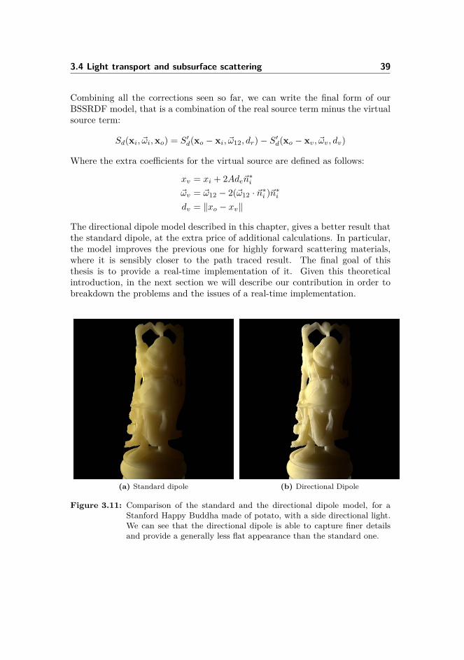
The directional dipole model described in this chapter, gives a better result thatthe standard dipole, at the extra price of additional calculations. In particular,the model improves the previous one for highly forward scattering materials,where it is sensibly closer to the path traced result. The final goal of thisthesis is to provide a real-time implementation of it. Given this theoreticalintroduction, in the next section we will describe our contribution in order tobreakdown the problems and the issues of a real-time implementation.

(a) Standard dipole (b) Directional Dipole

Figure 3.11: Comparison of the standard and the directional dipole model, for aStanford Happy Buddha made of potato, with a side directional light.We can see that the directional dipole is able to capture finer detailsand provide a generally less flat appearance than the standard one.

40 Theory

Chapter 4

Method

In this chapter, after giving the theoretical foundations in Chapter 3, we intro-duce our method to render translucent materials efficiently using the directionaldipole model. This chapter connects the theory with the implementation inChapter 5. First of all, we will give a theoretical justification of our method,deriving a discretization of the rendering equation that can be actually solvedand implemented in a GPU environment. Then, we will discuss some possiblesampling patterns and how they could possibly improve the results of the finalrendering. Then, we will introduce some details on the acquisition of scatteringparameters in an experimental environment. Finally, we will describe a methodto approximate environment lighting using an arbitrary number of directionalsources.

4.1 Method overview

First of all, we recall the general form of the rendering equation for participatingmedia using a BSSRDF (equation 3.4):

Lo(xo, ~ωo) = Le(xo, ~ωo) +∫A

∫2πS(xi, ~ωi,xo, ~ωo)Li(xi, ~ωi)V (xi)(~ni · ~ωi)d~ωidAi

42 Method

In the usual approach to offline path traced rendering, we need to integratethe radiance from all the possible sources on the surface point seen by eachpixel of the final image. For this surface element subtended by one pixel, allthe incoming radiance contributions from the other points in the scene mustbe accounted an then multiplied by the BSSRDF function in the direction ofthe camera. In a way, we are basically performing the integral in equation 3.4numerically. If we use a BSSRDF function, the contribution from all the pointsfrom the other surfaces must be employed, while in the case of a BRDF somecontributions may be excluded. Given its natural exponential explosion, pathtracing is not generally suitable for real-time rendering.

Figure 4.1: Simulation of the directional dipole BSSRDF of a laser hitting a slab of2x2 cm of potato material. We note the exponential decay of subsurfacescattering phenomena.

In our method, in its final goal to be real time, we perform the same integralas equation 3.4, but under some assumptions and restrictions that allow usto perform it more efficiently. In addition, since our method approximates theintegral and not the BSSRDF function, it is applicable to any BSSRDF function,given that it has limited or no dependence on the outgoing direction ~ωo, like the

4.1 Method overview 43

Figure 4.2: Setup for our method: the disk is placed on the point xo, displaced alongthe disc direction ~ωd and then the sample points di are reprojected backto find the samples xi.

directional dipole model.

The idea on approximating the integral comes from the fact that the directionaldipole magnitude (and subsurface scattering effects) decays exponentially fromthe point of incidence, as we can see from figure 4.1. So, the subsurface scatter-ing contribution for points that are far apart becomes quickly negligible. Thedistance to which this happens is related to the transmission coefficient σtr. Wewill investigate this relation better in the result section.

So, given this exponential decay, we place a disc on the surface for a position xo.We define a sampling disc as a point xd, a radius rd and a direction ~ωd Fromthis disc, we chose a subset of points, that are then projected on the surfaceand used to calculate the BSSRDF contribution. This set of points xi is calledsample points. To obtain a sample point from a disc point di, we take the pointthat intersects the surface along the line with direction ~ωd passing from thepoint di (see figure 4.2 for an illustration of the process). In formulas, we do:

xi = di − s~ωd, s ∈ R,xi ∈M

We note that we can have multiple s solving this equation, or none at all. If atleast one s exists, we take the one that makes the distance between di and xithe smallest. Then, we calculate and average the BSSRDF contribution fromthese points xi on the point xo. The process can be repeated more times formultiple lights, using the same set of sampling points.

44 Method

(a) Bottom sample, naıve approach (b) Side sample, naıve approach

Figure 4.3: Counter examples of the naıve choice for xd and ~ωd. The green arearepresent the sampling area of the disc (see from the side). The redarea shows where on the surface the contribution is higher for the pointxo. We can see that with this approach all the contribution is actuallymissed.

Given this setup, we need to find a way of efficiently placing the disc in orderto get a good approximation of the BSSRDF. In fact, if the disc is placed in thewrong position, the accounted contribution from the sampling points will notbe correct. Moreover, also the orientation of the disc is important, in order tonot undersample light in certain regions of the model. A naıve approach wouldsuggest to pick xd = xo and ~ωd = ~no, but we can see that this approach is notcorrect. The most obvious counter examples are displayed in Figure 4.3: in thefirst example 4.3a, the contribution from the surrounding points will be zero,because none of the sampling points is directly illuminated by the light, so thevisibility term on the rendering equation will evaluate to zero. In the secondexample (figure 4.3b), the wrong direction ~no prevents the most of the pointsfrom being sampled. A more careful choice for placing the points in the disc isto place the disc in a way that the obtained surface point is always the closestone to the light. To ensure that the points xi always have this property, we canplace xd far enough from the surface in a way that all the sampling points haveto be the closest to the light. If we define a bounding box vector in the samecoordinate frames, we have a simple formulation for xd:

xd = xo + (b · ~ωl)~ωl

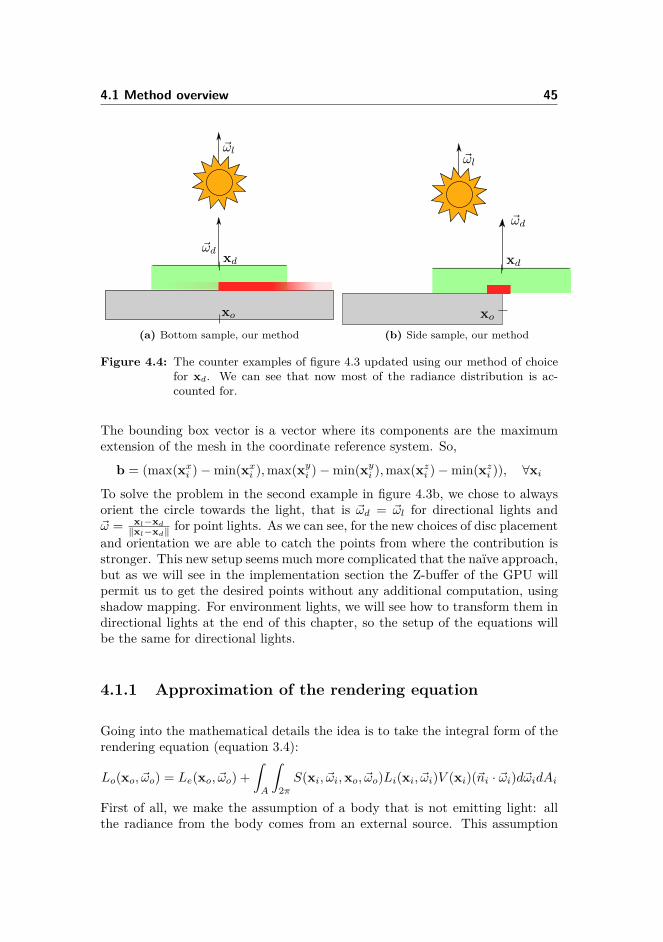
4.1 Method overview 45

(a) Bottom sample, our method (b) Side sample, our method

Figure 4.4: The counter examples of figure 4.3 updated using our method of choicefor xd. We can see that now most of the radiance distribution is ac-counted for.

The bounding box vector is a vector where its components are the maximumextension of the mesh in the coordinate reference system. So,

b = (max(xxi )−min(xxi ),max(xyi )−min(xyi ),max(xzi )−min(xzi )), ∀xiTo solve the problem in the second example in figure 4.3b, we chose to alwaysorient the circle towards the light, that is ~ωd = ~ωl for directional lights and~ω = xl−xd

‖xl−xd‖ for point lights. As we can see, for the new choices of disc placementand orientation we are able to catch the points from where the contribution isstronger. This new setup seems much more complicated that the naıve approach,but as we will see in the implementation section the Z-buffer of the GPU willpermit us to get the desired points without any additional computation, usingshadow mapping. For environment lights, we will see how to transform them indirectional lights at the end of this chapter, so the setup of the equations willbe the same for directional lights.

4.1.1 Approximation of the rendering equation

Going into the mathematical details the idea is to take the integral form of therendering equation (equation 3.4):

Lo(xo, ~ωo) = Le(xo, ~ωo) +∫A

∫2πS(xi, ~ωi,xo, ~ωo)Li(xi, ~ωi)V (xi)(~ni · ~ωi)d~ωidAi

First of all, we make the assumption of a body that is not emitting light: allthe radiance from the body comes from an external source. This assumption

46 Method

can be trivially relaxed and implemented, but to simplify the equation in thischapter we will exclude it from the calculations. Secondly, we limit ourselvesto the case of one directional light, treating the case of a point light later as anextension. The directional light direction ~ωl and radiance Ld δ(~ωd).

Under the first assumption, equation 3.4 becomes:

LDo (xo, ~ωo) =∫A

∫2πS(xi, ~ωi,xo, ~ωo)Ld δ(~ωl) V (xi)(~ni · ~ωi)d~ωidAi

LDo (xo, ~ωo) =∫A

S(xi, ~ωl,xo, ~ωo)LdV (xi)(~ni · ~ωl)dAi

In this way, we remove the internal integral. Then, we need to discretize theremaining integral. We imagine to have a set of N points on the surface. Weassume that each one of these points is visible from the light source (so we canget rid of the V (xi) term). We will discuss in the implementation section howto make sure that all these points are visible. Each one of these points has anassociated area Ai, so that we can write:

LDo (xo, ~ωo) = Ld

N∑i=1

S(xi, ~ωl,xo, ~ωo)(~ni · ~ωl)Ai (4.1)

Now, instead of using all the points on the surface, we consider only the pointswithin a certain radius r∗ from the point xo, i.e. the disk we discussed in Section4.1. Assuming the points are distributed uniformly on the disk, we obtain thefollowing area for a point:

Ai = AcN (~ni · ~ωl)

Where Ac = π(r∗)2 is the area of the circle. The ~ni · ~ωl accounts for the factthat the area is projected on the surface. Inserting into equation 4.1, we obtain:

LDo (xo, ~ωo) = LdAcN

N∑i=1

S(xi, ~ωl,xo, ~ωo) (4.2)

That is our final approximation for a directional light. For a point light, follow-ing the exact same steps, we reach a similar solution. We recall that a pointlight is defined by an intensity Ip and a source point xp:

LPo (xo, ~ωo) = IpAcN

N∑i=1

S(xi, xp−xi‖xp−xi‖ ,xo, ~ωo)‖xp − xi‖2

(4.3)

And, since the radiance is linearly summable, we can combine the contributionfrom an arbitrary number of P1, P2...Pp point sources and D1, D2...Dd direc-

4.2 Sampling patterns 47

tional sources:

Lo(xo, ~ωo) =

=p∑k=1

LPko (xo, ~ωo) +d∑k=1

LDko (xo, ~ωo)

= AcN

p∑k=1

Ikp

N∑i=1

S(xi,xkp−xi‖xkp−xi‖ ,xo, ~ωo)‖xkp − xi‖2

+d∑k=1

Lkd

N∑i=1

S(xi, ~ωkl ,xo, ~ωo)

(4.4)

4.2 Sampling patterns

As we discussed, the BSSRDF function for the directional dipole is dominated byan exponential decay. So, it is more probable to find points that contribute moreto the BSSRDF if we take points closer to the evaluation point xo. However,our assumption of uniform areas in the previous calculations does not holdanymore, so we need to modify the previous equations in order to account forthe non-linear sampling.

Assuming to have number generator that can generate numbers on a disc, wecan create an exponentially distributed disc with the following exponential prob-ability distribution function (PDF):

pdf(x) = σtre−σtrx

The difference between a disc sampled using this distribution and an uniformone is shown in figure 4.5. The process to create this distribution using rejectionsampling will be illustrated in the implementation section. We take the radiusof a point xi as ri = ‖di‖. So now we have a new normalization term to includein order to scale back the result. So, we need now to divide by a exp(−σtrri)term each sample. The new equation for a directional light instead of 4.2 thenbecomes:

LDo (xo, ~ωo) = LdAcN

N∑i=1

S(xi, ~ωl,xo, ~ωo)eσtrri

The other two equations 4.3 and 4.4 then change accordingly:

LPo (xo, ~ωo) = IpAcN

N∑i=1

S(xi, xp−xi‖xp−xi‖ ,xo, ~ωo)‖xp − xi‖2

eσtrri

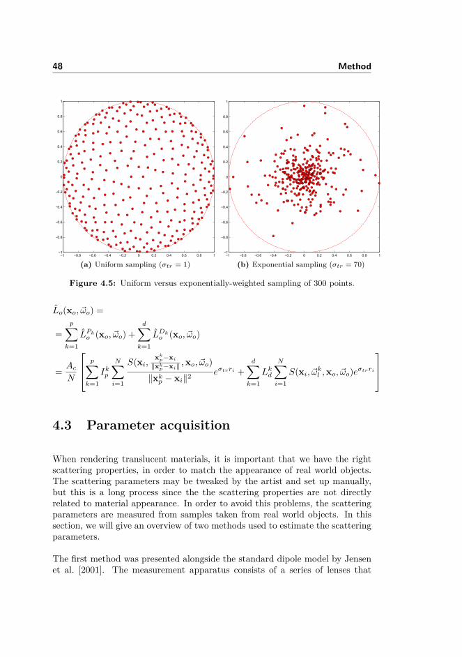
48 Method

−1 −0.8 −0.6 −0.4 −0.2 0 0.2 0.4 0.6 0.8 1−1

−0.8

−0.6

−0.4

−0.2

0

0.2

0.4

0.6

0.8

1

(a) Uniform sampling (σtr = 1)−1 −0.8 −0.6 −0.4 −0.2 0 0.2 0.4 0.6 0.8 1−1

−0.8

−0.6

−0.4

−0.2

0

0.2

0.4

0.6

0.8

1

(b) Exponential sampling (σtr = 70)

Figure 4.5: Uniform versus exponentially-weighted sampling of 300 points.

Lo(xo, ~ωo) =

=p∑k=1

LPko (xo, ~ωo) +d∑k=1

LDko (xo, ~ωo)

= AcN

p∑k=1

Ikp

N∑i=1

S(xi,xkp−xi‖xkp−xi‖ ,xo, ~ωo)‖xkp − xi‖2

eσtrri +d∑k=1

Lkd

N∑i=1

S(xi, ~ωkl ,xo, ~ωo)eσtrri

4.3 Parameter acquisition

When rendering translucent materials, it is important that we have the rightscattering properties, in order to match the appearance of real world objects.The scattering parameters may be tweaked by the artist and set up manually,but this is a long process since the the scattering properties are not directlyrelated to material appearance. In order to avoid this problems, the scatteringparameters are measured from samples taken from real world objects. In thissection, we will give an overview of two methods used to estimate the scatteringparameters.

The first method was presented alongside the standard dipole model by Jensenet al. [2001]. The measurement apparatus consists of a series of lenses that

4.3 Parameter acquisition 49

focus the light on the sample. The light power Φ is measured by calibratingthe sensor with a spectralon sample. A picture of the sample is then acquiredat different exposure, in order to build an high dynamic range image. This isnecessary since the scattering decays exponentially, so a high range is needed tohave meaningful measurements. The measured data are then fitted to diffusiontheory in order to obtain the scattering coefficients. Due to the nature of themeasurement, it is not possible to measure the mean cosine g of the material,but only the reduced scattering coefficient σ′s = σs(1 − g) and the absorptioncoefficient σa. This measurement model uses the diffusion approximation towork, so it shares the same limitations: it is valid only for materials whereσa � σs, or highly scattering materials.

The second method, proposed by Narasimhan et al. [2006] proposes a methodto measure the scattering coefficients by dilution. The assumption is that waterdoes not interfere with the scattering properties of the materials dissolved withinit for small distances (less than 50 cm). Naturally, the material needs then to bealready in a liquid form, or to be a powder that can be easily dissolved in water.The setup of the experiment is a box full of water with a camera and an arealight. High dynamic range picture of the material dissolved in water are thentaken, and the scattering coefficients can be measured analyzing the resultingimages. Various measurements at different concentrations are needed in orderto get an effective measurement of the coefficients, but then the coefficients canbe extrapolated for any concentration.

Some of the scattering properties measured thanks to this method are reportedin table 4.1. This coefficients will be used throughout the report when referenc-ing to a specific material.

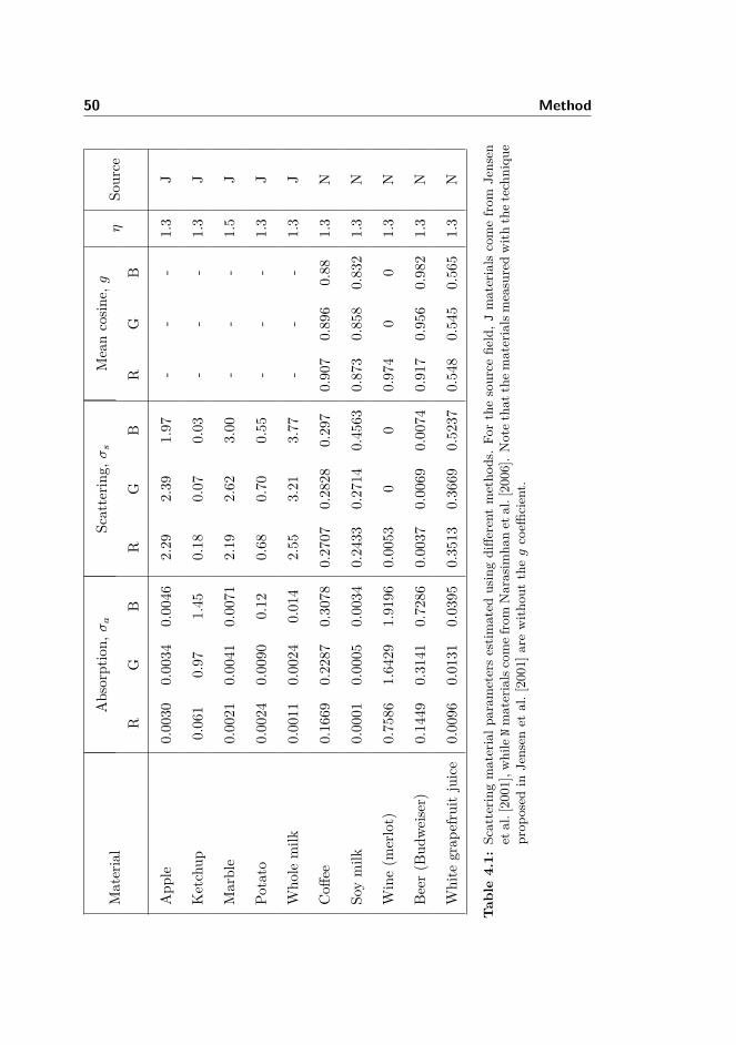
50 MethodM

ater

ial

Abs

orpt

ion,σa

Scat

terin

g,σs

Mea

nco

sine,g

ηSo

urce

RG

BR

GB

RG

B

App

le0.

0030

0.00

340.

0046

2.29

2.39

1.97

--

-1.

3J

Ket

chup

0.06

10.

971.

450.

180.

070.

03-

--

1.3

J

Mar

ble

0.00

210.

0041

0.00

712.

192.

623.

00-

--

1.5

J

Pota

to0.

0024

0.00

900.

120.

680.

700.

55-

--

1.3

J

Who

lem

ilk0.

0011

0.00

240.

014

2.55

3.21

3.77

--

-1.

3J

Coff

ee0.

1669

0.22

870.

3078

0.27

070.

2828

0.29

70.

907

0.89

60.

881.

3N

Soy

milk

0.00

010.

0005

0.00

340.

2433

0.27

140.

4563

0.87

30.

858

0.83

21.

3N

Win

e(m

erlo

t)0.

7586

1.64

291.

9196

0.00

530

00.

974

00

1.3

N

Beer

(Bud

weise

r)0.

1449

0.31

410.

7286

0.00

370.

0069

0.00

740.

917

0.95

60.

982

1.3

N

Whi

tegr

apef

ruit

juic

e0.

0096

0.01

310.

0395

0.35

130.

3669

0.52

370.

548

0.54

50.

565

1.3

N

Tab

le4.

1:Sc

atte

ring

mat

eria

lpar

amet

ers

estim

ated

usin

gdi

ffere

ntm

etho

ds.

For

the

sour

cefie

ld,J

mat

eria

lsco

me

from

Jens

enet

al.[

2001

],w

hile

Nm

ater

ials

com

efr

omN

aras

imha

net

al.[

2006

].N

ote

that

the

mat

eria

lsm

easu

red

with

the

tech

niqu

epr

opos

edin

Jens

enet

al.[

2001

]are

with

out

theg

coeffi

cien

t.

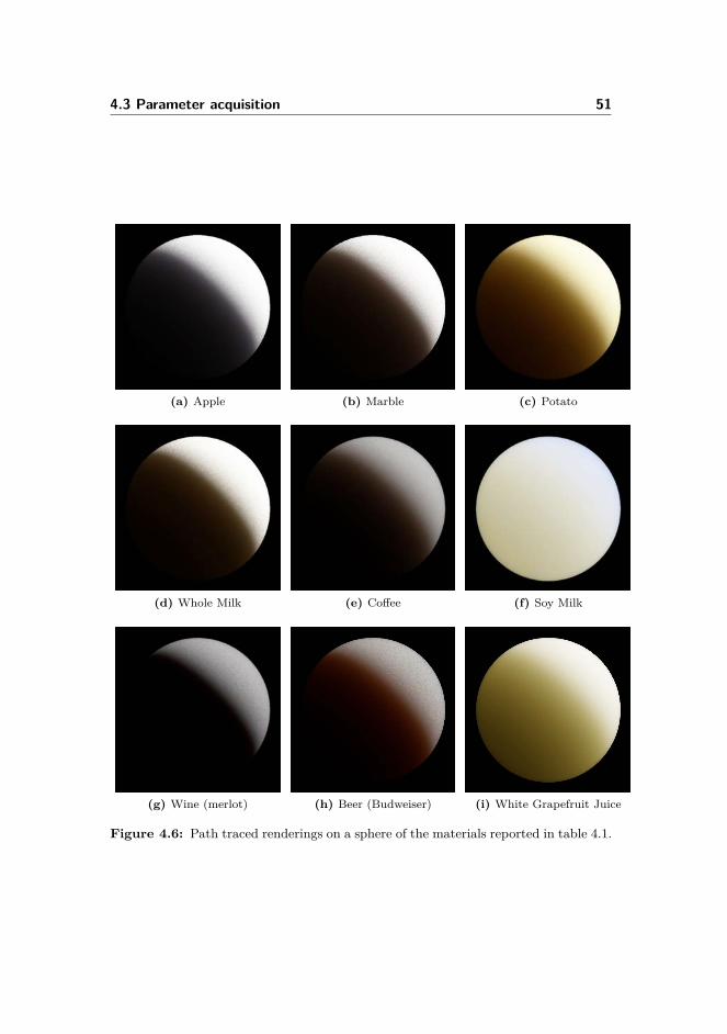
4.3 Parameter acquisition 51

(a) Apple (b) Marble (c) Potato

(d) Whole Milk (e) Coffee (f) Soy Milk

(g) Wine (merlot) (h) Beer (Budweiser) (i) White Grapefruit Juice

Figure 4.6: Path traced renderings on a sphere of the materials reported in table 4.1.

52 Method

4.4 Environment lights

Environment lighting is a omni-directional type of lighting that represents lightcoming from an environment. Instead of defining a light as a direction or apoint in space, we define directly the radiance distribution on a map. The mapis usually provided in a HDR format in order to cover various range of radiancevalues, and it is usually given as a set of six cube faces (cubemap) or as alatitude-longitude map, as the one in Figure 4.7. The maps are usually given inequirectangular projection.

In the game development community, spherical harmonics (SH) [Green, 2003,Sloan, 2008] are usually employed. This technique, given an heavy pre-computationstep, transforms the radiance map into a set of coefficients in the spherical har-monics basis. This coefficients can be used easily to represent the low frequencycomponent of the radiance map Ramamoorthi and Hanrahan [2001].

Figure 4.7: Latitude - longitude environment map of the inner courtyard of theDoge’s palace in Venice (Doge map). The map has been convertedto a RGB format from the original HDR format. This and all themaps used in this report are courtesy of http://gl.ict.usc.edu/Data/HighResProbes/.

In this chapter, we introduce a technique presented in Pharr and Humphreys[2004] to convert a environment map into a set of directional light sources ofarbitrary size. The general idea is to generate a set of random points and themtransform them according to a pre-computed probability distribution. Thisdistribution make the random point concentrate in areas where the radiance ishigher, so that it is possible to get the most representative points on the radiance

4.4 Environment lights 53

map. The found points are then transformed into a spherical coordinate basisin order to get the light direction.

We start defining our image as an array of n rows and m columns. We needto define a function that of each pixel of the image gives us a single radiancevalue. Instead of using radiance, we use luminance. The ITU-R recommenda-tion standard BT.709 [ITU, 2001] gives us a formula to obtain luminance fromspectral radiance values:

f(u, v) = 0.2126 R(u, v) + 0.7152 G(u, v) + 0.0722 B(u, v)

Where [u, v] ∈ [0, n) × [0,m). R, G and B represent the spectral coordinatesof the radiance map. We would like to define now a probability distributionfunction based on the f(u, v) function. We can define it simply by normalizingf with the integral of the function over the domain:

p(u, v) = f(u, v)∫∫f(u, v)dudv

= f(u, v)∑u

∑v

f(u, v)

However, in order to be able to sample from the distribution p(u, v), there aresome things to take care about. We would like now to separate the two variables,in order to sample from two one-dimensional distributions, instead of one two-dimensional distribution. To do this, we use the conditional probability formula:

p(u, v) = pv(v|u)pu(u) (4.5)

So that we first choose u, sample its probability pu(u) and then compute theconditional density pv(v|u) using the found value for u. Using the marginalformulas, the first probability is easily found:

pu(u) =∫p(u, v)dv =

∑v

f(u, v)∑u

∑v

f(u, v)

And, from equation 4.5, we find the conditional probability:

pv(v|u) = p(u, v)pu(u) = f(u, v)∑

v

f(u, v)sin θ

The sin θ comes from the fact that the latitude-longitude map with a equirectan-gular projection is not area preserving. So, the sampling must take into accountthe distortion of the map, otherwise the samples will be more concentrated atthe poles, rather than distributed uniformly on the sphere. We can appreciate

54 Method

−1

−0.5

0

0.5

1

−1

−0.5

0

0.5

1

−1

−0.8

−0.6

−0.4

−0.2

0

0.2

0.4

0.6

0.8

1

(a) Without sin θ correction−1

−0.5

0

0.5

1

−1

−0.5

0

0.5

1

−1

−0.8

−0.6

−0.4

−0.2

0

0.2

0.4

0.6

0.8

1

(b) With sin θ correction

Figure 4.8: Effect of sin θ on a random point distribution on a sphere.

the difference for a random sampling on a sphere in Figure 4.8. Now we are readyto sample the function. In order to bias our sample according to the radiancedistribution, we need to calculate the cumulative distribution function (CDF)for a one-dimensional probability distribution function, then inverse sample it.The CDF is defined as:

cu(u) =∫ u

−∞pu(u)du =

u∑i=0

pu(u)

That is the discrete integral of the function up to the point u. Figure 4.9 explainswhy we need to inverse sample the CDF. If, as the figure, all the radiance isdistributed towards the right side of the picture (i.e. the CDF rises slowly), ifwe pick a set of random points (on the y axis) and inverse sample the CDFon them (on the x axis), we obtain a new set of points that is biased towardsthe highest concentration of radiance. Let us now pick a couple of randompoints (ζ1, ζ2) ∈ [0, 1)2. We then convert these points to a pair of coordinates(u1, u2) ∈ [0, n)× [0,m) by inverse sampling of the CDF. We will give the detailsof how to discretize this process in the implementation section. Then, we obtainthe spherical coordinates using the standard formula:

(θ, φ) =( u1

πn,u2

2πm

)And, from the spherical coordinates, we use the equirectangular projection for-mula to transform them into a vector in the 3D space, that is the final direction

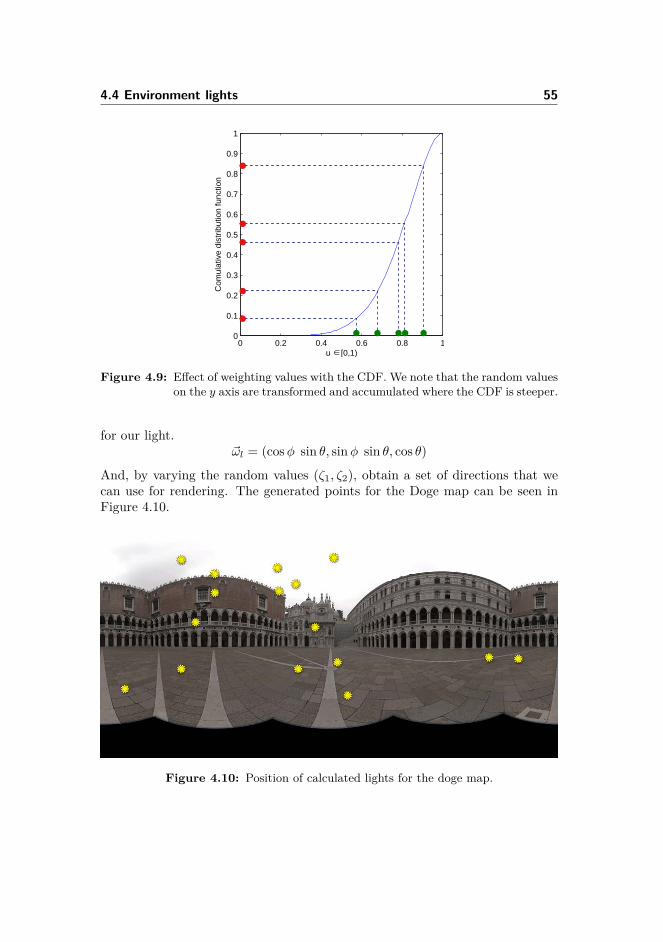
4.4 Environment lights 55

0 0.2 0.4 0.6 0.8 10

0.1

0.2

0.3

0.4

0.5

0.6

0.7

0.8

0.9

1

uc∈[0,1)

Com

ulat

ivec

dist

ribut

ionc

func

tion

Figure 4.9: Effect of weighting values with the CDF. We note that the random valueson the y axis are transformed and accumulated where the CDF is steeper.

for our light.~ωl = (cosφ sin θ, sinφ sin θ, cos θ)

And, by varying the random values (ζ1, ζ2), obtain a set of directions that wecan use for rendering. The generated points for the Doge map can be seen inFigure 4.10.

Figure 4.10: Position of calculated lights for the doge map.

56 Method

Chapter 5

Implementation

In this chapter, we will introduce the implementation of our method. We willfocus on a GPU-oriented implementation of the method presented in Chapter4. First, we will briefly introduce the environment in which we are operating.Then, we will give a general outline of our algorithm. Then, we will discuss inmore detail some of the ideas introduced in the outline. After this discussion,we will discuss some defects and artifacts in our algorithm that arose duringthe implementation, and how we have solved them. Finally, we will extendour implementation to different kind of lights. Finally, we will discuss ourimplementation.

5.1 Environment

In order to justify some of the choices and the code parts that will be introducedin this section, we will first introduce the environment of our implementation.The method we are going to discuss was made using the OpenGL API, version4.3 (released in August 2012), a multi-platform API used for rendering 2D and3D accelerated graphics. With the OpenGL API comes GLSL, the OpenGLShading Language, used for writing pieces of code to be run on the GPU, calledshaders. Our method uses some advanced features of OpenGL 4.3, so it is not

58 Implementation

immediately portable to previous generation hardware, and runs only on high-end modern GPUs. On the CPU side, we use an extended framework basedon Qt, a C++ library that allows to create a OpenGL context and graphicalinterfaces in an easy way.

5.2 Algorithm overview

By keeping the limitations presented in Chapter 1 in mind, we introduce ouralgorithm. The algorithm is inspired by translucent shadow maps [Dachsbacherand Stamminger, 2003], that we presented in Chapter 2. The general ideais to first render the scene from the light point of view, then place the diskwe discussed in the previous Chapter (Section 4.1) directly on the generatedtexture, storing the result in a radiance map. We use many directions in orderto capture all the sides of the object. Finally, we sample from the obtainedradiance map for the final rendering.

In this section, we will assume to only have one directional light with radianceLd and direction ~ωd, with one not-deformable object in the scene. We willdiscuss later how to extend the method to multiple light sources.

Step 1 - Light bufferIn the first step, positions and normals of the object are rendered into a texturefrom the light point of view. We will refer to the resulting texture as thelight map. As in standard shadow mapping we create and store a matrix toconvert between world space and texture light space. Depth testing in thisstep is enabled. More details on the implementation of a render to texture arepresented in Section 5.3.1.

5.2 Algorithm overview 59

Figure 5.1: Render to G-buffer. Note that the frustum and the light direction arealigned.

(a) Vertex buffer (b) Normal buffer

Figure 5.2: State of the vertex and normal buffer after rendering from a directionallight. The model used was the Stanford bunny from the Standford 3DScanning repository.

60 Implementation

Step 2 - Render to radiance mapIn the second step, we render the object from K different directions into anothertexture, called the radiance map. The radiance map is organized as a layeredtexture, where each layer represents a direction. More details on render totexture and layered textures are presented in sections 5.3.1 and 5.3.2. Thepoints on which to place the cameras are chosen randomly, distributed on asphere (see Section 5.3.4 for the details). The cameras point towards the centerof the object bounding box.

On this step, for each pixel that corresponds to an exiting point xo the shadersamples N points from the texture rendered in the previous step. If the sampledpoint is valid, it is then used to calculate the BSSRDF and accumulate it in theresulting radiance map. So, this step calculates the following:

Rk(xo) = Ld

N∑i=1

S(xki , ~ωl,xo, ~ωo) exp(σtrr

ki

), k ∈ [0,K − 1] (5.1)

Where we recall that we have introduced an exponential term in order to com-pensate for the exponential displacement of the sampling pattern. The genera-tion of the sampling pattern is described in Section 5.3.4.1 in more detail. Weintroduced a k parameter, that represents the current direction we are renderingto. We can see how we are rendering a point from one of the considered direc-tions in Figure 5.4. Also in this case, the texture space - world space conversionmatrices are stored and prepared to be reused in step 3, where we will combinethe results.

We can appreciate that rendering the light from the camera point of view comeswith two important advantages:

• If the disk is placed in texture space, it is automatically oriented towardsthe light direction, that is ~ωd = ~ωl.

• The light renders in the texture only the points directly visible from it,that are also the only points directly lit. In addition, if we sample thelight map on any point, we get the corresponding vertex that is closest tothe light.

This two factors allows us to sample the most optimal point and direction inwhere to place the disk, as we described it in Section 4.1.

5.2 Algorithm overview 61

Figure 5.3: Render to the radiance map. When we render the point xo, the posi-tion in the light map is calculated and the values xi in the samples arecalculated and summed over.

In addition, on each layer, we accumulate the result over different frames:

Rt,k =t−1∑i=0

Ri,k +Rt,k = Rt−1,k +Rt,k

R here represents the value that is stored in the radiance map. In equation5.1, we omitted the dependence from time for the sake of clarity. We need anaccumulation process in order to deal with the fact that the result from theprevious computation are not reaching a satisfying result within one frame, sothey need to be accumulated over a period of T frames in order to reach anappreciable result. In order to do this, the sampled points need to change ondifferent frames (in Section 5.3.4 we give more details on the process).

Naturally, the accumulation process works only if the scene does not change. Achange can be a relative change of positions between the points on the modeland the light, so if the model gets translated, rotated or scaled, the accumulated

62 Implementation

x

Figure 5.4: Render to cubemap, side view. The gray area represents the frustum ofthe current direction’s camera (orthographic). We have three differentcases of a point on the surface: x1

o is visible from both the light and thecamera, so the disk is placed on it. x2

o is visible from the camera but notfrom the light, so the disk is placed in the closest position to the light.x3o is not visible from the camera, so it is discarded.

result has to be discarded and the accumulation started all over. The directionalcameras are locked with the model, so the pixels are always aligned. This iswhy in equation 5.1 the dependence from time of the point xo and ~ωo have beendropped.

Step 3 - CombinationIn this step, we render our model. Using the matrices and the textures preparedin the previous step, for each fragment on the surface we sample all the layersin the texture as illustrated in Figure 5.5. In order to do this, we need alsoto sample the depth map generated in the previous step. We can define thissampling as a visibility function to test if a point x belongs to layer k:

V k(x) ={

1 if x is visible from the kth camera0 otherwise

The function V is calculated by sampling the k-th layer depth map in a way

5.2 Algorithm overview 63

similar to shadow mapping (details in Section 5.3.5). Given this function, wecan simply represent the outgoing radiance by simply averaging the summationover the K layers:

LtSS(x) = AcNt

K−1∑k=0

V k(x)Rt,k(x)

K−1∑k=0

V k(x)

The first factor 1t is to average over the number of frames, while the second is the

average area of a sample in the circle AcN , that is necessary to complete equation

4.2. We note that we moved all the layer-independent computation into thefinal computation step, in order to save as much performance as possible.

Figure 5.5: Final combination step. The blue quads indicates each one of the radi-ance map layers, as seen from their direction. We can see that in thepoint xo the contribution from three faces (green dots) is considered. Forthe remaining two faces (red dots), the contribution is not considered asthe point is not visible.

We are not done yet, as for now we have computed the radiance only derivingfrom subsurface scattering. For finally describing the illumination of our scene,we need also to include a factor based on the surface reflection. Since thesubsurface scattering radiance is already multiplied by a transmittance Fresnel

64 Implementation

term (in the BSSRDF equation in 3.9) T (η, ~ωo) we the reflection color multipliedby the converse transmission term 1− T (η, ~ωo):

Lt(x, ~ωo) = LtSS(x) + (1− T (η, ~ωo))Li(x, ~ωo − 2(~ωo · ~n)~n)

Li can be the radiance coming from other objects or by an environment map.After this, we just need to perform gamma correction in order to get the finalresult. Given the gamma coefficient γ, we perform gamma correction by:

Ltgamma(x, ~ωo, γ) = Lt(x, ~ωo)1γ

And, adter this, we can finally send the radiance to the output device.

Figure 5.6: Final Result of the method after 100 frames simulating a potato bunny ofdimensions ≈ 30cm. All the results presented in this report are gammacorrected with γ = 1.8.

5.3 Implementation details 65

Figure 5.7: Final Result of the method after 100 frames simulating a backlit bunnymade of beer, dimensions ≈ 30cm.

5.3 Implementation details

In this section, we will further expand the overview given in the previous sectionby adding further details. We organized this section in topics, in each one ofthem expanding a particular aspect of our algorithm. Each point clarifies withexamples one technique or approach used in the method. The code given oneach example does not necessarily come from our implementation, but it can besimplified for illustration purposes.

5.3.1 Render-to-texture

In a graphics API, and more specifically in OpenGL, all the output from a finalshader stage is usually sent to the display device in order to be displayed on

66 Implementation

the screen. However, it is possible to redirect the output into another memoryarea of the GPU and reuse it for further computations. This allows to createcomplicated rendering techniques such as the one described in this report.

In OpenGL, is possible to redirect the output to a texture object. We can do thisthrough a so-called framebuffer object (FBO). A FBO is a collection of objectsthat allows off-screen rendering. A FBO has attachment points, to which we canattach textures. A texture can be attached to one of the output color channels ofthe fragment shader (GL_COLOR_ATTACHMENT0, GL_COLOR_ATTACHMENT1, ...), tothe depth buffer output (GL_DEPTH_ATTACHMENT) or to the stencil buffer output(GL_STENCIL_ATTACHMENT).

The connection between the framebuffer and the texture can be set in a ini-tialization step (listing 5.1). Then, by simply binding the FBO (listing 5.2) weredirect our screen output to the desired texture.

GLuint tex ,fbo;// Generating textureglGenTextures (1, &tex);glBindTexture ( GL_TEXTURE_2D , tex);[...] // setting up texture parameters ...glTexImage2D ( GL_TEXTURE_2D , 0, GL_RGBA16F , size , size , 0, GL_RGBA , GL_FLOAT←↩

, 0);

glGenFramebuffers (1 ,& fbo);

// connecting current fbo and textureglBindFramebuffer ( GL_DRAW_FRAMEBUFFER , fbo);glFramebufferTexture2D ( GL_DRAW_FRAMEBUFFER , GL_COLOR_ATTACHMENT0 , ←↩

GL_TEXTURE_2D , tex , 0);glBindFramebuffer ( GL_DRAW_FRAMEBUFFER , 0); // Binding back main framebuffer

Listing 5.1: Render to texture example, initilalization phase. Note the call toglFramebufferTexture2D

glBindFramebuffer ( GL_DRAW_FRAMEBUFFER , fbo);GLenum buffers [] = { GL_COLOR_ATTACHMENT0 };glDrawBuffers (1, buffers );[...] // draw model

Listing 5.2: Render to texture example, rendering phase. Since we have notconfigured and FBO for depth and stencil buffers, depth testing andstencil should be disabled at this point.

5.3 Implementation details 67

5.3.2 Layered rendering

Layered rendering is a special feature used to render to a special type of texturecalled layered texture. Let us take as an example the step 2 of our algorithm,where we need to render the object from K different directions. A first approachto this would be to create K 2D textures of type GL_TEXTURE_2D, and performK draw calls, rebinding the texture on the current FBO each time. OpenGL,however, provides a way to do this with a single draw call, potentially reducingthe rendering costs due to context switching.

We will use the OpenGL provided type GL_TEXTURE_2D_ARRAY, that we initializein the usual way, noting that an array texture should be allocated as a 3D tex-ture. When binding it to an FBO, we use the generic glBindFramebufferTexture:

GLuint fbo , arraytex ;glGenFramebuffers (1 ,& fbo);glGenTextures (1, & arraytex );

glBindTexture ( GL_TEXTURE_2D_ARRAY , arraytex );[...] // setting up texture parameters , omittedglTexStorage3D ( GL_TEXTURE_2D_ARRAY , levels , GL_RGBA32F , size , size , layers );

glBindFramebuffer ( GL_DRAW_FRAMEBUFFER , fbo);glFramebufferTexture ( GL_DRAW_FRAMEBUFFER , GL_COLOR_ATTACHMENT0 , arraytex , ←↩

0);

Listing 5.3: Initializing array texture. Note that the number of layers is passed tothe glTexStorage3D command.

In order to render to a layered texture, we need then to introduce a geometryshader. In our example, the difference between each layer is basically a differentview matrix. So, we move the computation of the position, usually left to thevertex shader, to the geometry shader. We first introduce the code:

#version 430#define DIRECTIONS 16layout ( triangles ) in;layout ( triangle_strip , max_vertices = 60) out;

uniform mat4 P;uniform mat4 viewMatrices [ DIRECTIONS ];

void main(void){

for(int i = 0; i < DIRECTIONS ; i++){

gl_Layer = i;

for(int k = 0; k < 3; k++){

vec4 v = gl_in [k]. gl_Position ;

68 Implementation

gl_Position = P * viewMatrices [i] * v;EmitVertex ();

}EndPrimitive ();

}}

Listing 5.4: Geometry shader for layered rendering. The multiplication by the modelmatrix of vertex v is performed in the vertex shader (not shown).

VERTEX SHADER VERTEX SHADER VERTEX SHADER

GEOMETRY SHADER

FRAGMENT SHADER FRAGMENT SHADER FRAGMENT SHADER FRAGMENT SHADER

LAYERED TEXTURE

Figure 5.8: Diagram that illustrates layered rendering.

5.3 Implementation details 69

As we can see, we duplicate each one of the incoming triangles and then outputit multiplied by a different view matrix. the EndPrimitive() function ensuresthat the output triangles in the final triangle strip are separated. In order torender each triangle to a different layer, we need to set the build-in variablegl_Layer to the layer we want to render before emitting the triangle. Thewhole process is illustrated in Figure 5.8.

5.3.3 Accumulation buffers

In the second step of our method we said we would like to accumulate the resultof the computation, in order to progressively update the result over differentframes. In order to do this, we encounter an obstacle: we would like to renderto the currently bound texture, but at the same time we need to read theprevious value stored on the texture. Unfortunately, the OpenGL Specification[Segal and Akeley, 2012] advices against reading from the same texture we arerendering to. This is made to avoid a situation called feedback loop. In fact, wecannot be sure of the results of what is stored in any pixel of the texture whilewe are rendering to it.

There are many possible solutions to the problem. The first approach is torely on the driver implementation: some drivers, in fact, allow to render to thesame texture we are bound to, under some conditions. However, if we want ageneral method that works over all platforms, this is not a viable path. Thesecond solution is to use image textures, a new type introduced in OpenGL 4.2that allows explicit load-store of values, as well as new special constructs forGPU memory management (atomic operations and memory barriers). Thoughthe usage of these features is appealing, their performance is generally poorcompared to a framebuffer-based implementation.

The final approach, and the one we use in our implementation, is to ping-pongbetween the two textures. The idea is to sacrifice memory space by employingtwo textures T1 and T2. In the first frame, we render to the first texture T1.In the second frame, we use T2 as a render target, and we sample T1 and addit to the computed result. In the third frame, we render to T1 and samplefrom T2, and so on. From this alternance between the textures comes the nameping-pong. A minimal example of ping-ponging using a 2D texture is shown inlisting 5.5.

70 Implementation

// A global frame variable is initialized in order to keep track of the ←↩current frame

GLuint fbo , tex1 , tex2;// Creating FBO , initializing textures and texture parameters .// Also binding shader with glUseProgram in order to bind texture uniforms[...]

GLuint tex_from , tex_to ;

tex_from = ( frame % 2 == 0)? tex1 : tex2;tex_to = ( frame % 2 == 0)? tex2 : tex1;

glBindFramebuffer ( GL_DRAW_FRAMEBUFFER , fbo);glFramebufferTexture ( GL_DRAW_FRAMEBUFFER , GL_COLOR_ATTACHMENT0 , tex_to , 0);glDrawBuffer ( GL_COLOR_ATTACHMENT0 );

GLint location = glGetUniformLocation (" source_texture ");glUniform1i (location , 0);glActiveTexture ( GL_TEXTURE0 );glBindTexture ( GL_TEXTURE_2D , tex_from );

// more uniforms and rendering commands .[...]frame ++;

Listing 5.5: Minimal example of ping-pong textures.

5.3.4 Generation of uniformly distributed points

In our method we have at least twice the necessity to generate uniformly dis-tributed points either on a disc or on a sphere. To do this, we employ a particularsequence of pseudo-random numbers, called Halton points [Halton, 1964]. Weexplain briefly the ideas behind the sequence. For a more mathematical com-plete discussion on its properties of pseudo randomness, see Niederreiter [1992].

First, given a prime number p and a non-negative integer n, we can express itin base p as:

n = a0 + a1p+ a2p2 + ...+ arp

r

Where ai ∈ [0, p− 1]. We now define a van der Corput sequence Φp(n) as:

Φp(n) =r∑i=0

aipi+1 = a0

p+ ...+ ar

pr

This sequence, given the fact that is based on prime points, automatically as-sumes good qualities of randomness. In addition, the function is already nor-malized in the range [0, 1). We define an Halton point as the combination oftwo Van der Corput sequences:

Hp1,p2(n) = (Φp1(n),Φp2(n))

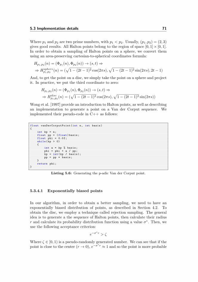
5.3 Implementation details 71

Where p1 and p2 are two prime numbers, with p1 < p2. Usually, (p1, p2) = (2, 3)gives good results. All Halton points belong to the region of space [0, 1]× [0, 1].In order to obtain a sampling of Halton points on a sphere, we convert themusing an area-preserving cartesian-to-spherical coordinates formula:

Hp1,p2(n) = (Φp1(n),Φp2(n))→ (s, t)⇒⇒ Hsphere

p1,p2(n) = (

√1− (2t− 1)2 cos(2πs),

√1− (2t− 1)2 sin(2πs), 2t− 1)

And, to get the point on a disc, we simply take the point on a sphere and projectit. In practice, we put the third coordinate to zero:

Hp1,p2(n) = (Φp1(n),Φp2(n))→ (s, t)⇒⇒ Hdisc

p1,p2(n) = (

√1− (2t− 1)2 cos(2πs),

√1− (2t− 1)2 sin(2πs))

Wong et al. [1997] provide an introduction to Halton points, as well as describingan implementation to generate a point on a Van der Corput sequence. Weimplemented their pseudo-code in C++ as follows:

float vanDerCorputPoint (int n, int basis ){

int kp = n;float pp = ( float ) basis ;float phi = 0.0f;while (kp > 0){

int a = kp % basis ;phi = phi + a / pp;kp = int(kp / basis );pp = pp * basis ;

}return phi;

}

Listing 5.6: Generating the p-adic Van der Corput point.

5.3.4.1 Exponentially biased points

In our algorithm, in order to obtain a better sampling, we need to have anexponentially biased distribution of points, as described in Section 4.2. Toobtain the disc, we employ a technique called rejection sampling. The generalidea is to generate a the sequence of Halton points, then calculate their radiusr and calculate its probability distribution function using a value σ∗. Then, weuse the following acceptance criterion:

e−σ∗r > ζ

Where ζ ∈ [0, 1) is a pseudo-randomly generated number. We can see that if thepoint is close to the center (r → 0), e−σ∗r ≈ 1 and so the point is more probable

72 Implementation

Figure 5.9: Positions of the first 16 cameras generated using Halton points on asphere.

−1 −0.8 −0.6 −0.4 −0.2 0 0.2 0.4 0.6 0.8 1−1

−0.8

−0.6

−0.4

−0.2

0

0.2

0.4

0.6

0.8

1

Figure 5.10: Exponentially biased Halton points on a disk. The maximum radius is1, and M = 300.

5.3 Implementation details 73

to be accepted. On the other hand, if the point is far from the center of the disc(r → +∞), e−σ∗r ≈ 0 and so the point is less probable to be accepted. Thecode for generating a vector of accepted points is reported in listing 5.7.

void planeHaltonCircleRejectionExponential (std :: vector <Vec2f > &result , int ←↩m, float sigma_tr , float radius )

{uint accepted = 0;

gel_srand (0); // Setting the seed of the random numberint i = 1;while ( accepted < m){

Vec2f point = haltonPointCircle (i, 2, 3);float rad = point . length () * radius ;float expon = exp(- sigma_tr * rad);float zeta = gel_rand () / (( float )( GEL_RAND_MAX ));if(zeta < expon ){

result . push_back ( radius * point );accepted ++;

}i++;

}}

Listing 5.7: Generation by rejection of a exponentially distributed disc. The functiongenerates M points with distribution e−σtrr, and where radius is themaximum final radius of the points.

In our algorithm, we generate a number of samples M that is fixed, with aradius equal to the size of the bounding box of the model. Then in the actualcalculation only theN points closest to xo are actually used, allowing us to tweakthe performance and the result. Moreover, the value of the exponent σ∗ we passto this method is related to σtr (that is a vector, since the transmission ratesare spectral), to account for the material scattering properties. We calculate σ∗with the formula:

σ∗ = min(σtr,x, σtr,y, σtr,z)q

Where q is a parameter tweakable from the user. We will justify why we usethe minimum transmission coefficient has to be used in section 6.2.1. The ideais that the user can modify the distribution of the points, making them spana wider area (that is for q > 1) without increasing the number of samples N .In fact, a bigger N implies a worse performance, while a bigger q requires onlyto recompute the points. We will discuss the results for varying values of q inChapter 6.

74 Implementation

5.3.5 Shadow mapping

Shadow mapping is a common technique used in modern real-time graphics[Everitt et al., 2003, Segal et al., 1992, Williams, 1978]. The idea behind it is torender an object from a light’s point of view, and then use the generated depthinformation in order to decide if a point is shadowed or not. First of all, weconvert the point into the light camera space, using a special space conversionmatrix. After this, if we have a point p = (px, py, pz), we compare pz to thetexture T sampled in the point (px, py):

pz > T (px, py) (5.2)

Figure 5.11: Shadow mapping. We see the different results for three points p1,p2 and p3. The red length represents the value sampled from thedepth texture(T (px, py)), while the green length represents the valuewe compare against (pz). When pz is less than T (Pxy), as in p1, thepoint is not shadowed. In the other cases, p2 and p3, pz > T (Pxy)andthe point is not visible.

5.3 Implementation details 75

If the above condition is verified, it means that the current point is beneath thepoint visible from the light and then it should be shadowed. The matrix L usedto convert a point from world space to texture space is the following, using thematrix definitions and notation in Section A:

L = T

(12

)· S(

12

)· P · V

where P and V are the projection and view matrix we use to render with thelight. The first two matrices are necessary to convert between clip and texturecoordinates, as clip coordinates are in the range [−1, 1]× [−1, 1], while texturecoordinates are in the range [0, 1] × [0, 1]. The process is illustrated in Figure5.11.

In our algorithm, we use the ideas behind shadow mapping in two differentoccasions. The first occasion is to get the points xi in step 2 from the texturegenerated in step 1, where we use the matrix L in order to convert the worldpoint xo to xd, the center of the disc in texture space.

The second occasion is in the final combination step, where we use also shadowmapping in order to compute the visibility function V k(x), and to sample theradiance map. Technically, the ”light cameras” in this case are the directionalcameras from where we render the scene, but the concept is the same. Wecan see how we sample the shadow map in the final combination shader in thefollowing listing:

#version 430uniform sampler2DArrayShadow depthMap ;uniform mat4 cameraMatrices [ DIRECTIONS ];

float sample_shadow_map (vec3 world_pos , int layer ){

vec4 light_pos = cameraMatrices [ layer ] * vec4(world_pos ,1.0f);light_pos .z -= shadow_bias ; // bias to avoid shadow acneif( light_pos .x < 0.0 || light_pos .x > 1.0) return 1.0;if( light_pos .y < 0.0 || light_pos .y > 1.0) return 1.0;return texture (depthMap ,vec4( light_pos .x, light_pos .y,layer , light_pos .z)←↩

).r;}[...] // shader code

Listing 5.8: Sampling of the shadow map texture in step 3 of our method.

In the above code, cameraMatrices[layer] corresponds to the L matrix. Weuse a special type of sampler, sampler2DArrayShadow, that makes somethingmore than its equivalent sampler2DArray. The latter, in fact, accepts a vec3,and simply retrieves the value in the texture. The former, on the other hand,accepts an extra parameter zcamera (which is light_pos.z), and compares it

76 Implementation

to the value stored in the depth texture ztex, performing the test in equation5.2. If the depth of the point is less than the depth stored in the texture(zcamera < ztex), 1 is returned as the point is closer to the directional camera,and thus visible. On the other hand, if zcamera ≥ ztex, it means the point isunder the surface, and thus not visible, and 0 is returned.

To configure the sampler2DArrayShadow texture, we need to specify some extraparameters during the depth texture initialization:

glBindTexture ( GL_TEXTURE_2D_ARRAY , depthtex );glTexParameterf ( GL_TEXTURE_2D_ARRAY , GL_TEXTURE_MIN_FILTER , GL_NEAREST );glTexParameterf ( GL_TEXTURE_2D_ARRAY , GL_TEXTURE_MAG_FILTER , GL_NEAREST );glTexParameterf ( GL_TEXTURE_2D_ARRAY , GL_TEXTURE_WRAP_S , GL_CLAMP_TO_EDGE );glTexParameterf ( GL_TEXTURE_2D_ARRAY , GL_TEXTURE_WRAP_T , GL_CLAMP_TO_EDGE );glTexParameterf ( GL_TEXTURE_2D_ARRAY , GL_TEXTURE_COMPARE_MODE , ←↩

GL_COMPARE_REF_TO_TEXTURE );glTexParameterf ( GL_TEXTURE_2D_ARRAY , GL_TEXTURE_COMPARE_FUNC , GL_LESS );glTexStorage3D ( GL_TEXTURE_2D_ARRAY , 1, GL_DEPTH_COMPONENT32F , size , size , ←↩

layers );

Listing 5.9: Configuration of a shadow map depth texture.

We can see that we specify two extra parameters: GL_TEXTURE_COMPARE_MODE,once set to GL_COMPARE_REF_TO_TEXTURE, means that sampling the depth tex-ture in a shader will give a value based on the comparison between an extra valuez and the depth value d in the texture. The second parameter GL_TEXTURE_COMPARE_FUNC specifies how to compare the values: GL_LESS means that 1 isreturned if z < d, and zero is returned otherwise.

5.3.6 Memory layout

In this section, we briefly describe how we allocate memory in our method.The great advantage of using OpenGL 4.3 is that we can use texture views[Segal and Akeley, 2012]. Texture views are a way to create allocate storagefor a texture in OpenGL, but on the opposite hand of glTexImage*D or theglTexStorage*D families of functions they allow to use another texture’s storagespace. To create a texture view, we use glTextureView. We compare thestandard way of allocating texture with our without texture view in Figure5.12.

In our method, this comes to great advantages in two areas. First of all, sincethe depth texture of the radiance map is not accumulated, we can make thetwo radiance maps that are using ping-ponging share the same depth map. Inaddition, we can render directly between two mipmap levels of the same texture,something that we will need later to generate a blurred version of our texture.

5.3 Implementation details 77

glTexStorage(...) glTexStorage(...)

texture1 texture2

(a) Without texture views

glTexStorage(...)glTextureView(...)

texture1 texture2

(b) With texture views

Figure 5.12: Diagram illustrating texture views. On the top part of the picture thetexture ids on the GPU, on the bottom the state of the memory. In thefirst case, we create two memory areas on the GPU using glTexStorage,in the second case we make a single call to glTexStorage and then asecond call to glTextureView to make them share the same storagespace.

A complete example memory layout for our algorithm is reported in table 5.1.As we will see, we will account for the contribution from multiple lights as morelayers on the light map texture. More textures are loaded in order to makethe method work, but their contribution to the overall memory consumption isnegligible.

If L is the number of lights, Wl the size of the light map, K the number ofdirections and Ws the size of the radiance map, we can obtain a direct formulato calculate the memory consumption in bytes:

4{[

(4 + 4) 43 + 1

]KW 2

s + [3 + 3 + 1]LW 2l

}The 4/3 factor account for the extra space reserved for mipmaps. The 4 factorat the beginning is because each channel has 32 bits, that equal to 4 bytes.

78 Implementation

Ch. Bits Width Height Depth Size (MB)

Light map (vertex) 3 32 512 512 1 3

Light map (normals) 3 32 512 512 1 3

Light map (depth) 1 32 512 512 1 1

Radiance map 1 (color) 4 32 512 512 16 64

Mipmaps 1 4 32 - - - 21

Radiance map 2 (color) 4 32 512 512 16 64

Mipmaps 2 4 32 - - - 21

Radiance map (depth) 1 32 512 512 16 16

193 MB

Table 5.1: Memory occupation of our method, for one light. Mipmaps are accountedfor one additional third on the size of the radiance map. ”Ch.‘ is thenumber of channels in the texture, ”Bits‘ is the number of bits per channel.

5.4 Caveats

The algorithm described so far, if implemented as is, unfortunately does not givea result that we can appreciate. In order to obtain the desired result, some extracorrections are necessary, and we are going to describe them in this section.

5.4.1 Random rotation of samples

As we note in equation 5.1, we never specified how the points in the samplesare processed before actually being used in the calculation. This can lead to theassumption that the same disc pattern is used on every point xo of the model.This causes a problem because this generates banding artifacts, as we can see inFigure 5.13. In order to avoid the artifacts, in exchange for noise, we randomlyrotate the pattern for each pixel of the radiance map. Given that we are ableto generate a random point r, we can take each one of the samples on the disk

5.4 Caveats 79

(a) Constant rotation (b) Random rotation

Figure 5.13: White grapefruit juice dragon. The only difference in the two imagesis that the samples on the right figure are randomly rotated.

di and rotate it in order to obtain the new sample d∗i :

θ = 2πr

d∗i =(

cos θ sin θ− sin θ cos θ

)di

(5.3)

Even if noisy, we eliminate the artifacts from the result. We will see how toreduce the noise using mipmaps in Section 5.4.2. As we observed before in theoverview, we also need the result to evolve on a time basis, in order not tocompute the same results on every frame. Recalling that the current frame is tand the maximum amount of frames before we stop the computations is T , wemake our computation evolve using the following θt in equation 5.3:

θt = 2π(r + t

T

)This causes a progressive rotation of the disc around the point over time. How-ever, we need still to specify how to calculate r. As a function, r = (x, y, l)needs to depend on the fragment coordinates (x, y), as well as from the cur-rent layer l (to avoid two layers make the same computation). Since we are onthe GPU, we cannot use a built-in random function, so we need either to loadthe random points from the CPU as a separate texture or to generate themon-the-fly. For the latter technique, we tried a sine based generator, a linearshift (LSR) random generator and a congruential linear generator (LCG), all in

80 Implementation

(a) Sine noise (b) LSR noise (c) LCG noise

Figure 5.14: Three examples of deterministic noise generation on GPU. While thesine and linear shift noises give a uniform and pleasant noise, the linearcongruential generator has a periodicity.

listing 5.10. The input point that was given was in both cases (l · x, l · y). Wecan see some results in Figure 5.14. The sine based generator theoretically givesthe best result, but the linear shift generator gives an indistinguishable resultwith better performance.

highp float noise_sine (vec2 co){

highp float a = 12.9898;highp float b = 78.233;highp float c = 43758.5453;highp float dt = dot(co.xy ,vec2(a,b));highp float sn = mod(dt ,3.14) ;return fract (sin(sn) * c);

}

highp float noise_lsrg (vec2 co , int size){

int n = co.x + size * co.y;n = (n << 13) ˆ n;int s = (n * (n*n *15731+789221) + 1376312589) & 0 x7fffffff ;return s / (4294967296.0 f) * 2;

}

highp float noise_lcg (vec2 co , int size){

int n = co.x + size * co.y;return float ((n * 1664525 + 1013904223) % 4294967295) / 4294967296.0 f;

}

Listing 5.10: Three GLSL functions to generate random points on the GPU. Theextra size parameter is the height of one layer of the radiance maptexture.

5.4 Caveats 81

5.4.2 Mipmap generation

The randomization we performed in the previous step comes with a drawback,i.e. we increase the noisiness of the result, especially in the initial steps. Oncewe reach convergence, the noisiness slowly disappears. In order to improve ourmethod, we need to introduce a way to take the intermediate result and make itas close as possible to the final result at convergence. Our approach was to use afilter to blur the result multiple times, storing the results in the mipmaps of theradiance map generated in step 2 of our method. This results in an additionalstep between step 2 and step 3, where the mipmaps are calculated.

The filter that gave us the most promising results is the bilinear filter with theshape shown in Figure 5.15. The filter uses the alpha value of the texture as aweight for the sampled color, so the filter maintain the edges of the texture.

1 1 1

11

1

1

11

1 1 1

1

1 0.5 0

00.5

0

1

11

1 1 1

1

Figure 5.15: Alpha-weighted bilinear filter. In 5.15a we have the shape of the filter.In 5.15b we have the alpha channel of an example image, to which weshow the weights used in the filters in Figure 5.15c, based on the alphachannel of the picture.

On the implementation level, the mipmaps need to be rendered one after theother, as we need the result of the first computation in order to perform thesecond. So, we use always the same shader, reported in listing 5.11, to filterbetween two textures. In the first step, we bind layer zero (where the result ofthe rendering of step 2 is stored) as source and layer 1 as destination. Then,we bind layer 1 as source and layer 2 as destination, and so on. To perform thefiltering, we render a full screen quad.

However, OpenGL does not allow to bind the same image both as a sourceand as a destination, even if the mipmap levels are different. So, in order toovercome this difficulty, we use texture views as we described them in 5.3.6.We create a new texture for the mipmaps, but then we configure it to use the

82 Implementation

storage reserved to the mipmaps of the radiance map. So, we can bind it tothe FBO as it was a completely different texture, but then once we render theresult will be rendered in the right memory location.

#version 430in vec3 _tex;uniform sampler2DArray source ;

out vec4 fragColor ;

uniform float texStep ;uniform int scaling ;

void main(void){

int layer = gl_Layer ;float t_step = texStep * 0.5 * scaling ;vec4 c0 = texture (source ,vec3(_tex.xy , layer ));vec4 c1 = texture (source ,vec3(_tex.xy + vec2(t_step ,0.0f),layer ));vec4 c2 = texture (source ,vec3(_tex.xy - vec2(t_step ,0.0f),layer ));vec4 c3 = texture (source ,vec3(_tex.xy + vec2 (0.0f, t_step ),layer ));vec4 c4 = texture (source ,vec3(_tex.xy - vec2 (0.0f, t_step ),layer ));

vec4 c5 = texture (source ,vec3(_tex.xy + 2 * vec2(t_step ,0.0f),layer ));vec4 c6 = texture (source ,vec3(_tex.xy - 2 * vec2(t_step ,0.0f),layer ));vec4 c7 = texture (source ,vec3(_tex.xy + 2 * vec2 (0.0f, t_step ),layer ));vec4 c8 = texture (source ,vec3(_tex.xy - 2 * vec2 (0.0f, t_step ),layer ));

vec4 c9 = texture (source ,vec3(_tex.xy + vec2(t_step , t_step ),layer ));vec4 c10 = texture (source ,vec3(_tex.xy - vec2(t_step , t_step ),layer ));vec4 c11 = texture (source ,vec3(_tex.xy + vec2(t_step , -t_step ),layer ));vec4 c12 = texture (source ,vec3(_tex.xy - vec2(t_step , -t_step ),layer ));

float v0 = clamp (c0.a ,0.0f ,1.0f);float v1 = clamp (c1.a ,0.0f ,1.0f);[...] // omittedfloat v12 = clamp (c12.a ,0.0f ,1.0f);

vec4 step1 = c0 * v0 + c1 * v1 + c2 * v2 + c3 * v3 + c4 * v4;float vstep1 = v0 + v1 + v2 + v3 + v4;vec4 step2 = c5 * v5 + c6 * v6 + c7* v7 + c8 * v8;float vstep2 = v5 + v6 + v7 + v8;vec4 step3 = c9 * v9 + c10 * v10 + c11 * v11 + c12 * v12;float vstep3 = v9 + v10 + v11 + v12;

fragColor = ( step1 + step2 + step3 )/max( vstep1 + vstep2 + vstep3 , 1.0f);}

Listing 5.11: Custom mipmap filtering on GPU. _tex are the texture coordinates onthe screen aligned quad.

5.4 Caveats 83

Figure 5.16: Mipmap generation. On the first row, left to right, the base level andtwo subsequent applications of the bilinear filter (the images have beencropped for a better visualization). On the bottom row, the modelsampled with the different mipmap levels. We note that at level 2artifacts start to emerge along the camera seams.

5.4.3 Shadow bias

The shadow mapping described in Section 5.3.5 has an obvious problem, calledshadow acne. As we can see in Figure 5.17, the discretization of depth comeswith a problem: depending on the incidence angle, the surface starts generatingan alternating pattern of dark and light on the visible areas. The solution inthis case is to introduce a constant factor when we are comparing the texturespace position and the depth of a point, called shadow bias εb. The test thenbecomes:

pz − εb < T (px, py)

The result is depicted in Figure 5.17. As we can see, we raise the sampling bythe bias factor, so the lit areas do not present shadow acne anymore. This comeswith a drawback: the shadow bias, for thin objects, it introduces another arti-fact, called peter panning, i.e. the shadow and the object become disconnected.In the case of our method, a too large bias makes the different directions to

84 Implementation

become ”disconnected”, not representing a faithful result.

(a) Shadow acne (b) Shadow acne, with shadow bias

(c) Shadow acne, result (d) Shadow acne, with shadow bias, result

Figure 5.17: Shadow acne (Figure 5.17a) origin: the angle of the light causes littlebands to appear. Adding a small offset εz to the sampling (5.17b)corrects the result, leading to a full lit surface. On the bottom row,the two figures 5.17c and 5.17d show the results with and without thecorrection.

5.4.4 Texture discretization artifacts

A problem related to the previous one is texture discretization artifacts, thatappear as seams in the texture in Figure 5.18. The problem is similar to the oneof depth bias, but it manifests on the direction perpendicular to the directionalcameras. Because of the discretization and the depth bias in the shadow sam-pling, some pixels become false positives, being incorrectly sampled even if they

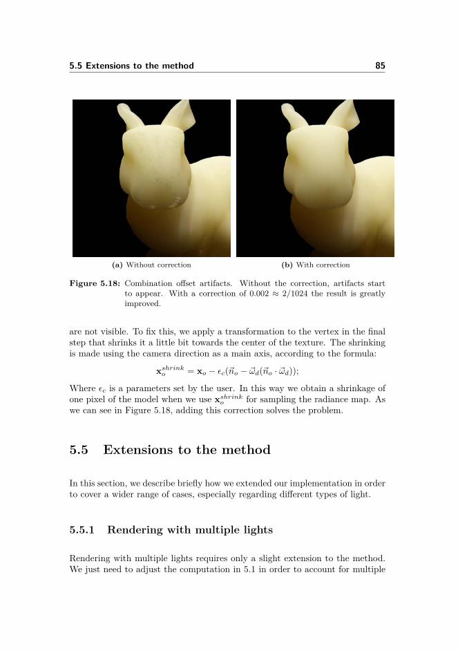
5.5 Extensions to the method 85

(a) Without correction (b) With correction

Figure 5.18: Combination offset artifacts. Without the correction, artifacts startto appear. With a correction of 0.002 ≈ 2/1024 the result is greatlyimproved.

are not visible. To fix this, we apply a transformation to the vertex in the finalstep that shrinks it a little bit towards the center of the texture. The shrinkingis made using the camera direction as a main axis, according to the formula:

xshrinko = xo − εc(~no − ~ωd(~no · ~ωd));

Where εc is a parameters set by the user. In this way we obtain a shrinkage ofone pixel of the model when we use xshrinko for sampling the radiance map. Aswe can see in Figure 5.18, adding this correction solves the problem.

5.5 Extensions to the method

In this section, we describe briefly how we extended our implementation in orderto cover a wider range of cases, especially regarding different types of light.

5.5.1 Rendering with multiple lights

Rendering with multiple lights requires only a slight extension to the method.We just need to adjust the computation in 5.1 in order to account for multiple

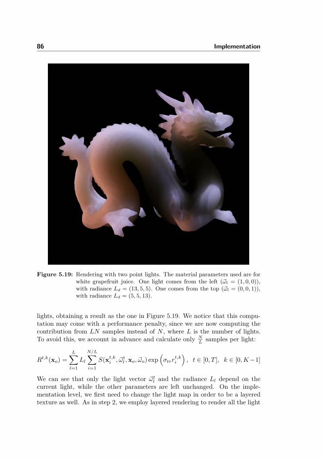
86 Implementation

Figure 5.19: Rendering with two point lights. The material parameters used are forwhite grapefruit juice. One light comes from the left (~ωl = (1, 0, 0)),with radiance Ld = (13, 5, 5). One comes from the top (~ωl = (0, 0, 1)),with radiance Ld = (5, 5, 13).

lights, obtaining a result as the one in Figure 5.19. We notice that this compu-tation may come with a performance penalty, since we are now computing thecontribution from LN samples instead of N , where L is the number of lights.To avoid this, we account in advance and calculate only N

L samples per light:

Rt,k(xo) =L∑l=1

Ll

N/L∑i=1

S(xt,ki , ~ωtl ,xo, ~ωo) exp(σtrr

t,ki

), t ∈ [0, T ], k ∈ [0,K−1]

We can see that only the light vector ~ωtl and the radiance Ll depend on thecurrent light, while the other parameters are left unchanged. On the imple-mentation level, we first need to change the light map in order to be a layeredtexture as well. As in step 2, we employ layered rendering to render all the light

5.5 Extensions to the method 87

maps at same time. Then we simply add an extra loop in the shader of step2 to account for multiple lights. As for the light parameters, they are passedto the shader as arrays of uniforms. The outline of the new shader illustratinghow lights are computed is listed in listing 5.12.

#version 430layout ( location = 0) out vec4 fragColor ;

[...] // constants , includes , textures omitted

uniform sampler2DArray vtex; // texture with verticesuniform sampler2DArray ntex; // texture with normals

smooth in vec3 position ;smooth in vec3 norm;

uniform vec4 light_pos [ MAX_LIGHTS ];uniform vec4 light_diff [ MAX_LIGHTS ];uniform int light_number ;uniform mat4 lightMatrices [ MAX_LIGHTS ];

[...] // BSSRDF code , uniform and functions

void main(void){

vec3 xo = position ;vec3 no = normalize (norm);

[...] // sampling the old color , noise calculation

for(int k = 0; k < light_number ; k++){

vec3 wi = light_pos [k]. xyz;vec4 light_post = lightMatrices [k] * vec4(xo ,1.0f);vec2 circle_center = light_post .xy;vec3 Li = light_diff [k]. xyz;

for(int i = 0; i < max_samples ; i++){

[...] // sampling from layer k in textures vtex and ntex[...] // summing over BSSRDF on vector accumulate

}}

fragColor = vec4( accumulate ,1.0f);[...] // adding old color

}

Listing 5.12: Outline of the shader in step 2 with support for multiple lights.

88 Implementation

5.5.2 Rendering with other kinds of light

Our method does not depend on a specific type of light in order to render amaterial. Once we have a formula for the radiance for the light, we can simplyintroduce it in equation 5.1 and compute the result. So, for example, for a pointlight the equation would become.

Rt,k(xo) = Il

N∑i=1

S(xt,ki , xl−xi‖xl−xi‖ ,xo, ~ωo)‖xl − xi‖

exp(σtrr

t,ki

), t ∈ [0, T ], k ∈ [0,K−1]

(5.4)Where xl is the light position and Il the light intensity. More generally, if wehave a function to compute the light direction ~ωl(xi) and a function to computeradiance L(xi, ~ωl(xi)) we can express equation 5.1 in the following way:

Rt,k(xo) =L∑l=1

N/L∑i=1

Lt(xi, ~ωl(xi))S(xt,ki , ~ωtl (xi),xo, ~ωo) exp(σtrr

t,ki

)If we have only point and directional lights, we have the following setup for thetwo formulas:

~ωl(xi) ={~ωl if l is directional with ~ωl, Ll

xl−xi‖xl−xi‖ if l is point with xl, Il

L(xi, ~ωl(xi)) ={Ll if l is directional with ~ωl, Ll

Il‖xl−xi‖ if l is point with xl, Il

On the implementation level, we can still use same uniforms that we use formultiple lights: the position vector will become either the position of the di-rection of the light. We make the position vector of the light carry some extrainformation in the alpha channel: if the alpha is zero (i.e. the vector is of type(x, y, z, 0)), we are dealing with a directional light, while if the alpha is one (i.e.the vector is of type (x, y, z, 1)) we are using a point light. The code to calculatelights thus becomes:

int current_light = k;vec3 wi = light_pos [ current_light ]. xyz;vec4 rad = light_diff [ current_light ];vec3 topoint = wi - xo;float light_type = light_pos [ current_light ].a;wi = ( light_type > 0)? normalize ( topoint ) : normalize (wi);vec3 Li = light_diff [ current_light ]. xyz;Li = ( light_type > 0)? Li / dot(topoint , topoint ) : Li;

Listing 5.13: GLSL Code to calculate the radiance Li and the incoming lightdirection wi for the k-th directional or point light source.

5.5 Extensions to the method 89

(a) Directional: ~ωl = (0, 0, 1) Ld = 25 (b) Point: xl = (0, 0, 2) Id = 60

Figure 5.20: Rendering with a directional and a point light. The material parametersare the ones for potato.

5.5.3 Rendering with environment light illumination

As for the environment lighting, we proceed as we outlined in Section 4.4. Inthe method chapter, we omitted how we do actually organize and sample ourCDF. The idea is to have one CDF for the rows of the function that gives usthe CDF according to the probability pu(u). Then we have a CDF for eachone of the column of the functions, that sample the probability pv(v|u). Whenwe select a random couple of random points (ζ1, ζ2) we first sample the firstfunction according to ζ1, then we sample the resulting column using ζ2.

We define our discrete CDF as and array C of s+ 1 elements as follows, wheres is the size of the distribution P (that would be either n or m in our case). Pis an array of N elements.

C[i] =∑i−1k=0 C[k] + P [i]

s C[s]

Then, we sample our CDF using a generic value ζ using the following:

u = j + ζ − C[j]C[j + 1]− C[j]

Where j = minj{j ∈ [0, s] | C[j] > ζ} − 1 is the CDF value right before theCDF surpasses ζ. This is basically the inverse function we discussed in Section

90 Implementation

Figure 5.21: Rendering a dragon using sixteen directional lights generated from theDoge map (with reflection). The material parameters are a potatomaterial.

4.4. Once we have calculated the two values (u1, u2), as before we convertthem to spherical coordinates, from which we create a set of directional lightsthat approximate our environment light. We can appreciate the rendering withdifferent numbers of generated lights using the doge light map in Figure 5.21.

5.6 Discussion

In this section, we anticipate some of the results that will be presented in Chap-ter 6, in order to analyze our method and present advantages and disadvantagesof the method, and more specifically of our implementation.

5.6 Discussion 91

5.6.1 Advantages

The great advantage of this method, that comes from the BSSRDF model, isthat it already accounts for self shadowing and self occlusion. So, no extra stepsare required in order to account for these effects, that usually are difficult toevaluate in a real-time fashion. Moreover, if we reuse the same light map forall the objects in the scene, it is possible to account for the occlusion betweenobjects. So, if an object is placed between the light and another object, a softshadow of the first object on the second one will appear. However, since thematerial properties are not stored in the light map, the contribution from theother points will use the same properties that we are using to render the object(so, another object will cast a ”potato shadow” on a potato object).

Another advantage of our method is that is tightly coupled with the shadowmapping pipeline. Shadow mapping is widely used nowadays in most of real timegraphics applications, so the cost of introducing our method is greatly reduced,since the light map data are usually available for use. In addition, the methodis generally adaptable to any kind of shadow mapping technique, providing thatit is able to store vertices and normals, and that those are accessible from steptwo in the algorithm. The cost of adding normal and vertex storage is usuallyonly heavy on the memory requirements, since the vertex position is calculatedanyway during the render to the shadow map.

Compared to other techniques for rendering translucent materials (such as vox-elization), our method has low memory requirements. As we will see, the size ofthe textures employed in the method should not be too big in order to achievea reasonable quality. This also comes from the fact that subsurface scatteringeffects are result of blurring of the incoming light, so a low size texture canrepresent the effects very well.

Finally, another advantage of the method is that the final step relies only on theknowledge of the exiting position and normal, so it can be integrated in both aforward and a deferred rendering pipeline, making it very flexible.

5.6.2 Disadvantages

The first and biggest disadvantage of this method is that one frame is givingonly an approximate and noisy approximation of the final result, that needs tobe blurred using mipmaps in order to get a smooth result. In addition, everytime something changed in the scene, the computations need to be redone everyframe, not allowing the method to ever reach convergence. In this case, ping

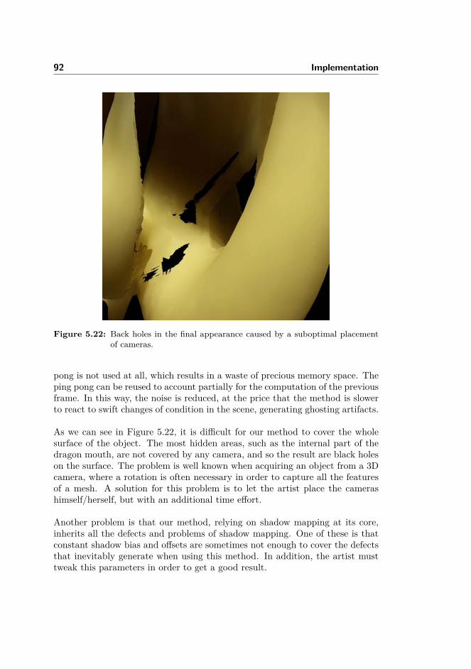
92 Implementation

Figure 5.22: Back holes in the final appearance caused by a suboptimal placementof cameras.

pong is not used at all, which results in a waste of precious memory space. Theping pong can be reused to account partially for the computation of the previousframe. In this way, the noise is reduced, at the price that the method is slowerto react to swift changes of condition in the scene, generating ghosting artifacts.

As we can see in Figure 5.22, it is difficult for our method to cover the wholesurface of the object. The most hidden areas, such as the internal part of thedragon mouth, are not covered by any camera, and so the result are black holeson the surface. The problem is well known when acquiring an object from a 3Dcamera, where a rotation is often necessary in order to capture all the featuresof a mesh. A solution for this problem is to let the artist place the camerashimself/herself, but with an additional time effort.

Another problem is that our method, relying on shadow mapping at its core,inherits all the defects and problems of shadow mapping. One of these is thatconstant shadow bias and offsets are sometimes not enough to cover the defectsthat inevitably generate when using this method. In addition, the artist musttweak this parameters in order to get a good result.

5.6 Discussion 93

Finally, a defect that comes from the method we are using to generate thedirectional lights from the environment map generally has the problem that incertain radiance maps, where there are a lot of very bright spots. In these maps,it tends to account only for the very bright spots and thus not approximate theoverall result very well. In this case, a solution based on spherical harmonics[Sloan, 2008] environment lighting may be preferable.

94 Implementation

Chapter 6

Results

In the last chapter, we discussed the implementation of our method. In thischapter, we are going to check it after the assumptions we stated in chapter 1,discussing advantages, disadvantages, and trade-offs. In the first section, we willdiscuss the quality result of our method, comparing it to path-traced results. Inthe second section, we will discuss how close we can get to the expected resultsin the performance domain, testing it for different parameters.

6.1 Parameters

The parameters were introduced in the previous chapter 5. We will sum themup here, in order to have a reference for this chapter.

• M , the total number of points in the disk. We recall that we make a discof the size of the object bounding box and then generate M exponentiallybased samples in it. Unless otherwise stated, M = 1000

• q, the modifier of the exponential distribution of the samples. Unlessotherwise stated, q = 1.

• N , the number of samples used from the disc. It is always N < M .

96 Results

• K, the number of directions used in the radiance map. Unless otherwisestated, K = 16.

• L, the number of lights in the scene.

• Wl, the size in pixel of the light map. Unless otherwise stated, Wl = 512.

• Wr, the size in pixel of the radiance map. Unless otherwise stated, Wr =1024.

Other parameters are available in the method, such as all the parameters of thecameras. In this section, we listed only the parameters that makes sense for theuser to tweak, and that can directly influence the quality or the performance ofthe final result.

6.2 Quality comparisons

In the domain of quality, we compared our method to offline rendered solutions,always made using the directional dipole. The solutions are compared onlyvisually, since if was not possible to perfectly match the perspective and viewcameras of the original pictures. We will see that the visual results of ourmethod, given enough samples, can produce a result comparable to the one of aoffline rendered solution. We will compare our results at convergence (after 100frames of evolution), unless otherwise stated.

6.2.1 Optimal radius

In section 5.3.4.1, we discussed how to generate exponentially biased points inour implementation. In our algorithm, to choose how to distribute the samplingpoints, we adopt the strategy of choosing a distribution biased towards thefollowing exponent:

σ∗ = min(σtr,x, σtr,y, σtr,z)q

We can see why we use the minimum coefficient in Figures 6.1 and 6.2. σtr as acoefficient, is related to how much the scattering effects propagate. If we look atthe directional dipole formula in 3.13, we can see that the dipole has a leadingterm depending on e−σtrt. If we consider only this term, the average distancethe light travels in the medium is 1/σtr. Figure 6.1 shows these radii for thepotato and the ketchup material. So, in order to account for all channels in

6.2 Quality comparisons 97

our sampling, we need choose as a exponent for our sampling pdf the maximumradius:

max(

1σtr,x

,1

σtr,y,

1σtr,z

)= min(σtr,x, σtr,y, σtr,z)

And this is how we obtain Equation 6.2.1. We will see in the next section thatthe q parameter in the equation is necessary in order to allow better performancewith a fewer number of samples. In Figure 6.2 we can see the effects of choosingdifferent radii according to the three coefficients in ketchup. When we use thered radius, all the effects are accounted for. When we use the green radius, welose the red absorption part. If we use the blue channel, the green and the redpart of the absorption spectrum disappear, resulting in a gray/blue appearance.

(a) Potato (b) Ketchup

Figure 6.1: Average radius of which the scattering effects are important for ketchupand potato materials.

6.2.2 Tests with different number of samples

The material tested where:

• Potato, a highly scattering isotropic material (α = σs/σa ≈ 102),

• Marble, a even higher high scattering material (α ≈ 104)

• White grapefruit juice, a material with a big forward scattering component(α ≈ 102, g ≈ 0.5)

98 Results

(a) σ∗ = σtr,x (b) σ∗ = σtr,y (c) σ∗ = σtr,z

Figure 6.2: Bunny rendered with different radii. We can appreciate the differentabsorptions according to the distribution radius. N = 20, M = 160,q = 1 in all images.

• Ketchup, a material that has a strong absorption component in the redchannel (αred ≈ 10−2, αgreen ≈ αblue ≈ 102)

• Beer, a high absorption material with nearly no scattering.

We are biased against highly scattering material because those are the materialwhere our BSSRDF model gives our best results. However, we included materi-als as beer and ketchup to provide a comparison of our method even where theoriginal BSSRDF model should fail.

The first comparison we make is with the path traced spheres generated inFigure 4.6. The results are illustrated in Figure 6.3, comparing different valuesof M and N for a potato sphere. We can see that different values of M and Ngreatly influence the results. In fact, for a big M and the same N , the samplestend to be closer to the exiting point xo, so the results are more accurate on thehighlight region. If instead we chose a relatively small M , the points are widelyspread on the surface, to the absorption of the material is accounted for more.This results in a sphere with gradients that are closer to the reference. In thiscase, the highlights are way more difficult to see.

The result that gets closer to the reference solution is the one where N = M =1000, but as we will see this values are unfeasible in the realm of performance,even for simple models. So, it is the artist that should find the right balancebetween M and N in order to get a satisfying result.

In the next set of experiments, we can see the utility of the q parameter. Wetested a sphere of white grapefruit juice in Figure 6.4, a material with a high

6.2 Quality comparisons 99

(a) N = 120, M = 120 (b) N = 120, M = 300 (c) N = 300, M = 300

(d) N = 120, M = 1000 (e) N = 300, M = 1000 (f) N = 1000, M = 1000

(g) Path traced solution

Figure 6.3: Path traced rendering on a sphere of potato material compared with theresults of our method. The parameters are from table 4.1.

100 Results

forward scattering component. In this case we can see that that with a smallernumber of samples N = 100 and a q = 3 we can approximate very well thesolution where N = 1000 and q = 1, way more expensive for the GPU. In a testwith marble, in Figure 6.5 we can see that our sampling introduces artifacts, es-pecially on the color transition area. In this case, q slightly relieves the artifactsgenerated from the sampling.

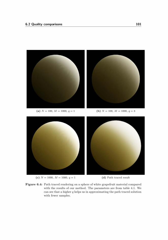
6.2 Quality comparisons 101

(a) N = 100, M = 1000, q = 1 (b) N = 100, M = 1000, q = 3

(c) N = 1000, M = 1000, q = 1 (d) Path traced result

Figure 6.4: Path traced rendering on a sphere of white grapefruit material comparedwith the results of our method. The parameters are from table 4.1. Wecan see that a higher q helps us in approximating the path traced solutionwith fewer samples.

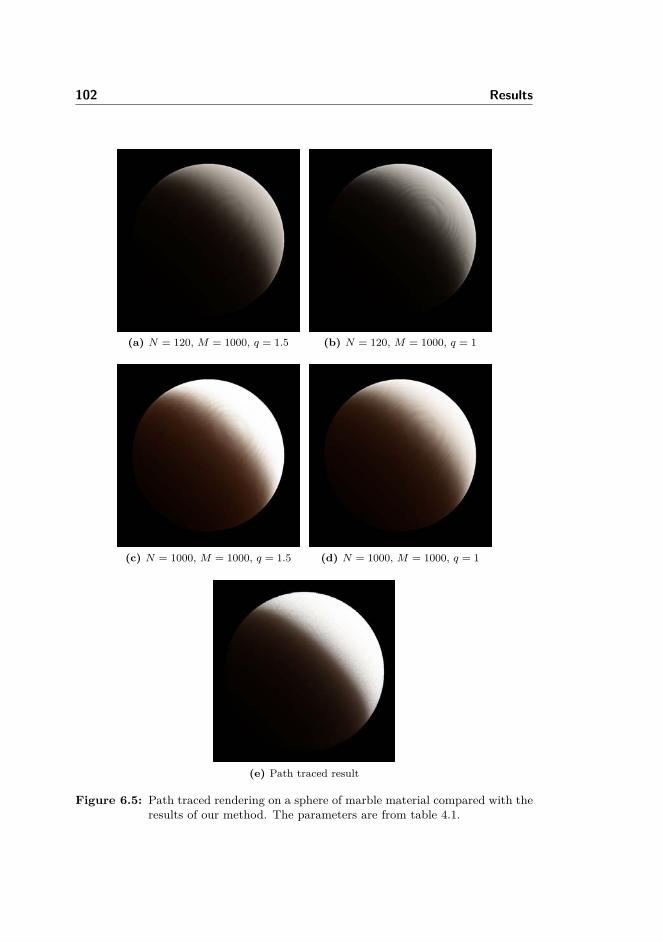
102 Results

(a) N = 120, M = 1000, q = 1.5 (b) N = 120, M = 1000, q = 1

(c) N = 1000, M = 1000, q = 1.5 (d) N = 1000, M = 1000, q = 1

(e) Path traced result

Figure 6.5: Path traced rendering on a sphere of marble material compared with theresults of our method. The parameters are from table 4.1.

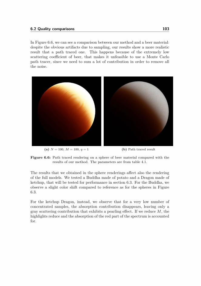
6.2 Quality comparisons 103

In Figure 6.6, we can see a comparison between our method and a beer material:despite the obvious artifacts due to sampling, our results show a more realisticresult that a path traced one. This happens because of the extremely lowscattering coefficient of beer, that makes it unfeasible to use a Monte Carlopath tracer, since we need to sum a lot of contribution in order to remove allthe noise.

(a) N = 100, M = 100, q = 1 (b) Path traced result

Figure 6.6: Path traced rendering on a sphere of beer material compared with theresults of our method. The parameters are from table 4.1.

The results that we obtained in the sphere renderings affect also the renderingof the full models. We tested a Buddha made of potato and a Dragon made ofketchup, that will be tested for performance in section 6.3. For the Buddha, weobserve a slight color shift compared to reference as for the spheres in Figure6.3.

For the ketchup Dragon, instead, we observe that for a very low number ofconcentrated samples, the absorption contribution disappears, leaving only agray scattering contribution that exhibits a pearling effect. If we reduce M , thehighlights reduce and the absorption of the red part of the spectrum is accountedfor.

104 Results

(a) N = 100, M = 1000, q = 1 (b) N = 200, M = 1000, q = 1

(c) N = 100, M = 300, q = 1 (d) Path traced result

Figure 6.7: Rendering of a potato Buddha using the directional dipole, with increas-ing number of samples.

6.2 Quality comparisons 105

(a) N = 10, M = 100, q = 1.5 (b) N = 50, M = 120, q = 1

(c) N = 50, M = 1000, q = 1.5 (d) Path traced result

Figure 6.8: Rendering of a ketchup Dragon using the directional dipole, with chang-ing values of M and N .

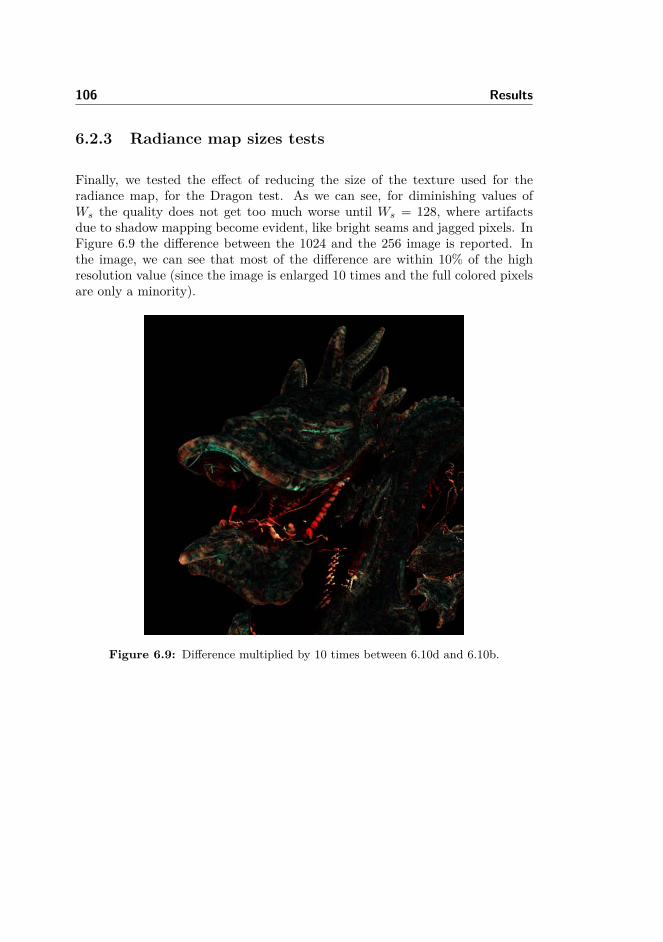
106 Results

6.2.3 Radiance map sizes tests

Finally, we tested the effect of reducing the size of the texture used for theradiance map, for the Dragon test. As we can see, for diminishing values ofWs the quality does not get too much worse until Ws = 128, where artifactsdue to shadow mapping become evident, like bright seams and jagged pixels. InFigure 6.9 the difference between the 1024 and the 256 image is reported. Inthe image, we can see that most of the difference are within 10% of the highresolution value (since the image is enlarged 10 times and the full colored pixelsare only a minority).

Figure 6.9: Difference multiplied by 10 times between 6.10d and 6.10b.

6.2 Quality comparisons 107

(a) Ws = 128 (b) Ws = 256

(c) Ws = 512 (d) Ws = 1024

Figure 6.10: Rendering of a ketchup Dragon using the directional dipole, with vary-ing radiance map size Ws.

108 Results

6.2.4 Tests of mipmap blurring quality

In this part we tested the quality improvement from the mipmap blurring intro-duced in section 5.4.2 to the final image. We can see the result of our method atthe first frame of our simulation for different mipmap levels. At the beginning ofthe evolution, a strong blurring (two passes) is needed to compensate the highlevel noise, as we can see from image 6.11. During the evolution, a lesser levelof mipmaps is needed in order to preserve a noiseless image. At convergence,we do not need mipmap blurring at all, as the result converge to the solution.

(a) Mipmap level 0 (no blur) (b) Mipmap level 1

(c) Mipmap level 2 (d) Convergence

Figure 6.11: Detail of a potato Dragon in the first frame of the computation fordifferent mipmap levels. We can see that the second mipmap levelis very close to the final result. However, some artifacts due to thestretching of the mipmap appear, such as black spots and bright seams.All the Figures use N = 32 and M = 300.

6.2 Quality comparisons 109

6.2.5 Environment map illumination

All the given consideration so far are the same irregardless if we have an envi-ronment map or a single directional light. In this section we present the resultsobtained we environment light illumination. Visually, we obtain a nice result.Obviously, since the samples are split between different lights, an overlapping isinevitable, and we need an higher number of samples to obtain a decent result.The Bunny in Figure 6.12 was obtained using 16 directional lights, sampledusing the method in 5.5.3 and 4.4, with N = 80 (5 samples per light) andM = 1000.

As for reference, we compared our results to the reference image of the potatoBuddha from Frisvad et al. [2014] in Figure 6.13. We had to try to match thelight settings and the camera, but here as well we notice the same color shift asfor directional lights. Also in this case we used 16 directional lights to representour skybox.

Figure 6.12: Marble Bunny rendered in the Doge environment map. Note that thelight is predominantly from the up direction.

110 Results

(a) L = 16, N = 90, M = 1000 (b) L = 16, N = 90, M = 320

(c) L = 16, N = 90, M = 160 (d) Hierarchical integration

Figure 6.13: Rendering of a potato Buddha using our environment lighting and theUffizi map.

6.2 Quality comparisons 111

In the image of Figure 6.14, we compare the result using the Pisa Courtyardenvironment map on a Stanford Dragon, comparing a different number of lights.We can see the more lights we introduce, the more closer we get to a result thatapproximate true environment illumination. We observe also that the imageshave more scattering than absorption the more we increase the number of lights:this is because the total number of samples N does not change, so each light hasless and less samples available. In this way, the samples tend to concentrate inthe center and produce a result where the scattering component is predominant.

(a) 2 lights (b) 4 lights

(c) 8 lights (d) 16 lights

Figure 6.14: Rendering of a potato Dragon (N = 32, M = 170) using a differentnumber of directional light to represent the environment map.

112 Results

6.3 Performance tests

In this section, we examine and analyze the performance of our method. Thetests in this section were made by keeping in mind the performance requirementswe made in chapter 1, and they exploit how the different parameters listed in6.1 influence the final result. For the tests, we used three main models, to whichwe will refer as Bunny, Dragon and Buddha (see table 6.1). The models cover avarying range of complexity. The Bunny model represents a typical model usedin modern games and consoles (104 triangles), while the Dragon represents ahighly detailed model, usually for visualization purposes (105 triangles). Finally,the Buddha model represent a high resolution model, and it will be used as astress test for our algorithm (106 triangles).

Model Vertices (#V ) Triangles (#∆)

Bunny 3581 21474 ≈ 104

Dragon 50000 300000 ≈ 105

Buddha 549409 3262422 ≈ 106

Table 6.1: The three models used for our tests, with number of vertices and triangles.

All the tests were performed on a NVIDIA GeForce GTX 780Ti, a high-endmodern GPU with OpenGL 4.3 capabilities. All the timings measure the av-erage milliseconds during the 20th and the 40th frame during an evolution toconvergence of 100 frames. The first frames were not measured because of theoverhead introduced by the initialization procedure (texture creation, modelparsing and loading, shader compilation, etc.).

6.3.1 Time algorithm breakdown

The first test we are going to perform is to time how much time the algorithmtakes to perform the different steps illustrated in chapter 5. When we weretiming the algorithm, we divided the whole computation into five different steps:

1. Initialization phase, where all the different constants and data structuresin the algorithm are created and initialized.

2. Render to light map step, that corresponds to step 1 in our outline.

6.3 Performance tests 113

3. Render to radiance map step, that corresponds to step 2 in our outline.

4. Mipmap generation, as in the extension outlined in section 5.4.2.

5. Final render combination, that corresponds to step 3 in our outline.

For this tests we tried all the three models, and the results are shown in Figure6.15. The parameters were tweaked in order to reach the best compromisebetween visual quality and performance, in order to measure realistic timings.

We can observe that, irregardless of the test case, most of the time is spentcomputing the BSSRDF function for the samples in step 2. Thee render tolightmap step does not have a big performance impact, likely because all thetests were made with one light. We will test in the next section the impact ofa different number of lights on the performance. Another consideration to dois that, as to be expected, the more triangles we have the less samples we canuse. As we will see, this is not the only factor that causes a performance drop.However, the big number of triangles that has to be multiplied by the numberof directions generates a big load on the GPU for rasterization procedures.

Regarding the mipmap generation, as expected its performance is not tied tothe size of the model, but only to the size of the radiance map texture Ws andto the number of mipmaps we generate. Finally, the final combination step istied as well to the size of the model, rising slightly with an increasing modelsize. However, in this case we are rendering only once the model to the mainframebuffer, and not K times as in step 2.

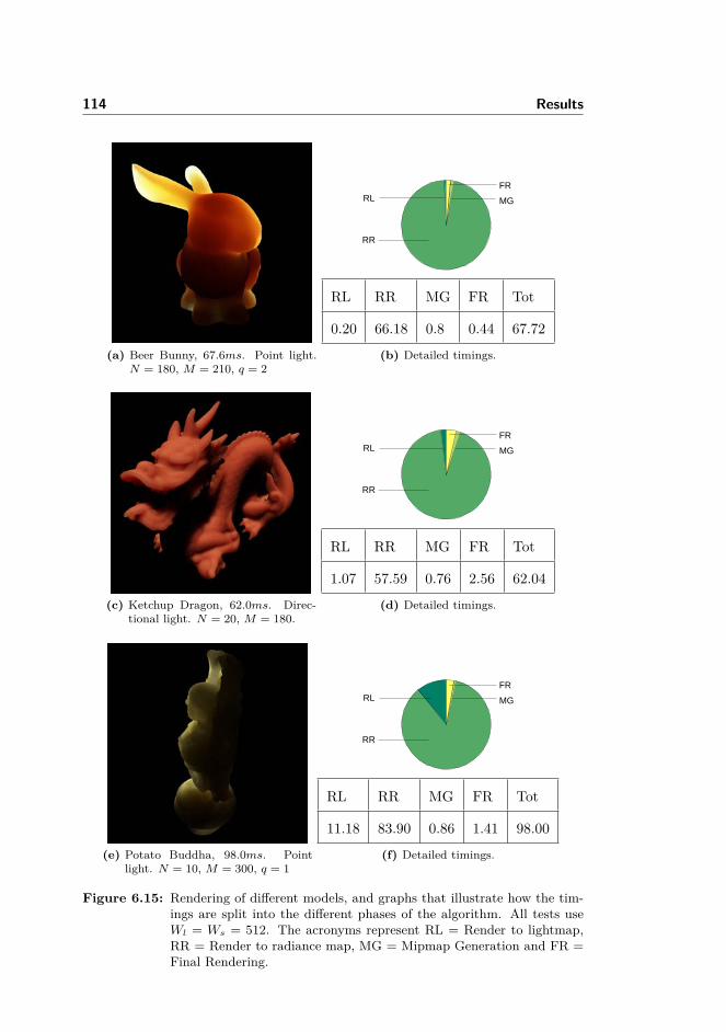
114 Results

(a) Beer Bunny, 67.6ms. Point light.N = 180, M = 210, q = 2

RR

MGRLFR

RL RR MG FR Tot

0.20 66.18 0.8 0.44 67.72(b) Detailed timings.

(c) Ketchup Dragon, 62.0ms. Direc-tional light. N = 20, M = 180.

RR

MGRLFR

RL RR MG FR Tot

1.07 57.59 0.76 2.56 62.04(d) Detailed timings.

(e) Potato Buddha, 98.0ms. Pointlight. N = 10, M = 300, q = 1

RR

MGRLFR

RL RR MG FR Tot

11.18 83.90 0.86 1.41 98.00(f) Detailed timings.

Figure 6.15: Rendering of different models, and graphs that illustrate how the tim-ings are split into the different phases of the algorithm. All tests useWl = Ws = 512. The acronyms represent RL = Render to lightmap,RR = Render to radiance map, MG = Mipmap Generation and FR =Final Rendering.

6.3 Performance tests 115

6.3.2 Tests for varying parameters

In this section, we will discuss how well our method behaves for changing pa-rameters. From the quality tests before we have learned that the parametersthat are related mostly to the quality of the are N , M , q and to a certain extentWs. The number of directions K is important in order to ensure to cover thewhole model, and if we are generating the cameras automatically it cannot betoo low. Of the mentioned parametrs, M and q do not directly influence per-formance, as they are used only at the beginning of the computation in orderto distribute the points on the disc.

N parameterWe start by discussing N . We can see the results for different value of theparameter in the following table:

Number of samples (N)

Model #∆ 1 10 50 100

Bunny 104 2.1 5.3 19.8 38.2

Dragon 105 12.5 35.2 140.6 275.3

Buddha 106 96.7 97.7 128.0 216.0

Table 6.2: Timings in milliseconds of our method for different models and numberof samples N (potato material properties). The other parameters wereL = 1, Ws = Wl = 512, M = 1000, K = 16.

We tested N in the range 1 − 100. The test with N = 1 was introduced tomeasure the baseline performance of the method (where the most expensiveoperation is the generation of the random number for the rotation). We did notuse zero samples because otherwise the shader compiler optimizations wouldhave removed the base code as well, making the results not significant.

We note that from the graph the time to render the Dragon with 50 samples isslower that rendering the Buddha with the same parameters, despite the Buddhahaving 10 times the triangles as the Dragon. This suggests that N and thetriangle size of the model are not the only factors involved in the performance.Since the heavy computational step is made on a fragment shader in step 2, thenumber of pixels involved in the computation matters: the Buddha on averageoccupies less texture area on the directional cameras, and thus the number ofcomputations performed in total is less that the ones for the Dragon. For a lownumber of samples, the performance is bound by the rasterization time, so the

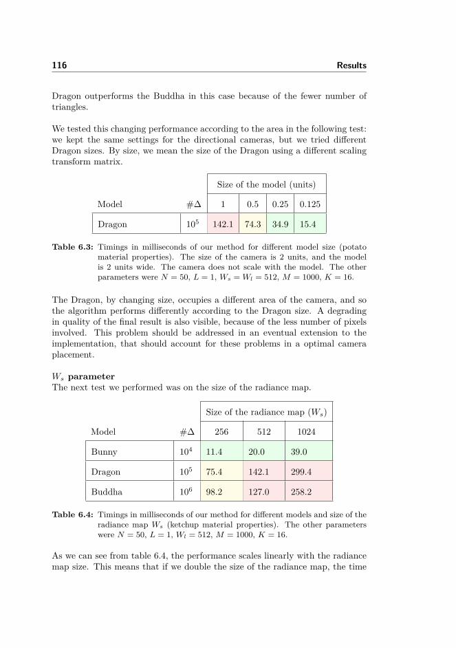
116 Results

Dragon outperforms the Buddha in this case because of the fewer number oftriangles.

We tested this changing performance according to the area in the following test:we kept the same settings for the directional cameras, but we tried differentDragon sizes. By size, we mean the size of the Dragon using a different scalingtransform matrix.

Size of the model (units)

Model #∆ 1 0.5 0.25 0.125

Dragon 105 142.1 74.3 34.9 15.4

Table 6.3: Timings in milliseconds of our method for different model size (potatomaterial properties). The size of the camera is 2 units, and the modelis 2 units wide. The camera does not scale with the model. The otherparameters were N = 50, L = 1, Ws = Wl = 512, M = 1000, K = 16.

The Dragon, by changing size, occupies a different area of the camera, and sothe algorithm performs differently according to the Dragon size. A degradingin quality of the final result is also visible, because of the less number of pixelsinvolved. This problem should be addressed in an eventual extension to theimplementation, that should account for these problems in a optimal cameraplacement.

Ws parameterThe next test we performed was on the size of the radiance map.

Size of the radiance map (Ws)

Model #∆ 256 512 1024

Bunny 104 11.4 20.0 39.0

Dragon 105 75.4 142.1 299.4

Buddha 106 98.2 127.0 258.2

Table 6.4: Timings in milliseconds of our method for different models and size of theradiance map Ws (ketchup material properties). The other parameterswere N = 50, L = 1, Wl = 512, M = 1000, K = 16.

As we can see from table 6.4, the performance scales linearly with the radiancemap size. This means that if we double the size of the radiance map, the time

6.3 Performance tests 117

to render the model roughly doubles. This comes from the fact that most of thetime in the computation is spent in rendering to the radiance map, that is a pixelbound operation. So if we double the size of map, we roughly double the numberof pixels involved and thus the number of the fragment shader invocations instep 2.

K parameterThe next test is about the number of directions used to render the model, K.

Number of directions (K)

Model #∆ 4 8 16 32

Bunny 104 6.6 10.0 20.1 42.1

Dragon 105 36.7 70.1 143.0 306.2

Buddha 106 32.5 55.8 128.3 363.5

Table 6.5: Timings in milliseconds of our method for different models and differentnumber of directions K (ketchup material properties). The other param-eters were N = 50, L = 1, Ws = Wl = 512, M = 1000, q = 1.

We can see that the performance for the models scales linearly. We can seefrom this test that is a big advantage to place the cameras manually, instead ofrelying on an automatic algorithm. A careful placement of the cameras can coverthe whole model evenly with a smaller number of cameras that an automaticplacement. In our implementation, we needed to use at least 16 cameras toensure that most of the models were covered. On the other hand, with carefulplacement of the cameras, we were able to lower the number of cameras up to8 in all cases, thus doubling the performance. Also in this test, we can see thatthe minor area occupation of the Buddha improves its performance for 4,8, and16 directions. For 32 directions, the number of triangles that actually need tobe rasterized (32 · 106) probably becomes so high that memory issues on theGPU become important.

Different types of lightsWe tested the different times in performance for different kind of lights. Sincethe operations performed are roughly the same (the point light requires an extradivision), also is the performance:

We times a third case, that is when we strip the outer loop in listing 5.12, thusobtaining a shader suitable for only one light. In this case, we can see that theperformance slightly improves by fractions of a millisecond.

118 Results

Type of light

Model #∆ Point light Directional light No loop

Dragon 105 61.8 60.3 60.1

Table 6.6: Timings in milliseconds of our method for different types of light (potatomaterial properties), one light. The other parameters were N = 20, Ws =Wl = 512, M = 1000, K = 16.

Different materialsWe finally tried to see if different materials gave a different performance onthe method. As we expected, the material does not influence the renderingtime, as the computations in the BSSRDF do not actually take advantage onthe material type to easy any computation. We can see the test result in thefollowing table:

Material

Model #∆ Ketchup Beer White grapefruit Potato

Dragon 105 61.7 61.6 62.0 62.1

Table 6.7: Timings in milliseconds of our method for different materials. The otherparameters were N = 20, L = 1, Ws = Wl = 512, M = 300, K = 16.

6.3 Performance tests 119

6.3.3 Tests on environment lighting

The considerations so far discussed apply also in environment map lighting,that we converted to a certain number L of directional lights. So discussingthe impact on performance of multiple lights and the impact of environmentlighting is essentially the same, apart from a initialization delay to generate thelights from the environment map that we will not consider.

The timings for different kind of lights are reported in the following table: As

Number of lights L

Model #∆ 1 2 4 8 16

Dragon 105 96.6 98.0 100.0 103.8 110.5

Table 6.8: Timings in milliseconds of our method for different number of lights (envi-ronment map approximation, material properties for potato). The otherparameters were N = 32, Ws = Wl = 512, M = 300, K = 16.

we can see, even if we maintain the same number of samples (N = 32, so thenumber of samples per light changes) the performance worsen increasing thenumber of lights. To look at this into more detail, we broke down the timingsagain in the different steps. We can see in Figure 6.16 that the increase in timingis due to step 1, the render to lightmap: in fact, we have to render the modelonce for each light, that implies a performance penalty.

1c 2c 4c 8c 160

5

10

15

Numbercofclights

Ren

derin

gctim

ec[m

s]

InitializationRenderctoclightcmapRenderctocradiancecmapMipmapcgenerationCombination

Figure 6.16: Rendering times for the environment lighting of Figure 6.8, split intothe various components. The rendering times of step 2 are not shown,but they are [91.8 93.3 93.5 95.0 97.1].

120 Results

Chapter 7

Future work

In this chapter we discuss the improvements that can be done to our method inorder to improve the solution.

7.1 Improving the quality

As we have seen the results section, catching the right effect balancing absorp-tion and scattering requires a lot of tweaking of the parameters M and q. Thisdepends from the fact that an exponential sampling based on σtr is not prob-ably the best suited for the solution, thus providing good results. A furtherinvestigation of optimal sampling patterns would be required in order to obtainfaithful results.

An idea we would like to explore is to use two separate disks with a differ-ent sampling radius, one accounting the absorption and one for the scatteringcontribution. The size of the radius of the two disk should be related to thescattering parameters, such as σa and σs. Further investigation is required inthis realm in order to obtain results applicable to a wide range of participatingmedia.

122 Future work

Another direction we would like to explore is the automatic placing of the cam-eras. Because of the variety and possible concavity of meshes, it is very difficultto place cameras in a way to ensure the complete coverage of the object. Thefield in which to find ideas in order to fully cover the object would be 3D meshacquisition using cameras. In this way, it will be possible for a user to avoid thetedious operation of placing the cameras in order to get a full coverage of theobject.

Another possibility in this area is to rotate the cameras during the renderingphase: in this case, fewer cameras will be necessary, but then an accumulationprocess would not be possible in the way we implemented it. It would require agreat change to the way the algorithm works in order to get a solution.

7.2 Improving the performance

Regarding the implementation, we tought about some possible extensions inorder to make the implementation faster and more reliable.

...

...

+

Initialization

Random number generation

BSSRDF calculation for N

samples

Draw call

Storage into radiance map

Figure 7.1: Different approaches to rendering to the radiance map: on the left, ourapproach (one random number generation, multiple samples in the sameshader invocation). On the right, the proposed approach: smaller shaderinvocations, that can be distributed on the GPU.

The first thing we have thought about would be to change the loop in step 2. Theidea would be to have instead to have a single fragment shader invocation withcycling N times on the samples, to have N separate fragment shader invocationsthat calculate the result. The single invocations can be summed over usingblending or atomic operations available since OpenGL 4.2. This would allowthe GPU more flexibility in scheduling its work. However, we have seen in 7.1

7.2 Improving the performance 123

that also the random number generation is an expensive operation for the GPU,and that would have to be repeated for each of the N fragments, potentiallyundermining the advantages of GPU scheduling.

Another improvement in order to make the performance more reliable wouldbe to make the cameras more adaptive. At the moment, the size of the lightand directional cameras is fixed and set up by the user. A simple extensionto the method would be to make the camera size adaptive, in order to adaptto the object bounding box. This would make the area in the radiance maptexture space more consistent regarding to the size of the object, leading to amore predictable result.

124 Future work

Chapter 8

Conclusions

In this thesis, we have presented an approch to rendering translucent materialsusing a new directional subsurface scattering BSSRDF models. We focused oncreating a method that renders translucent materials in real-time, thus approx-imating well path traced results.

In Chapter 2 we gave an overview of the different approaches to rendering sub-surface scattering in literature, identifying the gap in the knowledge in renderingtranslucent materials efficiently using a directional approach.

In Chapter 3, we instroduced the mathematical concepts that are needed to givea basic understanding of light transport theory and BSSRDF models, introduc-ing the nthe formulation of two BSSRDF dipole models, the standard dipolemodel and the directional dipole model. Using this knowledge, we gave thereader a theoretical introduction to our method, as well as scattering parame-ters and how they are acquired in Chapter 4. Chapter 4 provided an essentialbridge between theory and implementation, that we described in Chapter 5.In the implementation, we described a method that employs the advantages ofthe formulation of the directional dipole in order to create a robust methodthat implements the directional dipole taking advantage of the GPU renderingpipeline.

In Chapter 6, we compared our result to path traced solutions, proving that

126 Conclusions

our method can produce results that approximate well path-traced solutions,providing speed ups of four order of magnitude compared to path tracing onCPU. We also proved that our method for models of the size commonly used inthe computer game industry performs in real-time on a high-end modern GPU,limiting the size of memory used to a minimum.

Finally, in Chapter 7, we introduced some possible ideas to expand our methodin order to produce a higher quality result retaining its real-time capabilities.

To sum up, we think that most of the goals of the thesis stated in the intro-duction Chapter have been satisfied. This thesis hopefully provides an insighton a new way to approach the efficient rendering of translucent materials usingdirectional subsurface scattering.

Appendix A

Model matrices

In this chapter, we report the different model, view and projection matricesformulas we used in our mater thesis.

A.1 Model matrices

Translation matrix

T (t) =

1 0 0 tx0 1 0 ty0 0 1 tz0 0 0 1

Rotation matrix

Rx(θ) =

1 0 0 00 cos θ − sin θ 00 sin θ cos θ 00 0 0 1

128 Model matrices

Ry(θ) =

cos θ 0 sin θ 0

0 1 0 0− sin θ 0 cos θ 0

0 0 0 1

Rz(θ) =

cos θ − sin θ 0 0sin θ cos θ 0 0

0 0 1 00 0 0 1

Scale matrix

S(s) =

sx 0 0 00 sy 0 00 0 sz 00 0 0 1

A.2 View Matrix

e is the camera position, d is the camera direction, u is the up vector.

~c = − d‖d‖

~a = ~c× u‖~c× u‖

~b = ~a× ~c

V (e,d,u) =

~ax ~ay ~az −ex~bx ~by ~bz −ey~cx ~cy ~cz −ez0 0 0 1

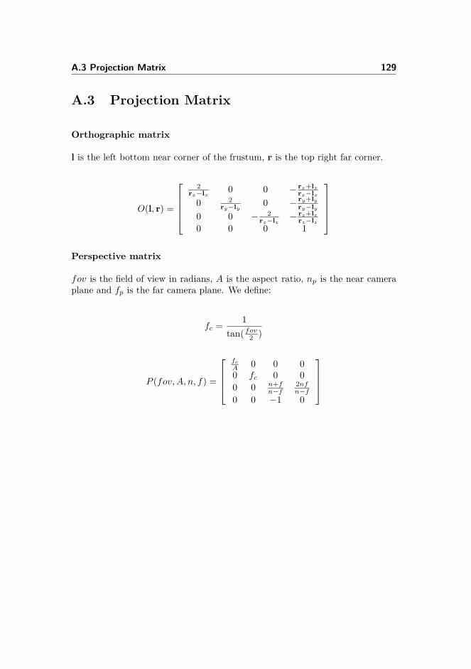
A.3 Projection Matrix 129

A.3 Projection Matrix

Orthographic matrix

l is the left bottom near corner of the frustum, r is the top right far corner.

O(l, r) =

2

rx−lx 0 0 − rx+lxrx−lx

0 2ry−ly 0 − ry+ly

ry−ly0 0 − 2

rz−lz − rz+lzrz−lz

0 0 0 1

Perspective matrix

fov is the field of view in radians, A is the aspect ratio, np is the near cameraplane and fp is the far camera plane. We define:

fc = 1tan( fov2 )

P (fov,A, n, f) =

fcA 0 0 00 fc 0 00 0 n+f

n−f2nfn−f

0 0 −1 0

130 Model matrices

Appendix B

Directional dipole GPU code

const float EPSILON_MU = 0.0f;const vec3 one = vec3 (1.0f);

vec3 S_infinite (vec3 _r , vec3 _r_sq , float x_dot_w12 , float no_dot_w12 , ←↩float x_dot_no )

{vec3 _r_tr = transmission * _r;vec3 _r_tr_p1 = _r_tr + one;vec3 _T = exp(- _r_tr );vec3 coeff = _T / (_r * _r_sq );vec3 first = C_s * ( _r_sq * D_rev + 3 * _r_tr_p1 * x_dot_w12 );vec3 second = C_e * ( three_D * _r_tr_p1 * no_dot_w12 - ( _r_tr_p1 + ←↩

three_D * (3 * _r_tr_p1 + _r_tr * _r_tr ) / ( _r_sq ) * x_dot_w12 ) * ←↩x_dot_no );

vec3 _S = coeff * ( first - second );return _S;

}

vec3 S_infinite_vec (vec3 _r , vec3 _r_sq , vec3 x_dot_w12 , float no_dot_w12 , ←↩vec3 x_dot_no )

{vec3 _r_tr = transmission * _r;vec3 _r_tr_p1 = _r_tr + one;vec3 _T = exp(- _r_tr );vec3 coeff = _T / (_r * _r_sq );vec3 first = C_s * ( _r_sq * D_rev + 3 * _r_tr_p1 * x_dot_w12 );vec3 second = C_e * ( three_D * _r_tr_p1 * no_dot_w12 - ( _r_tr_p1 + ←↩

three_D * (3 * _r_tr_p1 + _r_tr * _r_tr ) / ( _r_sq ) * x_dot_w12 ) * ←↩x_dot_no );

vec3 _S = coeff * ( first - second );return _S;

}

132 Directional dipole GPU code

vec3 bssrdf (vec3 _xi ,vec3 _nin ,vec3 _wi ,vec3 _xo , vec3 _no){

vec3 _x = _xo - _xi;float r_sqr = dot(_x ,_x);vec3 _w12 = refract2 (_wi ,_nin);

float mu = -dot(_no , _w12);float dot_x_w12 = dot(_x ,_w12);float dot_x_no = dot(_x ,_no);

vec3 _r_sqr = r_sqr .xxx;vec3 _dr_sqr = _r_sqr ;

float edge = step(mu , EPSILON_MU ); // == 1.0 if mu > EPSILON_MUvec3 project = vec3(sqrt( r_sqr - dot_x_w12 * dot_x_w12 )/sqrt( _r_sqr + ←↩

de_sqr ));vec3 _D_prime = abs(mu) * D * edge + one_over_three_ext * (1.0f - edge)←↩

;_dr_sqr += _D_prime * ( _D_prime + two_de * project * edge);

vec3 _dr = sqrt( _dr_sqr );

float edge_nistar = step(abs( dot_x_no ) ,0.01f); // 1.0 if dot_x_no > ←↩0.01

vec3 _t = normalize ( cross (_nin ,_x));vec3 _nistar = _nin * edge_nistar + cross ( normalize (_x),_t) * (1.0f - ←↩

edge_nistar );

mat3 _xov = mat3(_x ,_x ,_x) - outerProduct (_nistar , two_a_de );vec3 _dv_sqr = vec3(dot(_xov [0] , _xov [0]) ,dot(_xov [1] , _xov [1]) ,dot(_xov←↩

[2] , _xov [2]));vec3 _dv = sqrt( _dv_sqr );vec3 _wv = _w12 - 2 * dot(_w12 , _nistar ) * _nistar ;

vec3 _x_dot_wv = _wv * _xov;vec3 _x_dot_no = _no * _xov;

vec3 _S_r = S_infinite (_dr , _dr_sqr , dot_x_w12 , -mu , dot_x_no );vec3 _S_v = S_infinite_vec (_dv , _dv_sqr , _x_dot_wv , dot(_no ,_wv), ←↩

_x_dot_no );vec3 _S = _S_r - _S_v;

_S *= fresnel_T (_wi ,_nin);_S = max(vec3 (0.0f),_S);

return _S;}

Listing B.1: Directional dipole code optimized for GPU. Uniforms and Fresnelformulas code is not reported.

Bibliography

Tomas Akenine-Moller, Eric Haines, and Natty Hoffman. Real-Time Rendering3rd Edition. A. K. Peters, Ltd., Natick, MA, USA, 2008.

Michael Ashikmin, Simon Premoze, and Peter Shirley. A microfacet-basedbrdf generator. In Proceedings of the 27th Annual Conference on ComputerGraphics and Interactive Techniques, SIGGRAPH ’00, pages 65–74, NewYork, NY, USA, 2000. ACM Press/Addison-Wesley Publishing Co. URLhttp://dx.doi.org/10.1145/344779.344814.

James Blinn. Models of light reflection for computer synthesized pictures. SIG-GRAPH Comput. Graph., 11(2):192–198, July 1977. URL http://doi.acm.org/10.1145/965141.563893.

Jesper Børlum, Brian Bunch Christensen, Thomas Kim Kjeldsen, Peter TrierMikkelsen, Karsten Østergaard Noe, Jens Rimestad, and Jesper Mosegaard.Sslpv: Subsurface light propagation volumes. In Proceedings of the ACMSIGGRAPH Symposium on High Performance Graphics, HPG ’11, pages 7–14, New York, NY, USA, 2011. ACM. URL http://doi.acm.org/10.1145/2018323.2018325.

Max Born and Wolf Emil. Principles of Optics. Cambridge University Press, 7edition, 1999.

Subrahmanyan Chandrasekar. Radiative Transfer. Oxford University Press,1950.

Michael Cohen, John Wallace, and Pat Hanrahan. Radiosity and Realistic ImageSynthesis. Academic Press Professional, Inc., San Diego, CA, USA, 1993.

Carsten Dachsbacher and Marc Stamminger. Translucent shadow maps. InProceedings of the 14th Eurographics Workshop on Rendering, EGRW ’03,

134 BIBLIOGRAPHY

pages 197–201, Aire-la-Ville, Switzerland, Switzerland, 2003. EurographicsAssociation. URL http://dl.acm.org/citation.cfm?id=882404.882433.

Boris Davison and John Bradbury Sykes. Neutron transport theory. OxfordUniversity Press, 1958.

Eugene D’Eon. A better dipole (a publicly available manuscript). Technical re-port, -, 2012. URL .http://www.eugenedeon.com/papers/betterdipole.pdf.

Eugene D’Eon and Geoffrey Irving. A quantized-diffusion model for renderingtranslucent materials. In ACM SIGGRAPH 2011 Papers, SIGGRAPH ’11,pages 56:1–56:14, New York, NY, USA, 2011. ACM. URL http://doi.acm.org/10.1145/1964921.1964951.

Eugene d’Eon, David Luebke, and Eric Enderton. Efficient rendering of hu-man skin. In Proceedings of the 18th Eurographics Conference on RenderingTechniques, EGSR’07, pages 147–157, Aire-la-Ville, Switzerland, Switzerland,2007. Eurographics Association. URL http://dx.doi.org/10.2312/EGWR/EGSR07/147-157.

Agns Desolneux, Lionel Moisan, and Jean-Michel Morel. From Gestalt Theoryto Image Analysis: A Probabilistic Approach. Springer Publishing Company,Incorporated, 1st edition, 2007.

Craig Donner. Towards Realistic Image Synthesis of Scattering Materials.PhD thesis, University of California, San Diego, La Jolla, CA, USA, 2006.AAI3226771.

Craig Donner and Henrik Wann Jensen. Light diffusion in multi-layered translu-cent materials. In ACM SIGGRAPH 2005 Papers, SIGGRAPH ’05, pages1032–1039, New York, NY, USA, 2005. ACM. URL http://doi.acm.org/10.1145/1186822.1073308.

Craig Donner, Jason Lawrence, Ravi Ramamoorthi, Toshiya Hachisuka, Hen-rik Wann Jensen, and Shree Nayar. An empirical bssrdf model. ACM Trans.Graph., 28(3):30:1–30:10, July 2009. URL http://doi.acm.org/10.1145/1531326.1531336.

Julie Dorsey, Alan Edelman, Henrik Wann Jensen, Justin Legakis, andHans Køhling Pedersen. Modeling and rendering of weathered stone. InProceedings of the 26th Annual Conference on Computer Graphics and In-teractive Techniques, SIGGRAPH ’99, pages 225–234, New York, NY, USA,1999. ACM Press/Addison-Wesley Publishing Co. URL http://dx.doi.org/10.1145/311535.311560.

D’Eon Eugene and Luebke David. Chapter 14. advanced techniques for realisticreal-time skin rendering. In GPU Gems 3. Addison-Wesley Professional, 2007.

BIBLIOGRAPHY 135

Cass Everitt, Ashu Rege, and Cem Cebenoyan. Hardware shadow mapping.Technical report, NVIDIA Corporation, 2003.

Raanan Fattal. Participating media illumination using light propagation maps.ACM Trans. Graph., 28(1):7:1–7:11, February 2009. URL http://doi.acm.org/10.1145/1477926.1477933.

Randima Fernando. GPU Gems: Programming Techniques, Tips and Tricks forReal-Time Graphics. Pearson Higher Education, 2004.

J. R. Frisvad, T. Hachisuka, and T. K. Kjeldsen. Directional dipole for sub-surface scattering in translucent materials. ACM Transactions on Graphics,2014, -:–, 2014. URL http://www2.imm.dtu.dk/pubdb/p.php?6646. To ap-pear.

Robin Green. Spherical harmonic lighting: The gritty details, January 2003.Sony Computer Entertainment America.

Simon Green. Chapter 16. real-time approximations to subsurface scattering.In GPU Gems: Programming Techniques, Tips and Tricks for Real-TimeGraphics. Pearson Higher Education, 2004.

J. H. Halton. Algorithm 247: Radical-inverse quasi-random point sequence.Commun. ACM, 7(12):701–702, December 1964. URL http://doi.acm.org.globalproxy.cvt.dk/10.1145/355588.365104.

Akira Ishimaru. Wave propagation and scattering in random media. IEEE, 1997.

ITU. Parameter values for the hdtv standards for production and internationalprogramme exchange. Technical Report ITU-R BT.709-2, ITU-R, June 2001.URL http://www.itu.int/rec/R-REC-BT.709-2-199510-S/en.

Henrik Wann Jensen and Juan Buhler. A rapid hierarchical rendering techniquefor translucent materials. ACM Trans. Graph., 21(3):576–581, July 2002. URLhttp://doi.acm.org/10.1145/566654.566619.

Henrik Wann Jensen and Per H. Christensen. Efficient simulation of light trans-port in scenes with participating media using photon maps. In Proceedingsof the 25th Annual Conference on Computer Graphics and Interactive Tech-niques, SIGGRAPH ’98, pages 311–320, New York, NY, USA, 1998. ACM.URL http://doi.acm.org/10.1145/280814.280925.

Henrik Wann Jensen, Stephen R. Marschner, Marc Levoy, and Pat Hanra-han. A practical model for subsurface light transport. In Proceedings of the28th Annual Conference on Computer Graphics and Interactive Techniques,SIGGRAPH ’01, pages 511–518, New York, NY, USA, 2001. ACM. URLhttp://doi.acm.org/10.1145/383259.383319.

136 BIBLIOGRAPHY

Jorge Jimenez, Veronica Sundstedt, and Diego Gutierrez. Screen-space percep-tual rendering of human skin. ACM Trans. Appl. Percept., 6(4):23:1–23:15,October 2009. URL http://doi.acm.org/10.1145/1609967.1609970.

J. H. Joseph, W. J. Wiscombe, and J. A. Weinman. The delta-Eddingtonapproximation for radiative flux transfer. Journal of Atmospheric Sciences,33:2452–2459, December 1976.

James T. Kajiya. The rendering equation. SIGGRAPH Comput. Graph., 20(4):143–150, August 1986. URL http://doi.acm.org/10.1145/15886.15902.

Anton Kaplanyan and Carsten Dachsbacher. Cascaded light propagation vol-umes for real-time indirect illumination. In Proceedings of the 2010 ACMSIGGRAPH Symposium on Interactive 3D Graphics and Games, I3D ’10,pages 99–107, New York, NY, USA, 2010. ACM. URL http://doi.acm.org/10.1145/1730804.1730821.

Douglas Scott Kay and Donald Greenberg. Transparency for computer syn-thesized images. SIGGRAPH Comput. Graph., 13(2):158–164, August 1979.URL http://doi.acm.org/10.1145/965103.807438.

Takahiro Kosaka, Tomohito Hattori, Hiroyuki Kubo, and Shigeo Morishima.Rapid and authentic rendering of translucent materials using depth-mapsfrom multi-viewpoint. In SIGGRAPH Asia 2012 Posters, SA ’12, pages 45:1–45:1, New York, NY, USA, 2012. ACM. URL http://doi.acm.org/10.1145/2407156.2407206.

Hendrik P. A. Lensch, Michael Goesele, Philippe Bekaert, Jan Kautz, Mar-cus A. Magnor, Jochen Lang, and Hans-Peter Seidel. Interactive rendering oftranslucent objects. In Proceedings of the 10th Pacific Conference on Com-puter Graphics and Applications, PG ’02, pages 214–, Washington, DC, USA,2002. IEEE Computer Society. URL http://dl.acm.org/citation.cfm?id=826030.826632.

S. Menon, Q. Su, and R. Grobe. Determination of g and µ using multiplyscattered light in turbid media. Phys. Rev. Lett., 94:153904, Apr 2005. URLhttp://link.aps.org/doi/10.1103/PhysRevLett.94.153904.

Tom Mertens, J. Kautz, P. Bekaert, F. Van Reeth, and H.-P. Seidel. Efficientrendering of local subsurface scattering. In Computer Graphics and Applica-tions, 2003. Proceedings. 11th Pacific Conference on, pages 51–58, Oct 2003a.

Tom Mertens, Jan Kautz, Philippe Bekaert, Hans-Peter Seidelz, and FrankVan Reeth. Interactive rendering of translucent deformable objects. In Pro-ceedings of the 14th Eurographics Workshop on Rendering, EGRW ’03, pages130–140, Aire-la-Ville, Switzerland, Switzerland, 2003b. Eurographics Asso-ciation. URL http://dl.acm.org/citation.cfm?id=882404.882423.

BIBLIOGRAPHY 137

Srinivasa G. Narasimhan, Mohit Gupta, Craig Donner, Ravi Ramamoorthi,Shree K. Nayar, and Henrik Wann Jensen. Acquiring scattering properties ofparticipating media by dilution. ACM Trans. Graph., 25(3):1003–1012, July2006. URL http://doi.acm.org/10.1145/1141911.1141986.

F. E. Nicodemus, J. C. Richmond, J. J. Hsia, I. W. Ginsberg, and T. Limperis.Geometrical considerations and nomenclature for reflectance. In Lawrence B.Wolff, Steven A. Shafer, and Glenn Healey, editors, Radiometry, chapter Ge-ometrical Considerations and Nomenclature for Reflectance, pages 94–145.Jones and Bartlett Publishers, Inc., USA, 1992. URL http://dl.acm.org/citation.cfm?id=136913.136929.

H. Niederreiter. Random number generation and quasi-Monte Carlo methods.SIAM, 1992.

Matt Pharr and Pat Hanrahan. Monte carlo evaluation of non-linear scatter-ing equations for subsurface reflection. In Proceedings of the 27th AnnualConference on Computer Graphics and Interactive Techniques, SIGGRAPH’00, pages 75–84, New York, NY, USA, 2000. ACM Press/Addison-WesleyPublishing Co. URL http://dx.doi.org/10.1145/344779.344824.

Matt Pharr and Greg Humphreys. Physically Based Rendering: From Theoryto Implementation. Morgan Kaufmann Publishers Inc., San Francisco, CA,USA, 2004.

Ravi Ramamoorthi and Pat Hanrahan. An efficient representation for irradi-ance environment maps. In Proceedings of the 28th Annual Conference onComputer Graphics and Interactive Techniques, SIGGRAPH ’01, pages 497–500, New York, NY, USA, 2001. ACM. URL http://doi.acm.org/10.1145/383259.383317.

Marc Segal and Kurt Akeley. The OpenGL Graphics System: A Specification,version 4.3 (core profile) edition, August 2012.

Mark Segal, Carl Korobkin, Rolf van Widenfelt, Jim Foran, and Paul Hae-berli. Fast shadows and lighting effects using texture mapping. SIGGRAPHComput. Graph., 26(2):249–252, July 1992. URL http://doi.acm.org.globalproxy.cvt.dk/10.1145/142920.134071.

M.A. Shah, J. Konttinen, and S. Pattanaik. Image-space subsurface scatteringfor interactive rendering of deformable translucent objects. Computer Graph-ics and Applications, IEEE, 29(1):66–78, Jan 2009.

Peter-Pike Sloan. Stupid spherical harmonics (sh) tricks. In Game DevelopersConference 2008, February 2008 (updated 2/10/2010), 2008.

138 BIBLIOGRAPHY

Jos Stam. Multiple scattering as a diffusion process. In PatrickM. Hanrahanand Werner Purgathofer, editors, Rendering Techniques 1995, Eurographics,pages 41–50. Springer Vienna, 1995. URL http://dx.doi.org/10.1007/978-3-7091-9430-0_5.

Anna Tomaszewska and Krzysztof Stefanowski. Real-time spherical harmon-ics based subsurface scattering. In Aurelio Campilho and Mohamed Kamel,editors, Image Analysis and Recognition, volume 7324 of Lecture Notes inComputer Science, pages 402–409. Springer Berlin Heidelberg, 2012. URLhttp://dx.doi.org/10.1007/978-3-642-31295-3_47.

K. E. Torrance and E. M. Sparrow. Theory for off-specular reflection from rough-ened surfaces. In Lawrence B. Wolff, Steven A. Shafer, and Glenn Healey,editors, Radiometry, pages 32–41. Jones and Bartlett Publishers, Inc., USA,1992. URL http://dl.acm.org/citation.cfm?id=136913.136924.

Unity. Unity Manual: Forward Rendering Path Details, 2012. URL http://docs.unity3d.com/Manual/RenderTech-ForwardRendering.html.

Yajun Wang, Jiaping Wang, Nicolas Holzschuch, Kartic Subr, Jun-Hai Yong,and Baining Guo. Real-time rendering of heterogeneous translucent objectswith arbitrary shapes. Comput. Graph. Forum, 29(2):497–506, 2010. URLhttp://dblp.uni-trier.de/db/journals/cgf/cgf29.html#WangWHSYG10.

Lance Williams. Casting curved shadows on curved surfaces. International Con-ference on Computer Graphics and Interactive Techniques, -:270–274, 1978.

Tien-Tsin Wong, Wai-Shing Luk, and Pheng-Ann Heng. Sampling with ham-mersley and halton points. J. Graphics, GPU, & Game Tools, 2(2):9–24,1997. URL http://dblp.uni-trier.de/db/journals/jgtools/jgtools2.html#WongLH97.