Temporary seismic monitoring of the Sulmona area (Abruzzo, Italy

Nat. Hazards Earth Syst. Sci., 13, 2727–2744, 2013www.nat-hazards-earth-syst-sci.net/13/2727/2013/doi:10.5194/nhess-13-2727-2013© Author(s) 2013. CC Attribution 3.0 License.

Natural Hazards and Earth System

SciencesO

pen Access

Temporary seismic monitoring of the Sulmona area (Abruzzo,Italy): a quality study of microearthquake locations

M. A. Romano1,2, R. de Nardis1,3, M. Garbin 2, L. Peruzza2, E. Priolo2, G. Lavecchia1, and M. Romanelli2

1GeosisLab, DiSPUTer, Università G. d’Annunzio, Campus Universitario di Madonna delle Piane –66013 Chieti Scalo (CH), Italy2Centro Ricerche Sismologiche, Istituto Nazionale di Oceanografia e Geofisica Sperimentale, Via Treviso, 55 – 33100 Udine,Italy and Borgo Grotta Gigante, 42/C – 34010 Sgonico (TS), Italy3Dipartimento della Protezione Civile, Via Vitorchiano, 2 – 00189 Rome, Italy

Correspondence to:M. A. Romano ([email protected])

Received: 22 April 2013 – Published in Nat. Hazards Earth Syst. Sci. Discuss.: 29 May 2013Revised: 18 September 2013 – Accepted: 29 September 2013 – Published: 5 November 2013

Abstract. Thanks to the installation of a temporary seismicnetwork, a microseismicity study has been conducted in theSulmona area (Abruzzo, Italy) with the aim of increasing theknowledge of seismogenic potential of existing active faults.In this work the first 7 months (from 27 May to 31 December2009) of recorded data have been analysed over a total periodof acquisition of about 30 months. Using a semi-automaticprocedure, more than 800 local earthquakes have been de-tected, which highlights the previously unknown backgroundseismicity. About 70 % of these events have been relocatedusing a 1-D velocity model estimated specifically for the Sul-mona area. The integration of temporary network data withall the other data available in the region enables us to obtaina statistically more robust data set of earthquake locations.Both the final hypocentral solutions and phase pickings arereleased as a supplement; an appendix also describes phasereadings’ quality with respect to weighting schemes used bylocation algorithms. Local magnitude values of the newly de-tected events range between−1.5 and 3.7 and the complete-ness magnitude for the Sulmona area during the study periodis about 1.1. Duration magnitude coefficients have been es-timated as well for comparison/integration purposes. The lo-cal Gutenberg–Richter relationship, estimated from the mi-croseismic data, features a lowb value, tentatively suggest-ing that the Sulmona area may be currently undergoing high-stress conditions, in agreement with other recent studies. Thetime–space distribution of the seismic activity with respect tothe known active faults as well the seismogenic layer thick-ness are preliminarily investigated.

1 Introduction

A small, temporary seismometric network was deployed inthe Sulmona area (central Italy, Fig. 1) during the seismic se-quence which followed the devastating L’Aquila 2009 earth-quake (6 April,Mw = 6.3; Chiaraluce et al., 2011; Lavecchiaet al., 2012) with the aim of increasing the knowledge of theseismogenic potential of existing active faults. This networkbegan operation on 27 May 2009 and continued till its end in22 November 2011.

In the study area, some active faults are deemed capable ofgenerating impending strong earthquakes by seismotectonicand seismic hazard studies (e.g. Boncio et al., 2004; Paceet al., 2006; Peruzza et al., 2011; De Natale et al., 2011).Nevertheless, during the last decades, the area has been al-most completely aseismic, with only very minor and sporadicevents (in a 20 km distance from Sulmona,M = 3.7 in Octo-ber 1992, from the CSI database (Castello et al., 2006), andM = 3.8 in March 2009, from the ISIDE database (ISIDEWorking Group, 2010)). Low seismicity rates have also beenfound by the experiment performed through a temporaryseismic network by Bagh et al. (2007). So the main goal ofour temporary seismic survey was to highlight the occurrenceof microseismicity not located by the Centralized NationalSeismic Network (RSNC) and the Abruzzo Seismic Network(RSA) during the post-seismic phase of the 2009 earthquake,and to recognize, if any, the space–time evolution of brittledeformations on the major faults of the area.

Published by Copernicus Publications on behalf of the European Geosciences Union.

2728 M. A. Romano et al.: Temporary seismic monitoring of the Sulmona area

Fig. 1. Station locations and epicentral distribution of seismic events recorded by the INGV National Seismic Network (RSNC,http://iside.rm.ingv.it/iside/standard/index.jsp) in the Sulmona area (Abruzzo region) during the period 27 May–31 December 2009. The black starsindicate the epicentres of the strongest events located in this study; these are listed in the legend, from north to south. SU stations are labelledby pluses; crosses show the two permanent stations of the RSNC acquired in continuous recording mode and treated offline as data exchange.Selected permanent stations of the RNSC and of the Abruzzo Regional Seismic Network (RSA; see De Luca, 2011) were used in this studyand are marked by blue and yellow triangles, respectively. The red numbers correspond to fault systems cited in the text.

Reliability and accuracy in earthquake location are top-ics often neglected by earthquake catalogues; they are evenless properly addressed when data sets come from tempo-rary monitoring and earthquake distribution is used to sup-port geological and structural interpretations. As discussedby Lee and Stewart (1981), locating local events accuratelyrequires considerable efforts: good station coordinates, rea-sonable crustal structure models and reliableP andS read-ings are necessary but not sufficient conditions, as earthquakelocation is a non-linear problem, and no “fool-proof” methodexists if input data are not sufficient to constrain the problem(Husen and Hardebeck, 2010).

In this study, we analyse the first seven months of our seis-mic recordings (e.g. from 27 May to 31 December 2009).Data were acquired in continuous recording mode and pro-cessed offline by an offline semi-automatic procedure. In ad-dition, they required ad hoc manual elaborations, as smalllocal earthquakes were blurred in the ongoing intense ac-tivity of the L’Aquila seismic sequence, and the noise levelat temporary sites was high in some cases. Details on thedetection/recognition procedures and data preprocessing aregiven in de Nardis et al. (2011). By integrating the datarecorded by our temporary network with those retrieved from

national and regional permanent networks (globally, 76 sta-tions spread over an area of about 54 000 km2), a final dataset of nearly 7000 phase readings and of about 800 locatedearthquakes was obtained.

This paper has two main goals: (1) to quantify the preci-sion of phase readings and the accuracy of the locations, byexploring crustal velocity models and location algorithms, inorder to release an original data set of small magnitude earth-quakes for the Sulmona area (provided as a supplement); and(2) to estimate the completeness magnitude threshold and areliable Gutenberg–Richter characterization of backgroundseismicity of the study area, useful for seismic hazard pur-poses. Preliminary considerations on the seismogenic layerthickness and on the geometric links with the active faultspattern, based on the space–time distribution of microseis-micity, are also advanced.

After presenting the temporary network in the tectonicframework of the Sulmona Basin and surrounding areas(Sect. 2), we show how we built our arrival times data set andassessed its reliability in terms of uncertainty (Sect. 3). Thenwe describe the procedure adopted for computing the localvelocity model (Sect. 4), which is afterwards used in locat-ing the recorded microseismicity (Sect. 5). Next, we focus on

Nat. Hazards Earth Syst. Sci., 13, 2727–2744, 2013 www.nat-hazards-earth-syst-sci.net/13/2727/2013/

http://iside.rm.ingv.it/iside/standard/index.jsp


M. A. Romano et al.: Temporary seismic monitoring of the Sulmona area 2729

magnitude estimates, together with the completeness thresh-old and Gutenberg–Richter parameters (Sect. 6). Finally, wediscuss our results (Sect. 7).

2 The Sulmona temporary seismic survey in theseismotectonic context

On 27 May 2009 OGS (Istituto Nazionale di Oceanografiae di Geofisica Sperimentale) and GeosisLab (Laboratorio diGeodinamica e Sismogenesi, Chieti-Pescara University) in-stalled a temporary seismometric network around the Sul-mona Basin (Fig. 1). This sector of the central Apennines isadjacent to the area extensively covered by temporary sta-tions after theMw = 6.3 L’Aquila earthquake (see, for exam-ple, Margheriti et al., 2011).

The Sulmona Plain is one of the intermountain basinsof the Abruzzo Apennines, east of the best-known FucinoBasin (Fig. 1). It is filled by lacustrine continental depositsof Pleistocene–Holocene age and it is bounded eastward bythe Morrone normal fault system. This system is character-ized by two SW-dipping sub-parallel segments extending fornearly 20 km along strike (Gori et al., 2011); the westernmostone shows a huge fault scarp at the contact between the car-bonate bedrocks and slope deposits. It dislocates late Pleis-tocene (related to the Last Glacial Maximum) alluvial fanand slope deposits, and therefore is considered active (Goriet al., 2011). Southeastward of this, the Morrone fault systemcontinues in the SSW-dipping Porrara normal fault, whichruns about 18 km in the NNW–SSE direction.

Other active extensional structures outcrop on the out-skirts of the temporary network (Boncio et al., 2004; Galliet al., 2008; Lavecchia et al., 2012). They are the Paganica,the Middle Aterno Valley and the Conca Subaequana faults(no. 1, 2 and 3, respectively in Fig. 1), the Cinque MigliaFault (no. 4 in Fig. 1), the Fucino Fault (no. 5 in Fig. 1)and its southward continuation into the Marsicano and Bar-rea faults (no. 6 and 7 in Fig. 1, respectively). Eastward ofthe Morrone-Porrara system, an impressive SW-dipping nor-mal fault outcrops, known as the “Caramanico Valley fault”(no. 8 in Fig. 1). The Quaternary activity of such a structure,which bounds the Maiella Massif to the west, is still contro-versial in the literature (Ghisetti and Vezzani, 2002; Galadiniand Messina, 2004; Elter et al., 2012).

Since early times in instrumental seismometry, there havebeen only a few recorded activations in the region: the Fu-cino Fault was activated by the 1915 Avezzano earthquake(Mw = 7), the Paganica Fault by the 2009 L’Aquila earth-quake (Mw = 6.3) and the Barrea Fault by the 1984 Valdi Sangro earthquake (Mw = 5.4). No relevant instrumen-tal earthquake is associated with the Morrone-Porrara align-ment, which up to now has been only characterized by veryminor instrumental activity (Castello et al., 2006; ISIDEWorking Group, 2010; Bagh et al., 2007). Conversely, inhistorical times, the Sulmona Plain was the site of three

destructive earthquakes, which occurred in the second cen-tury AD (Mw = 6.6; Ceccaroni et al., 2009), in Novem-ber 1706 (Imax = X/XI MCS Mw = 6.8) and in Septem-ber 1933 (Imax = IX MCS, Mw = 5.97) (Rovida et al., 2011;Guidoboni et al., 2007).

The OGS-GeosisLab temporary network, hereinafter re-ferred to as STN (Sulmona temporary network), consists ofsix mobile stations (SU network code in OASIS (WorkingGroup OASIS, 2011), the OGS Archive System of Instru-mental Seismology, in the section “Sites”). These stationsare integrated by two permanent ones (INTR and LPEL,IV network code iniside.rm.ingv.it/iside/standard/result.jsp?rst=1&page=STATIONS, last access: 22 February 2012) be-longing to the RSNC, which is managed by the INGV (Isti-tuto Nazionale di Geofisica e Vulcanologia), for which con-tinuous recordings were given as data exchange (see Table 1).The stations were located on both the hanging wall and thefootwall of the Mt Morrone and Mt Porrara faults, with aninter-station distance of about 10 km (Fig. 1). Acquisitionwas set in continuous recording mode, and the collected datawere managed at the OGS by the Antelope system (BRTT,2004). The network had been operating for 30 months whenthe removal of all the mobile stations occurred on 22 Novem-ber 2011. Some STN stations were moved during the mon-itoring for logistical reasons as well as in order to improvetheir performance. A full description of the sites, the equip-ment and their functioning period is available at the OASISwebsite.

3 Waveform data processing and data set ofarrival times

The STN seismological survey provided a huge amount ofcontinuous seismic recording data (190 MB day−1). How-ever, the advantage of having a complete data set runs intothe drawback of needing an effective strategy in order to dis-tinguish weak seismic signals from noise. Here we analyseonly the data acquired during the first seven months as theyrequired peculiar data treatment due to the ongoing L’Aquilasequence, including manual operations hereinafter described.In this section we also refer to a preliminary location, whichrepresents an essential step of our work. Indeed it allowedfor the integration of our data with those from other exist-ing networks, thanks to the origin times, and the selectionof good-quality events through which we refine the velocitymodel.

3.1 Earthquake detection and preliminary location

The first step of this study is to recognize all the local seis-micity, down to the weakest events, from the STN waveformdata. In the period analysed in this experiment, the micro-seismicity detection was hampered by the ongoing L’Aquilaseismic sequence, which started some months before the

www.nat-hazards-earth-syst-sci.net/13/2727/2013/ Nat. Hazards Earth Syst. Sci., 13, 2727–2744, 2013

iside.rm.ingv.it/iside/standard/result.jsp?rst=1&page=STATIONS

iside.rm.ingv.it/iside/standard/result.jsp?rst=1&page=STATIONS


Table 1.Main characteristics of the Sulmona Temporary Network: data taken from the OGS and INGV sites’ archives. SLA is the identifi-cation code of relocated SL0 stations.

Station Code/Network

Municipality(PROVINCE)

Lon(DD)

Lat(DD)

Elevation(m a.s.l.)

DateON/OFF

Sensor/Data Logger

SL01/SUSL02/SUSL03/SUSLA3/SUSL04/SUSL05/SUSLA5/SUSL06/SUINTR/IVLPEL/IV

Goriano Sicoli(L’AQUILA)Popoli(PESCARA)Sulmona(L’AQUILA)Sulmona(L’AQUILA)Pacentro(L’AQUILA)Rocca Pia(L’AQUILA)Rocca Pia(L’AQUILA)Palena(CHIETI)Introdacqua(L’AQUILA)Lama dei Peligni(CHIETI)

13.7827

13.8539

13.9336

13.9342

14.0296

13.9787

13.9773

14.1127

13.9046

14.1832

42.0835

42.1745

42.0890

42.0895

42.0730

41.9371

41.9325

41.9083

42.0115

42.0468

769

684

484

523

1281

1067

1108

1279

924

760

27-05-09/24-03-1027-05-09/22-11-1127-05-09/01-10-0901-10-09/22-11-1126-05-09/22-11-1126-05-09/01-10-0901-10-09/22-11-1126-05-09/24-03-1009-03-03/–11-04-08/–

Lennartz-3Dlite/RefTek RT 130CMG-40, FBA ES-T/RefTek RT 130Lennartz -3Dlite/RefTek RT 130Lennartz-3Dlite/RefTek RT 130Lennartz-3Dlite/RefTek RT 130Lennartz-3Dlite/RefTek RT 130Lennartz -3Dlite/RefTek RT 130CMG-40, FBA ES-T/RefTek RT 130Trillium 40S/Trident-FS-16-VPP SG-1Trillium 40S/GAIA2-FS-16-VPP

STN deployment and culminated in the deadly events of6 April 2009 at 03:32 LT (Mw = 6.3; Chiaraluce et al., 2011)and by the high level noise of some stations due to the tem-porary installation of sensors. Therefore, in order to gain themaximum sensitivity, a semi-automatic procedure has beenapplied, similar to that used by Garbin and Priolo (2013)for detecting small magnitude events in the Trento province,which combines automatic detection of all possible eventsand true event identification with visual inspection. This pro-cedure is part of the general system implemented at CRS(Centro di Ricerche Sismologiche) for processing seismo-logical data. It uses (1) Antelope (BRTT, 2004) for acquir-ing/storing data, recognizing earthquakes automatically, andextracting earthquake waveforms; and (2) a “pick server” forphase picking and location, which are performed by Seis-gram2K (Lomax, 2008) and Hypo71 (Lee and Lahr, 1975),respectively.

Earthquake recognition is performed by a sequence of twooperations, i.e. trigger detection and trigger association, per-formed by Antelope through dbdetect and dbgrassoc func-tions, respectively. The first one uses a classical short-timeaverage/long-time average (STA/LTA), while the second onedeclares an event when a group of detections is found tobe compatible with the theoretical travel times for a uniquesource. There are several parameters controlling these algo-rithms (e.g. pass-band filtering), and the selection of theirbest combination is not trivial. False events (very frequentin noisy sites) increase with the choice of decreasing the

STA/LTA threshold and using a low number of minimumstations, aimed at increasing the overall sensitivity of the au-tomatic recognition. They can be identified and removed byhuman visual inspection.

Applied to the whole 7-month data set, the automatic pro-cedure extracted about 16 000 windows of signal, which in-cluded teleseismic events, regional events (for example theL’Aquila aftershocks), local earthquakes (our target) andfalse events. All the windows were visually inspected, butonly those containing local events (with time difference be-tweenP andS arrivals of less than about 3 s) were analysed.About 4700 phases were recognized and manually re-picked,identifying more than 800 microearthquakes. About 70 % ofthese events with more than three phases were preliminarilylocalized by using the Hypo71 code (Lee and Lahr, 1975)and the velocity model used for ISIDE locations (Fig. 2).

The detection capabilities of the STN network obviouslydecrease by increasing the event-to-station distance. In fact,in a buffer zone corresponding to a 20 km distance fromeach STN station, the RSNC events (http://iside.rm.ingv.it/iside/standard/index.jsp, last access: 22 February 2012) are35 % of the ones localized by STN network (104 earthquakesversus 293), while they rise to 73 % (264 by RSNC versus359 by STN) if the distance is set to 25 km. Several single-station events were detected as well (e.g. in Fig. 3), but theymay be located in terms ofS–P distance only; most of themwere recorded by SL06 station, at the southern tip of the MtPorrara Fault. In conclusion, as a result of the semi-automatic





Fig. 2. Preliminary locations of earthquakes from 27 May to 31 December 2009 obtained with Hypo71 (Lee and Lahr, 1975) and the ISIDEvelocity model. At the bottom is a summary of locations’ quality (GAP, RMS, horizontal error (ErrH) and vertical error (ErrZ)).

event recognition and of a more dense temporary network,this study provides a much detailed data set for the Sulmonaarea than any other currently available for the Abruzzo. Baghet al. (2007) detected in 18 months approximately the samenumber of events we did in 7 months but referred to a widerarea.

3.2 Improvement of phase readings

The parameters commonly used to evaluate the quality of theearthquake locations (GAP, RMS, etc.; see Fig. 2) indicatethat the quality of our preliminary data set is not enoughfor the purpose of seismotectonic analysis. With the aim ofstrengthening the earthquake catalogue, we integrated selec-tively the data, using other networks’ data, and assessed thequality of phase readings and their overall reliability.

In particular, we included the data of the nearest six sta-tions of the Abruzzo regional network (RSA, yellow trian-gles in Fig. 1) and of several stations of the national network(RSNC, blue triangles in the same figure) not acquired in realtime during our experiment.

The RSA recordings are discontinuous, as stations workon triggers (De Luca, 2011). Time coincidences between theorigin time of our local earthquakes and the automatic starttime of RSA recordings have been examined. In 7 months,

37 triggered events correspond to earthquakes recognized byour network;P andS phases (black sector in Fig. 4a) weremanually picked.

Similarly, the integration of our data set with other RSNCstations (INTR and LPEL are already part of the networkexperiment) has been accomplished by verifying time corre-spondence. RevisedP andS arrival times from Italian Seis-mic Bulletin (http://bollettinosismico.rm.ingv.it/; last access:22 February 2012) were merged with ours with no furtherrevision on phase picks but avoiding the insertion of phasesmarked with a weight code greater than 4. About 32 % of thearrival times (yellow sector in Fig. 4a) now come from 60RSNC stations (Fig. 1, blue triangles) collected.

The complete data set contains 6889 phases. It refers to817 earthquakes, of which 382 were identified by 1 or 2 STNstations, and located only if having at least 4 phase readings;225 were located exclusively by STN stations; and 210 werelocated through observations of STN, RSA and RSNC sta-tions (Fig. 4a and b). Additional considerations on the qual-ity of readings, the weighting scheme and their influence inthe inversion procedure are given in the Appendix A.

Phase readings may be affected by systematic or ran-dom errors; however most of them can be identified andfixed through use of conventional analyses. We checked the


http://bollettinosismico.rm.ingv.it/


Fig. 3. Seismograms and amplitude spectra of a typical single-station event recorded by the three-component station SL06. Date and timeabove refer to starting point of the seismic trace. For this event, a source–station distance of about 8 km can be estimated from anS–P timeof 1 s.

Fig. 4. Meta data obtained by the STN network in the first sevenmonths.(a) Total number of seismic phases obtained after the inte-gration of STN data with those from regional (RSA) and national(RSNC) permanent networks.(b) Total number of earthquakes rep-resenting our complete data set.

reliability and consistency ofP andS phases by using themodified Wadati method (Chatelain, 1978), which comparesthe time difference ofP andS phases recorded by pairs ofcorresponding stations. If we letxi andxj be the hypocen-tral distances of thek event at two stations (i, j), then thefollowing equations hold:

DTP = Pi − Pj = (xi − xj )/VP , (1)

DTS = Si − Sj = (xi − xj )/VS, (2)

DTS

DTP

=VP

VS

, (3)

wherePi , Pj , Si andSj are theP andS arrival times to sta-tionsi andj , andVP andVS are theP - andS-wave velocityvalues, respectively. Figure 5a plots DTS versus DTP calcu-lated for the original data and for all available pairs of STNstations for a total of 4716 phases. At this step, outliers areidentified and removed, either by correcting or erasing thereading. Fig. 5b is thus obtained, and it takes into account241 picks removed from the original data set. Then, STN

phase picks are integrated with those read from RSA stationsor provided by RSNC stations for a total of 2414 additionalphases. By refining and integrating the data set of phases, theVP /VS estimated by ordinary least-squares regression (equa-tion coefficients and line, with standard deviation, in red inFig. 5) changes from 1.78 to 1.82. The orthogonal regression(in blue in Fig. 5) results in more stable values – all around1.85. Since orthogonal regression is more adequate for dataaffected by errors on both the variables, we choose as thefinal value the ratioVP /VS equal to 1.85, which is slightlyhigher than those obtained by other studies in the same re-gion (1.83 by Bagh et al., 2007; 1.80 by De Luca et al., 2000;1.77 by Boncio et al., 2009) but in agreement with the val-ues estimated by Chiarabba et al. (2010) by local earthquaketomography, for whichVP /VS exceeds 1.83.

4 Estimate of local velocity model

The systematic errors associated with the velocity modelcannot be properly quantified, since earthquake hypocentres,earthquake origin times and seismic velocity structure (neverexactly known) are intrinsically coupled (Husen and Hard-ebeck, 2010). Nevertheless, it is possible to estimate an op-timized local velocity model which ensures the best trade-offs between earthquake locations and the crustal model interms of travel-time residuals. No specific velocity model tobe used for event location is available for the Sulmona Basinand surrounding areas. As the number of earthquakes of thisstudy is too small for feeding a 3-D tomographic inversion,we adopt a 1-D velocity structure inversion approach usingthe well-known Velest code by Kissling et al. (1994).

4.1 Starting velocity models and selected data set

In non-linear inversions which linearize the problem, it iscrucial to define the initial guess accurately, since it affects



Fig. 5. Modified Wadati plot (Chatelain, 1978) of the arrival time data set of this study.(a) Initial data set of STN stations only. Red andblue lines represent ordinary least-squares (with its standard deviation) and orthogonal regression, respectively. Coefficients are given in theformula.(b) The same as(a) but after reading refinement and outlier removal.(c) Final diagram obtained after integration of other stationsphase readings (either re-picked or as given by bulletins). Note the increase of linear correlation coefficientR from (a) to (c), as well as thechanges ofVP /VS for the two different regressions. The ratioVP /VS 1.85 is the final value chosen.

strongly the final solution. Therefore, we compiled a collec-tion of possible velocity models across the study area, takinginto consideration and integrating the available seismolog-ical, geophysical and geological information on the crustalstratigraphy in terms of layers thickness and seismic wavevelocity. As a result, 12 1-DP -wave velocity models withdifferent structures were obtained and taken as a startingpoint to calculate a reliable velocity model (Fig. 6 and ref-erences therein).

Five models (a–e in Fig. 6) were derived from seismologi-cal data. Models (a), (b) and (c) are local velocity models op-timized for the intra-Apennine area. They were obtained byinverting P - andS-wave arrival times of local earthquakesrecorded during a specific campaign (Bagh et al., 2007) orduring the L’Aquila 2009 seismic sequence (northwesternsector of Fig. 1) (Chiarabba et al., 2009, 2010). Model (d) isa regional velocity model valid for the whole Italian territoryand used for the Italian Seismic Catalogue CSI (1981–2001)(Chiarabba et al., 2005), and model (e) was derived from it,as explained in the next section. Three models (f–h) werethe result of geophysical investigations such as deep seismicsounding data (DSS 11 by Scarascia et al., 1994; see the tracein Fig. 2) and near-vertical seismic reflection profiles (CROP11 by Patacca et al., 2008; see Fig. 2), and were also op-portunely integrated with results obtained from teleseismicreceiver functions (Di Luzio et al., 2009). Models (i–l) werebuilt by integrating and correlating the stratigraphic layeringas derived from the interpretation of the geological structureat depth along a crustal section across the Sulmona–Maiellaarea (Lavecchia and de Nardis, 2009). Note that differentP -wave velocity values have been attributed to the same layerby different authors (Patacca et al., 2008; Di Luzio et al.,2009; Barchi et al., 2003; Trippetta et al., 2013), and that themodels often feature velocity inversions with depth (Fig. 6).Figure 7a emphasizes their great variability.

With the purpose of estimating the optimum 1-D velocitymodel, we selected the best-constrained earthquakes based

on the quality of their preliminary locations and the recordingstations represented in Fig. 7d. Since the study area is mainlycharacterized by sparse seismicity (except two relatively sig-nificant seismic sequences localized to the NW and SW ofthe Sulmona Basin, Fig. 2), we adopted two selection criteria.A more restrictive criterion was applied for the events locatedat the edge of the study area (107 events with RMS≤ 0.5 s,GAP≤ 180◦, N≥ 10 phase readings with at least 4 clearS

arrivals), and a less restrictive one for weaker earthquakeslocated within the local STN network (124 events with RMS≤ 0.5 s, GAP≤ 250◦, N≥ 6 phase readings with at least 2clearS arrivals). As a result, a subset of 231 events (red dotsin Fig. 2) was obtained, withP - andS-wave pickings havinga mean reading uncertainty of 0.07 and 0.09 s, respectively.

4.2 Minimum 1-D velocity model from travel-timeinversion

Velest code (Kissling et al., 1994) allows for users to iden-tify an optimum 1-DP velocity model performing a simulta-neous inversion of hypocentre locations, station correctionsand the parameters of the velocity structure. As the globalmisfit (i.e. root mean square of all travel-time residuals) isused as a measure for the goodness of fit. For the identifi-cation of the best 1-D velocity model, we considered a se-lected data set ofP andS arrival times (Fig. 2) and 12 differ-ent starting velocity models (Fig. 6).S-wave readings werenot inverted, and were only included to better constrain theearthquake locations. A constantVP /VS ratio of 1.85 wasimposed, as retrieved by the modified Wadati diagram dis-cussed in Sect. 3.2.

The best 1-D velocity model was estimated by a trial-and-error process. First, we performed several inversions consid-ering the collected velocity models by using identical inputand control parameters and systematically verifying that theformal overdetermination factor (total number of observa-tions/number of effective unknowns) of the inverse problem



Fig. 6. Compilation ofP -wave velocity (VP ) models from the literature for the Sulmona area. Models derive(a–e) from seismologicaldata,(f–h) from geophysical investigations and(i–l) from geological interpretation. Key references are as follows:(a) Bagh et al. (2007),(b) Chiarabba et al. (2009),(c) Chiarabba et al. (2010),(d) Chiarabba et al. (2005),(e) Chiarabba et al. (2005) modified,(f) Scarascia etal. (1994),(g) Patacca et al. (2008),(h) Di Luzio et al. (2009),(i-l) geostructural layering from Lavecchia and de Nardis (2009) andVP frommany sources (Patacca et al., 2008; Di Luzio et al., 2009; Barchi et al., 2003; Trippetta et al., 2013).

Fig. 7. 1-D velocity model in the Sulmona area.(a) Envelope (e.g. range of variability) of the startingP -wave velocity models individuallyplotted in Fig. 6.(b) Envelope (e.g. range of variability) of the best 1-D velocity models computed with the Velest code having a misfit lessthan or equal to 0.1 s. The striped area represents the unconstraint depth interval of the velocity models.(c) Depth distribution of the selectedevents (Fig. 2) used to compute the velocity model.(d) Location map of the seismic network with station corrections related to the bestmodel; positive values correspond to velocity slower with respect to the model. In the table the start and final RMS travel-time residual foreach of the 12 used models (a–l in Fig. 6) are synthesized.

was at least greater than 1.5. Analysing the preliminary re-sults, we noted that the output models were quite similarin spite of the wide range of variability of the starting ones(Fig. 7a), implying a stable solution. Nevertheless, we carriedout further tests varying the control parameters. Afterwards,we created new velocity structures including phantom layers

in each initial model. The Velest code, however, does not au-tomatically adjust layer thicknesses and the appropriate lay-ering must be found by performing trial inversions. Amongall the tested models with phantom layers, the model (e),shown in Fig. 6, resulted as the most representative in termsof RMS and used as additional input model. Moreover, for



Table 2.The best 1-D velocity model estimated for the Sulmona area and its inferred composition layering.

Lithostratigraphy Depthinterval (km)

Velocity(km s−1)

UPPER CRUST

MIDDLE CRUST

LOWER CRUST

MANTLE

Miocene turbidites andJurassic–Palaeocene carbonates

Triassic evaporites and late Permian–Triassicquartzites and phyllites

Crystalline Palaeozoic basement

Mafic granulite

Peridotite

0–22–44–66–13

13–27

27–38

>38

5.15.45.75.8

6.8

7.1

8.0

each model we performed 10 runs using final hypocentrelocations as initial parameters for the next one. Finally, weanalysed the RMS (root mean square) “misfit” trend versusthe number of iterations and chose the best model (the onecorresponding to the minimum misfit of travel-time residu-als) for each guess velocity structure.

The obtained results are summarized in the panels andin the table of Fig. 7. Specifically, Fig. 7b shows the rangeof variability (grey envelope) of the calculated 1-D veloc-ity models with best misfit less than or equal to 0.1 s (thevalue which is compatible with the uncertainty of theP - andS-wave pickings). The table in Fig. 7 reports the start andfinal RMS travel-time residual for each of the 12 used mod-els. The final velocity model (red line in Fig. 7b) was chosenconsidering both the inversion results and the a priori infor-mation according to Kissling et al. (1994). Specifically, weselected the best model on the basis of (1) goodness of the fit(0.110 s), (2) realism of station corrections from a geologicalpoint of view, (3) consistency of the model with respect to lo-cal geological and geophysical information (see references inFig. 6) and (4) taking into account worldwide compilationsof the thickness and velocity structure of the crust in anal-ogous tectonic provinces (Christensen and Mooney, 1995).These steps were necessary because, below 10 km, modelswith a similar RMS misfit (a, b, i, j) assumed velocity valuesgreater than 7 km s−1, disagreeing with the a priori informa-tion.

Three layers with velocity increasing from 5.1 to5.7 km s−1 are distinguished from the surface to a depth of6 km, a fourth layer with velocity of 5.8 km s−1 is identifiedat depths between 6 and 13 km, and a fifth layer with an aver-age velocity of 6.8 km s−1 characterizes the interval between13 and 27 km (Table 2); at higher depths, the velocity in-creases to an average value of 7.1 km s−1.

Based on speculative correlations between the obtainedvelocity model and a suitable geological compositional lay-ering for the study area, we advance the hypothesis that theuppermost three layers (average 5.6 km s−1) may correspond

to the upper sedimentary crust consisting of a Jurassic–Palaeocene carbonate sequence (limestone and dolomites)overlain by open-ramp carbonates and locally by Mioceneturbidites.

The thick layer identified at depths between 6 and 13 km(average 5.8 km s−1) may represent the oversimplification ofa complex thrust zone where late Triassic evaporites (Anidritidi Burano formation) are tectonically interbedded with latePermian–Triassic quarzites and phyllites (Verrucano forma-tion). We observe that the velocity inversions which wouldcharacterize such depth interval, mainly due to the presenceof the very slow Verrucano formation (4.5 km s−1 in Pataccaet al., 2008; Trippetta et al., 2013), do not result in the finalvelocity model, although they were introduced in several ofthe starting models in Fig. 6.

The sharp increase in the velocity gradient observed at13 km might represent an increase in metamorphic grade aswell as a decrease in silica content, and can be interpreted asthe top of the crystalline Palaeozoic basement of the middlecrust. Another rather sharp increase in velocity is observed ata depth of 27 km. In agreement with the CROP 11 results, wemight interpret it as the top of the lower crust, but evidentlysuch a value is not well resolved due to the lack of seismicactivity below∼ 24 km (see depth histogram in Fig. 7c).

It is important to specify that the above optimized 1-Dmodel is suitable for most of the intra-mountain zone of theAbruzzo region, but station corrections need to be includedwhen used on more extended areas. In fact, in Fig. 7d, it is ev-ident that the station corrections are very low (less than 0.1 s)over most of the study area, but they are slightly higher north-northeastward of Sulmona and eastward of the Maiella ridge,where the positive corrections reach 1 s, consistent with thepresence of thick terrigenous deposits of the Plio-PleistoceneAdriatic foredeep.



5 Final earthquake locations

After the minimization of reading errors and the optimizationof the velocity model for the study area, we went to the finalearthquake locations by using the code Hypoellipse (Lahr,1980, 1984, 1999). It provides estimates of absolute positionand origin time of all events. We recall that this program isthe evolution of Hypo71 (used for preliminary locations inFig. 2): it uses a weighted regression technique and intro-duces a new concept of error ellipsoid, representing Gaus-sian error distribution not necessarily aligned with latitude,longitude and depth axes, as Hypo71 does.

Very important parameters in Hypoellipse are the so-calledWEIGHT OPTIONS that rule the influence of the uncertaintyassociated with each reading on the location process. In orderto define the best values to assign to the four parameters in-volved in Hypoellipse weighting scheme (RESET TEST 29and WEIGHT OPTIONS parameters), we adopt a procedurebased on genetic algorithms (Bondar, 1994). Exploration ofparameter space is driven so as to minimize the target func-tion defined as a linear combination of the averages and stan-dard deviations ofP andS residuals returned by Hypoellipseover the whole earthquake data set. The parameterization ob-tained is shown in Table 3.

Furthermore, time delays were associated with seismicstations in order to consider both their elevation and pos-sible local anomaly of velocity under them. These correc-tions were automatically calculated, the former assuming aP -wave velocity of 4 km s−1 in the sector of crust above sealevel, the latter setting the RELOCATE option and runningthrough a number of iterations.

Finally, we located 535 earthquakes that occurred from27 May to 31 December 2009, 352 of which are of qual-ity A, 32 of quality B, 16 of quality C and 135 of qualityD. This means that their horizontal and vertical 68 % confi-dence interval (γ ) is γ ≤ 1.34 km for quality A, 1.34 km<γ ≤ 2.67 km for quality B, 2.67 km< γ ≤ 5.35 km for qual-ity C, and γ > 5.35 for quality D (Lahr, 1999). Figure 8shows the histograms which describe the locations of qual-ity A events. More than 90 % of these hypocentral solutionsfeatureP andS residuals less than±0.4 s (Fig. 8a and b),horizontal/vertical errors less than 1 km (Fig. 8c and d) andRMS less than or equal to 0.3 s (Fig. 8e). Only 60 % of theevents have azimuthal gap (GAP) less than or equal to 180◦

(Fig. 8f); that is, their location is reliable. This result is sat-isfying if we consider that relatively few and small eventswere recorded within the STN, and among those outside,only the strongest were located by using data from othernetworks (RSA and RSNC), with the advantage of reduc-ing GAP. Moreover, thanks to the enrichment of our data set,more than 30 % of locations are estimated using more than 16phases (Fig. 8g). In 45 % of the cases the minimum distancebetween the hypocentre and the closest station is less than orequal to 5 km, and in about 30 % it is less than or equal to10 km (Fig. 8h), i.e. to the inter-STN station distance.

Fig. 8.Features of quality A earthquake locations.(a, b)Histogramsof residuals ofP andS phases (ResP, ResS).(c, d) Horizontal andvertical formal errors (SEH, SEZ).(e, f)Root mean square of travel-time residuals (RMS) and GAP distribution.(g, h) Number of usedphases and minimum hypocentre to station distance. From(a) to(h), in the upper-right corners, the mean (M) and standard devia-tion (SD) of distributions are reported.(i) Depth distribution of thehypocentres. The black arrow identifies the seismogenic layer cor-responding to 95 % of the hypocentral distribution. On the right sidethe percentages of the events occurred in the depth intervals 0–5 km,5–9 km, 9–12 km, 12–17 km and deeper are reported. Also, the totalnumber (NETOT) of quality A events is indicated.



Table 3. Weighting scheme adopted for the locations performed by using Hypoellipse. The parameter labelled witha represents RESETTEST 29. Parameters labelled withb represent WEIGHT OPTIONS. Refer to the Hypoellipse user’s guide (Lahr, 1999) for details.

Weightcode

Standarderror

Standard error relative toreadings with weight code zero

Computedweight

01234

0.0350 sa

0.0455 s0.0700 s0.4375 sinfinite

11.3b

2.0b

12.50b

infinite

11/1.691/41/156.250

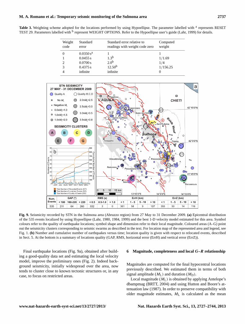
Fig. 9. Seismicity recorded by STN in the Sulmona area (Abruzzo region) from 27 May to 31 December 2009.(a) Epicentral distributionof the 535 events localized by using Hypoellipse (Lahr, 1980, 1984, 1999) and the best 1-D velocity model estimated for this area. Symbolcolours refer to the quality of earthquake locations; symbol shape and dimension refer to their local magnitude. Coloured areas (A–G) pointout the seismicity clusters corresponding to seismic swarms as described in the text. For location map of the represented area and legend, seeFig. 1. (b) Number and cumulative number of earthquakes versus time; location quality is given with respect to relocated events, describedin Sect. 5. At the bottom is a summary of locations quality (GAP, RMS, horizontal error (ErrH) and vertical error (ErrZ)).

Final earthquake locations (Fig. 9a), obtained after build-ing a good-quality data set and estimating the local velocitymodel, improve the preliminary ones (Fig. 2). Indeed back-ground seismicity, initially widespread over the area, nowtends to cluster close to known tectonic structures or, in anycase, to focus on restricted areas.

6 Magnitude, completeness and localG–R relationship

Magnitudes are computed for the final hypocentral locationspreviously described. We estimated them in terms of bothsignal amplitude (ML) and duration (MD).

Local magnitude (ML) is obtained by applying Antelope’sdbampmag (BRTT, 2004) and using Hutton and Boore’s at-tenuation law (1987). In order to preserve compatibility witholder magnitude estimates,ML is calculated as the mean



of the magnitude estimated for each station. The magni-tude is evaluated from the mean of the waveform ampli-tude of the two horizontal components (Bormann, 2002).Single-station compensation coefficients have also been esti-mated and applied. They exhibit randomly distributed valuessmaller than±0.2, except for stations SLA3 and SLA5 (re-spectively+0.42 and+0.30), which were repositioned afterlogistical problems at the original sites.

Local magnitudes, which were estimated in this study,range from−1.5 to 3.7 (Fig. 10a). Of all the events, 93 %haveML between−0.1 and 2, while the remaining 7 % isdistributed as follows: 2 % haveML < −0.1, 4 % haveMLbetween 2 and 3, and only 1 % haveML > 3. Furthermore,8 of 535 earthquakes lack amplitude data due to noise prob-lems.

By comparing ourML estimates to those derived fromISIDE for about 200 events common to both networks(Fig. 10b), it becomes apparent that theML of this study ishigher than that estimated by ISIDE by a value of about 0.15.

As a shortcut to local magnitude estimation, we calculatethe duration magnitude (MD) as well. We used the follow-ing simplified formula according to Havskov and Ottemöller(2010):

MD = a1 + a2 log(τ ), (4)

whereτ is the signal duration in seconds; the distance termis not considered as it turned out to be negligible. Due to thepresence of noise, the signal duration has not been read, andthereforeMD has not been estimated for 207 of 535 events.For the remaining 328 earthquakesMD values range from−0.9 to 3.7.

Mean station coefficients have been estimated by calibrat-ing MD againstML (Fig. 10c) by applying ordinary least-squares and orthogonal regressions. Duration magnitudes arethen obtained by entering the coefficients of the orthogonalregression into the pertinent RESET TEST values of Hypoel-lipse (i.e. (31) equal to−3.2843; (32) equal to 3.3129; (33),(40) and (43) set to 0). It can be seen from Fig. 10c that theorthogonal regression represents the highestML fairly well,even if the data are quite dispersed.

Finally, a statistical analysis of the magnitude versus eventfrequency relationship and an estimation of the completenessmagnitude inferred on the Gutenberg–Richter (1956) modelis carried out by using Zmap software (Wiemer, 2001). Theresult is shown in Fig. 10d. The completeness magnitude(Mc) of our relocated data set (27 May to 31 December 2009)is 1.1. Note that the coefficients of the Gutenberg–Richter re-lationship, i.e. the annuala value (3.49) andb value (0.85),are not representative of the Sulmona Basin only, as part ofthe L’Aquila seismic sequence and a bulk of earthquakes inthe SW Sora region (see Fig. 9a) fall inside the relocatedevents. If we select the events spatially in a buffer zone of20 km around the STN stations, thus selecting earthquakeswhere the detection capabilities of the temporary network are

Fig. 10. (a) Histogram ofML estimates of earthquakes localizedin this study. At the top of the histogram, the percentages of theevents within the corresponding range of magnitude are reported.(b) Histogram of the residuals between local magnitude estimatedin this study and that reported on ISIDE database for coincidentevents.(c) Calibration ofMD magnitude through linear regressionof ML against event duration (τ). In red and blue, the ordinary least-squares and orthogonal regressions, respectively. Dashed lines rep-resent the standard deviation of ordinary least-squares regression.(d) Gutenberg–Richter slope evaluated with 527 events for whichML has been estimated. In blue, the magnitude of completenessMc.



at their best, we obtaina equal to 3.11,b to 0.71 andMc to0.72.

7 Discussion and conclusions

The present paper aims at improving the knowledge of thebackground seismic activity in the Sulmona Basin, an exten-sional active area of the central Apennines known for strongseismic hazard (Pace et al., 2006) but substantially aseismicsince instrumental times (Bagh et al., 2007; Boncio et al.,2009). Thanks to the deployment of a temporary seismic net-work and the analysis of the first seven months of properlyprocessed recorded data, we have obtained a detailed pic-ture of the microseismicity that has not revealed until nowby either existing permanent networks (ISIDE database; DeLuca, 2011) or other similar experiments performed in thepast (Bagh et al., 2007). The meta data gathered during thisperiod were somehow peculiar and time demanding for whatconcerns signal treatment due to the ongoing seismic activityin the L’Aquila area. The processing combines an automaticdetection procedure with operator-assisted selection of win-dows as well as fully manual readings of waveforms on lo-cal events (chosen onS–P time delays). This approach hasproved to be very effective, even though quite time consum-ing, in identifying even very small earthquakes, such as localevents withML < −1 recorded by only one or two stations.The integration of the STN recordings with the data gath-ered by regional and national permanent networks (RSA andRSNC) enriched and strengthened the location quality of thestrongest earthquakes. As phases are homogeneously readand accuracy is clearly stated, a 1-D velocity model of theSulmona area (well constrained within the first 20 km, whichis the maximum depth reached by the quality A earthquakelocations) and a reliableVP /VS ratio of 1.85 were obtained,which guarantees accurate earthquake locations and may beuseful for forthcoming studies in the area.

In this paper, an online catalogue of the analysed earth-quakes is compiled and released as a supplement togetherwith the phase pickings. The catalogue contains the follow-ing: the origin times and the hypocentral coordinates of lo-cated earthquakes; all the parameters useful to establish thequality of their locations (RMS, GAP, number of phasesused, minimum distance, dimension and orientation of er-ror ellipsoids); and the magnitude estimate, with both lo-cal and duration if possible. The catalogue includes 535events, which is about 60 % more than reported in the na-tional ISIDE database. An additional set of 282 not locatedearthquakes is given by phase readings only for possible fur-ther analyses. The quality location of nearly 66 % of thelocated events is A, even though their magnitude is verysmall. Indeed, 99 % of located seismicity is represented byultramicro- (M < 1) and micro-earthquakes (1≤ ML < 3),while only 1 % is represented by small earthquakesML ≥ 3(Hagiwara, 1964) (Fig. 10a). The completeness magnitude

Mc, based on local magnitude estimates, is well constrainedand reaches the value of 1.1 for the whole data set of locatedevents. It decreases to 0.7 if only the area strictly pertain-ing to the STN stations is considered. This low value ofMcconfirms that the adopted semi-automatic procedure basedon automatic detection of events and manual picking is veryeffective for investigating the microseismicity.

A well-constrainedG–R slope was estimated from the mi-croseismic data (Fig. 10d). We observe that the productivityrates shown by thea value are nearly constant if normal-ized to the area outlined by the temporary stations’ cover-age, whereas theb value decreases from 0.85 to 0.71. Nev-ertheless, the shortness of the time interval investigated andthe limitations in the data sample do not allow for interpret-ing these lowb values as a stress indicator (see, for exam-ple, Gulia and Wiemer, 2010). In the Sulmona area, station-ary background conditions might have been influenced bystatic/dynamic stress changes induced by the main L’Aquilaearthquakes. Evidence of stress loading in the Sulmona basi-nal area induced not only by the L’Aquila 2009 earthquakein the north but also by the 1984 Val di Sangro earthquake inthe south was pointed out by De Natale et al. (2011) based onthe results from coseismic Coulomb stress change studies.

A seismotectonic analysis of the geometric and kinematicrelationship between the Sulmona microearthquake activityand the active faults in the area are beyond the scope of thispaper. Nevertheless, some preliminary observations on thespace–time distribution of identified clusters of seismic activ-ity and on the overall seismogenic thickness can be advanced.We observe that the background seismicity is not uniformlydistributed in the study area but rather clustered in specificzones, mainly close to known active faults (Fig. 9a). Pre-vailing activity is observed in the northwestern corner of thestudy area, which coincides with the southern end of the Pa-ganica seismogenic source responsible for the 2009 L’Aquilaearthquake (Mw = 6.3, Lavecchia et al., 2012); conversely,the area of the Sulmona Plain remained almost completelyaseismic during the whole of the observation time.

The temporal evolution of the recorded seismic activity,schematized as a cumulative number of events versus time(Fig. 9b), shows a sharp decrease in seismic rate at the end ofJune, e.g. after nearly one month of registration and nearlytwo months after the 6 April 2009 earthquake (Mw = 6.3).The remaining portion of the cumulative slopes shows otherjumps, corresponding to local and short-lasting increases inthe seismic activity. Three swarms were recorded from 2 to22 June. They occurred within the hanging wall of the Por-rara Fault (cluster A, withML up to 1.7, and C1, withMLup to 2.5 in Fig. 9a), and within the footwall of the MorroneFault (cluster B, withML up to 1.2, and C2 withML up to 0.9in Fig. 9a). Specifically, the swarms are placed at southernand northern tips of the Morrone-Porrara extensional align-ment.



On 4 August the area near Roccasicura (Molise region), lo-cated along the SSE-ward direction of the Morrone–Porraraextensional alignment, was affected by a small swarm of 10earthquakes (cluster D in Fig. 9a) at depths between 13 and17 km, with two larger events ofML = 3.5 and 3.6 (Fig. 9a).Two other swarms occurred at the beginning of October2009. The first one (12 events between 4 and 5 October, withML up to 1.7; cluster E in Fig. 9a) was located at the hangingwall of the Marsicano Fault at depths of 6–12 km; the secondone (80 events between 6 and 8 October, withML up to 3.6 asin ISIDE; cluster F in Fig. 9a) nucleated near Sora (Lazio re-gion) at a depth of 6 to 14 km. Finally, on 19 and 20 Novem-ber, another increase of seismicity, with spatial distributionsimilar to that of the late June activity, was recorded at thefootwall of the Morrone Fault (cluster G1 withML up to 1.6in Fig. 9a) and at the hanging wall of the Porrara Fault (clus-ter G2 withML up to 2.9 in Fig. 9a).

We also performed a preliminarily evaluation on the Sul-mona seismogenic layer, defined as the depth layer that re-leases the largest number of earthquakes (i.e. 95 % of theseismicity – D95; Williams, 1996; Fernandez-Ibañez andSoto, 2008). The frequency–depth histogram of Fig. 8i,which was only built on the basis of quality A earthquakes,shows that 7 % of the events were shallower than 5 km, 24 %occurred at depths between 5 and 9 km, 42 % were concen-trated in the 9–12 km depth interval, 22 % were between 12and 17 km, and the remaining 5 % between 17 and 21 km.Therefore, the base of the seismogenic layer, which releases95 % of the seismicity, is located at a depth of 17 km. A thick-ness of 12 km (from 5 to 17 km) may be assumed for the brit-tle layer, which is considered as the layer within which nearly90 % of the seismicity occurs. These values are in agreementwith other independent estimates done in this sector of theApennines based on rheological evaluations (Boncio et al.,2009).

In conclusion, we point out that the detailed analysis andthe quality study performed in this paper in order to obtaina low-magnitude complete catalogue for the Sulmona areaconfirm and further highlight the low seismicity rate charac-terizing the study area, with important implications in seis-mic hazard evaluation.

Appendix A

Phase reading uncertainties

Uncertainty in phase readings is rarely declared in earth-quake locations and catalogues, but this is an important el-ement because location codes use this information in theirweighting schemes. Formally, the estimate of measurementerror has to be evaluated from a probabilistic point of view.According to this, the onset of a seismic phase should be de-scribed by a probabilistic function that reaches its maximumexactly at the arrival time of this phase, and the standard error

Table A1. Weighting scheme adopted in the preliminary locationsperformed by using Hypo71 (Lee and Lahr, 1975).

WeightCode

ReadingError

01234

< 0.01 s[0.01 s–0.04 s)[0.04 s–0.20 s)[0.20 s–1.00 s)≥ 1.00 s

corresponds to the standard deviation of the population. Inthis way information on statistical properties of the errorscould be retrieved. More often, only a qualitative evaluationof the reading error is available, and the operator’s choicecannot be evaluated rigorously. Reading errors are detectedby a change in the amplitude and in the frequency contentof the seismic signal, and they are usually represented by atime window whose width is estimated by the operator anddepends on the signal-to-noise ratio and the dominant fre-quency of the arriving phase (Husen and Hardebeck, 2010).Phase reading errors are then classified into categories whichcorrespond to weight codes that are directly used by locationalgorithms. The larger the reading uncertainty, the higher theweight code is and the less this reading influences earthquakelocation. The mapping of reading errors into weights may becontrolled by the seismologist, even though this is not alwaysdeclared. For our preliminary earthquake locations, given inFig. 2 in the main text, the setting of weighting scheme tunedfor performing locations with Hypo71 is shown in Table A1.

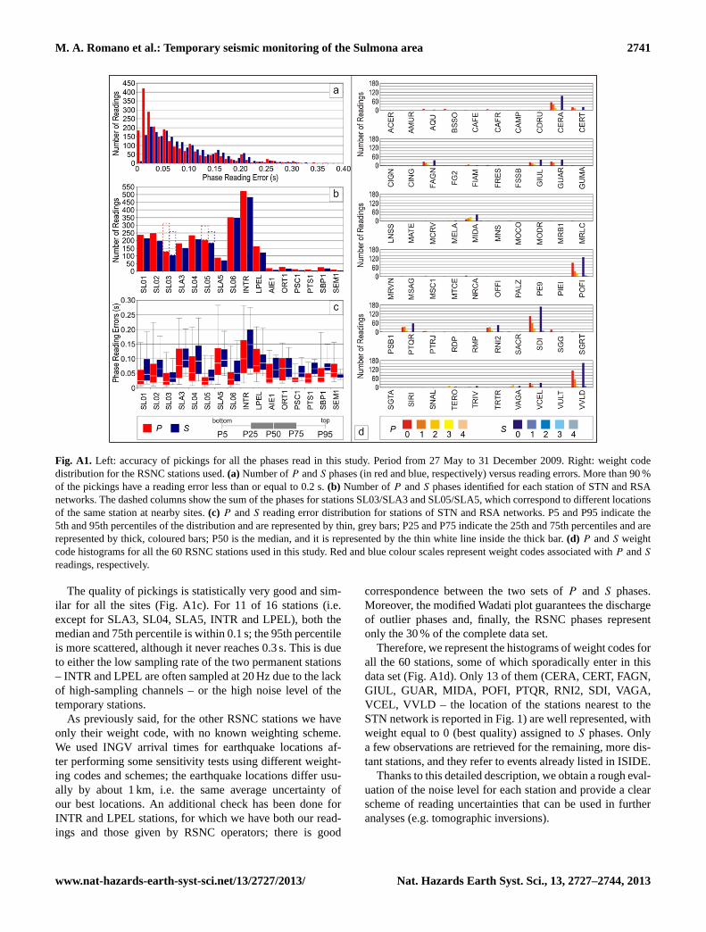
Some histograms of the phase reading errors are given inFig. A1. The data set contains readings from the STN andRSA networks obtained for this study manually, whereas wecannot retrieve the reading uncertainties for all the phasesprovided by the RSNC network, for which only the weightcode and polarities, if any, are given. More than 90 % of theP and S original phases have a reading error less than orequal to 0.2 s (see Fig. A1a), while a few outliers (seven forP phases, one forS phases), not represented in Fig. A1a,are in the range 0.4–0.54 s. Thus, none of our picks is givenweight 4.

The permanent INTR station (see its location in Fig. 1)is the site with the greatest number of readings (Fig. A1b)related to local events. Also, sites SL03/SLA3, SL05/SLA5and SL06 are well represented (about or more than 300P ’s).Three stations (i.e. SL01, SL04 and LPEL) have less data be-cause of some instrumental acquisition problems (for details,see de Nardis et al., 2011). Conversely, the small number ofreadings on the RSA stations is probably due to the triggered-mode acquisition, which cut off the detected earthquakes ata higher threshold.



Fig. A1. Left: accuracy of pickings for all the phases read in this study. Period from 27 May to 31 December 2009. Right: weight codedistribution for the RSNC stations used.(a) Number ofP andS phases (in red and blue, respectively) versus reading errors. More than 90 %of the pickings have a reading error less than or equal to 0.2 s.(b) Number ofP andS phases identified for each station of STN and RSAnetworks. The dashed columns show the sum of the phases for stations SL03/SLA3 and SL05/SLA5, which correspond to different locationsof the same station at nearby sites.(c) P andS reading error distribution for stations of STN and RSA networks. P5 and P95 indicate the5th and 95th percentiles of the distribution and are represented by thin, grey bars; P25 and P75 indicate the 25th and 75th percentiles and arerepresented by thick, coloured bars; P50 is the median, and it is represented by the thin white line inside the thick bar.(d) P andS weightcode histograms for all the 60 RSNC stations used in this study. Red and blue colour scales represent weight codes associated withP andS

readings, respectively.

The quality of pickings is statistically very good and sim-ilar for all the sites (Fig. A1c). For 11 of 16 stations (i.e.except for SLA3, SL04, SLA5, INTR and LPEL), both themedian and 75th percentile is within 0.1 s; the 95th percentileis more scattered, although it never reaches 0.3 s. This is dueto either the low sampling rate of the two permanent stations– INTR and LPEL are often sampled at 20 Hz due to the lackof high-sampling channels – or the high noise level of thetemporary stations.

As previously said, for the other RSNC stations we haveonly their weight code, with no known weighting scheme.We used INGV arrival times for earthquake locations af-ter performing some sensitivity tests using different weight-ing codes and schemes; the earthquake locations differ usu-ally by about 1 km, i.e. the same average uncertainty ofour best locations. An additional check has been done forINTR and LPEL stations, for which we have both our read-ings and those given by RSNC operators; there is good

correspondence between the two sets ofP and S phases.Moreover, the modified Wadati plot guarantees the dischargeof outlier phases and, finally, the RSNC phases representonly the 30 % of the complete data set.

Therefore, we represent the histograms of weight codes forall the 60 stations, some of which sporadically enter in thisdata set (Fig. A1d). Only 13 of them (CERA, CERT, FAGN,GIUL, GUAR, MIDA, POFI, PTQR, RNI2, SDI, VAGA,VCEL, VVLD – the location of the stations nearest to theSTN network is reported in Fig. 1) are well represented, withweight equal to 0 (best quality) assigned toS phases. Onlya few observations are retrieved for the remaining, more dis-tant stations, and they refer to events already listed in ISIDE.

Thanks to this detailed description, we obtain a rough eval-uation of the noise level for each station and provide a clearscheme of reading uncertainties that can be used in furtheranalyses (e.g. tomographic inversions).



Supplementary material related to this article isavailable online athttp://www.nat-hazards-earth-syst-sci.net/13/2727/2013/nhess-13-2727-2013-supplement.zip.

Acknowledgements.This project is self-financed by OGS (CRSDepartment) and the University of Chieti (GeosisLab, headedby Giusy Lavecchia). We thank all mayors of the municipalitiesinvolved, Silvano Agostini of the regional board of the Ministry ofCultural Heritage and Environmental Conservation, and the DPC(Civil Protection Department) and the INGV (National Institute ofGeophysics and Volcanology) for data exchange. Special thanks goto Gaetano De Luca (INGV) for his great work done in gatheringand providing us with the data recorded by the Abruzzo SeismicNetwork (RSA), and also to Francesco Mele (INGV) for his pre-cious help in retrieving the phase picking of the National SeismicNetwork (RSNC). We also thank the Editor Stefano Tinti and thereviewers Dario Albarello, Elena Eva and the anonymous one forthe constructive remarks that improve the original manuscript.

Edited by: S. TintiReviewed by: D. Albarello, E. Eva, and one anonymous referee

References

Bagh, S., Chiaraluce, L., De Gori, P., Moretti, M., Govoni, A.,Chiarabba, C., Di Bartolomeo, P., and Romanelli, M.: Back-ground seismicity in the Central Apennines of Italy: TheAbruzzo region case study, Tectonophysics, 444, 80–92, 2007.

Barchi, M., Minelli, G., Magnani, B., and Mazzotti, A.: Line CROP03: Northern Apennines, Memorie Descrittive della Carta Geo-logica d’Italia, LXII, 127–136, 2003.

Boncio, P., Lavecchia, G., and Pace, B.: Defining a model of 3Dseismogenic sources for Seismic Hazard Assessment applica-tions: The case of Central Apennines (Italy), J. Seismol, 8, 407–425, 2004.

Boncio, P., Tinari, D. P., Lavecchia, G., Visini, F., and Milana,G.: The instrumental seismicity of the Abruzzo Region in Cen-tral Italy (1981–2003): Seismotectonic Implications, Italian Jour-nal of Geosciences (Bollettino della Società Geologica Italiana),128, 367–380, 2009.

Bondar, I.: Hypocentre determination of local earthquakes using ge-netic algorithm, Acta Geodaetica Geophysica Hungarica, 29, 39–56, 1994.

Bormann, P.: New Manual of Seismological Observatory Practice,GeoForschungsZentrum Potsdam, 2002.

BRTT (Boulder Real Time Technology): Evolution of the Commer-cial ANTELOPE Software, Open file Report, available at:http://www.brtt.com/docs/evolution.pdf(last access: 22 April 2013),2004.

Castello, B., Selvaggi, G., Chiarabba, C., and Amato, A.: CSI – Cat-alogo della sismicità italiana 1981–2002, versione 1.1, INGV-CNT, Roma, available at:http://csi.rm.ingv.it/(last access: 22April 2013), 2006.

Ceccaroni, E., Ameri, G., Gómez Capera, A. A., and GaladiniF.: The 2nd century AD earthquake in Central Italy: archaeo-

seismological data and seismotectonic implications, Nat. Haz-ards, 50, 335–359, doi:10.1007/s11069-009-9343-x, 2009.

Chatelain, J.: Étude fine de la sismicité en zone de collisioncontinentale à l’aide d’un réseau de stations portables: la ré-gion Hindu–Kush–Pamir, Ph.D. thesis, Université Paul Sabatier,Toulouse, 1978.

Chiarabba, C., Jovane, L., and Di Stefano, R.: A new look to the Ital-ian seismicity: seismotectonic inference, Tectonophysics, 395,251–268, 2005.

Chiarabba, C., Amato, A., Anselmi, M., Baccheschi, P., Bianchi,I., Cattaneo, M., Cecere, G., Chiaraluce, L., Ciaccio, M. G., DeGori, P., De Luca, G., Di Bona, M., Di Stefano, R., Faenza, L.,Govoni, A., Improta, L., Lucente, F. P., Marchetti, A., Margher-iti, L., Mele, F., Michelini, A., Monachesi, G., Moretti, M., Pas-tori, M., Piana Agostinetti, N., Piccinini, D., Roselli, P., Seccia,D., and Valoroso, L.: The 2009 L’Aquila (central Italy) MW6.3earthquake: Main shock and aftershocks, Geophys. Res. Lett.,36, L18308, doi:10.1029/2009GL039627, 2009.

Chiarabba, C., Bagh, S., Bianchi, I., De Gori, P., and Barchi, M.:Deep structural heterogeneities and the tectonic evolution of theAbruzzi region (Central Apennines, Italy) revealed by microseis-micity, seismic tomography, and teleseismic receiver functions,Earth Planet. Sci. Lett., 295, 462–476, 2010.

Chiaraluce, L., Chiarabba, C., De Gori, P., Di Stefano, R., Improta,L., Piccinini, D., Schlagenhauf, A., Traversa, P., Valoroso, L.,and Voisin, C.: The 2009 L’Aquila (central Italy) seismic se-quence, Bollettino di Geofisica Teorica ed Applicata, 52, 367–387, doi:10.4430/bgta0019, 2011.

Christensen, N. I. and Mooney, W. D.: Seismic velocity structureand composition of the continental crust: A global view, J. Geo-phys. Res., 100, 9761–9788, 1995.

De Luca, G.: La Rete Sismica regionale Abruzzo e sua inte-grazione con la RSN, in: Riassunti estesi del I Workshop Tecnico“Monitoraggio sismico del territorio nazionale: stato dell’arte esviluppo delle reti di monitoraggio sismico”, INGV, Roma, 22–23, 2011.

De Luca, G., Scarpa, R., Filippi, L., Gorini, A., Marcucci, S.,Marsan, P., Milana, G., and Zambonelli, E.: A detailed analysisof two seismic sequences in Abruzzo, Central Apennines, Italy,J. Seismol., 4, 1–21, 2000.

de Nardis, R., Garbin, M., Lavecchia, G., Pace, B., Peruzza, L., Pri-olo, E., Romanelli, M., Romano, M. A., Visini, F., and Vuan, A.:A temporary seismic monitoring of the Sulmona area (Abruzzo,Italy) for seismotectonic purposes, Bollettino di Geofisica Teor-ica ed Applicata, 52, 651–666, 2011.

De Natale, G., Crippa, B., Troise, C., and Pingue, F.: Abruzzo,Italy, Earthquakes of April 2009: Heterogeneous Fault-Slip Mod-els and Stress Transfer from Accurate Inversion of ENVISAT-InSAR Data, Bull. Seismol. Soc. Am., 101, 2340–2354,doi:10.1785/0120100220, 2011.

Di Luzio, E., Mele, G., Tiberti, M. M., Cavinato, G. P., and Parotto,M.: Moho deepening and shallow upper crustal delamination be-neath the central Apennines, Earth Planet. Sci. Lett., 280, 1–12,2009.

Elter, F. M., Elter, P., Eva, C., Eva, E., Kraus, R. K., Padovano, M.,and Solarino, S.: An alternative model for the recent evolution ofthe Northern-Central Apennines (Italy), J. Geodynam., 54, 55–63, 2012.


http://www.nat-hazards-earth-syst-sci.net/13/2727/2013/nhess-13-2727-2013-supplement.zip

http://www.nat-hazards-earth-syst-sci.net/13/2727/2013/nhess-13-2727-2013-supplement.zip

http://www.brtt.com/docs/evolution.pdf

http://www.brtt.com/docs/evolution.pdf

http://csi.rm.ingv.it/

http://dx.doi.org/10.1007/s11069-009-9343-x

http://dx.doi.org/10.1029/2009GL039627

http://dx.doi.org/10.4430/bgta0019

http://dx.doi.org/10.1785/0120100220


Fernandez-Ibañez, F. and Soto, J. I.: Crustal rheology and seismicityin the Gibraltar Arc (western Mediterranean), Tectonics, 27, 1–18, 2008.

Galadini, F. and Messina, P.: Early-Middle Pleistocene eastward mi-gration of the Abruzzi Apennine (central Italy) extensional do-main, J. Geodynam, 37, 57-81, 2004.

Galli, P., Galadini, F., and Pantosti, D.: Twenty years of paleoseis-mology in Italy, Earth-Sci. Rev., 88, 89–117, 2008.

Garbin, M. and Priolo, E.: Seismic event recognition in the Trentinoarea (Italy): performance analysis of a new semi-automatic sys-tem, Seismol. Res. Lett., 84, 65–74, doi:10.1785/0220120025,2013.

Ghisetti, F. and Vezzani, L.: Normal faulting, extension and upliftin the outer thrust belt of the central Apennines (Italy): role ofthe Caramanico fault, Basin Res., 14, 225–236, 2002.

Gori, S., Giaccio, B., Galadini, F., Falcucci, E., Messina, P.,Sposato, A., and Dramis, F.: Active normal faulting along the Mt.Morrone south-western slopes (central Apennines, Italy), Int. J.Earth Sci., 100, 157–171, 2011.

Guidoboni, E., Ferrari, G., Mariotti, D., Comastri, A., Tarabusi, G.,and Valensise, G.: CFTI4Med, Catalogue of Strong Earthquakesin Italy (461 B.C.–1997) and Mediterranean Area (760 B.C.–1500), available at:http://storing.ingv.it/cfti4med/(last access:22 April 2013), 2007.

Gulia, L. and Wiemer, S.: The influence of tectonic regimes on theearthquake size distribution: A case study for Italy, Geophys.Res. Lett., 37, L10305, doi:10.1029/2010GL043066, 2010.

Gutenberg, B. and Richter, C. F.: Earthquake magnitude, inten-sity, energy, and acceleration (second paper), Bull. Seismol. Soc.Am., 46, 138–154, 1956.

Hagiwara, T.: Brief description of the project proposed by the earth-quake prediction research group of Japan, in: Proc. US – JapanConf. Res. Relat. Earthquake Prediction Probl., Earthquake Re-search Institute, Tokyo, 10–12, 1964.

Havskov, J. and Ottemöller, L.: Routine Data Processing in Earth-quake Seismology, xi+ 347 pp., Springer, ISBN 978-90-481-8696-9, 2010.

Husen, S. and Hardebeck, J. L.: Earthquake location accuracy,Community Online Resource for Statistical Seismicity Analysis,doi:10.5078/corssa-55815573, available at:http://www.corssa.org (last access: 22 April 2013), 2010.

Hutton, L. K. and Boore, D. M.: The ML scale in Southern Califor-nia, Bull. Seismol. Soc. Am., 77, 2074–2094, 1987.

ISIDE Working Group (INGV): Italian Seismological Instrumen-tal and parametric database, available at:http://iside.rm.ingv.it/iside/standard/index.jsp(last access: 22 February 2012), 2010.

ISB Working Group (INGV): Italian Seismic Bulletin, availableat: http://bollettinosismico.rm.ingv.it/, last access: 22 February2012.

Kissling, E., Ellsworth, W. L., Eberhart-Phillips, D., and Kradolfer,U.: Initial reference models in local earthquake tomography, J.Geophys. Res., 99, 19635–19646, 1994.

Lahr, J. C.: HYPOELLIPSE/MULTICS: A Computer Program forDetermining Local Earthquake Hypocentral Parameters, Magni-tude and First-Motion Pattern, US Geological Survey Open-FileReport 80-59, 59 pp., 1980.

Lahr, J. C.: HYPOELLIPSE/VAX: A Computer Program for De-termining Local Earthquake Hypocentral Parameters, Magnitude

and First-Motion Pattern, US Geological Survey Open-File Re-port 84-519, 76 pp., 1984.

Lahr, J. C.: HYPOELLIPSE: A Computer Program for DeterminingLocal Earthquake Hypocentral Parameters, Magnitude and First-Motion Pattern (Y2K Compliant Version), Version 1.0., US Geo-logical Survey Open-File Report 99-23, On-Line Edition, 1999.

Lavecchia, G. and de Nardis, R.: Seismogenic sources of majorearthquakes of the Maiella area (Central Italy): constraints frommacroseismic field simultaions and regional seimotectonics, UR4.01-S1-29, Poster at the INGV-DPC meeting, Rome, November,2009.

Lavecchia, G., Ferrarini, F., Brozzetti, F., de Nardis, R., Bon-cio, P., and Chiaraluce, L.: From surface geology to after-shock analysis: Constraints on the geometry of the L’Aquila2009 seismogenic fault system, Italian J. Geosci., 131, 330–347,doi:10.3301/IJG.2012.24, 2012.

Lee, W. H. K. and Lahr, J. C.: HYP071 (Revised): A Computer Pro-gram for Determining Hypocenter, Magnitude and First-motionPattern of Local Earthquakes, US Geological Survey Open FileReport 75-311, 1975.

Lee, W. H. K. and Stewart, S. W.: Principles and Applications ofMicroearthquake Networks, Academic Press, New York, 293 pp.,1981.

Lomax, A.: SeisGram2K (5.3), Mouans-Sartoux, available at:http://alomax.free.fr/seisgram/SeisGram2K.html(last access: 22 April2013), 2008.

Margheriti, L., Chiaraluce, L., Voisin, C., Cultrera, G., Govoni,A., Moretti, M., Bordoni, P., Luzi, L., Azzara, R., Valoroso,L., Di Stefano, R., Mariscal, A., Improta, L., Pacor, F., Milana,G., Mucciarelli, M., Parolai, S., Amato, A., Chiarabba, C., DeGori, P., Lucente, F. P., Di Bona, M., Pignone, M., Cecere, G.,Criscuoli, F., Delladio, A., Lauciani, V., Mazza, S., Di Giulio,G., Cara, F., Augliera, P., Massa, M., D’Alema, E., Marzorati, S.,Sobiesiak, M., Strollo, A., Duval, A. M., Dominique, P., Delouis,B., Paul, A., Husen, S., and Selvaggi, G.: Rapid response seismicnetworks in Europe: lessons learnt from the L’Aquila earthquakeemergency, Ann. Geophys., 54, 392–399, doi:10.4401/ag-4953,2011.

Pace, B., Peruzza, L., Lavecchia, G., and Boncio, P.: Layered Seis-mogenic Source Model and Probabilistic Seismic-Hazard Analy-ses in Central Italy, Bull. Seismol. Soc. Am., 96, 107–132, 2006.

Patacca, E., Scandone, P., Di Luzio, E., Cavinato, G. P., andParotto, M.: Structural architecture of the central Apennines:interpretation of the CROP 11 seismic profile from the Adri-atic coast to the orographic divide, Tectonics, 27, TC3006,doi:10.1029/2005TC001917, 2008.

Peruzza, L., Pace, B., and Visini, F.: Fault-Based EarthquakeRupture Forecast in Central Italy: Remarks after the L’AquilaMw 6.3 Event, Bull. Seismol. Soc. Am., 101, 404–412,doi:10.1785/0120090276, 2011.

Rovida, A., Camassi, R., Gasperini, P., and Stucchi, M. (Eds.):CPTI11, la versione 2011 del Catalogo Parametrico dei Terre-moti Italiani, Milano, Bologna, available at:http://emidius.mi.ingv.it/CPTI11/(last access: 22 April 2013), 2011.

Scarascia, S., Lozej, A., and Cassinis, R.: Crustal structures of theLigurian, Tyrrhenian and Ionian seas and adjacent onshore areasinterpreted from wide angle seismic profiles, Bollettino di Ge-ofisica Teorica ed Applicata, 36, 5–19, 1994.


http://dx.doi.org/10.1785/0220120025

http://storing.ingv.it/cfti4med/

http://dx.doi.org/10.1029/2010GL043066

http://dx.doi.org/10.5078/corssa-55815573

http://www.corssa.org

http://www.corssa.org



http://bollettinosismico.rm.ingv.it/

http://dx.doi.org/10.3301/IJG.2012.24

http://alomax.free.fr/seisgram/SeisGram2K.html

http://alomax.free.fr/seisgram/SeisGram2K.html

http://dx.doi.org/10.4401/ag-4953

http://dx.doi.org/10.1029/2005TC001917

http://dx.doi.org/10.1785/0120090276

http://emidius.mi.ingv.it/CPTI11/

http://emidius.mi.ingv.it/CPTI11/


Trippetta, F., Collettini, C., Barchi, M. R., Lupattelli, A., andMirabella, F.: A multidisciplinary study of a natural example ofCO2 geological storage in central Italy, Int. J. Greenhouse GasControl, 12, 72–83, 2013.

Wiemer, S.: A Software Package to Analyze Seismicity: ZMAP,Seismol. Res. Lett., 72, 373–382, available at:http://www.earthquake.ethz.ch/software/zmap(last access: 22 April 2013),2001.

Williams, C. F.: Temperature and the seismic/aseismic transition:Observations from the 1992 Landers earthquake, Geophys. Res.Lett., 23, 2029–2032, 1996.

Working Group OASIS – The OGS Archive System of InstrumentalSeismology, available at:http://oasis.crs.inogs.it(last access: 22April 2013), 2011.


http://www.earthquake.ethz.ch/software/zmap

http://www.earthquake.ethz.ch/software/zmap

http://oasis.crs.inogs.it

Documents

Temporary seismic monitoring of the Sulmona area (Abruzzo, Italy