Tegoeh Tjahjowidodo Characterization, Modelling and Control of Mechanical Systems Comprising Material and Geometrical Nonlinearities Tegoeh Tjahjowidodo

W

P M A

Tegoeh Tjahjowidodo

Characterization, Modelling and Control of Mechanical Systems Comprising Material and

Geometrical Nonlinearities

Tegoeh Tjahjowidodo

Katholieke Universiteit Leuven

Departement Werktuigkunde, Div. PMA

Thursday 16 November 2006

Doctoral Defence

Tegoeh Tjahjowidodo

P M A

W

Overview

Introduction– Nonlinearity sources– Dynamic signal classification

Geometric Nonlinearity (Backlash)

Material Nonlinearity (Friction)

Control of Nonlinear Systems

Application on a Real SystemMechanical Systems

with Harmonic Drive elements

Conclusions







Conclusions

Introduction Introduction– Nonlinearity sources– Dynamic signal classification






Conclusions

Geometric Nonlinearity







Conclusions

Material Nonlinearity







Conclusions








Conclusions

Application on Real System







Conclusions

Conclusions

Tegoeh Tjahjowidodo

P M A

W

Introduction

Motivation:

Having better understanding of a system via appropriate techniques

System Identification !

Introduction





ConclusionsThere is no general identification method applicable to all systems.

this depends on the characteristic of the system and the type of the signal involved in the identification.

Identification purposes:– Dynamic behaviour analysis– Design engineering– Damage detection– Control design– Control design

Tegoeh Tjahjowidodo

P M A

W

Characteristic of systems

prescribed displacement (û)

displacement (u)

strain(e)

stress(σ)

body force(b)

prescribed forces(t)

Force B.C

Displacement B.C.

Material nonlinearity

Geometric nonlinearity

Nonlinearity in a mechanical system can be attributed to different sources:

Introduction





Conclusions

Tegoeh Tjahjowidodo

P M A

W

Geometrical and Material Nonlinearities

Geometric Nonlinearity– the change in geometry as the structure deforms causes a

nonlinear change of the parameters in the system

hardening spring, softening spring, saturation, …

Material Nonlinearity– the behaviour of material depends on the current

deformation

frictional losses, ferromagnetism

Introduction





Conclusions

Tegoeh Tjahjowidodo

P M A

W

Dynamic Signal Classification

Chaotic:• Lyapunov Exponent• Correlation Dimension• etc

‘Well-behaved’

Deterministic

Dynamic Signal

Random

Stationary:•Frequency Response Function

•Volterra•etc

Non-stationary:•Short Time Fourier Transform

•Wigner-Ville•Wavelet•Hilbert

In general dynamic signals can be classified:

Introduction





Conclusions

Tegoeh Tjahjowidodo

P M A

W


Tegoeh Tjahjowidodo

P M A

W


Case study:mechanical system with backlash element

Backlash:

In a mechanical system, any lost motion between driving and driven elements due to clearance between parts.

ck1

k0

x0 x

m

Fin

k1

k1+ k0

x0

-x0

x

k1x+

F(x

)

Introduction


• Well-behaved

• Chaotic




Conclusions

Tegoeh Tjahjowidodo

P M A

W

Backlash

Two different cases might appear:Introduction


• Well-behaved

• Chaotic




Conclusions

– ‘well-behaved’ response for periodic input• Skeleton identification

– Hilbert transform

– Wavelet analysis

– chaotic response for periodic input• Chaos quantification

– Lyapunov exponent

• Surrogate Data Test

Tegoeh Tjahjowidodo

P M A

W

Skeleton identification

Free vibration response can be represented in the combination of envelope and instantaneous phase.

SDOF system: 0y)A(y)A(h2y 200

Introduction


• Well-behaved

• Chaotic




Conclusions

y(t) = A(t)·cos [(t)-

Tegoeh Tjahjowidodo

P M A

W

Skeleton identification

Envelope and instantaneous phase of the free vibration response can be used as a

mechanical signature of the dynamic parameters of the system (Feldman 1994a).

Introduction


• Well-behaved

• Chaotic




Conclusions

Tegoeh Tjahjowidodo

P M A

W

Skeleton signature examples (1)

Signatures of restoring forces

Introduction


• Well-behaved

• Chaotic




Conclusions

Tegoeh Tjahjowidodo

P M A

W

Skeleton signature examples (2)

Signatures of damping forces

Introduction


• Well-behaved

• Chaotic




Conclusions

Tegoeh Tjahjowidodo

P M A

W

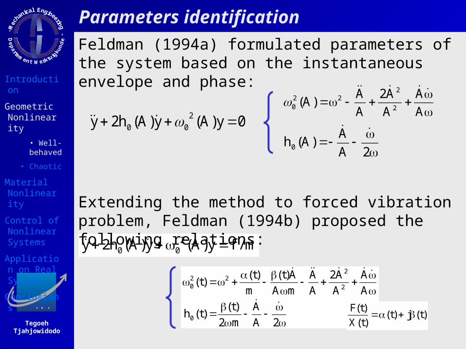
Parameters identification

Feldman (1994a) formulated parameters of the system based on the instantaneous envelope and phase:

0y)A(y)A(h2y 2

00

22 20 2

0

(t) (t)A A 2A A(t)

m A m A A A

(t) Ah (t)

2 m A 2

20 0y 2h (A)y (A)y f / m

Extending the method to forced vibration problem, Feldman (1994b) proposed the following relations:

F(t)(t) j (t)

X(t)

A

A

A

A2

A

A)A(

2

222

0

2A

A)A(h 0

Introduction


• Well-behaved

• Chaotic




Conclusions

Tegoeh Tjahjowidodo

P M A

W

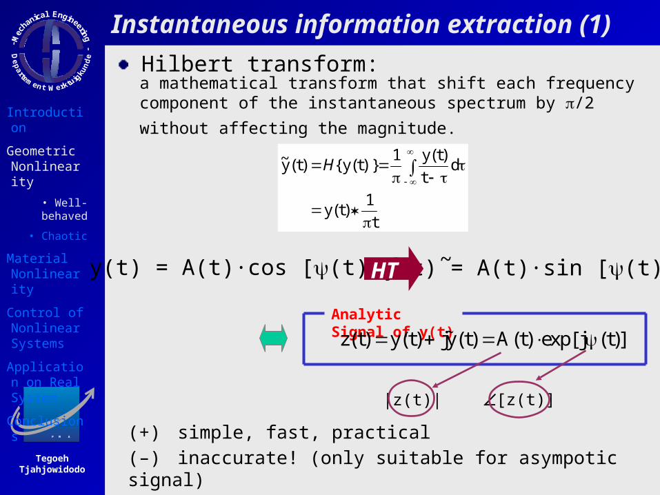
Instantaneous information extraction (1)

Hilbert transform:a mathematical transform that shift each frequency component of the

instantaneous spectrum by /2 without affecting the magnitude.

t

1)t(y

dt

)t(y1)}t(y{)t(y~

H

y(t) = A(t)·cos [(t)-

Analytic Signal of y(t)

z(t) y(t) jy(t) A(t) exp[ j (t)]

(+) simple, fast, practical

|z(t)| [z(t)]

y(t) = A(t)·sin [(t)-HT ~

(–) inaccurate! (only suitable for asympotic signal)

Introduction


• Well-behaved

• Chaotic




Conclusions

Tegoeh Tjahjowidodo

P M A

W

Instantaneous information extraction (2)

Wavelet transform:

dts

t)t(x

s),s(W

1

a time-frequency representation (TFR) technique

(Complex Morlet Wavelet)

b2

c f/ttjb eef)t(

(+) accurate!(–) time consuming, error at the edges, cumbersome

instantaneous frequency(in dilation form):

)τ(

)0(s c

envelope in modulus of wavelet:

))τ(s()(As

),s(W * 1

Introduction


• Well-behaved

• Chaotic




Conclusions

Tegoeh Tjahjowidodo

P M A

W

Illustration of extraction

Damped-chirp signal

Envelope Estimation

0 2 4 6 8 10-1

-0.5

0

0.5

1

1.5

time (s)

Am

plit

ud

e

HT techniqueWavelet technique

Instantaneous Frequency Estimation

0 2 4 6 8 10-10

-5

0

5

10

15

20

time (s)F

req

ue

ncy

HT techniqueWavelet technique

Introduction


• Well-behaved

• Chaotic




Conclusions

Tegoeh Tjahjowidodo

P M A

W

Experimental Setup

Encoder #2

2nd link

1st linkEncoder #1

Schematic drawing of a two-link mechanism

• 1st link fixed

• backlash was introduced in the joint

• considered as a base motion system

Introduction


• Well-behaved

• Chaotic




Conclusions

Tegoeh Tjahjowidodo

P M A

W

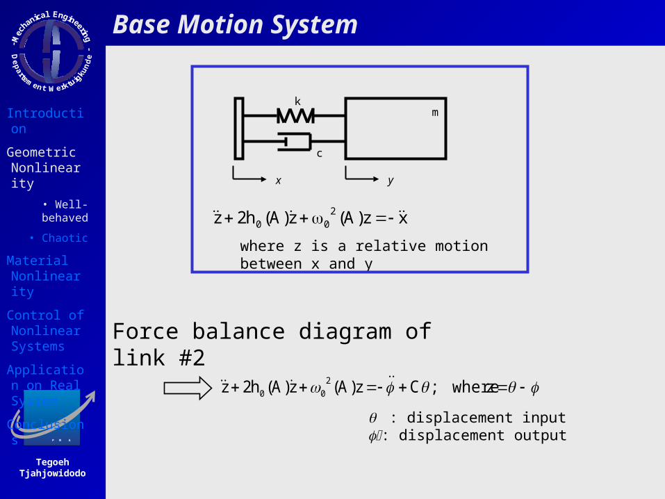
Base Motion System

Force balance diagram of link #2

z where;Cz)A(z)A(h2z 2

00

Introduction


• Well-behaved

• Chaotic




Conclusions

xz)A(z)A(h2z 200

where z is a relative motion between x and y

k

c

m

x y

: displacement input: displacement output

Tegoeh Tjahjowidodo

P M A

W

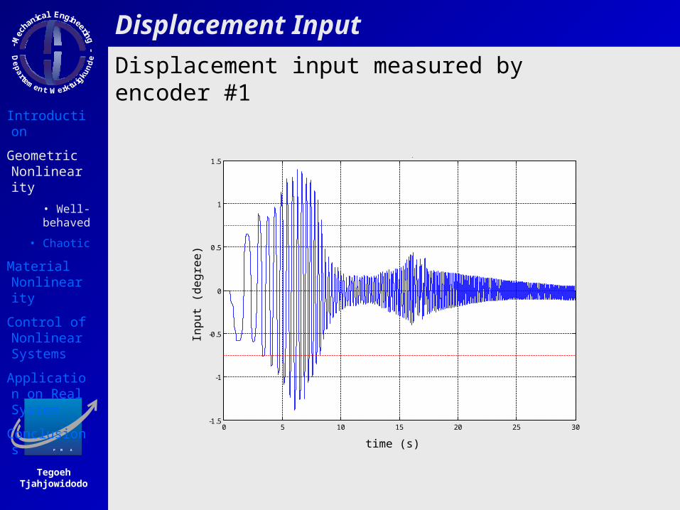
Displacement Input

Displacement input measured by encoder #1

0 5 10 15 20 25 30-1.5

-1

-0.5

0

0.5

1

1.5

time (s)

Inp

ut

(de

gre

e)

Input side displacement(encoder input)

Inp

ut

(de

gre

e)

time (s)

Introduction


• Well-behaved

• Chaotic




Conclusions

Tegoeh Tjahjowidodo

P M A

W

Displacement Output

Displacement output measured by encoder #2

0 5 10 15 20 25 30-2.5

-2

-1.5

-1

-0.5

0

0.5

1

1.5

2

2.5

time (s)

Ou

tpu

t (d

eg

ree

)

Output side displacement(encoder output)

Ou

tpu

t (d

eg

ree

)

time (s)

Introduction


• Well-behaved

• Chaotic




Conclusions

Tegoeh Tjahjowidodo

P M A

W

Relative Motion

Relative motion between output and input ()

0 5 10 15 20 25 30-1

-0.8

-0.6

-0.4

-0.2

0

0.2

0.4

0.6

0.8

1

time (s)

Re

lati

ve

mo

tio

n (

de

gre

e)

Relative motion between two linksR

ela

tive

mo

tion

(d

eg

ree

)

time (s)

Backlash size

Introduction


• Well-behaved

• Chaotic




Conclusions

Tegoeh Tjahjowidodo

P M A

W

Envelope and instantaneous frequency estimation of input signal using Hilbert and Wavelet Transform

time (s) time (s)F

requ

ency

(H

z)

Envelope extraction Instantaneous frequency extraction

Envelope and Instantaneous Frequency (1)

Introduction


• Well-behaved

• Chaotic




Conclusions

Tegoeh Tjahjowidodo

P M A

W

Envelope and Instantaneous Frequency (2)

Envelope and instantaneous frequency estimation of output signal using Hilbert and Wavelet Transform

time (s) time (s)F

requ

ency

(H

z)

Envelope extraction Instantaneous frequency extraction

Introduction


• Well-behaved

• Chaotic




Conclusions

Tegoeh Tjahjowidodo

P M A

W

Restoring force estimation

Reconstruction of restoring force using Hilbert and Wavelet Transform

Introduction


• Well-behaved

• Chaotic




Conclusions

Tegoeh Tjahjowidodo

P M A

W

Damping force estimation

Reconstruction of damping force using Hilbert and Wavelet Transform

Introduction


• Well-behaved

• Chaotic




Conclusions

Tegoeh Tjahjowidodo

P M A

W

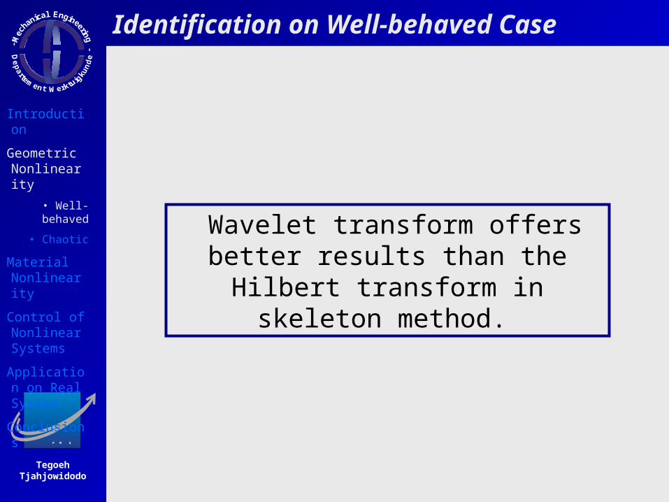
Identification on Well-behaved Case

Wavelet transform offers better results than the Hilbert transform in skeleton method.

Introduction


• Well-behaved

• Chaotic




Conclusions

Tegoeh Tjahjowidodo

P M A

W

Chaoticity in a system with backlash

m (kg)

k1 (N/m)

k0 (N/m)

c (Ns/m)

x0 (m)

CASE 1 1 0 40000 8 0.005 CASE 2 1 1000 31000 8 0.005

Schematic of mechanical system with backlash component

Example of parameters that lead to chaotic motion:

Introduction


• Well-behaved

• Chaotic




Conclusions

Tegoeh Tjahjowidodo

P M A

W

Chaotic response (1)

0 50 100 150 200-80

-60

-40

-20

0

20

40

Freq (Hz)

Pow

er S

pect

rum

(dB

)

0 0.5 1 1.5 2 2.5 3-20

-15

-10

-5

0

5

10

15

20

t (sec)

Dis

plac

emen

t (m

m)

CASE 1 was excited with sinusoidal signal with A=100 N and =40 rad/s

time (s) Freq. (Hz)

Dis

pla

cem

ent

(m

m)

Pow

er s

pect

rum

(dB

)

Introduction


• Well-behaved

• Chaotic




Conclusions

Tegoeh Tjahjowidodo

P M A

W

Chaotic response (2)

Phase plot and Poincaré map of case 1

displacement (mm)

velo

city

(m

m/s

)

Phase plot

displacement (mm)ve

loci

ty (

mm

/s)

Poincaré map

Introduction


• Well-behaved

• Chaotic




Conclusions

Tegoeh Tjahjowidodo

P M A

W

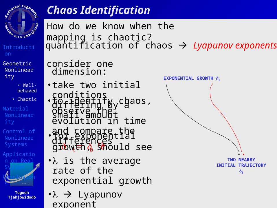
Chaos Identification

How do we know when the mapping is chaotic?

consider one dimension:• take two initial conditions

differing by a small amount

quantification of chaos Lyapunov exponents

• to identify chaos, observe the evolution in time and compare the differences

• for exponential growth, should see

• is the average rate of the exponential growth

• Lyapunov exponent

et 0t

Introduction


• Well-behaved

• Chaotic




Conclusions

EXPONENTIAL GROWTH t

▪ ▪TWO NEARBY

INITIAL TRAJECTORY 0

Tegoeh Tjahjowidodo

P M A

W

Dimensional Analysis

In order to examine the influence of each parameter on the nature of resulting response

02 /cos)p(p'"p F

mkc 02 0xkA 0

t0 0x/xp mk /02

0

primes indicate differentiation with respect to .

where:

1,1

1||,0

1,1

pp

p

pp

)p(F

tcosA)x(Fxcxm

Introduction


• Well-behaved

• Chaotic




Conclusions

Tegoeh Tjahjowidodo

P M A

W

Effect of Forcing Parameter and Backlash

0 1 2 3 4 5 6 7 8 9 100

0.05

0.1

0.15

0.2

0.25

k0x

0/A

Larg

est

Lyapunov E

xponent

2=0.042=0.02

1/

Larg

est

Lyap

unov

Exp

onen

t

1/=4.6

1/=3.4

Lyapunov exponent vs Forcing Parameter and/or Backlash SizeIntroduction


• Well-behaved

• Chaotic




Conclusions

Tegoeh Tjahjowidodo

P M A

W

Chaotic response in experimental setup

Phase plots of output responses for periodic signal with different excitation level

Introduction


• Well-behaved

• Chaotic




Conclusions

Tegoeh Tjahjowidodo

P M A

W

Noise Reduction in Chaotic Signal

Phase plots of output responses for periodic signal before and after noise reduction

• Simple Noise Reduction Methoddeveloped based on near future prediction

Introduction


• Well-behaved

• Chaotic




Conclusions

Tegoeh Tjahjowidodo

P M A

W

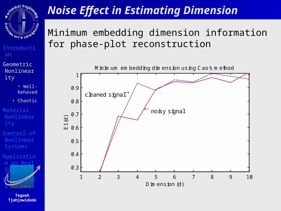
Noise Effect in Estimating Dimension

1 2 3 4 5 6 7 8 9 10

0.3

0.4

0.5

0.6

0.7

0.8

0.9

1

Dim ens ion (d)

E1

(d)Minim um em bedding dim ens ion us ing Cao's m ethod

cleaned signal

noisy signal

Minimum embedding dimension information for phase-plot reconstructionIntroduction


• Well-behaved

• Chaotic




Conclusions

Tegoeh Tjahjowidodo

P M A

W

Identification on Chaotic Case

Observing the chaos quantifier, e.g. Lyapunov exponent, could be used, in

principle, to estimate the parameter of a system.

Introduction


• Well-behaved

• Chaotic




Conclusions

Tegoeh Tjahjowidodo

P M A

W


Tegoeh Tjahjowidodo

P M A

W


Case study:mechanical system with friction element

Conventional friction model:

Coulomb modeldiscontinuity at zero velocity

velocity

frictionFriction is the result of a complex interaction

between two contact surfaces.

Introduction





Conclusions

Tegoeh Tjahjowidodo

P M A

W

Friction Characterisation

Two different friction regimes have been distinguished:

• the pre-sliding regime:appears predominantly as a function of displacement

• the sliding regime:function of sliding velocity

(Armstrong-Hélouvry, 1991,Canudas de Wit et al., 1995,

Swevers et al., 2000,Al-Bender et al., 2004)

f ,

Introduction





Conclusions

Tegoeh Tjahjowidodo

P M A

W

2

Pre-sliding regime (1)

0 (displacement)

Friction force

Pre-sliding friction

Friction force in pre-sliding regime not only depends on the output at some time instant in the past and the input, but also on past extremum values of the input or output as well.

hysteresis with non-local memory

11

2

y(q)

-y(-q)

y(q)

qm

Fm

-qm

2

3

x

x

4

Introduction





Conclusions

Tegoeh Tjahjowidodo

P M A

W

Pre-sliding regime (2)Equivalent dynamic parameters

The Describing Function technique is used to obtain the equivalent stiffness and damping:

y(q) is the virgin curve of the hysteresis

d)cos()cos(1yA

4k

02A

e

A

02e dq

2

)A(y)q(y

A

8c

displacement

fric

tion

Introduction





Conclusions

Tegoeh Tjahjowidodo

P M A

W

Pre-sliding friction model

ki

Wi

x

F

Alternative representation of hysteresis function with non-local memory for pre-sliding friction:

parallel connection of N elasto-slide elements

(Maxwell-Slip elements)

Introduction





Conclusions

Tegoeh Tjahjowidodo

P M A

W

Sliding regime

• When the motion is entering the sliding regime, in most cases, the Maxwell-Slip model is no longer suitable.

• The friction usually has a maximum value at the beginning and then continues to decrease with increasing velocity

Introduction





Conclusions

Tegoeh Tjahjowidodo

P M A

W

GMS friction model

Generalized Maxwell-Slip (GMS) model developed at PMA/KULeuven

vii k

dt

dF

– If the model is slipping:

)s(

FC)(

dt

dF

vvsgn i

ii

Mathematical representation of Maxwell-Slip elements

– If the model is sticking:

Introduction





Conclusions

Tegoeh Tjahjowidodo

P M A

W

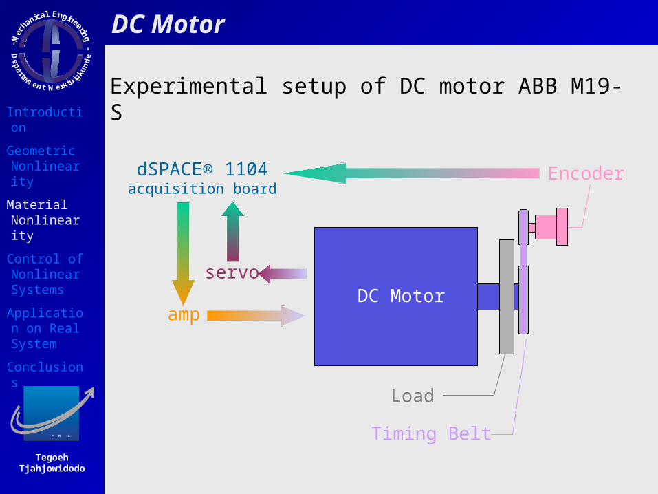
DC Motor

Experimental setup of DC motor ABB M19-S

Load

Timing Belt

Encoder

DC Motorservo

dSPACE® 1104acquisition board

amp

Introduction





Conclusions

Tegoeh Tjahjowidodo

P M A

W

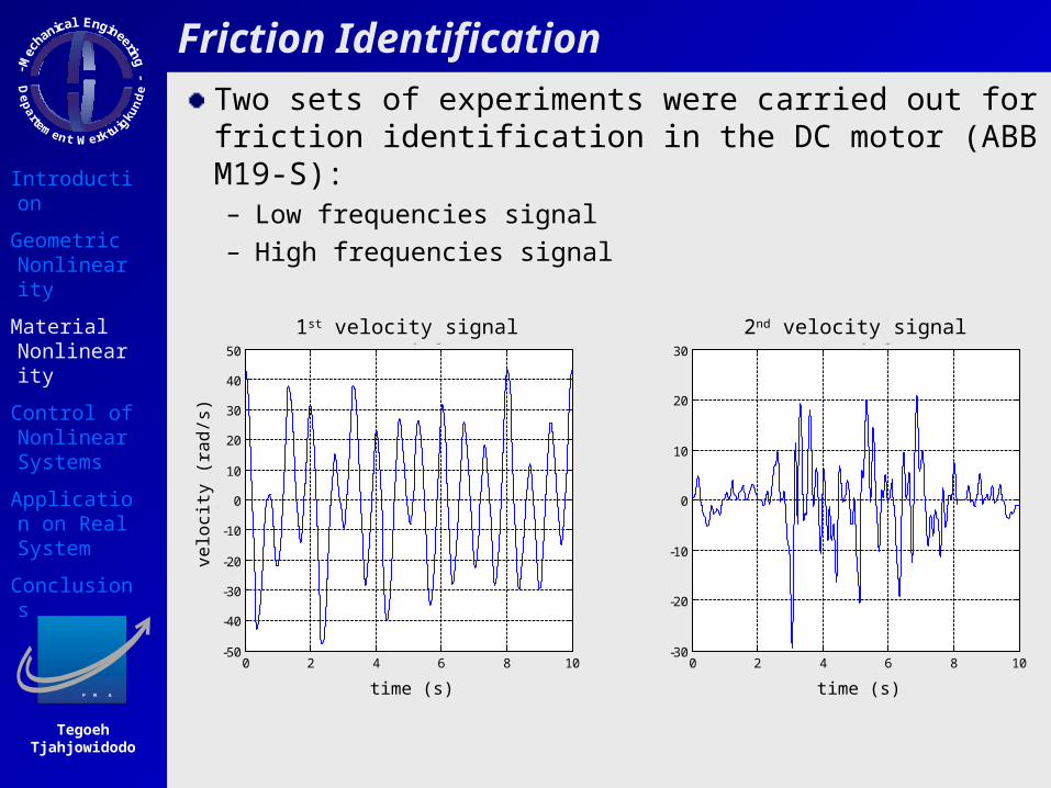
Friction Identification

Two sets of experiments were carried out for friction identification in the DC motor (ABB M19-S):– Low frequencies signal– High frequencies signal

0 2 4 6 8 10-50

-40

-30

-20

-10

0

10

20

30

40

50

time (s)

Ve

loc

ity

(ra

d/s

ec

)

1st velocity signal

0 2 4 6 8 10-30

-20

-10

0

10

20

30

time (s)

2nd velocity signal

Introduction





Conclusions

1st velocity signal 2nd velocity signal

time (s) time (s)

velo

city

(ra

d/s

)

Tegoeh Tjahjowidodo

P M A

W

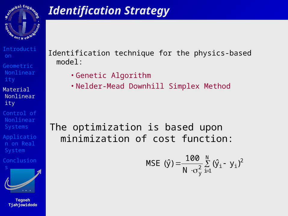
Identification Strategy

The optimization is based upon minimization of cost function:

N

iii

y

)yy(N

)y(MSE1

22

100

Identification technique for the physics-based model:

• Genetic Algorithm• Nelder-Mead Downhill Simplex Method

Introduction





Conclusions

Tegoeh Tjahjowidodo

P M A

W

Identification Results #1Identification results of low frequencies experiment:

1 2 3 4 5 6

-10

-5

0

5

10

Coulomb model

time (s)

To

rqu

e (

Nm

)

eps=0.1

1 2 3 4 5 6

-10

-5

0

5

10

Exponential Coulomb model

time (s)

eps=0.1

Coulomb model

torq

ue

(N

m)

1 2 3 4 5 6

-10

-5

0

5

10

LuGre model

time (s)

To

rqu

e (

Nm

)

1 2 3 4 5 6

-10

-5

0

5

10

GMS model

time (s)

GMS model

time (s)

Introduction





ConclusionsLuGre model

time (s)

torq

ue

(N

m)

1 2 3 4 5 6

-10

-5

0

5

10

LuGre model

time (s)

To

rqu

e (

Nm

)

1 2 3 4 5 6

-10

-5

0

5

10

GMS model

time (s)


1 2 3 4 5 6

-10

-5

0

5

10

Coulomb model

time (s)

To

rqu

e (

Nm

)

eps=0.1

1 2 3 4 5 6

-10

-5

0

5

10


time (s)

eps=0.1Coulomb 2.06% (0.3770)

Exp-Coulomb 2.06% (0.3360)

LuGre 2.03% (0.3530)

GMS 1.97% (0.3470)

MSE (max.err.)

Tegoeh Tjahjowidodo

P M A

W

Identification Results #2Identification results of high frequencies experiment:

time (s)

0 2 4 6 8 10-15

-10

-5

0

5

10

15

time (s)

Err

or

Coulomb Model

0 2 4 6 8 10-15

-10

-5

0

5

10

15

time (s)

Exponential-Coulomb ModelCoulomb model

torq

ue

(N

m)

Introduction





Conclusions

0 2 4 6 8 10-15

-10

-5

0

5

10

15

time (s)

To

rqu

e (

Nm

)

LuGre Model

0 2 4 6 8 10-15

-10

-5

0

5

10

15

time (s)

GMS ModelLuGre model

torq

ue

(N

m)


0 2 4 6 8 10-15

-10

-5

0

5

10

15

time (s)

Err

or

Coulomb Model

0 2 4 6 8 10-15

-10

-5

0

5

10

15

time (s)

Exponential-Coulomb Model

GMS model

time (s)

0 2 4 6 8 10-15

-10

-5

0

5

10

15

time (s)

To

rqu

e (

Nm

)

LuGre Model

0 2 4 6 8 10-15

-10

-5

0

5

10

15

time (s)

GMS Model

MSE (max.err.)

Coulomb 17.92% (1.2993)

Exp-Coulomb 9.59% (1.2604)

LuGre 4.30% (0.6466)

GMS4 1.39% (0.5711)

GMS10 1.19% (0.5177)

Tegoeh Tjahjowidodo

P M A

W

Identification on Material Nonlinearity Case

Friction identification is possible to be conducted using a single experiment. However, selection of the excitation signal plays an important role for

the identification step.

Introduction





Conclusions

Tegoeh Tjahjowidodo

P M A

W


Tegoeh Tjahjowidodo

P M A

W

Overview of Controllers

Model-based controllers

– Linear Controllers• PD controller

• Cascade controller (combine position-speed loops)

– Nonlinear Controllers• Discontinuous Nonlinear Proportional Feedback (DNPF)

controller

• Gain Scheduling controller

Introduction





Conclusions

Qh

-Qh

Position error (e)

Controlinput (u)

adds an extra compensating torque when the position error is within pre-sliding region

developed based on the equivalent dynamic parameters of the system.

Tegoeh Tjahjowidodo

P M A

W

Gain Scheduling Controller (1)

treats two different regimes of friction in separated modes.

The first mode

The corresponding gains are designed and optimized at some points (of amplitude of motion) regarding a certain

performance criteria.

• when the system is moving in the sliding region• linear controller + equivalent Coulomb friction model

• when the system is moving in the pre-sliding region• adjusts proportional (kp) and derivative (kd) gain based on

the equivalent dynamic parameter

The second mode

Introduction





Conclusions

Tegoeh Tjahjowidodo

P M A

W

Gain Scheduling Controller (2)

Look-up table of the gains

System SWITCHING FUNCTION

x

du dt |.|=0

memorize =x |x- |<Q

h

and |x- |

-

+

xd

PD

F du dt

- +

+ -

PD

1st m

od

e2n

d m

od

e

Gain Scheduling StrategyIntroduction





Conclusions

Tegoeh Tjahjowidodo

P M A

W

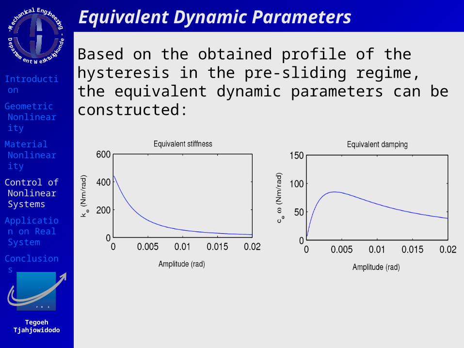
Equivalent Dynamic Parameters

Based on the obtained profile of the hysteresis in the pre-sliding regime, the equivalent dynamic parameters can be constructed:

Introduction





Conclusions

Tegoeh Tjahjowidodo

P M A

W

Gain Scheduling Design

• By using the obtained equivalent dynamic parameters, some PD gains at different selected amplitudes are optimized.

• The optimal gains are interpolated for intermediate points.

Introduction





Conclusions

Tegoeh Tjahjowidodo

P M A

W

Control Objectives

In the point-to-point (PTP) positioning system, a high accuracy and a short transition time are the most important performance criteria, while the path of the motion is less significant.

High accuracy and fast response speed with no overshoots are desired.

Performance criteria:Introduction





Conclusions

Tegoeh Tjahjowidodo

P M A

W

Step Input

-

The step responses to a 0.4 rad step input are appraised.

Introduction





Conclusions

Tegoeh Tjahjowidodo

P M A

W

Step Response ResultStep responses of the system using the proposed gain scheduling controller in comparison with the PD, cascade and DNPF controllers.Introduction





Conclusions

Tegoeh Tjahjowidodo

P M A

W

Control of Nonlinear System

Model based control is able to yield good results, depending on the models used and the control

strategy.

Introduction





Conclusions

Tegoeh Tjahjowidodo

P M A

W

Application on a Real System

(Harmonic Drive)

Tegoeh Tjahjowidodo

P M A

W

The Harmonic Drive

Invented by C. Walton Musser in 1955.

Originally labeled ‘strain-wave gearing’, which employs a continuous deflection wave along a non-rigid gear to allow gradual engagement of gear teeth.

Can provide very high reduction ratios in a very small package.

Introduction





• Identification

• Control

Conclusions

Tegoeh Tjahjowidodo

P M A

W

The Harmonic Drive components

WAVE DRIVE®

(has 2 more teeth than flexspline)

Introduction





• Identification

• Control

Conclusions

Tegoeh Tjahjowidodo

P M A

W

Operating mechanism

Operating principle of harmonic drive

Introduction





• Identification

• Control

Conclusions

Tegoeh Tjahjowidodo

P M A

W

Scope of Harmonic Drive Research

Torsional Stiffness:– apparently due to deformation of the wave generator, and an increase in

gear-tooth contact area with increasing load (Nye, 1991).– displays a ‘soft wind-up’ behavior, which is characterized by very low

stiffness at low applied load (Kircanski, 1997).

Frictional Losses:– occurs primarily at the gear-tooth interface– Friction in Harmonic Drive is strongly position dependent due to kinematic

error (Kennedy, 2003).

Kinematic error:– caused by a number of factors, such as tooth-placement errors, out-of-

roundness in HD components, and misalignment during assembly.– The error signature can display frequency components at two cycles per

wave-generator revolution (Tuttle, 1992).

Introduction





• Identification

• Control

Conclusions

Tegoeh Tjahjowidodo

P M A

W

Torsional Stiffness - definition

Torsional stiffness is measured by locking the wave generator to the circular spline and applying loads

to a link subjected to the flexspline.

Introduction





• Identification

• Control

Conclusions

Tegoeh Tjahjowidodo

P M A

W

Torsional Stiffness – experiments (1)

load cell

Bentley probe

Lock thewave-generator

Experiment was carried out on WAVE DRIVE® component:

Introduction





• Identification

• Control

Conclusions

Tegoeh Tjahjowidodo

P M A

W


Stiffness curve obtained from sine excitation:Introduction





• Identification

• Control

Conclusions

-0.05 -0.04 -0.03 -0.02 -0.01 0 0.01 0.02 0.03 0.04-0.2

-0.15

-0.1

-0.05

0

0.05

0.1

0.15

0.2

Torque

To

rsio

nT

orsi

on (

rad)

Torque (Nm)

-0.4 -0.3 -0.2 -0.1 0 0.1 0.2 0.3 0.4

3

0

2

1

-1

-2

-3

-4

4

×10-3

Tegoeh Tjahjowidodo

P M A

W


Stiffness curve obtained from triangular-wave excitation(with varying amplitudes):

Introduction





• Identification

• Control

Conclusions

-0.04 -0.03 -0.02 -0.01 0 0.01 0.02 0.03 0.04

-0.1

-0.05

0

0.05

0.1

0.15

Torque

To

rsio

n

Tor

sion

(ra

d)

Torque (Nm)

3.75

0

2.50

1.25

-1.25

-2.50

-0.4 -0.3 -0.2 -0.1 0 0.1 0.2 0.3 0.4

time (s)

3.75

0

2.50

1.25

-1.25

-2.50

0 2 4 6 8

×10-3

Tegoeh Tjahjowidodo

P M A

W

Piecewise linear model

Hysteresis models

Torsional Stiffness Models

x

F

k1

x0

-x0

x

F

k0

Two different approach of models:Introduction





• Identification

• Control

Conclusions

Tegoeh Tjahjowidodo

P M A

W

Schematic of torsional stiffness model

Proposed model of torsional stiffness:Maxwell-slip elements

+hardening spring

elementarystick-slip 1

x

T

Pre-sliding friction

hardening spring

elementarystick-slip N

Introduction





• Identification

• Control

Conclusions

Tegoeh Tjahjowidodo

P M A

W

Torsional Stiffness – hysteresis model (1)

Identification results:

Introduction





• Identification

• Control

Conclusions

-0.03 -0.02 -0.01 0 0.01 0.02 0.03

-0.1

-0.05

0

0.05

0.1

0.15

Torque

To

rsio

n

Torsional Stiffness of Flexspline Component

Tor

sion

(ra

d)

Torque (Nm)

Torsional Stiffness

-0.3 -0.2 -0.1 0 0.1 0.2 0.3

3

0

2

1

-1

-2

×10-3

Tegoeh Tjahjowidodo

P M A

W

Torsional Stiffness – hysteretic model (2)

Identification results:

1.14% MSE

(MSE of piecewise linear model: 8.7%)

Introduction





• Identification

• Control

Conclusions

0 5 10 15 20 25 30-0.04

-0.02

0

0.02

0.04

To

rqu

e

ActualModel

0 5 10 15 20 25 30-0.04

-0.02

0

0.02

0.04

Err

or

Time (s)

Err

or (

Nm

)T

orqu

e (N

m)

Time (sec)

0.4

0.2

0

-0.2

-0.4

0.4

0.2

0

-0.2

-0.40 5 10 15 20 25 30

0 5 10 15 20 25 30

Tegoeh Tjahjowidodo

P M A

W

Control of Mechanical System with HD

System apparatus:

Introduction





• Identification

• Control

Conclusions

FHA-C mini servo actuator gear set with AC servo motor in one compact package

Tegoeh Tjahjowidodo

P M A

W

FHA-C mini servo actuator

Schematic drawing of FHA-C

TkS kH

TF

m1 m2m3

armature inertia circular-spline inertiaload inertia

friction in the motor torsional stiffness of the HDcomplete-close package

Friction in the DC motor and torsional stiffness in the gear set cannot be

identified separately.

Introduction





• Identification

• Control

Conclusions

Tegoeh Tjahjowidodo

P M A

W

Control of FHA-C mini servo actuator

Two different approaches are considered for control purposes:

First approach: a mass on a frictional surface

meqT

Tf

Second approach: two masses connected by a hysteresis torsional spring

m3keqm1T

Introduction





• Identification

• Control

Conclusions

Tegoeh Tjahjowidodo

P M A

W

2nd Approach - Two masses and hysteresis spring (1)

Assumption:Neglect the external hysteretic nonlinearity source.

Nonlinearity mainly comes from the torsional stiffness

The torsional stiffness is identified by locking the output shaft and measuring the motor current.

Introduction





• Identification

• Control

Conclusions

Tegoeh Tjahjowidodo

P M A

W

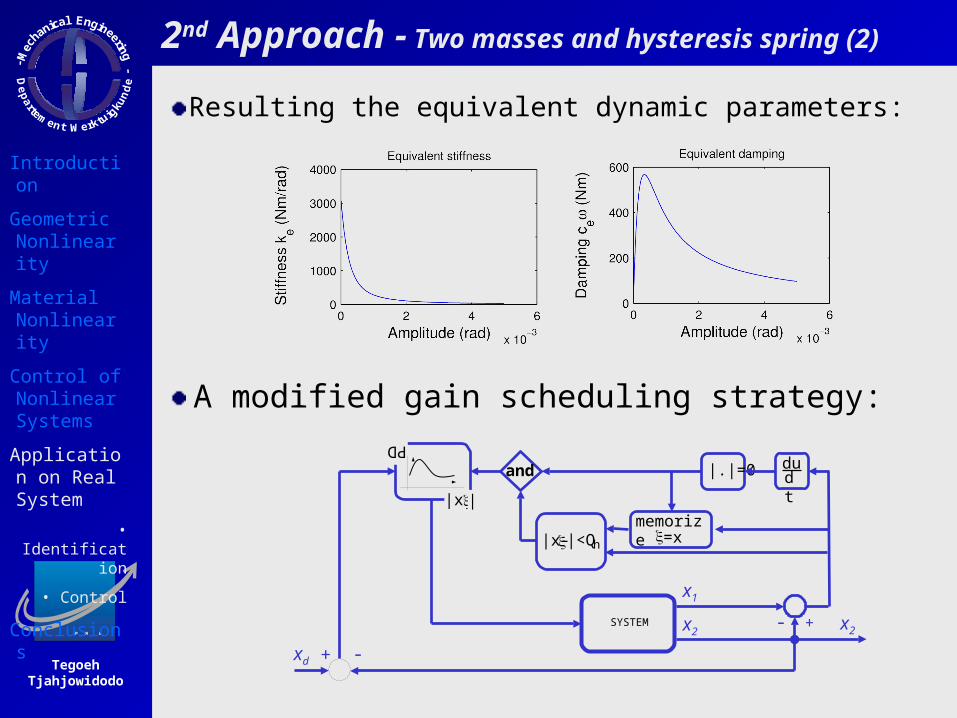
2nd Approach - Two masses and hysteresis spring (2)

Resulting the equivalent dynamic parameters:

A modified gain scheduling strategy:

xd

SYSTEM

memorize =x|x-|<Qh

dudt

|.|=0and

PD

|x-|

+ -

x2

x1

- + x2

Introduction





• Identification

• Control

Conclusions

Tegoeh Tjahjowidodo

P M A

W

Control Results of 2nd Approach (1)

Step response to a 0.2 rad step input

Introduction





• Identification

• Control

Conclusions

Tegoeh Tjahjowidodo

P M A

W

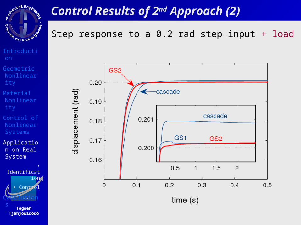
Control Results of 2nd Approach (2)

Step response to a 0.2 rad step input + load

Introduction





• Identification

• Control

Conclusions

Tegoeh Tjahjowidodo

P M A

W

Application on a System with HD

A piecewise linear model together with non-local memory hysteresis resolve the difficulties in

determining the model of torsional stiffness in harmonic drive.

Introduction





• Identification

• Control

Conclusions

Tegoeh Tjahjowidodo

P M A

W

Conclusions

Two cases for a nonlinear system with ‘well-behaved’ and chaotic response for a periodic input have been addressed and appropriate identification methods are developed for each.

Identification of systems with material nonlinearity (friction) utilizing single experiment is feasible to be carried out.

Detailed understanding of a physical system is playing an important role in achieving a controller with high performance.

Identification of a system, in which the two nonlinearity sources are manifested, has been conducted successfully.

Introduction





Conclusions

Tegoeh Tjahjowidodo

P M A

W

Future work

Combining the advantages of Hilbert and wavelet transform in order to improve the skeleton techniques.

Implementation of the skeleton technique for a real higher-degree-of-freedom system.

Further study for the applicability of the GMS model to any friction conditions.

Extension of the identification and control methods to higher-degree-of-freedom systems with two (or more) hysteresis (material) nonlinearities.

Introduction





Conclusions

Tegoeh Tjahjowidodo

P M A

W

Introduction





Conclusions

Documents

Tegoeh Tjahjowidodo Characterization, Modelling and Control of Mechanical Systems Comprising Material and Geometrical Nonlinearities Tegoeh Tjahjowidodo