Embed Size (px)
Citation preview

Working Paper/Document de travail
2007-7
Technology Shocks and Business Cycles:
The Role of Processing Stages and
Nominal Rigidities
by Louis Phaneuf and Nooman Rebei
www.bankofcanada.ca

Bank of Canada Working Paper 2007-7
February 2007
Technology Shocks and Business Cycles:The Role of Processing Stages and
Nominal Rigidities
by
Louis Phaneuf1 and Nooman Rebei2
1Department of EconomicsUniversité du Québec à Montréal
Montréal, Quebec, Canada H3C 3P8and CIRPÉE
2Research DepartmentBank of Canada
Ottawa, Ontario, Canada K1A [email protected]
Bank of Canada working papers are theoretical or empirical works-in-progress on subjects ineconomics and finance. The views expressed in this paper are those of the authors.
No responsibility for them should be attributed to the Bank of Canada.
ISSN 1701-9397 © 2007 Bank of Canada

ii
Acknowledgements
The authors are grateful to Martin Eichenbaum, Jonas Fisher, Jordi Galí, Peter Ireland,
Maher Khaznaji, Zheng Liu, Ellen McGrattan, Rhys Mendes, Nicolas Petrosky-Nadeau and
seminar participants at the Bank of Spain for useful comments. Phaneuf acknowledges financial
support from FQRSC and SSHRC.

iii
Abstract
This paper develops and estimates a dynamic general equilibrium model that realistically
accounts for an input-output linkage between firms operating at different stages of processing.
Firms face technological change which is specific to their processing stage and charge new prices
according to stage-specific Calvo-probabilities. Only a fixed fraction of households have an
opportunity to adjust nominal wages to new information each period. Intermediate-stage
technology shocks account for the bulk of output variability at business cycle frequencies, while
final-stage technology shocks do not explain much. Although technology shocks drive the
business cycle, the model predicts weakly procyclical real wages, and a near-zero correlation
between return to working and hours worked. Furthermore, the model has rich implications for
the dynamics of business cycles.
JEL classification: E32Bank classification: Business fluctuations and cycles; Economic models
Résumé
Les auteurs élaborent et estiment un modèle dynamique d’équilibre général où est représentée
avec réalisme la relation qui lie, par le biais des intrants et des extrants, les entreprises intervenant
aux diverses étapes du processus de production. Les chocs technologiques subis diffèrent selon
que l’entreprise se charge de l’étape intermédiaire ou de l’étape finale de la production, tout
comme la probabilité qu’elle révise ses prix à chaque période (dans un cadre à la Calvo). À
chaque période également, une proportion fixe des ménages voient leur salaire nominal modifié à
la lumière des nouvelles données reçues. Les chocs qui touchent les techniques de fabrication à
l’étape intermédiaire expliquent le gros de la variabilité de la production au cours du cycle
économique, alors que ceux qui concernent l’étape de production finale en expliquent fort peu.
Même si les chocs technologiques sont à l’origine de la plupart des fluctuations du cycle
économique dans le modèle, l’évolution du salaire réel se révèle faiblement procyclique, et la
corrélation entre la productivité et le nombre d’heures travaillées s’avère presque nulle. Enfin, le
modèle parvient fort bien à décrire la dynamique des cycles économiques.
Classification JEL : E32Classification de la Banque : Cycles et fluctuations économiques; Modèles économiques

1 Introduction
This paper develops a dynamic general equilibrium (DGE) framework that sheds new light on the
cyclical effects of technological change while offering new evidence of the importance of technology
shocks for business cycles. Most macroeconomic models, from standard real business cycle (RBC)
models to DGE models featuring nominal rigidities and/or real frictions, assume that firms operate
at the final stage of production, hence facing technological change only at this single processing
stage. However, in reality the production of several finished goods typically goes through more
than one stage of processing. This simple fact forces some potentially important questions about
the role of technological change as a source of business cycles. Can technology shocks at other than
the final stage have an impact on aggregate fluctuations? If so, is this effect large quantitatively? If
technology shocks are found to contribute substantially to business cycles in a model with multiple
processing stages, does the same model help remedy the anomalies that have plagued a large class
of DGE models in which technological change is the dominant source of aggregate fluctuations?
Our paper provides affirmative answers to these questions using an estimated DGE model with
five main features. First, our model embeds a two-stage production and pricing structure. The
production of finished goods goes through two stages of processing: a stage of intermediate goods
and a stage of finished goods. Unlike most existing models, our framework assumes that firms
face productivity shocks which are specific to their stage of processing. Firms at the intermediate
stage use capital and labor to produce intermediate goods, while firms at the final stage utilize
a composite of goods fabricated at the intermediate stage as intermediate inputs, in addition to
capital and labor, to produce finished goods. Recent contributions by Basu (1995) and Huang,
Liu and Phaneuf (2004) suggest that combining nominal rigidities with an input-output structure
helps understand some important aspects of reality. However, instead of assuming that firms are
linked through a horizontal roundabout input-output structure within a single stage of production
as these authors do, we focus on an input-output linkage between firms operating at different stages
of processing. Our framework is thus closer in spirit to the model of Huang and Liu (2005) that
incorporates an input-output linkage between sectors to analyze the design of optimal monetary
policy with several sources of nominal price rigidities.1
Second, nominal prices at both stages of processing are determined by staggered Calvo-contracts,
producers at each stage responding to a stage-specific probability of reoptimizing their prices in
each period. Hence, unlike the class of models featuring sticky prices only at the final stage of pro-1Also, Huang and Liu (2001) propose a DGE model of the transmission of monetary shocks that stresses production
chains and Taylor’s (1980) staggered price contracts.
2

cessing, our model accounts for nominal price rigidities at different stages of production. Therefore,
a key characteristic of our framework compared to standard sticky-price models is that changes in
the relative price of intermediate goods to final goods can have an allocative role.
Third, households are imperfectly competitive with respect to labor skills. The nominal wages
of different skills are also determined by Calvo-contracts.2 The preferences of households are
subject to a shock. Preference shocks have sometimes been identified as the main source of cyclical
movements in output and hours worked during the postwar period [e.g., Shapiro and Watson (1988),
Hall (1997) and Galı and Rabanal (2004)].3
Fourth, our model includes real rigidities in the form of costs of adjusting the stock of physical
capital and hours worked. Kim (2000) provides evidence showing that capital adjustment costs had
a significant impact on business cycle fluctuations, while Ambler, Guay and Phaneuf (2006) show
that labor adjustment costs and sticky nominal wages have been first-order elements in shaping
U.S. postwar business cycle dynamics.
The fifth ingredient in our model is a monetary policy rule that sets short-term interest rates
in response to variations in finished-good inflation and final output measured in deviations from
their steady-state values. Following Rotemberg and Woodford (1999) and Clarida, Galı and Gertler
(2000), our specification allows for interest-rate smoothing, and therefore includes the lagged in-
terest rate. However, some authors have questioned whether the lagged rate is a fundamental
component of the policy rule. They argue that the apparent significance of the lagged rate in
estimated rules could be attributed to serially correlated errors or Fed’s response to factors not
included in the policy rule [e.g., Rudebusch (2002) and English, Nelson and Sack (2003)]. Hence,
the policy rule incorporates both the lagged interest rate and serially correlated policy errors.
We estimate the structural parameters of our models and various second moments of the data
using postwar U.S. quarterly data and a maximum likelihood procedure similar to the one imple-
mented in Ireland (2003, 2004a, 2004b). Our main findings can be summarized as follows. First,
according to our estimates, the two-stage production and pricing structure is strongly supported
by the data. The key structural parameters of the model, including the share of intermediate goods
entering the fabrication of finished goods and the parameters governing nominal contracts and real
frictions, are economically meaningful and statistically significant. The price contracts of finished2Thus, our model features both nominal wage and price rigidities. Other examples of DGE models with both
types of nominal rigidity include Huang, Liu and Phaneuf (2004) and Christiano, Eichenbaum and Evans (2005),
among others. However, these models have only one stage of production.3Ireland (2004a) also finds that preference shocks had a strong impact on the variability of inflation during the
postwar period.
3

goods are shorter than the price contracts of intermediate goods, the former lasting on average 2.9
quarters compared to 3.3 quarters for the later. Wage contracts last longer on average than price
contracts. Also, we find no evidence of interest-rate smoothing or highly serially correlated policy
shocks.
Second, intermediate-stage technology shocks account for the bulk of output variability at busi-
ness cycle frequencies (contributing for example to 31, 52 and 62% of the one, four and eight-quarters
ahead forecast errors of final output). The strong impact of intermediate-stage productivity shocks
on final output can be explained as follows. An intermediate-stage technology improvement is
followed, by a persistent, hump-shaped decline in the relative price of intermediate goods to final
goods and by a persistent, hump-shaped increase in the production of intermediate goods. With
intermediate-stage output strongly increasing, finished-good firms use more intermediate inputs,
and thus final output rises. Also, following a positive shock to intermediate-stage technology, real
wages initially decline. The fall in real wages further boosts hours worked and final output.
Third, intermediate-stage technology shocks generate rich business-cycle dynamics, produc-
ing persistent, hump-shaped responses of final output, consumption, investment and total hours
worked. Hence, the model meets the challenge posed by King, Plosser and Rebelo (1988) who have
shown that the standard neoclassical growth model does not account for the dynamics of output,
investment and hours as it fails to produce hump-shaped impulse responses following technology
shocks.4
Meanwhile, final-stage technology shocks explain only a small percentage of the cyclical variance
of final output (less than 10% at business cycle frequencies). A positive shock to final-stage tech-
nology is followed by a relatively small increase in the relative price of intermediate goods to final
goods. Furthermore, it is followed by a persistent, hump-shaped increase in real wages. Therefore,
intermediate-stage hours and output decline. Final-stage hours also fall, and with finished-good
firms using less intermediate inputs, the increase in final output is relatively small and lasts only for
a few periods. Thus, a unique feature of the estimated two-stage model lies in its ability to predict
that total hours worked may either rise or fall following a technology improvement depending on
the source of technological change.
Fourth, we find that monetary policy shocks have a significant impact on economic fluctuations
at very short horizons, but that their real effects rapidly decline at longer horizons. This finding
is broadly consistent with the evidence across different branches of the literature using VARs or4Focusing on the dynamics of output, Cogley and Nason (1995) reach a a similar conclusion for a wide range of
RBC models.
4

estimated DGE models. However, in contrast to the empirical findings of previous estimated DGE
models, monetary policy shocks explain a high percentage (more than 70%) of the variability of
finished-good inflation at all horizons. Still, technology shocks account for a non negligible fraction
of the variability of finished-good inflation (about one fourth). Furthermore, unlike what other
researchers have found using single-stage models, preference shocks have a very small impact on
fluctuations of hours and output, and almost no effect on the variability of inflation.
Next, the paper turns its attention to the model’s ability to account for a fairly comprehensive
set of business-cycle statistics. We first look at the size of fluctuations implied by the two-stage
model. It accounts very well for the volatility of hours worked relative to volatility of output in
the postwar period. Also, the model correctly predicts that output is about twice as volatile as
return to working. Several business cycle models have not been able to simultaneously explain these
two facts [see Hansen (1985) and Hansen and Wright (1992)]. Furthermore, if the price index of
finished goods is approximated by the consumer price index (or GDP deflator) while the price index
of intermediate goods roughly corresponds to the producer price index, the model predicts that rate
of inflation of finished goods is only about half as volatile as the rate of inflation of intermediate
goods, just as in the data.
Extending our analysis to some key comovements, we show that the correlation between total
hours and final output is both positive and high. The intermediate-stage technology shock is the
key source giving rise to this comovement. The two-stage model also accounts for the so-called
Dunlop-Tarshis observation or absence of a strong countercyclical pattern in real wages. Recently,
Christiano and Eichenbaum (1992) have reinterpreted the Dunlop-Tarhsis observation in the context
of modern business cycle analysis as the near-zero correlation between hours worked and return
to working. Our model predicts that real wages are weakly procyclical and that the correlation
between hours and productivity is close to zero, as we find in the data. Most business cycle models
where technology shocks are a driving force counterfactually predict that real wages are highly
procyclical and that the correlation between hours and productivity is both positive and high.
The model’s success in explaining these two critical comovements mostly reflects the fact that
hours respond very differently to technology shocks depending on the specific source of technological
change. Taking, for example, the correlation between return to working and hours, a positive
shock to final-stage technology induces a negative comovement between these variables, while the
intermediate-stage technology shock generates a positive correlation. Thus, the correlation between
hours and productivity produced by the two technology shocks is close to zero, which stands in
stark contrast with the predictions of typical RBC models.
5

Finally, to better understand our model’s driving mechanism, we estimate two models that are
special cases of our general framework. The first model variant assumes that all firms operate
at the final stage, and thus features only one technology shock and a single source of nominal
price rigidity. This variant resembles new keynesian models. The second model incorporates the
two-stage processing structure, while assuming that wages and prices are perfectly flexible. This
variant is closer in spirit to RBC models. As the general framework nests the two model variants,
a formal likelihood ratio test can be performed to determine which model is preferred by the data.
The general framework is easily preferred to the model variants.
The paper is organized as follows. Section 2 provides a description of our two-stage production
and pricing model. Section 3 discusses some econometric issues, data and calibration. Section 4
presents and analyzes our main findings. Section 5 offers concluding remarks.
2 The Model
The economy is inhabited by a large number of infinitely lived households endowed with differenti-
ated labor skills. Households have preferences defined over expected streams of consumption goods,
real balances and leisure. In each period, they face a constant probability of adjusting nominal
wages. Firms at the intermediate and final stages produce differentiated goods. Finished-good
firms utilize a composite of intermediate-stage products as intermediate inputs. Firms experience
exogenous technological change which is specific to their processing stage. Producers in each period
adjust nominal prices in response to a stage-specific Calvo-probability. The stock of physical capital
and hours worked are both costly to adjust.
2.1 The Households
We assume a continuum of households indexed by i, with i ∈ (0, 1) denoting a particular type of
labor skill. Household i′s preferences are described by the following expected utility function:
U(i)0 = E0
∞∑
t=0
βt
[γ
γ − 1κt log
(Ct(i)
γ−1γ + b
1γ
(Mt(i)Py,t
) γ−1γ
)− µ
Nt(i)1+η
1 + η
], (1)
where β is a discount factor, Ct(i) is real consumption, Mt(i)/Py,t stands for real money balances,
Mt(i) is the nominal money stock, Py,t is the price index of finished goods, and Nt(i) represents
hours worked; γ, b, µ and η are positive structural parameters, and γ and η represent the constant
elasticity of substitution between consumption and real balances, and the inverse of the elasticity
6

of labor supply, respectively. The representative household’s total time available is normalized to
one in each period.
The preference shock, κt, has the time-series representation:
log(κt) = ρκ log(κt−1) + εκ,t, (2)
where εκ,t is a serially uncorrelated independent and identically distributed process with a mean-
zero and a standard error σκ.
The household i′s budget constraint is
Ct(i) + It(i) + CACt(i) +Mt(i)Py,t
+Bt+1(i)
Py,t
=Wt(i)Py,t
Nt(i) +Qt
Py,tKt(i) +
Mt−1(i)Py,t
+ Rt−1Bt(i)Py,t
+Dy,t(i)Py,t
+Dz,t(i)Py,t
+Tt(i)Py,t
, (3)
where It(i) is real investment, CACt(i) is the real cost of adjusting the stock of physical capital
Kt(i), Bt+1(i) represents bonds carried in period t+1, Wt(i) is the nominal wage, Qt is the nominal
rental rate of capital, Rt−1 is the gross nominal interest rate between period t − 1 and period t,
Dy,t(i) and Dz,t(i) are the nominal dividends paid to the household by the finished-good firms and
by the intermediate-good firms, respectively, and Tt(i) is a lump-sum nominal transfer from the
monetary authority.
The cost-function for the adjusting the stock of physical capital is
CACt(i) =ϕk
2
(Kt+1(i)Kt(i)
− 1)2
Kt(i), (4)
where ϕk > 0 is the cost parameter.
The investment technology is
It(i) = Kt+1(i)− (1− δ)Kt(i), (5)
where δ ∈ (0, 1) is the rate of depreciation of physical capital.
Aggregate labor input, Nt, is a composite of all labor skills,
Nt =(∫ 1
0Nt(i)
σ−1σ di
) σσ−1
, (6)
where σ represents the elasticity of substitution between skills. Labor demand for skill i is,
7

Nt(i) =(
Wt(i)Wt
)−σ
Nt, (7)
where Wt is the wage rate of the composite skill, given by
Wt =(∫ 1
0Wt(i)1−σdi
) 11−σ
. (8)
Household i chooses Ct(i), Mt(i), Bt+1(i), Kt+1(i) and Wt(i) (whenever nominal wages can
be adjusted), that maximize the expected discounted sum of utility flows, subject to the budget
constraint and the firms’ labor demand for skill i. The first-order conditions for this problem are:
κtCt(i)−1γ
Ct(i)γ−1
γ + b1γ
t
(Mt(i)Py,t
) γ−1γ
= λt(i), (9)
κtb1γ
t
(Mt(i)Py,t
)−1γ
Ct(i)γ−1
γ + b1γ
t
(Mt(i)Py,t
) γ−1γ
= λt(i)(
1− 1Rt
), (10)
βEtλt+1(i)λt(i)
[qt+1 + 1− δ + ϕk
(Kt+2(i)Kt+1(i)
− 1)
Kt+2(i)Kt+1(i)
− ϕk
2
(Kt+2(i)Kt+1(i)
− 1)2
]
= 1 + ϕkEt
(Kt+1(i)Kt(i)
− 1)
, (11)
and
λt(i) = βRtEt
(λt+1(i)πy,t+1
), (12)
where λt(i) is the nonnegative Lagrange multiplier associated with the budget constraint, qt =
Qt/Py,t, and πy,t+1 is the rate of inflation of finished goods.
2.1.1 The Wage Decision
In each period, nominal wages are adjusted with probability 1− dw. The first-order condition with
respect to Wt(i) is
Wt(i) =σ
σ − 1Et
∑∞q=0(βdw)qNt+q(i)η+1
Et∑∞
q=0(βdw)qNt+q(i)λt+q(i) 1Py,t+q
. (13)
8

At the symmetric equilibrium, the aggregate nominal wage is given by the following recursive
equation:
Wt =[dwW 1−σ
t−1 + (1− dw)W 1−σt
] 11−σ
, (14)
where Wt is the optimal or average nominal wage of workers who can revise their wages in period
t.
2.2 Firms and Processing Stages
Firms producing at different stages are related by an input-output linkage. Producers also charge
different prices at each stage. In each period, the nominal prices of finished goods have a probability
dy of staying constant, while the probability that the prices of intermediate goods stay put is dz.
2.2.1 Final Stage
Final output, Yt, is a composite of all finished goods Yt(j), j ∈ (0, 1) denoting a particular type of
finished good,
Yt =(∫ 1
0Yt(j)
θy−1
θy dj
) θyθy−1
,
where θy is the elasticity of substitution between finished goods.
Finished-good firm j maximizes profits, solving the following problem
maxYt(j)
Py,t
(∫ 1
0Yt(j)
θy−1
θy dj
) θyθy−1 −
∫ 1
0Py,t(j)Yt(j)dj.
where Py,t(j) is the nominal price of finished good j. Profit maximization yields the following
first-order condition for the demand of finished good j,
Yt(j) =(
Py,t(j)Py,t
)−θy
Yt. (15)
The price index Py,t is given by
Py,t =(∫ 1
0Py,t(j)1−θydj
) 11−θy
.
9

2.2.2 Intermediate Stage
Output at the intermediate stage of processing, Zt, is a composite of all intermediate goods Zt(l),
l ∈ (0, 1) denoting a type of intermediate good,
Zt =(∫ 1
0Zt(l)
θz−1θz dl
) θzθz−1
,
where θz is the elasticity of substitution between intermediate goods.
Profit maximization yields the following first-order condition for the demand of intermediate
good l,
Zt(l) =(
Pz,t(l)Pz,t
)−θz
Zt, (16)
where Pz,t(l) is the price of intermediate good l, and Pz,t represents the price index of intermediate
goods. Price index Pz,t is given by
Pz,t =(∫ 1
0Pz,t(l)1−θzdl
) 11−θz
.
2.2.3 Finished–Good Firms
The production of finished good j requires the use of labor Ny,t(j), capital Ky,t(j), and intermediate
inputs, Zt(j). Finished-good firms utilize the following constant returns to scale (CRS) technology
Yt(j) = Zt(j)φ[Ay,tKy,t(j)αyNy,t(j)1−αy
]1−φ, (17)
where the parameter φ ∈ (0, 1) measures the elasticity of output with respect to intermediate
inputs, and αy ∈ (0, 1).
The final-stage productivity shock, Ay,t, follows a log-difference stationary process
log(Ay,t) = (1− ρA,y) log(Ay) + ρA,y log(Ay,t−1) + εy,t, (18)
where εy,t is a mean–zero, iid normal process that is independent, with a standard error σy. Firms
can adjust the labor input only by paying a cost. Labor adjustment costs are measured as a
proportional loss of final output:
LACy,t(j) =ϕy
2
(Ny,t(j)
Ny,t−1(j)− 1
)2
Yt, ϕy > 0, (19)
10

where ϕy > 0 is the cost parameter.
Firms are price-takers in the markets for inputs and monopolistic competitors in the markets for
products. Nominal prices at each stage of processing are chosen optimally in a randomly staggered
fashion.
The finished-good firm j solves the following problem :
max{Ky,t(j),Ny,t(j),Zt(j),Py,t(j)}
Et
∞∑
q=0
(βdy)q λt+q
λt
Dy,t+q(j)Pt+q
,
subject to:
Dy,t(j) = Py,t(j)Yt(j)−QtKy,t(j)−WtNy,t(j)− Pz,tZt(j)− Py,tLACy,t(j),
and equations (15) and (17).
The corresponding first–order conditions are:
wt = (1− αy)(1− φ)ζy,t(j)Yt(j)
Ny,t(j)− ϕy
Yt
Ny,t−1(j)
(Ny,t(j)
Ny,t−1(j)− 1
)+
βϕyEtλt+1
λt
Yt+1
Ny,t(j)Ny,t+1(j)Ny,t(j)
(Ny,t+1(j)Ny,t(j)
− 1)
, (20)
qt = αy(1− φ)ζy,t(j)Yt(j)
Ky,t(j), (21)
and
pz,t = φζy,t(j)Yt(j)Zt(j)
, (22)
where wt = WtPy,t
is the real wage, pz,t = Pz,t
Py,tis the relative price of intermediate goods to final
goods, and ζy,t(j) is firm j′s real marginal cost .
2.2.4 Finished-Good Pricing
The first-order condition for Py,t(j) is:
Py,t(j) =θy
θy − 1Et
∑∞q=0(βdy)q λt+q
λtζy,t(j)Yt+q(j)
Et∑∞
q=0(βdy)q λt+q
λtYt+q(j) 1
Py,t+q
. (23)
At the symmetric equilibrium, the average price of finished goods is
Py,t =[dyP
1−θy
y,t−1 + (1− dy)P1−θy
y,t
] 11−θy , (24)
11

where Py,t is the optimal or average price of finished-good firms that are allowed to revise their
prices in period t.
2.2.5 Intermediate–Good Firms
Intermediate-good firm l rents capital Kz,t(l) and hires workers Nz,t(l), using a CRS technology to
produce intermediate good Zt(l),
Zt(l) = Az,tKz,t(l)αzNz,t(l)1−αz , (25)
where αz ∈ (0, 1).
The intermediate-stage productivity shock, Az,t, follows a log-difference stationary process
log(Az,t) = (1− ρA,z) log(Az) + ρA,z log(Az,t−1) + εz,t, (26)
where εz,t is a mean–zero, iid normally distributed process with a standard error σz.
Intermediate-good firms also have to pay a cost to adjust hours:
LACz,t(l) =ϕz
2
(Nz,t(l)
Nz,t−1(l)− 1
)2
Zt, ϕz > 0, (27)
where ϕz is the cost parameter.
The intermediate-good firm l solves the following problem:
max{Kz,t(l),Nz,t(l),Pz,t(l)}
Et
∞∑
q=0
(βdz)q λt+q
λt
Dz,t+q(l)Py,t+q
,
subject to:
Dz,t(l) = Pz,t(l)Zt(l)−QtKz,t(l)−WtNz,t(l)− Pz,tLACz,t(l),
and equations (16) and (25).
The first–order conditions corresponding to this problem are:
wt = (1− αz)ζz,t(l)Zt(l)
Nz,t(l)− ϕz
pz,tZt
Nz,t−1(j)
(Nz,t(l)
Nz,t−1(l)− 1
)+
βϕzEtλt+1
λt
pz,t+1Zt+1
Nz,t(j)Nz,t+1(l)Nz,t(l)
(Nz,t+1(l)Nz,t(l)
− 1)
, (28)
12

and,
qt = αzζz,t(l)Zt(l)
Kz,t(l). (29)
where ζz,t(l) is firm l′s real marginal cost.
2.2.6 Intermediate-Good Pricing
The first-order condition with respect to Pz,t(l) is
Pz,t(l) =θz
θz − 1Et
∑∞q=0(βdz)q λt+q
λtζz,t(l)Zt+q(l)
Et∑∞
q=0(βdz)q λt+q
λtZt+q(l) 1
Pz,t+l
. (30)
At the symmetric equilibrium, the average price of intermediate goods is
Pz,t =[dzP
1−θzz,t−1 + (1− dz)P 1−θz
z,t
] 11−θz , (31)
where Pz,t is the optimal or average price of intermediate-good firms that are allowed to revise their
prices in period t.
2.3 The Policy Rule
The monetary authority sets the short-term nominal interest rate, Rt, in response to finished-good
inflation and final output, both measured in deviations from their respective steady-state values
π∗ and y∗. The policy rule also includes an interest-rate smoothing term and a serially correlated
policy shock. The rule is
log(
Rt
R∗
)= ρR
(Rt−1
R∗
)+ (1− ρR)
[ρπ log
(πy,t
π∗y
)+ ρy log
(yt
y∗
)]+ vt, (32)
where
vt = ρvvt−1 + εv,t. (33)
R∗ is the steady-state gross nominal interest rate, and εv,t is a mean–zero, iid normally distributed
process with a standard error σv.
2.4 Closing the Model
At the symmetric equilibrium, the market-clearing conditions are:
Kt = Ky,t + Kz,t, (34)
13

where Ky,t =∫
Ky,t(j)dj and Kz,t =∫
Kz,t(l)dl,
Nt = Ny,t + Nz,t, (35)
where Ny,t =∫
Ny,t(j)dj and Nz,t =∫
Nz,t(l)dl,
Yt = Ct + It + CACt + LACy,t + LACz,t, (36)
and
Mt −Mt−1 = Tt. (37)
2.5 Equilibrium
An equilibrium consists in a set of allocations {Ct, Nt, Bt,Mt/Py,t,Kt+1, Yt, It, Zt,Kk,t, Nk,t, πk,t,
πw,t, pz,t, wt, ζk,t,qt, Rt}∞t=0, for k = y, z, that satisfies the following conditions: (i) the household’s
allocations solve its utility maximization problem; (ii) each finished-good producer’s allocations
and price solve its profit maximization problem taking the wage and all prices but its own as given;
(iii) each intermediate-good producer’s allocations and price solve its profit maximization problem;
and (iv) all markets clear.
3 Econometric Procedure
3.1 Estimation
The model is solved through log-linearization of its equilibrium conditions around a symmetric
steady state in which all variables are constant. The steady-state rate of inflation of finished goods
is set equal to one. The linearized system yields the following state space representation:
Xt = AXt−1 + Bεt, (38)
Yt = CXt, (39)
where Xt is a vector that keeps track of the model’s predetermined and exogenous variables, and Yt
is a vector that includes the remaining endogenous variables. The Kalman filter is used to evaluate
the likelihood function L(Y T |Θ), associated with the state-space solution. Prior to the estimation,
we define the following vector of observables:
Zt =[ct yt Rt πy,t yt − nt wt
]′,
14

which is composed of real consumption, final output, the nominal interest rate, the rate of inflation
of finished goods, the average productivity of labor, and real wages, each variable being measured
in percentage-deviations from its steady-state value.
Since the model has four structural shocks, the number of variables to use in the estimation to
avoid stochastic singularity should in principle be limited to four. However, the number of variables
can be increased through the addition of measurement errors [see also Altug (1989), Sargent (1989),
McGrattan (1994), Hall (1996), and Ireland (2004b)]. Hence, we augment the model with a vector
of two measurement errors, et. The system of equations for the selected variables is
Zt = K
(Xt
Yt
)+ L
(εt
et
), (40)
where the matrices K and L are obtained after selecting the appropriate variables in Xt, Yt, and
the vector of errors.5 The measurement errors, which are assumed to be independent from the
structural shocks, follow the autoregressive process:
et+1 = Met + υt, (41)
E(υtυ
′t
)= Συ, (42)
where M and Συ are diagonal matrices.
3.2 Data
The model is estimated with U.S. quarterly data for the period 1960:I to 2004:IV. The nominal
interest rate is measured by the 3-month Treasury Bill Rate. The rate of inflation of finished goods
is measured by the quarterly rate of change of the consumer price index. Consumption is the sum
of real personal consumption expenditures on nondurable goods and services. Output is measured
by the sum of total personal consumption expenditures and private fixed investment. The real wage
is the ratio of the nonfarm business sector compensation to the consumer price index. All series,
except the nominal interest rate, are seasonally adjusted. Consumption, output and hours worked
are converted into per capita terms after each variable has been divided by the civilian population.5The two measurement errors are associated to inflation rate of finished goods and labor productivity. Once the
parameters of the model are estimated, we compute the variance decomposition to make sure that the non-structural
shocks explain only a small fraction of the variability of finished-good inflation and labor productivity.
15

All series, except the interest rate and the rate of inflation, are logged and detrended using the HP
filter.
3.3 Calibration
It can be difficult, when estimating relatively large structural models by maximum likelihood,
to obtain sensible estimates of all the structural parameters either because some parameters are
not easy to identify or because the optimization algorithm fails to locate the maximum due the
complexity of the objective function, so that the algorithm breaks down. To deal with this issue,
we calibrate some parameters prior to the estimation. First, the subjective discount rate β is set to
0.995, implying a steady-state annual real interest rate of 2%. The value assigned to µ, the weight
on leisure in the utility function, implies that the representative household spends approximately
one third of its time working in the steady state. The rate of depreciation of physical capital is 0.025.
The parameters θy and θz determining the steady-state markups of prices over marginal costs are
each assigned a value of 8, implying a steady-state markup of 14% at each stage [see also Basu 1995
and Huang, Liu and Phaneuf (2004)].6 The parameter σ, denoting the elasticity of substitution
between labor skills, is taken to be 6.0, which is in line with the microeconomic evidence of Griffin
(1992) and the macroeconomic estimates obtained by Ambler, Guay and Phaneuf (2006).
4 Empirical Results
4.1 The Benchmark Model
We call benchmark model the one which features all the theoretical ingredients that were de-
scribed in Section 2. This model is driven by four structural shocks: a preference shock, a
shock to final-stage technology, a shock to intermediate-stage technology and a monetary pol-
icy shock. We seek to estimate the following group of structural parameters {ρA,z, ρA,y, ρκ, ρυ,
σA,z, σA,y, σκ, σv, b, γ, η, αz, φ, αy, dz, dy, dw, ϕk, ϕz, ϕy, ρR, ρπ, ρy}.Table 1 displays the parameter estimates of the benchmark model. The structural parameters
of the model are estimated quite precisely. The point estimate of γ is 0.0701, implying an interest
elasticity of money demand of −0.0754, consistent with the evidence in Ireland (2003) and Kim
(2000). The parameter b, which determines the relative importance of consumption with respect to6Basu and Fernald (2002) find that the steady-state markup is about 5% when factor utilization rates are controlled
for, while it is about 12% without correction for factor utilization. The value proposed by Rotemberg and Woodford
(1997) is 20% without correction for factor utilization.
16

real balances, is 0.0744. The point estimate η = 0.8831 implies that the elasticity of labor supply
is about 1.13, which is consistent with the evidence reported in Mulligan (1998).
The point estimates of ρA,y, ρA,z, σA,y and σA,z suggest that the shock to intermediate-stage
technology is somewhat more persistent than the shock to final-stage technology and has a slightly
larger innovation. The point estimate of αz, associated with the stock of physical capital in the
production function of intermediate-good firms, is 0.3407. The parameter φ, associated with the
intermediate inputs in the production function of finished-good firms, is 0.2416. The point estimate
of αy is 0.13. The point estimates of φ and αy imply a share of hours worked in the production of
finished goods of about 0.66.
The probability that the prices of finished goods stay put in each period, dy, is 0.6561, implying
an average duration of price contracts at the final stage of 2.9 quarters. The corresponding prob-
ability for nominal prices at the intermediate stage of processing, dz, is 0.6992, implying that the
average duration of contracts is 3.3 quarters. These estimates suggest a moderate amount of nom-
inal price stickiness at both stages of processing. Wage contracts last longer than price contracts,
with an estimated probability dw of 0.8461, corresponding to an average duration of 6.5 quarters.
The length of price contracts implied by our model estimates is broadly consistent with the
evidence reported in Christiano, Eichenbaum and Evans (2005) who find that nominal prices are
adjusted once every 2.5 quarters on average.7 However, they are shorter than in the sticky-price
models of Galı and Gertler (1999) and Eichenbaum and Fisher (2004) who find that contracts last
six quarters on average, or in the model of Smets and Wouters (2003) in which prices are adjusted
only once every nine quarters on average. Relying on microeconomic evidence, Bils and Klenow
(2004) argue that nominal prices adjust more frequently than our point estimates suggest.8
The estimated parameter for the adjustment cost of physical capital, ϕk = 9.5827, is statistically
significant and allows a reasonable match of the volatility of investment by the model. The point
estimates of the labor adjustment-cost parameters are ϕy = 5.7406 and ϕz = 3.3746, respectively,
meaning that labor seems more costly to adjust at the final stage than at the intermediate stage
of processing.
The point estimate ρπ = 1.4702 in the monetary policy rule is close to the value of 1.5 proposed
by Taylor (1993). The parameter ρy is close to zero and statistically insignificant. We find no
7Christiano et al. (2005) estimate a one-stage model featuring sticky nominal prices, sticky nominal wages, and
several other real frictions. In their model, aggregate fluctuations are driven solely by monetary shocks.8It is difficult, however, to establish a direct comparison between our evidence and theirs. For example, Bils and
Klenow (2004) examine the frequency of price changes for 350 categories of goods and services covering about 70%
of consumer spending between the years 1995 and 1997.
17

strong evidence of interest-rate smoothing, our point estimate of ρR being 0.0918 and statistically
insignificant, or of persistence in the unsystematic intervention of the monetary authority, with a
point estimate of ρv of only 0.1571.
4.2 Sources of Business Cycles
Which shock contributes most to aggregate fluctuations? To answer this question, we first look
at the variance decomposition of several variables over the infinite horizon. These results are
presented in Table 2. The intermediate-stage technology shock εz explains 72.3% of the variance of
final output, 44.9% of the variance of total hours, 67% of the variance of consumption and 80.7%
of the variance of investment. It also explains 76.2% of the variance of intermediate-stage hours
and 84.2% of the variance of intermediate-stage output. Notice that, while εz contributes 37.4% of
the variance of final-stage hours, it explains a much higher percentage of the cyclical variability of
final output. This suggests that the use of intermediate inputs by finished-good firms substantially
magnifies the effect of εz on the variance of final output.
The policy shock ευ explains only 14.7% of the variability of final output, and a larger proportion
of the volatility of total hours at 21.9%. This shock, however, is an important determinant of
inflation variability, contributing to 71.6% of the total volatility of finished-good inflation and
89.5% of the volatility of intermediate-good inflation. Still, the two technology shocks εz and εy
explain a non negligible fraction of the variability of finished-good inflation when their effects are
combined. Preference shocks explain a very small percentage of the variance of all variables, except
for final-stage hours with 20.2% and total hours with 13.6%.
Table 3 focuses on the forecast error variance decompositions of Yt, Zt, πy,t and πz,t at a shorter
horizon of one to forty quarters. Intermediate-stage technology shocks clearly are the driving force
at business cycle frequencies (of say, one to twelve quarters), explaining 31%, 52.1%, 62.3% and
65.7% of the one, four-, eight-, and twelve-quarter ahead forecast error variance, respectively. Once
their effects are combined, technology shocks account for 47%, 59%, 68% and 72% of the variability
of final output at the same horizons. The policy shock has a significant impact at an horizon of
one quarter, contributing to 50.7% of the variability of final output, but this percentage rapidly
declines to 35.8%, 24.7% and 20.2% at the four-, eight-, and twelve-quarter horizon, respectively.
However, the policy shock is the dominant source of inflation variability at all horizons. Finally,
preference shocks explain 8% or less of the variance of final output and less than 4 percent of the
variability of finished-good inflation at all horizons.
18

4.3 The Effects of Stage-Specific Technology Shocks
Technology shocks have very different effects on aggregate variables depending on the source of
technological change. Figure 1 displays the impulse-response functions of several variables to a
positive one percent intermediate-stage technology shock. A positive εz has a strong impact on
final output, total investment and total hours worked. More precisely, final output rises persistently,
with an initial response of 0.57% and a peak increase of 1.12% in the sixth quarter. Following the
same shock, investment rises, with an initial response of 2.18% and a peak increase of 3.49% in the
fourth quarter. Total hours rise by 0.39% initially, reach a maximum increase of 1.01% in the fifth
quarter, and then gradually return to their preshock level. The rise in consumption is somewhat
smaller, with an initial response of 0.38% and a maximum increase of 0.84% in the sixth quarter.
Hence, εz produces persistent, hump-shaped responses of final output, consumption, investment
and total hours. Thus, the benchmark model generates rich business-cycle dynamics in response to
an intermediate-stage technology shock, and is therefore able to meet the criterion of evaluating a
model’s performance proposed by King, Plosser and Rebelo (1988) and Cogley and Nason (1995),
among others.
The impact of εz on intermediate-stage hours Nz and intermediate-stage output Z is of course
stronger. That is, following a positive εz, intermediate-stage output rises persistently, with an initial
response of 1.54% and a peak response of about 2.52% in the seventh quarter. The increase in output
remains above 1% even after forty quarters. Intermediate-stage hours also rise significantly, with
an initial response of 0.68% and a peak response of about 2.03% in the seventh quarter. The strong
impact of εz on both Nz and Z results mostly from two factors. First, intermediate goods become
cheaper following an intermediate-stage technology improvement, inducing a sharp, persistent,
hump-shaped decline in the relative price of intermediate goods to final goods, pz. Second, real
wages fall initially, which further stimulates Nz.
This shock also affects the rates of inflation of finished goods and intermediate goods quite
differently. It has a direct impact on the real marginal costs of intermediate-good firms, inducing a
persistent decline in the rate of inflation of intermediate goods, πz. In contrast, the rate of inflation
of finished goods, πy, initially increases by 0.22%. The increase in πy is attributed mostly to the
rise in the real rental rate of capital rk and to the increase in labor adjustment costs which is caused
by the boom in final-stage hours. The nominal interest, which is linked to the rate of inflation of
finished goods through the Taylor rule, rises on impact and then begins to fall after three periods.
Figure 2 displays the impulse responses to a positive one-percent final-stage technology shock
εy. A positive one-percent shock εy is followed for a few periods by a relatively small increase
19

in final output, consumption and investment. This shock does not have the strong expansionary
effects of its intermediate-stage counterpart. A positive shock εy even generates a persistent, hump-
shaped decline in final-stage and total hours. It leads to a relatively small increase in relative price
of intermediate goods to final goods, with an initial increase of pz of 0.32% and a peak-response
of 0.60% in the fifth quarter. Also, unlike εz which makes real wages fall initially, a positive εy
produces a persistent, hump-shaped rise in real wages. The relatively small increase in pz and the
rise in real wages lead to a fall in both Z and Nz.
Thus, a key feature of the benchmark model is that technology shocks may have either an
expansionary or contractionary effect on hours worked depending on the source of technological
change. In contrast, standard RBC models predict that hours rise, while sticky-price models predict
that they will likely fall if nominal price rigidity is combined to a weakly accommodative monetary
policy [e.g., Galı (1999)].9
What are the key theoretical ingredients behind our main findings? We try first to answer
this question by shutting down some channels in the benchmark model while keeping the other
estimated parameters unchanged. Later, we estimate a variant of model that features only one
stage of production (the final stage) and nominal rigidities, and a second variant that incorporates
the two stages of processing while assuming perfectly flexible wages and prices.
We first look at the role of the input-output linkage by comparing the impulse responses implied
by the benchmark model and those obtained after imposing an arbitrarily small value of φ (i.e.
φ = 0.01). Figure 3 reports the impulse responses for some selected variables. With a small φ,
finished-good firms are almost completely insulated from the intermediate stage. Both Z and Nz
still rise significantly following a positive intermediate-stage technology shock. But, the boom in
intermediate-stage output Z is weakly transmitted to the final stage since φ is small. Thus, final
output is almost unaffected. These results suggest that the input-output linkage between firms
producing at different stages is a strong channel that propagates the effects of intermediate-stage
technology shocks. Meanwhile, the effects of final-stage technology shocks on final output, total
hours, consumption and investment are almost insensitive to a change in φ.
Next, we look at the role of nominal rigidities. First, we focus on nominal wage rigidity by
imposing dy = dz = 0. The results are presented in Figure 4. Our main findings are little affected
by assuming that nominal prices are perfectly flexible. In particular, a final-stage technology
improvement still is followed by a persistent, hump-shaped decline in hours worked. Hence, in our9However, as our sensitivity analysis below clearly shows, sticky prices is not the main reason why in our two-stage
model a final-stage technology shock yields a fall in hours.
20

two-stage framework, sticky prices are not a key factor leading to a fall in hours following a positive
shock εy.
Alternatively, we impose dw = 0, while assuming sticky nominal prices. The results are pre-
sented in Figure 5. Nominal wage rigidity clearly is a more important factor for our main findings.
With perfectly flexible nominal wages, a positive shock εz now induces an initial increase in real
wages. With real wages rising, the increase in Nz is smaller than under sticky wages and the rise
in Ny obtained with nominal wage rigidity disappears. Therefore, the increase in total hours is
smaller, and so is the rise in final output. Notice that following a positive shock εy, there is no
persistent decline in final-stage hours and total hours.
Finally, we look at the effect of costly labor adjustment on our results by imposing ϕy = ϕz = 0.
Figure 6 shows that labor adjustment costs help obtaining hump-shaped impulse responses of final
output, final-stage hours, total hours, consumption and investment following an intermediate-stage
technology shock εz. However, labor adjustment costs have no strong impact on the effects of εy.
4.4 Business Cycle Statistics
In the literature on stochastic DGE models, an important criterion of evaluating a model’s per-
formance is to look at a fairly comprehensive set of business-cycle statistics within a single model.
Table 4 reports some business-cycle facts for the postwar period and compares them with those pre-
dicted by the benchmark model. All series are detrended using the HP filter. The model does well
in matching the size of fluctuations in investment, hours worked, real wages and productivity rela-
tive to fluctuations in output. It also correctly reproduces the relative variability of CPI-inflation
to PPI-inflation. Overall, the benchmark model provides an accurate description of the size of
economic fluctuations during the postwar era.
Turning to comovments, the benchmark model correctly predicts that consumption, investment
and hours worked are all highly correlated with output. It also implies that the average labor
productivity is mildly procyclical and that finished-good inflation and intermediate-good inflation
are both highly correlated, as found in the data.
The model also provides a successful account of some critical comovements. In particular, it pre-
dicts that real wages are weakly procyclical–consistent with the Dunlop-Tarshis observation–despite
the fact that technology shocks are the main source of fluctuations in our model. Specifically, the
correlation between output and the real wages is 0.25 according to the benchmark model, while it
is 0.37 in the data. The benchmark model is also consistent with the modern reincarnation of the
Dunlop-Tarshis observation–the near-zero correlation between hours and productivity [e.g., Chris-
21

tiano and Eichenbaum (1992)]. The model predicts a correlation between hours and productivity
of -0.116, while the actual correlation is -0.054.
Why is the benchmark model able to explain these critical comovements? Let us consider the
correlation between hours and productivity. The benchmark model predicts that the two technology
shocks affect hours worked very differently, εz producing a rise in hours while εy leads to a fall.
Table 5 reports the correlations between hours and productivity conditional on the type of shock.
The intermediate-stage technology shock generates a correlation between hours and productivity
which is mildly positive at 0.507. However, the same correlation is -0.835 conditional on the final-
stage technology shock. Hence, the correlation between hours and productivity conditional both on
εz and εy is -0.025 according to the model, which is close to the actual correlation. These findings
contrast sharply with those of standard RBC models that predict highly procyclical real wages and
a correlation between hours and productivity which is both positive and high.10
4.5 Alternative Models
Our model’s main driving mechanism can also be assessed by comparing the results obtained
with the benchmark model with those of two model variants. Model I features only final-stage
production, sticky nominal prices and sticky nominal wages. It is estimated under the following
parameter restrictions: ρA,z = σA,z = αz = φ = dz = ϕz = 0. This model is driven by three
structural shocks since the intermediate-stage technology shock is excluded from the model. It is
also estimated with a vector of three measurement errors. This variant resembles new keynesian
models.
Model II combines the two stages of processing, perfectly flexible prices at both stages of process-
ing and perfectly flexible wages. Model II is estimated under the following parameter restrictions:
dz = dy = dw = 0. This model is closer in the spirit to RBC models. The parameter estimates of
Model I and Model II are presented in Table 1.
Reported under the label ”Model I ”, the point estimate of dw is now 0.9250, implying excessively
long wage contracts of 13.3 quarters on average. With a point estimate of dy of 0.7325, nominal
price contracts last 3.74 quarters on average. The other significant change in parameter estimates10Christiano and Eichenbaum (1992) lower this correlation by incorporating a government spending shock which
shifts the labor supply curve. They find that it is at best reduced to 0.58. Braun (1994) and McGrattan (1994)
add shocks to the tax rates on capital and labor. This helps reduce the correlation between hours and productivity,
but at the cost of significantly lowering the contribution of technology shocks to the cyclical variance of hours and
output. Finally, Cho, Cooley and Phaneuf (1997) argue that combining technology and monetary shocks in a DGE
model with sticky nominal wages could improve the correlation between hours and productivity.
22

concerns ρπ in the monetary policy rule, which is now much higher than in the benchmark model
(2.13 vs 1.47). The business-cycle statistics generated by Model I are reported in Table 4. Hours
worked are too volatile relative to output, whereas the relative volatility of investment is much
too low. Also, real wages are strongly countercylical, while the correlation between hours and
productivity is both negative and strong. But more importantly, based on the likelihood ratio test
(see the bottom of Table 1), the benchmark model is strongly preferred by the data to Model I.
Model II does not perform well either, facing many of the anomalies of standard RBC models.
The relative volatility of hours is much too low. The relative volatility of real wages is much too
high. Real wages and productivity are both strongly procyclical. The correlation between hours
and productivity is both positive and high. Once more, based on the likelihood ratio test, the
benchmark model is strongly preferred to Model II.
5 Conclusion
Real-business-cycle theory claims that technology shocks have accounted for the bulk of output
variability at business cycle frequencies in the postwar U.S. economy. However, a recent of literature
has questioned the empirical relevance of technology shocks as a source of aggregate fluctuations
[e.g., Galı (1999), Basu, Fernald and Kimball (2004), and Christiano, Eichenbaum and Vigfusson
(2004)]. Moreover, business cycle models in which technological change is the main driving force
have been confronted to several problems, predicting for example highly procyclical real wages, and
a correlation between hours and labor productivity which is strongly positive. Finally, this class of
models has failed to generate interesting business-cycle dynamics.
We have proposed a framework in which firms realistically operate at two stages of processing:
a stage of intermediate goods and a stage of finished goods. Firms at the two stages are related
through an input-output linkage. A distinctive characteristic of our framework is that it allows
changes in the pace of technology to take place at different stages of processing. An estimated
version of model that features stage-specific nominal price rigidities and nominal wage rigidity
suggests that shocks to intermediate-stage technology, the stage previously missing from DGE
models, are the main source of business cycles.
Our analysis has helped identify two important factors propagating the effects of intermediate-
stage technology shocks. One is the input-output linkage between firms at different stages, finished-
good firms using intermediate inputs. The other is nominal wage rigidity. We have shown that
technology shocks impact very differently on hours worked depending on the source of technological
change. An intermediate-stage technology improvement drives hours up, whereas at the final stage,
23

it drives hours down. Therefore, the two-stage framework accounts for the weak cyclical pattern in
real wages and the near-zero correlation between hours and productivity.
24

References
[1] Altug, Sumru G.. 1989. “Time to Build and Aggregate Fluctuations: Some New Evidence.”
International Economic Review. 30: 889-920.
[2] Ambler, Steven, Alain Guay, and Louis Phaneuf. 2006. “Labor Market Frictions and the
Dynamics of Postwar Business Cycles.” Manuscript. Universite du Quebec a Montreal.
[3] Basu, Susanto. 1995. “Intermediate Goods and Business Cycles: Implication for Productivity
and Welfare.” American Economic Review. 85(3): 512-531.
[4] Basu, Susanto and John Fernald. 2002. ”Aggregate Productivity and Aggregate Technology.”
European Economic Review. 46(6): 963-991.
[5] Basu, Susanto, John Fernald and Miles Kimball. 2004. “Are Technology Improvements Con-
tractionary?” National Bureau of Economic Research. Working paper 10592.
[6] Bils, Mark and Peter J. Klenow. 2004. “Some Evidence on the Importance of Sticky Prices.”
Journal of Political Economy. 112(5): 947-985.
[7] Braun, R. Anton. 1994. “Tax Disturbances and Real Economic Activity in the Postwar United
States.” Journal of Monetary Economics. 33(3): 441-462.
[8] Cho, Jang-Ok, Thomas F. Cooley, and Louis Phaneuf. 1997. “The Welfare Costs of Nominal
Wage Contracting.” Review of Economic Studies. 64(3): 465-484.
[9] Christiano, Lawrence J., and Martin Eichenbaum. 1992. “Current Real-Business-Cycle Theo-
ries and Aggregate Labor-Market Fluctuations.” American Economic Review. 82: 430-450.
[10] Christiano, Lawrence J., Martin Eichenbaum, and Charles L. Evans. 2005. “Nominal Rigidities
and the Dynamic Effects of a Shock to Monetary Policy.” Journal of Political Economy. 113(1):
1-45.
[11] Christiano, Lawrence J., Martin Eichenbaum, and Robert Vigfusson. 2004. “What Happens
After a Technology Shock?” Manuscript. Northwestern University.
[12] Clarida, Richard, Jordi Galı, and Mark Gertler. 2000. “Monetary Policy Rules and Macroe-
conomic Stability: Evidence and Some Theory.” Quarterly Journal of Economics. CXV(1):
147-180.
25

[13] Cogley, Timothey, and James N. Nason. 1995. “Output Dynamics in Real-Business-Cycle
Models.” American Economic Review. 85(3): 492-511.
[14] Eichenbaum, Martin and Jonas M. Fisher. 2004. “Evaluating the Calvo Model of Sticky Prices.”
Manuscript. Northwestern University.
[15] English, William B., William R. Nelson, and Brian P. Sack. 2003. ”Interpreting the Signif-
icance of the Lagged Interest Rate in Estimated Monetary Policy Rules.” Contributions in
Macroeconomics. Volume 3.
[16] Fernald, John. 2005. “Trend Breaks, Long-Run Restrictions and the Contractionary Effects of
Technology Improvements.” Manuscript. Federal Reserve Bank of San Francisco.
[17] Galı, Jordi. 1999. “Technology, Employment, and the Business Cycle: Do Technology Shocks
Explain Aggregate Fluctuations?” American Economic Review. 89(1): 249-271.
[18] Galı, Jordi, and Mark Gertler. 1999. “Inflation Dynamics: A Structural Econometric Analysis.”
Journal of Monetary Economics. 44(2): 195-222.
[19] Galı, Jordi, and Pau Rabanal. 2004. “Technology Shocks and Aggregate Fluctuations: How
Well Does the RBC Model Fit Postwar U.S. Data?” NBER Macroeconomics Annual.
[20] Griffin, Peter. 1992. “The Impact of Affirmative Action on Labor Demand: A Test of Some
Implications of the Le Chatelier Principle.” Review of Economics and Statistics. 74 (2): 251-
260.
[21] Hall, George J. 1996. “Overtime, Effort, and the Propagation of Business Cycle Shocks.”
Journal of Monetary Economics. 38: 139-160.
[22] Hall, Robert E. 1997. “Macroeconomic Fluctuations and the Allocation of Time.” Journal of
Labor Economics. 15(2): 223-250.
[23] Hansen, Gary D. 1985. “Indivisible Labor and the Business Cycle.” Journal of Monetary
Economics. 16: 309-327.
[24] Hansen, Gary D., and Randall Wright. 1992. “The Labor Market in Real Business Cycle
Theory.” Federal Reserve Bank of Minneapolis. Quarterly Review. 2-12.
[25] Huang, Kevin X.D., and Zheng Liu. 2001. ”Production Chains and General Equilibrium Ag-
gregate Dynamics.” Journal of Monetary Economics. 48(2): 437-462.
26

[26] Huang, Kevin X.D., and Zheng Liu. 2005. “Inflation Targeting: What Inflation Rate to Tar-
get?” Journal of Monetary Economics. 52: 1435-1462.
[27] Huang, Kevin X.D., Zheng Liu, and Louis Phaneuf. 2004. “Why Does the Cyclical Behavior
of Real Wages Change Over Time?” American Economic Review. 94(4): 836-856.
[28] Ireland, Peter N. 2003. “Endogenous Money or Sticky Prices?’ Journal of Monetary Economics.
50,: 1623-48.
[29] Ireland, Peter N. 2004a. “Technology Shocks in the New Keynesian Model.” Review of Eco-
nomics and Statistics. 86: 923-936.
[30] Ireland. Peter N. 2004b. “A Method for Taking Models to the Data.” Journal of Economic
Dynamics and Control.
[31] Kim, Jinill. 2000. “Constructing and Estimating a Realistic Optimizing Model of Monetary
Policy.” Journal of Monetary Economics. 45: 329-59.
[32] King, Robert G., Charles I. Plosser and Sergio T. Rebelo. 1988. “Production, Growth and
Business Cycles. II. New Directions.” Journal of Monetary Economics. 21: 309-341.
[33] McGrattan, Ellen R. 1994. “The Macroeconomics Effects of Distortionary Taxation.” Journal
of Monetary Economics. 33(3): 573-601.
[34] Mulligan, Casey. 1998. “Substitution Over Time: Another Look at Life Cycle Labor Supply.”
NBER Macroeconomics Annual.
[35] Rotemberg, Julio J., and Michael Woodford. 1997. ”An Optimization-Based Econometric
Framework for the Evaluation of Monetary Policy.” NBER Macroeconomics Annual. 297-346.
[36] Rotemberg, Julio J., and Michael Woodford. 1999. “Interest-Rules in an Estimated Sticky-
Price Model.” in John B. Taylor, ed.. Monetary Policy Rules. Chicago Press.
[37] Rudebusch, Glenn. 2002. “Term Structure Evidence on Interest Rate Smoothing and Monetary
Policy Inertia.” Journal of Monetary Economics. 49:1161-1187.
[38] Sargent, Thomas J. 1989. “Two Models of Measurements and the Investment Accelerator.”
Journal of Political Economy. 97: 251-287.
[39] Smets, Frank, and Raf Wouters. 2003. “An Estimated Dynamic Stochastic General Equilibrium
Model of the Euro Area.” Journal of the European Economic Association. 1(5): 1123-1175.
27
[40] Taylor, John B. 1980. ”Aggregate Dynamics and Staggered Contracts.” Journal of Political
Economy. 88: 1-23.
[41] Taylor, John B. 1993. “Discretion Versus Policy Rules in Practice.” Carnegie-Rochester Con-
ference Series on Public Policy. 39: 195-214.
28

Table 1: Parameter Estimation Results
Benchmak Model Model I Model II
Parameter Estimate Std Error Estimate Std Error Estimate Std Error
ρA,y 0.8716 0.0177 0.8573 0.0090 0.8524 0.0145ρA,z 0.9600 0.0711 −−− −−− 0.9600 0.0014ρv 0.1571 0.0335 0.6232 0.0366 0.3177 0.0302ρκ 0.9512 0.0171 0.9108 0.0137 0.7188 0.0445σA,y 0.0181 0.0007 0.0187 0.0010 0.0123 0.0008σA,z 0.0197 0.0060 −−− −−− 0.0086 0.0003σv 0.0232 0.0020 0.0059 0.0003 0.0079 0.0002σκ 0.0133 0.0006 0.0101 0.0010 0.0052 0.0002ρR 0.0918 0.0767 0.0000 −−− 0.0363 0.0597ρπ 1.4702 0.0793 2.1285 0.0574 0.9984 0.0013ρy −0.0050 0.0060 −0.0122 0.0039 −0.0153 0.0020dw 0.8461 0.0079 0.9250 0.0313 −−− −−−dy 0.6561 0.0256 0.7325 0.0063 −−− −−−dz 0.6992 0.0539 −−− −−− −−− −−−ϕk 9.5827 0.6927 11.1243 0.2791 7.4139 0.5207ϕy 5.7406 1.8588 2.4015 0.2979 5.9127 0.8304ϕz 3.3746 1.1554 −−− −−− 1.7069 0.5428φ 0.2416 0.1312 −−− −−− 0.4954 0.0245b 0.0744 0.0389 0.2521 0.0595 0.1792 0.0198γ 0.0701 0.1537 0.2974 0.0450 0.1131 0.0215αy 0.1300 0.0128 0.2564 0.0229 0.1333 0.0520αz 0.3407 0.0461 −−− −−− 0.6110 0.0298η 0.8831 0.4621 0.7120 0.3003 1.3040 0.0659
L = 3567.40 LI = 3506.73 LII = 3387.33
Benchmark Model: Two-stage model with nominal rigidities; Model I: One-stage model with nominal rigidities;
Model II: Two-stage model with flexible wages and prices
L denotes the maximized value of the log likelihood function. Then, the likelihood ratio statistic for the null hypothesis
that the benchmark model is preferred to model I is equal to 2(L − LI) that has a χ2(4) distribution which gives a
p− value = 0.9999.
29

Table 2: Benchmark Model: Variance Decomposition (Infinite Horizon)
Variable εy,t εz,t εv,t ετ,t
Yt 5.12 72.38 14.76 7.74
Zt 3.86 84.22 11.46 0.46
Ct 4.83 67.03 14.54 13.60
It 5.46 80.69 13.35 0.50
Nt 19.64 44.91 21.87 13.57
Ny,t 19.48 37.36 22.94 20.23
Nz,t 10.39 76.19 11.54 1.88
wt 12.93 70.06 14.41 2.60YtNt
47.89 48.48 1.98 1.64
πy,t 14.67 10.25 71.58 3.50
πz,t 0.70 7.80 89.51 1.99
30

Table 3: Benchmark Model: Variance Decomposition (Different Horizons)
Final-goods sector output (Yt)Quarters ahead εy,t εz,t εv,t ετ,t
1 15.64 30.95 50.63 2.784 6.52 52.07 35.81 5.608 5.80 62.26 24.71 7.2212 6.29 65.69 20.20 7.8220 6.00 68.48 17.38 8.1340 5.36 71.21 15.45 7.98
Intermediary-goods sector output (Zt)Quarters ahead εy,t εz,t εv,t ετ,t
1 0.41 20.41 78.43 0.754 3.61 46.07 49.18 1.148 6.21 61.42 31.27 1.0912 6.57 68.64 23.86 0.9320 5.66 75.98 17.64 0.7140 4.35 82.13 12.99 0.53
Final-goods sector inflation (πy,t)Quarters ahead εy,t εz,t εv,t ετ,t
1 12.09 6.73 77.98 3.194 14.99 6.49 74.84 3.678 14.39 8.10 73.97 3.5212 14.51 9.45 72.59 3.4420 14.73 9.92 71.89 3.4440 14.69 10.08 71.70 3.50
Intermediary-goods sector inflation (πz,t)Quarters ahead εy,t εz,t εv,t ετ,t
1 0.11 2.25 95.71 1.944 0.62 4.49 92.83 2.068 0.67 6.67 90.65 2.0112 0.67 7.43 89.90 1.9920 0.68 7.54 89.79 1.9940 0.70 7.68 89.63 1.99
31

Table 4: Second-Order Unconditional Moments in the Benchmark and Alternative Models
Moments US data Benchmark Model Model I Model II
std(C)std(Y ) 0.5062
(0.0204)0.8334 0.9104 0.7642
std(I)std(Y ) 2.8681
(0.0836)2.6380 2.2057 2.1711
std(N)std(Y ) 0.8543
(0.0611)0.9277 1.3100 0.2184
std(w)std(Y ) 0.6372
(0.0712)0.7965 0.8293 1.0218
std(Y/N)std(Y ) 0.5152
(0.0815)0.4965 0.6780 0.8115
std(πy)std(πz) 0.5677
(0.0405)0.5540 −−− 0.9687
Corr(Y, C) 0.9105(0.2345)
0.9909 0.9875 0.9615
Corr(Y, I) 0.9630(0.2645)
0.9341 0.8378 0.9287
Corr(Y, N) 0.8192(0.1860)
0.8700 0.8612 0.8909
Corr(Y, Y/N) 0.5188(0.1856)
0.3886 −0.1891 0.9925
Corr(N, Y/N) −0.0535(0.1033)
−0.1163 −0.6619 0.8287
Corr(Y, w) 0.3721(0.1804)
0.2472 −0.6873 0.9710
Corr(πy, πz) 0.7503(0.2694)
0.8055 −−− 0.8848
32
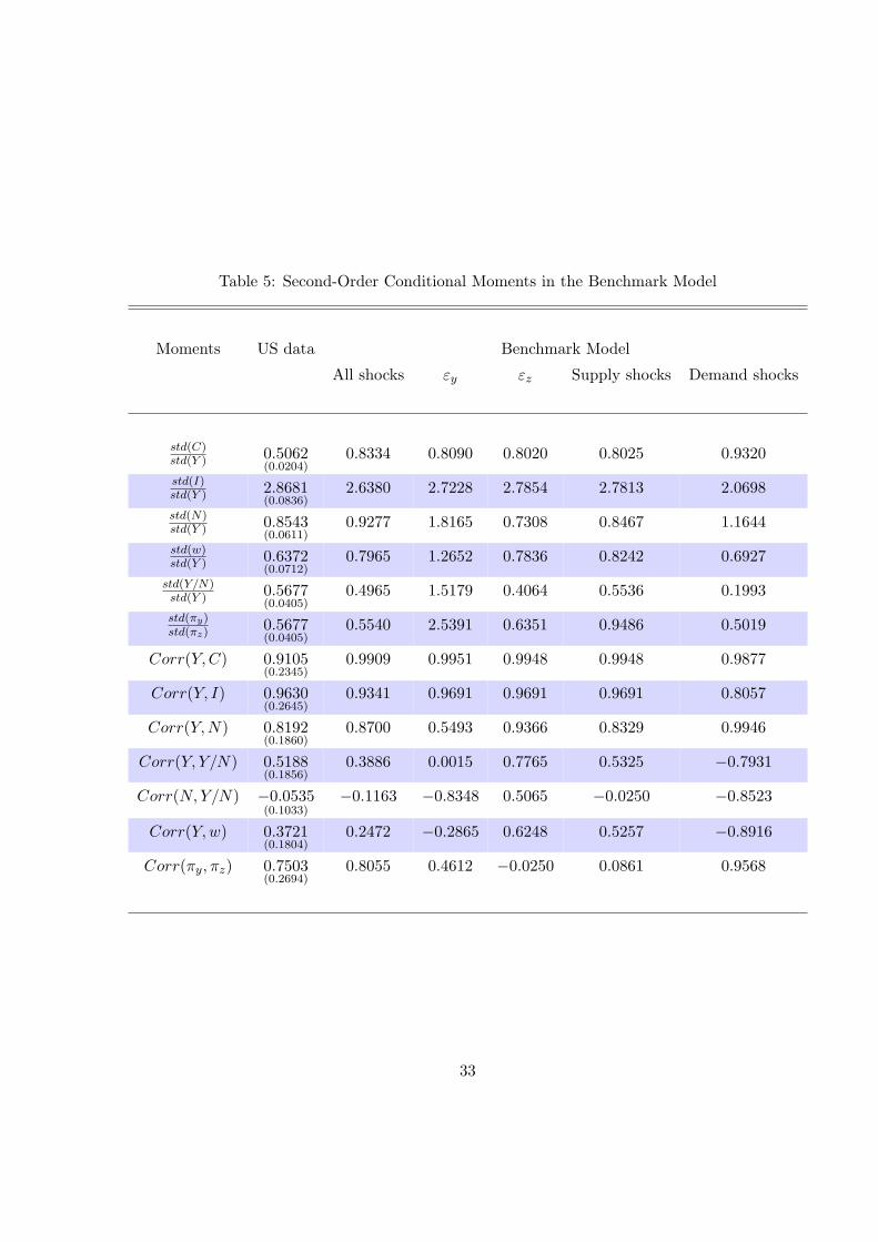
Table 5: Second-Order Conditional Moments in the Benchmark Model
Moments US data Benchmark Model
All shocks εy εz Supply shocks Demand shocks
std(C)std(Y ) 0.5062
(0.0204)0.8334 0.8090 0.8020 0.8025 0.9320
std(I)std(Y ) 2.8681
(0.0836)2.6380 2.7228 2.7854 2.7813 2.0698
std(N)std(Y ) 0.8543
(0.0611)0.9277 1.8165 0.7308 0.8467 1.1644
std(w)std(Y ) 0.6372
(0.0712)0.7965 1.2652 0.7836 0.8242 0.6927
std(Y/N)std(Y ) 0.5677
(0.0405)0.4965 1.5179 0.4064 0.5536 0.1993
std(πy)std(πz) 0.5677
(0.0405)0.5540 2.5391 0.6351 0.9486 0.5019
Corr(Y, C) 0.9105(0.2345)
0.9909 0.9951 0.9948 0.9948 0.9877
Corr(Y, I) 0.9630(0.2645)
0.9341 0.9691 0.9691 0.9691 0.8057
Corr(Y,N) 0.8192(0.1860)
0.8700 0.5493 0.9366 0.8329 0.9946
Corr(Y, Y/N) 0.5188(0.1856)
0.3886 0.0015 0.7765 0.5325 −0.7931
Corr(N,Y/N) −0.0535(0.1033)
−0.1163 −0.8348 0.5065 −0.0250 −0.8523
Corr(Y, w) 0.3721(0.1804)
0.2472 −0.2865 0.6248 0.5257 −0.8916
Corr(πy, πz) 0.7503(0.2694)
0.8055 0.4612 −0.0250 0.0861 0.9568
33

Figure 1: Impulse Responses to an Intermediate-Stage Technology Shock
0 20 400
0.5
1
1.5
Yt
0 20 401
2
3
Zt
0 20 400
0.5
1
Ct
0 20 400
0.5
1
1.5
Nt
0 20 40−0.5
0
0.5
1
Ny,t
0 20 400
1
2
3
Nz,t
0 20 400
2
4
It
0 20 40−1
0
1
2
rkt
0 20 40−0.5
0
0.5
Rt
0 20 40−2
−1
0
pzt
0 20 40−0.5
0
0.5
1
wt
0 20 400
0.2
0.4
Yt/N
t
0 20 40−0.1
0
0.1
πW,t
0 20 40−0.5
0
0.5
πY,t
0 20 40−0.2
0
0.2
πZ,t
34

Figure 2: Impulse Responses to a Final-Stage Technology Shock
0 20 40−0.5
0
0.5
1
Yt
0 20 40−1
−0.5
0
Zt
0 20 40−0.5
0
0.5
1
Ct
0 20 40−1
−0.5
0
0.5
Nt
0 20 40−1
−0.5
0
0.5
Ny,t
0 20 40−1.5
−1
−0.5
0
Nz,t
0 20 40−2
0
2
It
0 20 40−1
−0.5
0
0.5
rkt
0 20 40−0.5
0
0.5
Rt
0 20 400
0.5
1
pzt
0 20 40−0.5
0
0.5
1
wt
0 20 40−0.5
0
0.5
1
Yt/N
t
0 20 40−0.1
0
0.1
πW,t
0 20 40−0.5
0
0.5
πY,t
0 20 40−0.1
0
0.1
πZ,t
35

Figure 3: The Role of the Share of Intermediate Goods, φ
0 10 20 30 40−1
0
1
Yt
Final−goods sector tech. shock
0 10 20 30 40−4
−2
0
Zt
0 10 20 30 40−1
0
1
Nt
0 10 20 30 40−1
0
1
Ny,
t
0 10 20 30 40−4
−2
0
Nz,
t
0 10 20 30 40−1
0
1
c t
0 10 20 30 40−5
0
5
i t
0 10 20 30 400
2
4
pz,
t
0 10 20 30 40−1
0
1
wt
0 10 20 30 400
1
2Interm.−goods sector tech. shock
0 10 20 30 400
10
20
0 10 20 30 400
1
2
0 10 20 30 40−1
0
1
0 10 20 30 400
10
20
0 10 20 30 400
0.5
1
0 10 20 30 400
2
4
0 10 20 30 40−20
−10
0
0 10 20 30 40−1
0
1
solid line: φ = 0.2416; dashed line: φ = 0.0100
36

Figure 4: The Role of Nominal Price Rigidities, dy and dz
0 10 20 30 40−1
0
1
Yt
Final−goods sector tech. shock
0 10 20 30 40−2
−1
0
Zt
0 10 20 30 40−1
0
1
Nt
0 10 20 30 40−1
0
1
Ny,
t
0 10 20 30 40−2
−1
0
Nz,
t
0 10 20 30 40−1
0
1
c t
0 10 20 30 40−2
0
2
i t
0 10 20 30 400
1
2
pz,
t
0 10 20 30 40−1
0
1
wt
0 10 20 30 400
1
2Interm.−goods sector tech. shock
0 10 20 30 400
2
4
0 10 20 30 400
1
2
0 10 20 30 40−1
0
1
0 10 20 30 400
2
4
0 10 20 30 400
1
2
0 10 20 30 400
5
0 10 20 30 40−2
−1
0
0 10 20 30 40−1
0
1
solid line: dy = 0.6561 and dz = 0.6992; dashed line: dy = dz = 0.0000
37

Figure 5: The Role of Nominal Wage Rigidity, dw
0 10 20 30 40−1
0
1
Yt
Final−goods sector tech. shock
0 10 20 30 40−1
0
1
Zt
0 10 20 30 40−1
0
1
Nt
0 10 20 30 40−1
0
1
Ny,
t
0 10 20 30 40−2
0
2
Nz,
t
0 10 20 30 40−1
0
1
c t
0 10 20 30 40−2
0
2
i t
0 10 20 30 40−1
0
1
pz,
t
0 10 20 30 40−1
0
1
wt
0 10 20 30 400
1
2Interm.−goods sector tech. shock
0 10 20 30 400
2
4
0 10 20 30 400
1
2
0 10 20 30 40−1
0
1
0 10 20 30 400
2
4
0 10 20 30 400
0.5
1
0 10 20 30 400
2
4
0 10 20 30 40−2
−1
0
0 10 20 30 40−1
0
1
solid line: dw = 0.8461; dashed line: dw = 0.0000
38

Figure 6: The Role of Labor Adjustment Costs, ϕy and ϕz
0 10 20 30 40−1
0
1
Yt
Final−goods sector tech. shock
0 10 20 30 40−1
−0.5
0
Zt
0 10 20 30 40−1
0
1
Nt
0 10 20 30 40−1
0
1
Ny,
t
0 10 20 30 40−2
−1
0
Nz,
t
0 10 20 30 40−1
0
1
c t
0 10 20 30 40−2
0
2
i t
0 10 20 30 400
0.5
1
pz,
t
0 10 20 30 40−1
0
1
wt
0 10 20 30 400
1
2Interm.−goods sector tech. shock
0 10 20 30 401
2
3
0 10 20 30 400
1
2
0 10 20 30 40−1
0
1
0 10 20 30 400
2
4
0 10 20 30 400
0.5
1
0 10 20 30 400
2
4
0 10 20 30 40−2
−1
0
0 10 20 30 40−1
0
1
solid line: ψy = 5.7406 and ψz = 3.3746; dashed line: ψy = ψz = 0.0000
39