California Center for Population Research On-Line Working Paper Series

Technology and Educational Choices: Evidence from a One-Laptop-per-Child Program

Maria Lucia Yanguas

PWP-CCPR-2018-012

December 9, 2018

Technology and Educational Choices:Evidence from a One-Laptop-per-Child Program

Maria Lucia Yanguas, UCLA∗

December 9, 2018

Job Market Paper

Link to most recent version: www.luciayanguas.com/research

Abstract

Governments and organizations around the globe are seeking to expand chil-dren’s access to computers and the internet as the United Nations calls for effortsto eliminate the digital divide. However, little is known about the effects this ex-pansion may have on long-run human capital accumulation. This paper estimatesthe causal effect of access to computers and the internet on educational attain-ment and choice of major. To establish a causal link, I exploit variation in accessto computers and the internet across cohorts and provinces among primary andmiddle school students in Uruguay, the first country to implement a nationwideone-laptop-per child program. Despite a notable increase in computer access, edu-cational attainment has not increased; however, the program appears to have hadconsiderable effects on other margins. For instance, students who went on to uni-versity were more likely to select majors with good employment prospects. Theywere also less likely to enroll in multiple majors at the same time, thereby reducingcongestion in the public university system.

JEL CODES: I21, I24, I28, H52KEYWORDS: Education Policy, Education and Inequality, Government Expendi-

tures and Education

∗Department of Economics, University of California, Los Angeles. E-mail: myanguas@ucla.edu. Thispaper is the main chapter of my dissertation and my job market paper for 2018/2019. I am especiallygrateful to my advisers Adriana Lleras-Muney, Till von Wachter, Leah Boustan and Michela Giorcellifor their guidance and support. I thank Moshe Buchinsky, Mauricio Mazzocco, Rodrigo Pinto, RicardoPerez-Truglia, Sarah Reber, Manisha Shah, and Melanie Wasserman for helpful feedback. I thank my col-leagues Elior Cohen, Brett McCulley, Bruno Pellegrino, and seminar participants at UCLA, Universidadde la Republica del Uruguay and the Evidence-Based-Economics 2018 conference for valuable comments.This project was supported by the California Center for Population Research at UCLA (CCPR), whichreceives core support (P2C- HD041022) from the Eunice Kennedy Shriver National Institute of ChildHealth and Human Development (NICHD).

1

1 Introduction

Governments around the globe are increasingly concerned about the economic conse-quences of unequal access to technology among school children. One of the targets inGoal 9 of the United Nation’s 2030 Agenda for Sustainable Development is to “signifi-cantly increase access to information and communication technology and strive to provideuniversal and affordable access to the internet in the least developed countries.” One classof programs that has received considerable support and media attention is the one-laptop-per-child initiative, which provides personal laptops to school children and has thus farbeen implemented in at least 42 countries.1

Underlying the adoption of these programs is the idea that broadening access to com-puters among school children will increase their access to learning opportunities anddecrease future inequalities.2 Despite the popularity of these programs, policy evalu-ations of one-laptop-per-child initiatives have found no short-term effects on a set ofsocial, educational, and cognitive outcomes (Beuermann et al., 2015). However, there isno empirical evidence on the overall effects that these interventions may have on long-term human-capital accumulation. As children grow older they become responsible fora larger set of educational decisions, while more years of exposure to computers and theinternet may increase their ability to use technology effectively.

In this paper, I examine the effects of providing laptops with internet access to schoolchildren on their adult educational outcomes. To this end, I use evidence from Plan Ceibalin Uruguay, the first nationwide one-laptop-per-child program, and investigate its effect onchildren’s educational attainment and choice of major one decade after implementation.3

Starting in 2007, Plan Ceibal provided a personal laptop to each student in primary andmiddle schools within the public education system and equipped all public schools withwireless internet access. To the best of my knowledge, this is the first paper to considerthe long-run effects of a one-laptop-per-child program of this scale.

To link participation in the program to children’s adult educational outcomes, I combinesurvey and administrative data from the National Institute of Statistics of Uruguay, theMinistry of Education, and the main universities in the country. In particular, provin-cially representative monthly household survey data (Encuesta Continua de Hogares;1 National partners of the One-Laptop-Per-Child organization include Uruguay, Peru, Argentina, Mex-

ico, and Rwanda. Other significant projects have been started in Gaza, Afghanistan, Haiti, Ethiopia,and Mongolia. In the US, the most famous implementation was OLPC Birmingham (Alabama). Fora review of technology-based approaches in education, see Escueta et al. (2017).

2 The 2017 Measuring the Information Society Report argues that recent advances in technology willenable innovations that have the potential to increase efficiency, productivity, and improve livelihoodsaround the globe.

3 Uruguay is a small country in South America. It was ranked as a high-income country by the UN in2013, with a population of 3.2 million people and a GDP per capita of $19,942 PPP.

2

henceforth, ECH) allow me to track access to technology in the home as well as edu-cational characteristics, and administrative data on all students enrolled in the publicuniversity system allow me to track characteristics of university students and their aca-demic choices.

To identify the causal effect of the intervention, I use information about an individual’scohort and location to approximate their likelihood of being exposed to the program. Thecohorts of older students who were finishing middle school when the intervention arrivedin their province, did not receive laptops, but the younger students did. I therefore usean event-study identification strategy (also called an interrupted time-series) to comparethe educational attainment of individuals who were or were not exposed to the programover time. Identification comes from detecting discontinuities in province-specific trendsaround the first cohort exposed to the program in each province. The most importantassumption is that the province-specific trend up to the first treated cohort is a goodcounterfactual for the outcomes of interest.

I first document that the program was implemented successfully—the rollout was com-plete by 2009 for primary schools and 2011 for middle schools, and essentially everyonewho was targeted received a laptop. I estimate that the program increased students’access to a home computer by 30% (up 20 percentage points from 70% to 90%), whileinternet access in public primary schools more than doubled (up 40 percentage points)between 2007 and 2009.4 The scope and scale of the program make for a great settingin which to conduct this research: if the intervention affects educational outcomes, I amlikely to see it.

I then consider the effects of the program on educational outcomes, starting with ed-ucational attainment. I examine total years of education as well as high school, post-secondary, and university enrollment, and high school graduation rates. Diverse speci-fications show that the program had no effect on educational attainment, especially forpost-secondary enrollment. I estimate that total years of education increased, on aver-age, by only three weeks, a figure not statistically different from zero. To understand thisfinding, I explore the three main reasons for dropping out of high school as reported bystudents: lack of interest in education, finding employment, and, to a lesser extent, be-coming a parent. I find that while most students use the internet for entertainment, veryfew of them report using it for learning activities. Similarly, the program does not ap-pear to have increased employment among adolescents. However, I do find a considerabledecrease in teen pregnancy rates among treated cohorts, which is consistent with bothincreased access to entertainment (and a lesser need to socialize) and increased access to4 Functioning internet connection was available in 26% of public primary schools in 2006 and 70% of

the same schools in 2009. Home computer ownership among school-aged children increased from 35%in 2006 to 90% in December 2009.

3

information about contraceptives and family planning.Next, I investigate whether the program had any effects on choice of major, conditional

on attending university. I use administrative data on all incoming students to Universidadde la Republica, Uruguay’s tuition-free, largely unrestricted public university system,which enrolls over 80% of the country’s university students. According to a recent survey,36% of alumni would choose a different major were they given the chance to go back intime.5 Access to information about the degrees offered and how they are valued by themarket could improve the quality of the match between students and their major.6 Ifind a significant decrease in the fraction of students who enroll in multiple majors at thesame time. This is consistent with the hypothesis that students are more knowledgeableabout the majors and thus have a lesser need to explore by enrolling in multiple fields.This may have important implications for reducing congestion and increasing the qualityof education, which is an important concern in the public university system.

My findings suggest that the reform had some strong effects on the choice of area ofstudy as well, leading students to enroll in majors with good employment prospects. Inparticular, the program was associated with a lower rate of enrollment in the arts andagrarian sciences, and a higher rate of enrollment in health-related majors. Althoughthere are no statistically significant effects on enrollment in social sciences and scienceand technology, the coefficients indicate a relative increase in the latter. Besides access toinformation about employment, these findings could also be explained by computer skillshaving differential returns across courses. Contrary to the information hypothesis, I findthat the fraction of applications for scholarships among enrolled students did not increase.The most common of these scholarships, Fondo de Solidaridad, grants a monthly stipendequivalent to half of a person’s legal minimum income.7

This paper makes three main contributions to the literature. First, this is, to the bestof my knowledge, the first paper to examine the effect of school children’s access to theinternet and personal laptops on their adult educational outcomes. Second, it is the firstpaper to examine the effects of technology access on choice of major. This is particularlycritical in Uruguay, because—unlike in the United States—law and medical degrees areundergraduate options, and thus college majors are better predictors of career choice.Third, this paper exploits a large-scale quasi-experimental design, which addresses theconcerns about external validity from randomized experiments and is particularly relevantfor informing policy.5 Survey run among students who graduated from Universidad de la Republica in 2013. It is consistent

with previous surveys. In addition, 9% of alumnae declared that their major is not related at all totheir current occupation.

6 In addition, there are many vocational tests that students can take on-line.7 http://becas.fondodesolidaridad.edu.uy. This fund is a public organization, created by law in

1994, and its task is to provide scholarships for post-secondary education in public institutions.

4

Due to the popularity of these interventions and newly available data, there is nowabundant evidence on the short-term effects of computers on learning in primary andsecondary school. De Melo et al. (2014) analyzed Plan Ceibal’s influence on primaryschool math and reading scores two years after the intervention and detected no effects.Their finding is in line with other papers. In a small-scale implementation in Peru thatused the same devices, Beuermann et al. (2015) found no effects on academic achieve-ment or cognitive skills in the short run, although lower academic effort was reportedby teachers. They found short-run improvements in proficiency at using the program’scomputer (which typically runs Linux) but no improvements in either Windows computerliteracy or abstract reasoning. A greater concern is that some studies found negative ef-fects on academic achievement from interventions that are purely focused on expandingtechnology access (see Vigdor et al., 2014; Malamud and Pop-Eleches, 2011), contrastingwith positive effects found in alternative programs that use technology specifically foreducational purposes (see Banerjee et al., 2007; Roschelle et al., 2016). This suggeststhat the effects of technology are likely to vary depending on how children use it.8

A few papers have examined the effects of access to technology at more advancedstages of the education system. For instance, Cristia et al. (2014) find no statisticallysignificant effects of high school computing labs on grade repetition, dropping out, andinitial enrollment in Peru between 2006 and 2008, ruling out even modest effects. Det-tling et al. (2015) examine effects of high-speed internet access in early adulthood oncollege-entry examinations and college applications. They find that while broadbandaccess generally increased applications to college, the effects were concentrated amonghigh-income students. They worry that new technology may be increasing preexistinginequities. Fairlie and London (2012) studied the effects of donating laptops to recentlyenrolled community-college students on their academic performance. They found someevidence that the treatment group achieved better educational outcomes.

In sum, the literature has typically found very small effects on academic performance,with results ranging from negative to positive depending on the educational level of therecipient. This is consistent with the hypothesis that results depend on the computers’ in-tended use. College students are likely more inclined—either by nature or by context—touse computers for educational purposes. In a follow-up to the community-college experi-ment (Fairlie and Bahr, 2018), the authors matched students to employment and earningsrecords for seven years after the random provision of computers.9 They found no evi-dence that computers have short- or medium-run effects on earnings or college enrollment.However, for many reasons, giving computer access to adults is likely to be different from8 This is influenced by the level of parental supervision and teacher engagement.9 This was the first study, to my knowledge, to have looked at medium-run effects of a one-to-one

computer program on employment and college.

5

giving it to children. Besides developmental considerations (see Heckman 2006; Doyleet al. 2009) and the likely presence of an experience-curve (see Van Deursen et al., 2011)for computer and internet skills, the effects of technology access on later-life outcomessuch as income may operate through channels that happen earlier in life such as highschool enrollment, graduation, and career choice.

The direction of the effect of technology access on educational choices is not obvious. Forinstance, internet and computer access in schools might make the educational experiencemore enjoyable to children and may allow teachers to adapt more effectively to eachstudent’s level and needs. On the other hand, access to entertainment may encourageleisure and drive students to pay less attention in class. This can in turn affect students’daily decisions about whether to attend class and how much effort to put forth, as well asdecisions with long-lasting effects such as whether to enroll or drop out of school. In thelonger run, prolonged exposure to information technologies might affect the way studentslearn about the costs and benefits of college and career choices. Moreover, technicalskills may be more valuable in college than in primary and secondary school (see Escuetaet al., 2017), and awareness of this may reduce the expected costs of attendance. Similarly,computer access may also affect students’ career choices, by encouraging them to pursuecareers that are more likely to involve or require computing technology. On the otherhand, computer skills that are valuable in the labor market may discourage children fromfurthering their education.10

The rest of this paper proceeds as follows. Section 2 describes the program. Section 3describes the data and summary statistics. Section 4 outlines the identification approachand technical details of the implementation. Section 5 presents the results. Section 6considers intermediate outcomes. Section 7 concludes.

2 The One-Laptop-Per-Child Program in Uruguay:Plan Ceibal

One Laptop per Child (OLPC) is a nonprofit initiative founded in 2005 by MIT professorNicholas Negroponte. Its mission is to empower the children of developing countries tolearn by providing one internet-connected laptop to every school-age child. The organi-zation creates and distributes educational devices for the developing world and createssoftware and content for those devices. One-laptop-per-child programs have been imple-mented in partnership with the OLPC organization in at least 42 countries.10 This includes searching for jobs in the Internet, networking, writing an acceptable CV, etc.

6

2.1 Implementation

In 2007, in partnership with OLPC, the government of Uruguay launched Plan Ceibal,an ambitious program designed to eliminate the existing technological gap between pri-vate and public school students. Plan Ceibal provides laptops with wireless modems tostudents and teachers in public primary schools, middle schools, and teacher training in-stitutes. As of December 2016, 1.6 million laptops had been deployed, enough to doublethe number of children under 15 years old living in the country.11

Plan Ceibal was implemented in two phases, each lasting three years (see Figure 1).Within any province, each primary school was equipped with wireless internet access.Once internet access reached the 90% threshold, Plan Ceibal handed out a personalcomputer to each primary school student enrolled in that province’s public educationsystem. Uruguay has 19 provinces. One (Florida) entered the program at the end of2007; sixteen entered in 2008; finally, Canelones and Montevideo (where 40% of thepopulation lives) entered at the start of 2009. This three-year gap in the timing of theprogram yields three cohorts of students whose exposure to the program during primaryschool depended on their place of residence. Laptops were initially lent to these students;by design, they could take full ownership of their laptop upon completing primary school.Between 2007 and 2009, 380,615 laptops were provided in primary schools.12

Phase 2 focused on secondary schools. In 2009, the pilot program was implementedin the province of Treinta y Tres, in which all students in middle school (grades 1, 2,and 3 of secondary school) received Windows laptops (donated by Microsoft), and morethan 90% of the province’s schools were equipped with wireless internet access. In 2010,after the implementation of this pilot was deemed successful, the rollout was extendedto grade 2 students in the provinces of Montevideo and Canelones. In 2011, the rolloutwas extended to the rest of the country. At this point, the program was tasked withreplacing the primary school laptops with newer laptops equipped with software that wasgeared towards middle school students. As with the primary school program, laptopswere initially lent to students, who could take full ownership of them after completingmiddle school. In addition, from 2010 to 2014, some public high school students (grades4 and 5 of secondary school) who had entered the technological track rather than theregular track—about 10% to 15% of all high school students—also received laptops. Thisadjunct program ended in 2014 due to financial constraints. In all, between 2009 and2011, 134,111 laptops were provided in secondary schools.11 This number represents almost half of the entire population in 2016 (3.4 million). The explanation

is that children would get two laptops in their lifetime: one in primary school and a different one inmiddle school, at which point the first laptop would go back to the state. Moreover, broken laptopshad to be replaced.

12 As a reference, 292,900 students were enrolled in public primary schools in 2009.

7

Official data provided by Plan Ceibal shows that by June 2010, 98% of primary publicschools and 90% of public middle schools in the country had wireless connection. Publicprimary school census data from the Ministry of Education of Uruguay (ANEP) allowsme to verify that internet connectivity increased significantly during the expansion periodof the program. That data shows that functioning Internet connection was available in26% of public primary schools in 2006 and 70% of them in 2009.13

Plan Ceibal was implemented successfully. Using data from Uruguay’s monthly house-hold survey (which I describe in more detail below), I track the fraction of individualsaged 6 to 15 who reported having a computer in their home: It increased 25 percentagepoints (from 50% to 75%) in the quarter in which the program was implemented in theirprovince, and 40 percentage points (50% to 90%) when compared to the following quarter(Figure 2, Panel A).14 Compellingly, there was no change at all around that time-framein computer access for adults living with no children. Computer access among publicschool students had increased by 150% only two years after the intervention—I estimatean increase close to 90% in the first quarter of implementation alone (Figure 2, PanelB).15 In effect, this increased access benefited only public school children; those enrolledin private schools experienced no significant discontinuities in computer access aroundthat date.

Using the same data, Figure 3 shows variation in computer access across cohorts ofindividuals in a cross-section of 2011. Panel A shows that access to a government laptopat home was around 60% among treated cohorts up to five years after deployment; PanelB shows that essentially all public school students had laptops, in striking contrast toprivate school students. Panels C and D show that this resulted in a 40% increase incomputer access among all individuals in the relevant cohorts and a 50% increase whencomparing public to private school students.13 See Web Appendix [Figure 2].14 The specific question as it appears in the household portion of the survey is: does this home have a

personal computer?The informant is a member of the household (excluding domestic service) over 18years old, mentally capable, who can provide information about the home and rest of the householdmembers. An individual is said to have reported a computer at home whenever the household informantreports a computer.

15 The ECH survey does not provide data on school type for the years 2009 and 2010. To address this,I replace public school computer access by the average access in the student population, which is inits majority public sector. In the rest of the country, for which I do have data immediately after theintervention, the immediate increase in computer access was indeed about 90%.

8

2.2 The Computer

Plan Ceibal equipped each student with an XO-1 laptop, a small, durable, efficient, low-cost laptop that functions much like a normal PC.16

Reviews found in the internet tend to converge to one conclusion:

“The XO-1 won’t ramp up your digital productivity or amaze you with hi-def visuals. But (...) it celebrates its ability to communicate with peoplearound the corner or around the world, access information, design programsand manipulate music, sound or pictures.”17

The laptop features 128MB of RAM, 1GB of NAND flash memory (instead of a harddisk), a 7-1/2-inch dual-mode LCD, wireless networking, and a video camera. It’s alsodesigned to be operated by children and is therefore durable and rugged. In additionto a standard plug-in power supply, human power and solar power sources are available,allowing it to be operated far from a commercial power grid. The wireless technologysupports both standard and mesh networking, which allows laptops to network peer-to-peer, without the need for a separate router. The XO-1 uses a GNU/Linux operatingsystem, and all its software is free and open source. It comes with basic software installed.Plan Ceibal reported in 2009 that among schools with connectivity that used the laptopsin class, 90% of students navigated the internet, 60% used the writing software, and15% used the drawing software, with smaller percentages using the calculator, chatting,reading a book, and memorizing concepts.18

Pricing for the XO was set to start at US$188 in 2006, with the goal to reach the $100mark in 2008. When the program launched, the typical laptop retailed for well north of$1,000.

2.3 Cost and Financing of the Program

As of December 2016, 1,681,830 devices had been dispatched by the program.19 At $188per laptop, this would imply a direct cost of about $300 million. However, the overalloperational costs of Plan Ceibal were higher, about $500 million by 2017. As a reference,16 The display is the most expensive component in most laptops, so the development of a new,

cheaper display was instrumental to the creation of the XO. See http://wiki.laptop.org/im-ages/7/71/CL1A_Hdwe_Design_Spec.pdf for more details.

17 National-level programming competitions using the XO laptops began in 2010. There are severalaccounts of children creating/developing games in these laptops. While this does not mean the practicewas universal, programming was certainly possible. See https://www.cnet.com/uk/products/olpc-xo-1-one-laptop-per-child/review/2/.

18 https://www.ceibal.edu.uy19 This number includes laptops and tablets. Source: Memoria Explicativa de los Estados Contables al

31 de Diciembre de 2016, Centro Ceibal.

9

this equates to an average of 3% of Uruguay’s annual education budget and 0.4% ofits annual federal budget since 2007.20 The ultimate cost of the program added up toapproximately $600 per student.21

The program was financed mostly with taxpayer money, as Plan Ceibal got its ownportion of the federal budget. There is no evidence that this implied a decrease in ex-penditures in other areas of education—in fact, the economy was growing and the overalleducation budget was rising. The Inter-American Development Bank helped finance theprogram through two loans: $5 million in 2010 and $30 million in 2017.

3 Data and Summary Statistics

In this study, I combine three datasets: (1) the 2001–2017 household survey data (ECH),which contains information on technology access and education; (2) tabulated enrollmentdata from 2001 to 2016 from the Ministry of Education and private universities, by year,province of origin, gender, and school type; and (3) administrative data from 2006 to2016 for all 208,946 entering students in the public university system (Universidad de laRepublica), which contains information about major of choice.

3.1 Data Sources

My main data source is the 2001–2017 Uruguay Continuous Household Survey (En-cuesta Continua de Hogares; henceforth, ECH), which samples about 3.5% of particulardwellings each year.22 This publicly available monthly survey comprises independentcross-sections, representative at the provincial level. It provides standard information oneducation and labor-market outcomes. The questionnaire has been continually revisedover the last two decades, which has allowed for the timely incorporation of novel ques-tions, including some on technology ownership and use (for example, the presence of acomputer and/or the internet in the house). Moreover, since 2009 the questionnaire hasincorporated a specific question about ownership of a laptop from Plan Ceibal. The sur-vey also collects the number of years of education (attended and/or completed). Otheruseful variables include the type of primary and middle school institutions attended (pub-lic or private) and years of age, together with year and month of the survey. Moreover,questions about migration are included as well: Since 2007, the survey has been asking20 From official Ceibal Financial records 2010-2016, the Institute of Statistics and the Government Budget

2006 and 2008.21 With 429,016 students enrolled in public primary and middle school in 2007 and assuming the number

of students would have exactly duplicated by 2016.22 ECH stands for Encuesta Continua de Hogares. The sample size was half this figure before 2006.

Estimate based on the 2004 and 2011 Census of Population and Dwellings.

10

about the province of birth, and since 2012 it has asked about the province of residencefive years prior.

The household survey data is very convenient. Its main virtue: it allows me to estimatethe effect of the program on computer access (as was demonstrated in Figures 2 and3). However, it contains only a small sample of the population. Therefore, for thepurpose of checking the robustness of my results, I also collect aggregate data on thepopulation as a whole from the Ministry of Education. I collect tabulated enrollment databy calendar and academic year, province of school location, gender, and school type. Dueto migration concerns, – most of these educational establishments are in Montevideo; Icannot use this same data for postsecondary enrollment. Therefore, I also contacted eachuniversity in Uruguay to collect tabulated data on their student demographics, includingyear of enrollment and province of origin in the 2010–2016 period. My resulting sampleencompasses more than 95% of university students in Uruguay.23

To examine how the program affected choice of major, I obtained access to restrictedadministrative data on 208,946 incoming students to the Universidad de la Republicabetween 2006 and 2016. This is the nation’s largest university, attended by more than80% of its university students. This dataset contains the specific majors chosen by theindividual as well as their exact province and date of birth, year of high school graduation,location of primary and secondary school, and whether those were in the private or publicsystem. It also contains information on whether the child applied for financial aid or hadto move to study a specific major, as well as several individual and parental characteristics.

Finally, in order to verify the expansion of internet access around the start of PlanCeibal, I collect data on the availability of internet access at schools from the annualcensus of public primary schools, which was conducted by ANEP from 2002 to 2009.24

3.2 Summary Statistics

In the Web Appendix [Table 2] I show summary statistics for individuals aged 18–20 in2011 to 2017 using the household survey data. Approximately half the sample is male,and one out of five individuals is nonwhite. In terms of socioeconomic status, one out often lives below the poverty line, and 42% claim to be employed.25 The average individualin this age group lives in a four-person household, and four out of five individuals stilllive with their parents or grandparents. In addition, almost one out of five women have23 The sample includes the following universities: Universidad de la Republica (public), Universidad de

Montevideo (private), Universidad Catolica del Uruguay (private), Universidad ORT (private).24 This information was not available in the web, I learned about it through an interview with the director

of the research department in ANEP, who then had the data processed and sent to me.25 This is comparable to the US average for the entire population.

11

children.26

In terms of access to and use of technology, four out of five individuals have a computerat home, three out of five have a regular (non-government) computer at home, and threeout of five have internet access at home. In-home computers are usually shared: there isabout one computer for every two persons in a household. Overall, 75% used a computerin the month prior to the survey, and 64% reported using the internet every day (thisis consistent with the fact that only 42% of individuals age 15 to 20 had a smartphoneat home in 2013).27 Internet use is spread evenly between entertainment, information,and communication (about 30% each), while about 10% is for education or learningactivities.28

In terms of education, the public sector is very large: 85% of people who ever enrolledin primary school, middle school, or university did so in a public institution. Educationalattainment is lower in Uruguay than in the United States, the OECD, and Latin Americaand the Caribbean. The average years of education (completed) among individuals aged18 to 20 is 9.9; only 60% ever attended a high school, and only 29% ever graduatedfrom high school. Among the reported reasons for dropping out of secondary school,lack of interest (55%) tops the list, followed by starting to work (20%), pregnancy (7%),and finding classes difficult (7%).29 Moreover, 12% attended technical school and 4%graduated from it. With respect to higher education, only 21% enrolled in any postsec-ondary education and only 18% enrolled in university. Finally, a considerable gap existsbetween public and private school students. Public school students have on average 9.7years of education by age 20; private school students have on average 11.86, and almostall of them enroll in high school. Therefore, a large opportunity exists for increasingeducational attainment.

4 Identification Strategy

This section outlines my empirical approach to identifying the causal effect of the one-laptop-per-child program.26 Adolescent births in Uruguay are well above the global average. According to World Health Orga-

nization, in 2015 4.7% of teenage women (age 15 to 19) had children globally, compared to 8.8% inUruguay, which ranked right in between the averages for West Africa (11%) and Latin America andthe Caribbean (6%).

27 This question is not included in ECH. This data comes from the nationally representative EUTICsurvey made in 2013.

28 See Web Appendix [Figure 5].29 See Web Appendix [Figure 5].

12

4.1 Empirical Specification

To estimate the effect of the one-laptop-per-child program I implement an event-studyidentification strategy (also called an interrupted time-series) that compares educationaloutcomes of individuals who were or were not exposed to the program over time. Thus,identification comes from detecting discontinuities in province-specific trends around thefirst cohort exposed to the program in each province. The most important assumption isthat the province-specific trend up to the first treated cohort is a good counterfactual forthe outcomes of interest. The key idea is that students who were already in high schoolwhen the program arrived in their province did not receive a laptop, but those who werein primary school would eventually receive one.

I start by documenting that school grade is a very precise indicator of whether anindividual has a government laptop within one year of the intervention in any givenprovince. By combining the primary and middle school interventions in each province, Iverify that the oldest students to enter the program in Treinta y Tres were enrolled in9th grade in 2009, while the oldest students to receive the intervention in Florida wereenrolled in the 6th grade in 2007 (expected to be in 9th grade in 2010), and the oldestones to enter the program in the rest of the country were enrolled in 9th grade in 2011.Hence, there is a one year gap in access to the program between Treinta y Tres andFlorida, and between Florida and the rest of the country (see Web Appendix Table 1 formore details). In turn, this gap in access to the program across school grades (which isnot easily observable for adults) extends across birth cohorts (which I can observe in mydata): the oldest students to be exposed to the program in Florida and Treinta y Treswere on average one and two years older, respectively, than students in the rest of theprovinces.

In my analysis I focus on adults, and I have no information about the school grade theywere enrolled in back when the program arrived in their province. Therefore, I must relyon their cohort of birth to classify individuals into those who were or were not exposedto the program. Birth cohorts are imperfect indicators of who received a governmentlaptop in a given province because repetition rates are relatively high. However, I amable to observe the exact relationship between birth cohorts and school grade throughthe years, which allows me to track the exact proportion of treated individuals in eachcohort. Based on this, I classify cohorts into those who were fully exposed to the program,those who were not exposed to the program, and those who were partially exposed to theprogram.

Figure 3 tracks the variation in access to computers across cohorts and provinces.Panel A shows the fraction of individuals (with no younger siblings) with a government

13

computer at home in 2011 (up to five years after the rollout) stacked by province. Iclassify cohorts into three groups within each province as a function of their degree ofexposure to the program: (1) “after-intervention” cohorts, those with more than 60%access to a government computer at home in 2011; (2) “before-intervention” cohorts,those who were not exposed to the program and had virtually no government computersat home; and (3) “in-between” cohorts, those who were only partially exposed to theprogram in their respective provinces, with 10%–25% access to a government computerin 2011.30 As mentioned above, partial exposure is the result of some individuals laggingbehind in school for cohorts that would otherwise be classified as “before-intervention”cohorts (see the Web Appendix Figure 3 for more details).

To estimate the effects of the program on adult educational outcomes, I concentrateon individuals born between May 1988 and April 1998 and estimate the following regres-sion:31

Yisc = α + ηs + γsTrendc + β(In - betweensc) + θ(Aftersc) +X′iscΓ + εisc , (1)

where Yisc is the outcome of interest measured around age 19 for every cohort, i indexesthe child, s indexes the province, and c indexes the year in which the child was expectedto start primary school. The vector of covariates Xisc includes individual-level character-istics such as exact age, race and gender fixed effects to make the estimates more precise;and family income and parental education to try to control for province-specific trends.32

The dummy variable In - betweensc is equal to one for cohorts in the partially treatedgroup within each province: students born between May 1994 and April 1996 in Treintay Tres, May 1995 and April 1997 in Florida, and May 1996 and April 1998 in the rest ofthe country. The dummy variable Aftersc is equal to one for cohorts in the treatmentgroup within each province: students born from May 1995 onward in Treinta y Tres,from May 1996 onward in Florida, and from May 1997 onward in the rest of the country.The regression includes province fixed effects and province-specific time-trends meant tocontrol for potential differential trends across provinces. The parameter of interest θ

captures the average causal effect of receiving a personal computer with internet access,for children of primary and middle-school age, after the program.

I interpret θ as an intent-to-treat effect, since the regression model estimates thereduced-form effects on all children from post-reform cohorts in each province. This30 A similar strategy was used in Havnes and Mogstad (2011).31 In the ECH survey I do not have date of birth, but I estimate it based on the age of the child in the

month and year of the survey.32 Since the ECH survey does not report parental characteristics for individuals who are no longer living

with their families, whenever I use this survey I use average household income and parental educationshares for individuals residing in the province were each adult individual was living 5 years ago, ataround age 11.

14

specification does not capture the potential effects of the program on older cohorts ofstudents, who may have been induced to purchase laptops or may have benefited fromthe laptops of younger relatives, neighbors and friends. As a robustness check, I alsoreport the results of this specification where the In-between cohorts are dropped out ofthe sample within each province (sometimes called “doughnut” sample).33 My results arerobust to this change.

4.2 Alternative Specification: Exploiting School Type

Besides province and cohort, school type is the third dimension along which the treat-ment varies. This approach considers this additional source of variation, assuming thatwhatever changes are observed among private school students are caused by other factorsand that this group can provide a counterfactual trend. To exploit this additional sourceof variation, I implement the difference-in-differences strategy specified below:

Yiscp = α + γsTrendc + φPublicp + δ(In - betweensc) + κ(Aftersc) +

β(Publicp ∗ In - betweensc) + θ(Publicp ∗ Aftersc) +X′iscpΓ + εiscp , (2)

where Publicp is an indicator for individuals who completed the majority of their primaryor middle school education in the public system. Including a comparison group who isnever treated even among post-treatment cohorts is useful given that all provinces areeventually treated. For the treatment effect on private school students to serve as abenchmark, it’s necessary to assume that public school students would have experiencedthe same trend in educational outcomes as private school students in the absence of theintervention. On the other hand, private and public school students are very different(private school student typically have higher income and more educated parents), andit’s not clear that they would experience parallel trends. Another concern is that privateschool students may have been indirectly affected by the program, which, if true, wouldbias my estimates towards zero. Since most of the private-school population resides inMontevideo, and for a differences-in-differences specification I need sufficient private-school observations in each province, I limit the sample to Montevideo residents for thisspecification. My results are reported in the Web Appendix; they are very similar to theones obtained with the main specification.33 Since the treatment effects of the program show some heterogeneity across provinces, the difference-

in-differences estimate is hard to interpret and generalize to the entire population which is why I donot follow that identification strategy.

15

4.3 Threats to Identification

In this section I discuss two threats to identification. First, exposure of the older cohortsto the program could generate a bias toward zero. This is likely to arise if there iserror in assigning individuals to their correct province or cohort. Second, any unobserveddifferences between older and younger cohorts, when not captured by a linear trend, couldbias the estimates. This is likely to arise if the post-treatment cohorts where alreadydifferent at the baseline or experienced differential shocks before age 19. A third threat,which I will not analyze here, would be functional form: a non-linear pre-trend could biasmy results either way. I deal with this directly on the robustness checks section.

4.3.1 Cohort Assignment

My analysis relies heavily on my ability to distinguish between before- and after-interventioncohorts and their “distance” from treatment. The ideal way to classify individuals into co-horts would be to know exactly the school grade they were enrolled in when the programreached their province. This information would obviate the need for partially treated(“in-between”) cohorts. Unfortunately, this information is not available in any of mydata sources. In this subsection, I explain how I classify individuals into cohorts furtherfrom or closer to exposure to Plan Ceibal, and I show how my treatment of in-betweencohorts addresses the concerns of attenuation bias.

The best way to estimate students’ date of exposure is to use their high school grad-uation year. The university individual-level data provides this information for selectedyears (2011–2016), which allows me to backtrack the correct cohort under the assump-tion of no grade repetition in secondary school. Because I use this dataset only to testhypotheses among college students, this strategy is convenient. Repetition in Uruguay isnot negligible. Almost 20% of students repeat grade 1, and only 40% of students enrolledin grade 12 in 2011 were in the correct age for the grade. But, conditional on startingmiddle school, 75% of students reached grade 12 at the expected time. Unfortunately,high school graduation years are not available for the entire period, nor are they in myother datasets. In addition, using the year of high school graduation to estimate effectson educational attainment would be problematic.

Instead, I can use students’ date of birth and assume that children start primary schoolat the compulsory starting age to determine their grade at the time of the program. InUruguay, children can begin primary school if they are at least 6 years old in March orturning 6 by the end of April. There is evidence that the regulation is respected: allstudents enrolled in the first grade of primary school in 2006 were at least 6 years oldby April 30. Moreover, this age group represented more than 66% of entering students

16

and an estimate based on the age law is the best predictor of being enrolled in grade 1conditional on primary school enrollment.34

Because date of birth is not available in the ECH survey, I use information on age,month, and year of observation to determine a student’s probability of being 6 yearsold by April of a given year, under the assumption that births are uniformly distributedacross the year.35 For observations occurring in October, the probability of being in onecohort or the following one is exactly 50%. For this reason, I eliminate that month frommy dataset when using this method and classify individuals in the cohort for which theprobability surpasses 50%. This way, misclassification error stays well below 25%.

My methodology works well: about 80% of students who I classified in second gradewere indeed enrolled in second grade. However, only about 50% remained enrolled in theright grade for their cohort by the end of middle school, which suggests that repetitionis a non-negligible concern. I address this concern by identifying an in-between groupin the analysis. In-between cohorts are those that would have never been exposed tothe intervention if it weren’t for the fact that a fraction of them were enrolled one ortwo years behind their age in school in their respective province. My empirical approachtreats these cohorts differently (and even drops them) to ensure that my estimate is notbiased toward zero.

Finally, even with a perfect cohort assignment, there could be a bias toward zero forindividuals with younger siblings (50% of students have younger siblings aged 5 to 18at home). Because students are encouraged to take their laptops home, treated siblingscould affect their relatives. Even if this is not the case, younger siblings can be a problemwhen estimating the effect of the program on the presence of computers at home, whichis why I limit the sample to individuals with no younger siblings aged 5 to 18 in theirhousehold.

4.3.2 Province Assignment

My analysis also relies on my ability to classify adults in their province of residence atthe time of the intervention. Ideally, I would like to know the exact province in whicheveryone attended primary and middle school. Unfortunately, I have this informationonly for a limited number of years and only for the university microdata. For the otherdata, I must decide between province of birth, province of residence, and province ofpast residence. Misclassification error is likely to create a bias toward zero. But the biascould go in either direction if migration was differential by treatment. If, for example,34 From the Ministry of Education of Uruguay. Refer to Web Appendix [Table 3] for more details.35 This simplifying assumption is supported by the Vital Statistics shown in the Web Appendix [Table

2].

17

treated cohorts from the least developed provinces were more likely to migrate to thericher provinces than the previous cohorts, the effects might be downward biased.

However, Uruguay is a highly centralized country—more than 40% of the populationand educational opportunities are concentrated in Montevideo. Hence, cross-provincemigration exists and is likely to be correlated with educational choices. Using householdsurvey data, I find two clear trend breaks in migration patterns by age. The probability ofmoving out of the province of birth is high before primary school (ages 0 to 5), plummetsduring formal education (ages 6 to 17), and spikes again after high school (ages 18–20). Bythe time they start primary school, 6% of students have already moved outside their birth-province; this percentage rises to 11% during the last year of high school and almost 15%at age 19. This trend suggests that individuals move to study or work after completingtheir formal education.

Since migration out of province of birth is already non-negligible by the start of primaryschool, my strategy for dealing with migration is to use the previous province of residencewhen measuring outcomes among adults and to use province of current residence whenmeasuring outcomes among children. I also conduct robustness checks using province ofbirth (this information is available in all my datasets.) Cross-country migration is also apotential concern, but I will not be able to account for it in my data.36

Finally, in one of my specifications I limit my dataset to Montevideo neighborhoods.Here migration is less of a concern, because treatment status does not depend on theneighborhood of residence, and because migrating for school of work is less necessary.37

In 2011, the ECH survey included questions about cross-neighborhood migration, andI can check that in the sample of 18-year-old students who declared to have lived inMontevideo five years prior and still live in Montevideo today, 83% lived in the sameneighborhood five years prior. The share of students living in the same neighborhoodas five years prior is a bit higher among private school students relative to public schoolstudents: 92% vs 80%.

4.3.3 Differences Between Older and Younger Cohorts

Any unobserved differences between older and younger cohorts, when not captured by alinear trend, could bias the estimates. This is likely to arise if the treated cohorts werealready different at the baseline or experienced differential shocks before age 19.

Figure 4 shows that there were no variations from trend at the baseline (age 11; 6th36 Net entries to the Carrasco Airport were increasing up to 2013, after which the trend reverts (net

emigration represented 0.4% of the population in 2015). Unfortunately, the migration office is not ableto separate this by age groups.

37 Montevideo is small enough that it can be crossed from side to side in 1 hour by car, and has goodpublic transport.

18

grade) for a set of observable characteristics in the period 2001-2014. Each scatter plotindicates the average value of an outcome according to distance from treatment in aprovince, while the dashed dashed line is designed to be a linear fit for the cohorts thatwill never be exposed to the intervention in each province. Clearly, there are no significantvariations from this linear trend among years of education, public school students, teacheremployment, TV subscriptions or parental education. Economic conditions, which gen-erally vary over time, are a clear threat to identification. Household income appears toexperience an upward change in trend for younger cohorts that are completing primaryschool. This trend-change is not statistically significant, but I will give it special atten-tion in the robustness section. In the Web Appendix, I show a similar figure for 2006,where household income is similar across all cohorts. I also plot household income acrosscohorts for every age 11 to 19, to check that there were no obvious trend breaks at thosecritical ages (despite the 2016 economic downturn).

In Table 1 I estimate equation 1 for predetermined covariates and expect to find noeffects. Panel A shows the regression results for 13 observable characteristics measuredat age 11 (including the ones discussed above). As expected, none of these characteristicsdeviates significantly from trend. It is especially important to mention that there is nosignificant deviation from the trend for treated cohorts in employment or income amongteachers when students are around age 11. This is key for interpreting my results: it meansthat the program is not significantly affecting the income or quantity of teachers, whichwas a potential concern. Panel B focuses on observable characteristics in 2006—the yearbefore the program was implemented—when students of different cohorts have differentages. No significant difference exists among students in internet access at home, havinga mobile phone, government aid, household income, or the fraction of racial minorities.The only difference is that, if anything, treated cohorts (that were younger in 2006) wereabout 15% less likely to have a computer at home. But non-linear trends in ownershipof technology across ages are present for all years before the start of the program.

4.4 Inference

According to Abadie et al. (2017) there are two justifications for clustering standard er-rors: (1) clustered sampling and (2) clustered treatment assignment. None of my datawere collected through clustered sampling. However, the treatment status was assignedat the province level for all individuals in public schools, rather than randomly acrossindividuals. Thus, clustering at the province level is indeed warranted by experimentaldesign—even after including province fixed effects—as treatment likely had heterogeneouseffects across clusters. Given heterogeneity in the size of clusters, I should also run re-gressions at the cluster level to check robustness (see Athey and Imbens, 2017). I present

19

these additional specifications in the Web Appendix. Moreover, standard errors shouldbe clustered at the treatment level, which in this case can be thought of as the provinceor province by school type. The trade-off between the two is that while high-order clus-tering typically has lower bias, lower-order clustering produces more precise estimates ofthe variance. Moreover, with province-level clustering, the validity of clustered standarderrors is reduced because I run into the problem of having few clusters (19 provinces).When clustering at the province level, I address this by reporting p-values from province-clustered wild-bootstrapped t-statistics. This method has been shown to work well inCameron et al. (2008), but MacKinnon and Webb (2017) show that wild-cluster boot-strapping severely under-rejects when the fraction of treated clusters is either very largeor very small.

Alternatively, I can avoid the question of clustering completely and produce inference byrandomization or permutation tests. The advantage is that these tests do not depend onassumptions about the shape of the error distribution. They work by shuffling the timingof the treatment in each province, generating placebos. I conclude that my findings arestatistically significant only if they would have been very rare under a random assignmentof the program. In this paper, I report p-values generated from permuting treatmentassignment among provinces and cohorts. My chosen approach leaves fixed the numberof provinces treated for each cohort and permutes only the order in which provinces aretreated, following Wing and Marier (2014). I go over all the potential combinations ofprovinces—342 repetitions in all.38

5 Results

I first show that the intervention increased ownership of computers in the targeted pop-ulation, using information on the presence of a computer in the house from the monthlyhousehold survey in 2011.

I start by estimating equation 1 in a sample of nine cohorts of individuals living with noyounger siblings – I use seven cohorts by province to guarantee three pre-intervention andtwo post-intervention cohorts in each province – in 2011. Panel A in Table 3 shows thatthe intervention increased access to a computer in the house among treated cohorts byabout 17 percentage points (23%). Panel B estimates equation 1 in a doughnut samplethat excludes the in-between cohorts in each province and the estimate is essentiallyunchanged. Results are significant at 1% level with and without controls, with robust and38 I also conducted robustness checks in which I cluster by cohort (not reported), which does not affect

the interpretation of my results. I plan to produce estimates using the Newey–West estimator, whichis used to try to overcome serial correlation (when the error terms are correlated over time) andheteroskedasticity in the error terms for regressions applied to time series data.

20

province-clustered standard errors, as well as with a p-value computed from a permutationtest of treatment assignment and a province-clustered wild bootstrap. This trend-breakis significant in each province (see Web Appendix).

5.1 Educational Attainment

5.1.1 Summary Statistics

I start with background information on educational attainment in Uruguay. Accordingto ECH data from 2015, only 56% of individuals aged 25 to 34 had at least some highschool education, and only 39% had completed high school. Only 21% had at leastsome postsecondary education, and just 9% had earned a postsecondary diploma. At theuniversity level, the numbers were even smaller: only 13% had any university education,and only 5.6% had earned an undergraduate degree. Clearly, there is ample marginto improve educational attainment in Uruguay. Moreover, Universidad de la Republicacharges no tuition and has no restrictions to entry.39 Therefore, if the program had anyeffect in the demand for university education, it would very likely translate into actualenrollment.

There are a few caveats. First, the university’s classes and services are highly centralizedin Montevideo; for students living in the rest of the country, there is a moving costassociated with studying for most university degrees. Second, the fact that enrollmentis mostly costless results in a low graduation rate.40 For students who drop out, it ispossible that not enrolling in the first place would have been optimal.

Table 2 summarizes a set of descriptive variables for individuals observed around ages18 to 20 using household survey data. In terms of access to technology, 80% of theseindividuals have a computer at home, and on average one computer is shared by everytwo people. This is what one might expect after learning how successfully Plan Ceibalwas implemented. Although the program did generate significant cross-cohort variation,the gap gradually decreased, disappearing by age 18 (see Web Appendix [Figure 10] fordetails on this trend).

5.1.2 Empirical Analysis

I start this section by using household survey data. My outcomes are: years of education,high school enrollment, high school graduation, post-secondary enrollment and universityenrollment. These outcomes are all measured at the same age (around age 19) for each39 Only two schools have some restrictions in the form of entrance exam or limited space: Escuela

Universitaria de Tecnología Médica and Educación Física y Tecnicatura en Deportes.40 According to Boado (2005) only 28% of students graduate in a timely manner. This percentage is

lower in Engineering, followed by law, and higher in Medicine.

21

cohort. This age corresponds to the survey year in which individuals should have beenenrolled in the second year of college had they gone through the school system on time.

Figure 4 plots the fraction of individuals who graduated from high school (Panels Cand D) or enrolled in post-secondary education (Panels A and B) for each value of “timesince treatment.” Time since treatment takes value 0 for the first cohort to be at leastpartially exposed to the program by age 19, in any given province. Time since treatmentis –1 for the cohort that is immediately older in that given province and 1 for the cohortthat is immediately younger in that given province. Once a cohort has been treated,all following (younger) cohorts are treated. Panels A and B show clearly that there isno change in trend among treated cohorts for both outcomes. Panels B and D comparestudents who attended public school vs. those who attended private school. Both seriesseem to continue in their respective trends without major discontinuities around thetreatment threshold.

Table 3 shows the main empirical results for this section. Panel A estimates equation1 in the complete sample. None of the estimated treatment effects associated with ed-ucational attainment are statistically significantly different from zero, which is robustacross many different computations of the standard error. I estimate that the programwas associated with only 0.07 additional years of education. This would correspond to amere three additional weeks of instruction. On average, individuals in my sample have10 years of education. The confidence interval for my estimate [–0.23, 0.35] implies a2% decrease in schooling at its lowest bound and a 3.5% increase at its upper bound.The upper bound is not negligible; it corresponds to four additional months of educa-tion and represents 15% of a standard deviation (=0.35/2.42). However, it is possible tocompletely rule out increases of half a year of schooling or more. We can get the sametakeaway from analyzing the magnitude of the coefficients corresponding to high schoolenrollment, high school graduation and university enrollment. Regarding post-secondaryeducation, I estimate a statistically insignificant decrease of 2.3%, with a confidence in-terval of [–0.19, 0.14]. In the Web Appendix (see Table 8), I plot the estimates provinceby province. The result is that Plan Ceibal had no statistically significant impact oncollege enrollment in any individual province. Moreover, the estimates are negative forabout half the sample, and positive for the other half, which indicates that the directionof the effect is not clear and suggests that there was probably no effect of the programon schooling overall. Panel B estimates equation 1 in the restricted sample (without thein-between cohorts); the results are essentially unchanged.

In addition, I explore whether the effects of the program on years of education wereheterogeneous among certain population groups (see Table 4). I find that the effects ofthe program were statistically insignificant among boys, girls, individuals with household

22

income below or above the median, and individuals living with a father with or withouta high school diploma.41

5.1.3 Robustness Checks

In the Web Appendix, I address potential weaknesses of my identification strategy througha series of six robustness checks.

First, to address the concern that individuals and households may migrate to followopportunity, I repeat my empirical approach using province of birth rather than provinceof residence five years prior [Web Appendix Table 8]. The results are unchanged.

Second, to address the concern that my results may be driven by functional form, Ireproduce the empirical approach utilizing a more standard aggregate trend rather thanthe province-specific trends [Web Appendix Table 9]. This may correspond better to thevisual illustration of my outcomes. The results are also unchanged.

Third [Web Appendix Table 11], I address the possibility that life-cycle income shocksaffected educational choices. My main concern is the mild economic downturn in 2016,which occurred when the first post-intervention cohort was 19, the second cohort was18, and the preintervention cohorts 20 and older. Web Appendix Figure 11) shows thatthis downturn was not very important in terms of affecting household income. But,although most schooling had been completed by this age, I wonder whether differentialincome patterns might have affected educational attainment for the small fraction ofchildren who graduated from high school or enrolled in a postsecondary institution. Ifirst check whether there were significant differences in enrollment in the education systemby age 17 across cohorts. I estimate that treated cohorts were five percent (5 percentagepoints) more likely to remain enrolled in the education system by this age. However, thestatistical significance is not robust to different ways of computing standard errors, anda graphical analysis shows that, if anything, the change in trend is happening amongthe preintervention cohorts. Alternatively, I run a specification at age 19 that caps yearsof education at 11 (only two years of high school), knowing that students are expectedto complete 11 years of education by age 17. There are no effects in this regard either.Then, I focus on years of education completed by age 19 but exclude the second post-intervention cohort in every province. Because the first post-intervention cohort wouldhave been 19 in 2016, and because I am considering only years of education completed,41 The relative signs and magnitude of the coefficients suggest that the program may have been positive

for boys and negative for girls, more positive for households with income below the median, positive forindividuals with higher parental education and negative for individuals with lower parental education.This last finding is somewhat consistent with other findings in the literature, since parents with highereducational attainment are perhaps more likely to supervise their children’s time using the computerand doing homework.

23

this should be a good robustness check. I find non-significant estimates that are similar insize to the original ones. Finally, I conduct my normal specification (years of educationat age 19) but control explicitly by province-specific income trends at ages 18 and 19across cohorts. The results are unchanged. I conclude that differential income shocksacross the life cycle are not driving my finding of essentially no effects from the programon educational attainment.

Fourth [Web Appendix Table 12], I explore the effects of Plan Ceibal on years ofeducation using cross-sectional data. First, I use the cross-section of cohorts in 2017. Ofcourse, years of education does not follow a linear trend across cohorts in the cross-section,because cohorts are observed at different ages and educational attainment is non-linearon age. To address this, I use the cross-section of two previous years (2011 and 2013) ascontrol groups. If I observe a change in trend among the treated cohorts with respect tothe control group, I interpret this as an effect from the program. Using the cross-sectionallows me to include more cohorts in my analysis and thus better predict the pre-trend. Italso guarantees that all cohorts are responding to educational attainment questions fromthe identical survey, so I don’t have to worry about confounding year-specific shocks withcohort-specific shocks. The analysis that relies on the 2017 cross-section is only validwith the 2013 control group because the 2011 control group is inconclusive. The 2013control group shows no significant effects from the program. I also explore using the2016 cross-section. Here I find no statistically significant effects from the program, evenafter capping years of education at 12 (high school graduate). This additional evidencesupports the fact that my findings are robust to the income shocks of 2016.

Fifth [Web Appendix, Table 13], I show that the program also had no differential effectbetween public and private school students on years of education, high school graduation,post-secondary education and university enrollment. There is a 10% estimated increasein high school enrollment among public school students. However, private school studentsare not a good control group for high school enrollment because most of them go to highschool already, so that there is no much margin for high school enrollment to grow.

Finally, in my sixth and last robustness check, I discard the household survey data andmake use of aggregate administrative data. I find that the program had no significanteffect (although positive in sign!) on university enrollment, as a fraction of individualswho made it to the last year of secondary school in their respective provinces. This isconsistent with the rest of the results I obtained using the ECH data. The confidenceinterval allows for a decrease of about 5% to an increase of about 15% in universityenrollment.

In sum, my findings regarding educational attainment seem robust to different speci-fications and to different ways of classifying students as exposed or not exposed to the

24

intervention. With this in mind, I move on to the second part of my analysis, whichexplores how the program affected educational choices among students enrolled in thepublic university system.

5.2 Choice of Major and Scholarship Applications

5.2.1 Summary Statistics

Table 2 (Panel B) shows descriptive statistics of incoming students at Universidad dela Republica in the 2012–2016 period, after reducing the sample to recent high schoolgraduates (students aged 18 to 20). The average age in this sample is 19.35.42 More than60% of entering students are female, more than 55% are born in Montevideo, 68% didtheir primary education in the public sector, and 63% did their secondary education inthe public sector. More than 70% still live with their parents, and only 5% live alone,which is consistent with the age-group average in the ECH dataset. However, almostnone of the individuals in this sample have children, which is consistent with the factthat pregnancy is among the main reasons for not completing high school. Analogously,only 13% of individuals in this sample were working at the time of enrollment, whichis significantly lower than the average in the population for this age group (40% in theECH dataset). Regarding family background, about 23% (30%) of students declaredthat their father (mother) had completed post-secondary education. Almost half of thesample (48%) are the first in their family to attend post-secondary classes, and 65% arethe first to attend university. In terms of academic performance, 30% of the sample hadapplied for a college scholarship (financial aid), 18% enrolled in a technological major,14% enrolled in multiple majors at the same time, and 2% had previous post-secondarystudies.

I defined technological majors as those that contain certain keywords in their descrip-tion. Specifically, I web-scraped the descriptions of all undergraduate degrees on theUniversidad de la Republica website, searching for specific keywords: “computer,” “com-puting,” “digital,” “informatics,” “telecommunications,” “technology,” and “technologi-cal.” This task yielded 17 majors, most of which the university classifies as STEM (seeWeb Appendix Table 18 for the complete list). The three non-STEM exceptions are com-munication (social sciences), electronic and digital arts (art studies), and photographicimaging (art studies). Of the 17 majors, two were created after the first treated cohortreached college: biological engineering (2013) and electronic and digital arts (2014). Inthe Web Appendix [Table 18]) I show that enrollment in technological majors decreasedfrom 2006 to 2016, with two small spikes in 2010 and 2013. A subcategory of these in-42 Most people (60%) are 19 years old, followed by 18 (27%) and 20 (13%).

25

cluding computer engineering, technologist in informatics, and electronic and digital art,encompasses about 5% of total enrollment. These three spike in 2010 only and are flatin the years in which the first cohorts should be reaching college.

5.2.2 Empirical Analysis

Table 6 shows the main results for this section. I first test whether Plan Ceibal increasedscholarship applications. I find no evidence that the program increased scholarship appli-cations among enrolled students. Surprisingly, there seems to be an 18% increase in thefraction of students who are the first in their families to attend postsecondary institutions,but this effect is not robust to excluding control variables.

I then test whether enrollment in technology-related majors increased because of theincrease in computer access. I find no evidence to support that hypothesis. For en-rollment in both technology-related and computer-specific majors, my estimates are notstatistically different from zero, and the signs are, if anything, negative. However, theone-laptop-per-child program appears to have strongly decreased the practice of enrollingin multiple majors at the same time. The magnitude of this effect is very large (29 per-centage points, from a mean of 30%), implying that this practice virtually disappeared;this is statistically significant and robust to different ways of computing standard errors.I interpret this finding as evidence that students have become more knowledgeable abouttheir majors beforehand and thus don’t need to sit in on classes in different fields. Asnoted earlier, the Universidad de la Republica’s website has been up since 2006 and hasalways showcased the complete list of available majors with their descriptions, suggestingthat among these two factors, it’s the students’ access to information, not the mere ex-istence of it, that has eliminated the practice of enrolling in multiple majors at the sametime.

In Table 7, after grouping majors into five general areas (arts, agrarian sciences, socialsciences, science and technology, and health), I further analyze whether Plan Ceibalexerts any effect on the choice of major. I find that the intervention was associated witha strong decrease in enrollment (about 30%; 0.05 and 2 percentage points, respectively)in the arts and agrarian sciences, and with a notable increase in enrollment (about 16%;4 percentage points) in health. The program had no statistically significant effect onenrollment in social sciences or science and technology, although the coefficients suggesta 4% decrease in enrollment in the social sciences (2 percentage points) and a 2% increasein enrollment in science and technology, relative to enrollment in the other areas of study.The estimates are robust to the base category.43 This suggests that students who were43 The exception is enrollment in the Arts, which is problematic due to is small size: only 0.17% of

students enroll in this category.

26

exposed to technology at a young age are more likely to select high-employment majors.In a survey of former Universidad de la Republica students who graduated in 2010

and 2011 (see Web Appendix Table 19), the university found that those who completedhealth-related majors were less likely to be unemployed, were more satisfied with theirsalary, and were less likely to regret having pursued a college degree. This suggests thataccess to technology over time may have given this cohort better access to informationand communication when choosing their major.

5.2.3 Interpretation

In my empirical section I found that the program was associated to a lower probabilityof enrolling in multiple courses at the same time, as well as to a higher probability ofselecting health-related majors as opposed to art-related majors.

One channel that could be at work is access to information through technology. Thischannel relies on the ability to find information online, which is enhanced through yearsof experience. The first thing I would like to know, is whether information about employ-ment and income prospects for various occupations and majors was available online whenboth the “before-intervention” and “after-intervention” cohorts were entering college. Forinstance, I conduct a Google search for articles published between 2008 and 2010; thearticles found emphasized the high employment rates in hospitals (health workers) andlow employment rates and income in the arts. Therefore, students looking up what tostudy and deciding based on these economic factors would have been able to find thisinformation on the web. Information about the content, duration, and requirements ofmajors has been available on the public university’s website since 2006.

I computed additional summary statistics using household survey data for the 2012–2017period for a population aged 30 to 40 with university degrees. STEM graduates have thehighest income but also the highest unemployment. Students from health-related majorsare the most likely to be employed. Regarding the popularity of different majors, inthe Web Appendix [Table 20] I show that most people choose medicine, business, lawand social sciences & behavior–related majors. Women tend to choose these fields morethan men—save for business. The highest-paying fields are engineering and informatics,followed closely by business, agricultural sciences, security services, and industrial ser-vices, all of which tend to have high employment rates as well. The lowest paying fieldsare education, personal services, humanities, the arts, and life sciences. Journalism, thearts, and architecture have the highest unemployment. Moreover, health is the area withthe highest employment growth from 2012 to 2016, while employment shrank in socialsciences and science and technology.

In the Web Appendix [Figure 14] I show that enrollment in technological majors has

27

been decreasing over time (from 2006 to 2016), with two small spikes in 2010 and 2013.A subcategory of these including Computing Engineering, Technologist in Informaticsand Electronic and Digital Art, encompasses about 5% of total enrollment. They show aspike in 2010 only, and are flat in the years in which the first cohorts should be reachingcollege. In Web Appendix Table 21 I show descriptive statistics for the graduated studentsatisfaction survey conducted by the public university system among former students in2010–2011. The survey grouped majors into three areas: natural sciences and technology;social sciences, humanities, and the arts; and health. It appears that students of socialsciences, humanities, and the arts were the least satisfied with their salaries and themost likely to regret pursuing a university degree. On the other hand, health studentsexpressed the highest salary satisfaction and were the least likely to regret pursuing auniversity degree. Natural sciences and technology students were the least likely to regrettheir major of choice.

Thus, it is clear that my results suggests that students who were exposed to the programwere more likely to select majors with good employment prospects.

6 Intermediate Outcomes

This section provides context for interpreting my findings. The main reason adolescentsand young adults don’t complete secondary school is lack of interest. Since the internet isused mainly for entertainment, communication and information, one would expect thatcomputers could make the educational process more interesting to students.44 However,very few students report using the internet for learning or educational activities. I checkalso whether the program may have induced a different use of the internet, but that didnot seem to happen. It appears that students who were exposed to the program are morelikely to use the internet at age 19 overall. Thus, they were unconditionally more likelythan their peers to use the internet both educationally and (proportionally more) as asource of entertainment.

More surprisingly, internet use remains higher for after-intervention cohorts, even afterthe older cohorts were equally likely to have a computer at home (see Table 5). Thisis consistent with previous evidence that years of experience using computers and theinternet improve operational ability, and therefore are good predictors of internet skills,including the ability to conduct informational searches. This factor could be explainingPlan Ceibal’s strong effects on university students. Previous evidence also finds that,beyond experience, education and age are strong predictors of the ability to search onlinefor informational content. This is also consistent with the fact that Plan Ceibal’s effects44 Entertainment is defined as “playing games, downloading music etc.”

28

are concentrated among college students.The second reason adolescents and young adults don’t complete secondary school is

that they start working. If computers help people find a job online or make them moreappealing on the labor market, we would expect adolescent employment to rise. However,this does not appear to be the case (see Table 5).

The third reason is pregnancy (of the student or their partner). My analysis showsthat the likelihood of being a parent by age 19 is significantly lower among cohorts thatwere exposed to the program. This could be due in part to the legalization of abortion in2012, but it is also consistent with access to information, which may have helped increasetake-up of abortion services after the law was enacted.

7 Conclusion and Discussions

Governments and organizations around the globe are seeking to expand children’s accessto computers and the internet as the United Nations calls for efforts to eliminate thedigital divide. However, little is known about the effects this expansion may have onlong-run human capital accumulation. This paper estimates the causal effect of access tocomputers and the internet on educational attainment and choice of major. To establisha causal link, I exploit variation in access to computers and the internet across cohortsand provinces among primary and middle school students in Uruguay, the first countryto implement a nationwide one-laptop-per child program. Despite a notable increasein computer access, educational attainment has not increased; however, the programappears to have had considerable effects on other margins. For instance, students whowent on to university were more likely to select majors with good employment prospects.They were also less likely to enroll in multiple majors at the same time, thereby reducingcongestion in the public university system.

Uruguay’s Plan Ceibal serves as a case study for what would happen in a country thatsucceeds in eliminating its digital divide. On the one hand, I would expect my findingsto be an upper bound to what would occur in other countries, since Uruguay has atuition-free and unrestricted public university system, and a larger margin for improvingeducational attainment in its population than other countries in the region.45 On theother hand, Uruguayan children may face higher restrictions to primary and secondaryeducation, limiting potentially positive effects of the program.

In terms of implications for public policy, my findings suggest that simply expandingaccess to technology (rather than the use of technology for educational purposes) does45 Source: (US) Census Bureau, OECD, and OECD and World Bank tabulations of SEDLAC (CEDLAS

and the World Bank) for Latin America and the Caribbean. The last one is for 2014 and for populationage 25-29.

29

not necessarily improve educational attainment. Policymakers looking to improve years ofschooling could complement one-laptop-per-child programs with activities that increaseeducational usage, investing in teacher training and educational software. The first fewcohorts to be exposed to Plan Ceibal were in general not exposed to complementaryprograms later developed by the organization, some of which show a lot of promise andcould contribute to improved outcomes in later generations.46 Alternatively, with thesame resources (approximately 600 dollars per student), Uruguay could have employedfull-time teachers in 100 schools, a mode of schooling that has shown promising resultson educational outcomes of students of low socioeconomic status (Cardozo Politi et al.,2017).47 This would have targeted a smaller number of individuals, but with potentiallypositive long-run results.

A serious evaluation of one-laptop-per-child programs, however, would require takingmore outcomes and distributional concerns into account. Equal access to informationand communication technologies might be seen as a goal in itself. The United Nationshas argued that all people must be able to access the internet in order to exercise andenjoy their rights to freedom of expression and opinion and other fundamental humanrights, and that states have a responsibility to ensure that internet access is broadlyavailable.4849 Access to computers and the internet could increase social welfare throughpositive network effects, or affect other outcomes that are valuable to society and havenot been analyzed in this paper.

ReferencesAlberto Abadie, Susan Athey, Guido W Imbens, and Jeffrey Wooldridge. When should you adjust

standard errors for clustering? Technical report, National Bureau of Economic Research, 2017.Susan Athey and Guido W Imbens. The econometrics of randomized experimentsa. In Handbook of

Economic Field Experiments, volume 1, pages 73–140. Elsevier, 2017.Abhijit V Banerjee, Shawn Cole, Esther Duflo, and Leigh Linden. Remedying education: Evidence from

two randomized experiments in india. The Quarterly Journal of Economics, 122(3):1235–1264, 2007.Diether W Beuermann, Julian Cristia, Santiago Cueto, Ofer Malamud, and Yyannu Cruz-Aguayo. One

laptop per child at home: Short-term impacts from a randomized experiment in peru. AmericanEconomic Journal: Applied Economics, 7(2):53–80, 2015.

46 See Perera and Aboal (2017) for evidence of positive effects of the Ceibal Adaptive Math LearningPlatorm (started 2013) on learning.

47 From official Ceibal Financial records 2010-2016, the Institute of Statistics and the Government Budget2006 and 2008. The estimation per student uses that 429,016 students were enrolled in public primaryand middle school in 2007 and assuming the number of students would have exactly duplicated by2016.

48 World Summit on the Information Society, 2003.49 This view appears to be shared by many: In 2012, 83% of the over 10,000 individuals in 20 countries

interviewed by the Information Society agreed with the statement that “access to the internet shouldbe considered a basic human right.”

30

Marcelo Boado. Una aproximacion a la desercion estudiantil universitaria en uruguay. 2005.A Colin Cameron, Jonah B Gelbach, and Douglas L Miller. Bootstrap-based improvements for inference

with clustered errors. The Review of Economics and Statistics, 90(3):414–427, 2008.Santiago Cardozo Politi, Elisa Borba, Gimena Castelao, and Diego Forteza. Evaluacion de impacto de las

escuelas de tiempo completo en uruguay 2013-2016. Administracion Nacional de Educacion Publica,2017.

Julian Cristia, Alejo Czerwonko, and Pablo Garofalo. Does technology in schools affect repetition,dropout and enrollment? evidence from peru. 2014.

Gioia De Melo, Alina Machado, and Alfonso Miranda. The impact of a one laptop per child program onlearning: Evidence from uruguay. 2014.

Lisa J Dettling, Sarena Goodman, and Jonathan Smith. Every little bit counts: The impact of high-speedinternet on the transition to college. 2015.

Orla Doyle, Colm P Harmon, James J Heckman, and Richard E Tremblay. Investing in early humandevelopment: timing and economic efficiency. Economics & Human Biology, 7(1):1–6, 2009.

Maya Escueta, Vincent Quan, Andre Joshua Nickow, and Philip Oreopoulos. Education technology: anevidence-based review. Technical report, National Bureau of Economic Research, 2017.

Robert W Fairlie and Peter Riley Bahr. The effects of computers and acquired skills on earnings,employment and college enrollment: Evidence from a field experiment and california ui earningsrecords. Economics of Education Review, 63:51–63, 2018.

Robert W Fairlie and Rebecca A London. The effects of home computers on educational outcomes:Evidence from a field experiment with community college students. The Economic Journal, 122(561):727–753, 2012.

Tarjei Havnes and Magne Mogstad. No child left behind: Subsidized child care and children’s long-runoutcomes. American Economic Journal: Economic Policy, 3(2):97–129, 2011.

James J Heckman. Skill formation and the economics of investing in disadvantaged children. Science,312(5782):1900–1902, 2006.

James G MacKinnon and Matthew D Webb. Wild bootstrap inference for wildly different cluster sizes.Journal of Applied Econometrics, 32(2):233–254, 2017.

Ofer Malamud and Cristian Pop-Eleches. Home computer use and the development of human capital.The Quarterly Journal of Economics, 126(2):987–1027, 2011.

Marcelo Perera and Diego Aboal. Evaluación del impacto de la plataforma adaptativa de matemáticaen los resultados de los aprendizajes1. 2017.

Jeremy Roschelle, Mingyu Feng, Robert F Murphy, and Craig A Mason. Online mathematics homeworkincreases student achievement. AERA Open, 2(4):2332858416673968, 2016.

Alexander JAM Van Deursen, Jan AGM van Dijk, and Oscar Peters. Rethinking internet skills: Thecontribution of gender, age, education, internet experience, and hours online to medium-and content-related internet skills. Poetics, 39(2):125–144, 2011.

Jacob L Vigdor, Helen F Ladd, and Erika Martinez. Scaling the digital divide: Home computer technol-ogy and student achievement. Economic Inquiry, 52(3):1103–1119, 2014.

Coady Wing and Allison Marier. Effects of occupational regulations on the cost of dental services:evidence from dental insurance claims. Journal of Health Economics, 34:131–143, 2014.

31

8 Figures and Tables

Figure 1: Year of Plan Ceibal’s initiation in Uruguay by province

Notes: Panel A summarizes the rollout of Plan Ceibal in Uruguay among primary school stu-dents between 2007 and 2009, when full coverage was attained. Panel B summarizes the rolloutof Plan Ceibal among middle school students between 2009 and 2011.

32

Figure 2: Quarterly computer access for children aged 6–15Variations across school type and age groups

Public Private6

Notes: This figure shows the fraction of individuals with a computer at home for the popu-lation aged 6–15 at the quarterly level, stacked according to the timing of the primary schoolintervention in each province. The empty circles in Panel A correspond to the entire studentpopulation, for quarters in which data on school type is not available for most provinces. Themajority of students are enrolled in the public school system. The sample includes only urbanareas with 5000+ inhabitants.Source: Encuesta Continua de Hogares (2001–2017).

33

Figure 3: Differential access to computers in Uruguay as a result of the interventionVariation across cohorts, provinces, and school types in 2011

Notes: This figure shows the fraction of individuals with a government laptop at home (PanelsA and B) or any computer at home (Panels C and D) in a given cohort, stacked across provinces.A cohort is defined as the group of individuals that is expected to start primary school in thesame academic year; it is estimated based on age, year, and month of the survey. In-betweencohorts were exposed to the program to the extent that some individuals started primary schoollater than expected or repeated grades by the time the program arrived in their province. Thesample is restricted to individuals living with no younger siblings between ages 5 and 18.Source: ECH 2011.

34

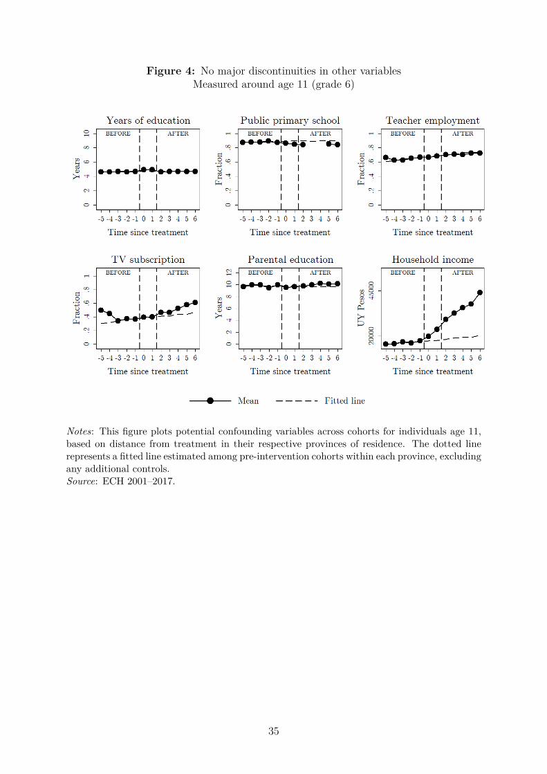
Figure 4: No major discontinuities in other variablesMeasured around age 11 (grade 6)

Notes: This figure plots potential confounding variables across cohorts for individuals age 11,based on distance from treatment in their respective provinces of residence. The dotted linerepresents a fitted line estimated among pre-intervention cohorts within each province, excludingany additional controls.Source: ECH 2001–2017.

35

Figure 5: Evolution of fraction enrolled in high school and post–secondary educationMeasured around age 19 across cohorts and provinces

Notes: This figure plots educational attainment by age 19 across cohorts based on time sincetreatment in their respective provinces. Panel A plots the average schooling in the population(years completed). The subsequent panels plot the fraction of individuals who enrolled in highschool (B), who graduated from high school (C) and who enrolled in postsecondary education(D). A cohort is defined as the group of individuals who are expected to start primary schoolin the same academic year, and is estimated based on age, year, and month of the survey.In-between cohorts were exposed to the program to the extent that some individuals startedprimary school later than expected or repeated grades by the time the program arrived in theirprovince.Source: ECH 2009–2017.

36

Table 1: Analysis of baseline characteristics

Complete sample Doughnut sampleMean Test SE Clustered SE Robust Test SE Clustered SE Robust

A. Around age 11 (5 years of education)Male 0.526 -0.00982 (0.0198) (0.0198) 0.532 (0.0190) (0.0267)Public school 0.864 -0.0405* (0.0225) (0.0225) 0.865 (0.0233) (0.0210)Lagging behind 0.355 0.0146 (0.0258) (0.0258) 0.344 (0.0258) (0.0255)Years of education 4.722 -0.0404 (0.0543) (0.0543) 4.669 (0.0538) (0.0619)Younger siblings 0.467 -0.00784 (0.0203) (0.0203) 0.460 (0.0224) (0.0267)Household size 4.997 -0.117 (0.0954) (0.0954) 4.987 (0.102) (0.104)Parent w/high school 0.767 -0.0386 (0.0350) (0.0228) 0.772 (0.0348) (0.0226)Parent w/college 0.175 0.00975 (0.0228) (0.0350) 0.175 (0.0225) (0.0199)Parental education (years) 9.870 -0.0527 (0.283) (0.283) 9.942 (0.274) (0.220)Household income ($ UY) 26,834 2,955 (2363.0) (2363.0) 3,276 (2,592) (1,663)TV subscription 0.457 0.0120 (0.0590) (0.0590) 0.471 (0.0581) (0.0255)Teacher employment 0.684 0.0140 (0.0159) (0.0159) 0.686 (0.0162) (0.00238)Teacher income (> p50) 0.622 0.0108 (0.0103) (0.00229) 0.0148 (0.0102) (0.00229)

N=16,271 N=11,409B. Before program, in 2006Computer at home 0.290 -0.0538*** (0.0120) (0.0117) -0.0557*** (0.0126) (0.0117)Internet connection 0.139 -0.0126 (0.0135) (0.00912) -0.0130 (0.0130) (0.00916)Mobile phone (not smart) 0.609 0.0120 (0.00873) (0.0117) 0.0127 (0.00919) (0.0118)Government aid 0.294 0.00317 (0.0102) (0.0111) 0.00218 (0.0111) (0.0111)Household income ($ UY) 20,809 66.73 (404.3) (576.7) 120.5 (416.8) (579.2)Nonwhite 0.157 -0.0119 (0.0116) (0.00881) -0.0141 (0.0119) (0.00884)

N=55,608 N=47,216Notes: The first column reports the average values for each variable. The other columns reportestimates of θ obtained from estimating equation 1 without control variables. Regressionsinclude nine cohorts in total, including three pre-intervention and two post-intervention cohortsin each province. This classification is based on current province of residence. Robust andprovince-clustered standard errors are reported.Source: ECH 2001-2017.* p < 0.1, ** p < 0.05, *** p < 0.01.

37

Table 2: Descriptive Statistics: individuals aged 18–20

Household Survey Data Administrative Data From[2011–2017] Public University System [2012–2016]

Variable Mean Variable Mean

Males 0.511 Age 19.35Nonwhite 0.171 Male 0.383Below poverty line 0.133 Born in Montevideo 0.55Household size 4.31 Public primary school 0.68Lives with parents 0.832 Public secondary school 0.631Has children 0.177 Children 0.002Employed 0.417 Lives with parents 0.725Has computer at home 0.806 Lives alone 0.044Has internet at home 0.628 Father post secondary education 0.234Has a non-Ceibal computer at home 0.628 Mother post secondary education 0.307Computers per person 0.488 First to attend post secondary 0.478Used computer last month 0.758 First to attend university 0.653Uses internet every day 0.64 Works 0.128Primary school was public 0.861 Scholarship 0.304Middle school was public 0.848 Technical major 0.178University was public 0.86 Multiple majors 0.141Ever enrolled in high school 0.588 Previous post-secondary studies 0.02Graduated from high school 0.285Ever enrolled in technical school 0.121Graduated from technical school 0.039Ever enrolled in post-secondary education 0.218Ever enrolled in university 0.179

Notes: Summary statistics (means) for individuals aged 18–20.Source: ECH 2011–2017 and Universidad de la Republica del Uruguay, 2012–2016.

38

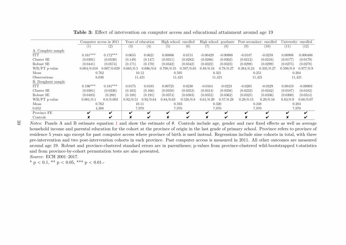
Table 3: Effect of intervention on computer access and educational attainment around age 19

Computer access in 2011 Years of education High school: enrolled High school: graduate Post-secondary: enrolled University: enrolled(1) (2) (3) (4) (5) (6) (7) (8) (9) (10) (11) (12)

A. Complete sampleITT 0.161*** 0.172*** 0.0655 0.0621 0.00806 0.0151 -0.00429 -0.00900 -0.0187 -0.0259 0.00908 0.000486Cluster SE (0.0391) (0.0530) (0.149) (0.147) (0.0311) (0.0282) (0.0286) (0.0302) (0.0212) (0.0216) (0.0177) (0.0179)Robust SE (0.0441) (0.0574) (0.171) (0.170) (0.0342) (0.0342) (0.0322) (0.0323) (0.0298) (0.0299) (0.0275) (0.0278)WB/PT p-value 0.004/0.018 0.007/0.029 0.665/0.5 0.696/0.6 0.798/0.55 0.597/0.65 0.88/0.34 0.78/0.27 0.384/0.24 0.335/0.27 0.599/0.8 0.977/0.9Mean 0.762 10.12 0.595 0.321 0.251 0.204Observations 6,038 11,421 11,421 11,421 11,421 11,421B. Doughnut sampleITT 0.196*** 0.181*** 0.0175 0.0185 0.00725 0.0230 -0.0164 -0.0223 -0.0265 -0.0329 0.00419 -0.00903Cluster SE (0.0381) (0.0336) (0.163) (0.166) (0.0358) (0.0353) (0.0314) (0.0338) (0.0233) (0.0242) (0.0187) (0.0182)Robust SE (0.0483) (0.288) (0.188) (0.191) (0.0374) (0.0383) (0.0352) (0.0362) (0.0325) (0.0336) (0.0300) (0.0314)WB/PT p-value 0.001/0.1 0.8/0.003 0.92/0.51 0.92/0.64 0.84/0.63 0.528/0.8 0.61/0.29 0.57/0.28 0.29/0.15 0.29/0.16 0.83/0.9 0.68/0.07Mean 0.762 10.11 0.593 0.320 0.248 0.2040.652 4,308 7,970 7,970 7,970 7,970 7,970Province FE 4 4 4 4 4 4 4 4 4 4 4 4

Controls 8 4 8 4 8 4 8 4 8 4 8 4

Notes: Panels A and B estimate equation 1 and show the estimate of θ. Controls include age, gender and race fixed effects as well as averagehousehold income and parental education for the cohort at the province of origin in the last grade of primary school. Province refers to province ofresidence 5 years ago except for past computer access where province of birth is used instead. Regressions include nine cohorts in total, with threepre-intervention and two post-intervention cohorts in each province. Past computer access is measured in 2011. All other outcomes are measuredaround age 19. Robust and province-clustered standard errors are in parentheses; p-values from province-clustered wild-bootstrapped t-statisticsand from province-by-cohort permutation tests are also presented.Source: ECH 2001–2017.* p < 0.1, ** p < 0.05, *** p < 0.01.-

39

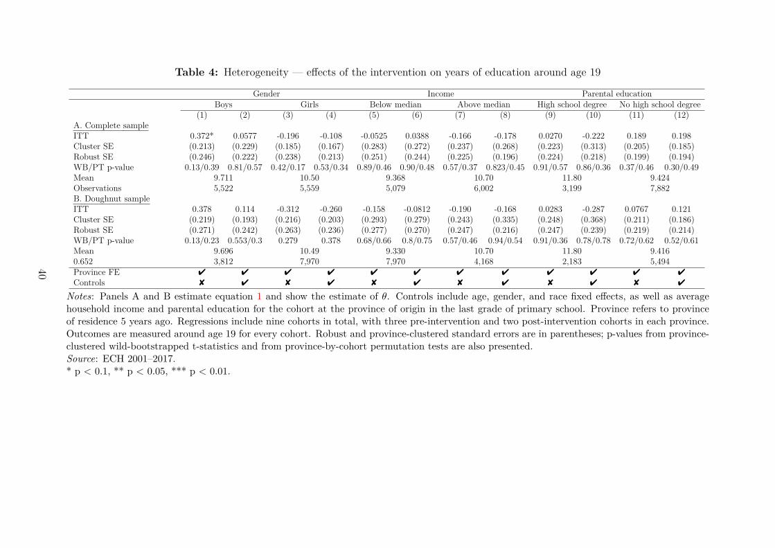
Table 4: Heterogeneity — effects of the intervention on years of education around age 19

Gender Income Parental educationBoys Girls Below median Above median High school degree No high school degree

(1) (2) (3) (4) (5) (6) (7) (8) (9) (10) (11) (12)A. Complete sampleITT 0.372* 0.0577 -0.196 -0.108 -0.0525 0.0388 -0.166 -0.178 0.0270 -0.222 0.189 0.198Cluster SE (0.213) (0.229) (0.185) (0.167) (0.283) (0.272) (0.237) (0.268) (0.223) (0.313) (0.205) (0.185)Robust SE (0.246) (0.222) (0.238) (0.213) (0.251) (0.244) (0.225) (0.196) (0.224) (0.218) (0.199) (0.194)WB/PT p-value 0.13/0.39 0.81/0.57 0.42/0.17 0.53/0.34 0.89/0.46 0.90/0.48 0.57/0.37 0.823/0.45 0.91/0.57 0.86/0.36 0.37/0.46 0.30/0.49Mean 9.711 10.50 9.368 10.70 11.80 9.424Observations 5,522 5,559 5,079 6,002 3,199 7,882B. Doughnut sampleITT 0.378 0.114 -0.312 -0.260 -0.158 -0.0812 -0.190 -0.168 0.0283 -0.287 0.0767 0.121Cluster SE (0.219) (0.193) (0.216) (0.203) (0.293) (0.279) (0.243) (0.335) (0.248) (0.368) (0.211) (0.186)Robust SE (0.271) (0.242) (0.263) (0.236) (0.277) (0.270) (0.247) (0.216) (0.247) (0.239) (0.219) (0.214)WB/PT p-value 0.13/0.23 0.553/0.3 0.279 0.378 0.68/0.66 0.8/0.75 0.57/0.46 0.94/0.54 0.91/0.36 0.78/0.78 0.72/0.62 0.52/0.61Mean 9.696 10.49 9.330 10.70 11.80 9.4160.652 3,812 7,970 7,970 4,168 2,183 5,494Province FE 4 4 4 4 4 4 4 4 4 4 4 4

Controls 8 4 8 4 8 4 8 4 8 4 8 4

Notes: Panels A and B estimate equation 1 and show the estimate of θ. Controls include age, gender, and race fixed effects, as well as averagehousehold income and parental education for the cohort at the province of origin in the last grade of primary school. Province refers to provinceof residence 5 years ago. Regressions include nine cohorts in total, with three pre-intervention and two post-intervention cohorts in each province.Outcomes are measured around age 19 for every cohort. Robust and province-clustered standard errors are in parentheses; p-values from province-clustered wild-bootstrapped t-statistics and from province-by-cohort permutation tests are also presented.Source: ECH 2001–2017.* p < 0.1, ** p < 0.05, *** p < 0.01.

40

Table 5: Understanding the findings — effects of the intervention on early parenthood, employment, and technology use by age 19

Teen Parent Employed Current computer access Computer & internet use Internet for information & education(1) (2) (3) (4) (5) (6) (7) (8) (9) (10)

A. Complete sampleITT -0.0704*** -0.0628*** -0.0306 -0.0356 -0.0702*** -0.0706*** 0.0411 0.0234 0.0403* 0.0280Cluster SE (0.0140) (0.0169) (0.0261) (0.0302) (0.0213) (0.0224) (0.0384) (0.0357) (0.0227) (0.0257)Robust SE (0.0226) (0.0222) (0.0345) (0.0339) (0.0275) (0.0279) (0.0337) (0.0338) (0.0304) (0.0305)WB/PT p-value 0.008/0.43 0.018/0.42 0.24/0.36 0.26/0.35 0.026/0.04 0.032/0.04 0.327/0.92 0.565/0.93 0.178/0.54 0.334/0.57Mean 0.110 0.446 0.800 0.576 0.739Observations 11,421 11,421 11,421 11,421 11,421B. Doughnut sampleITT -0.0683*** -0.0612*** -0.0502 -0.0545 -0.0953*** -0.0896*** 0.0559 0.0532 0.0151 0.00473Cluster SE (0.0114) (0.0145) (0.0291) (0.0347) (0.0210) (0.0240) (0.0396) (0.0380) (0.0250) (0.0296)Robust SE (0.0247) (0.0248) (0.0377) (0.0381) (0.0302) (0.0317) (0.0370) (0.0381) (0.0335) (0.0344)WB/PT p-value 0.002/0.75 0.005/0.72 0.07/0.497 0.152/0.64 0.002/0.16 0.002/0.17 0.160/0.58 0.201/0.71 0.546/0.69 0.875/0.74Mean 0.110 0.444 0.794 0.554 0.7360.652 4,308 7,970 7,970 7,970 7,970Province FE 4 4 4 4 4 4 4 4 4 4

Controls 8 4 8 4 8 4 8 4 8 4

Notes: Panels A and B estimate equation 1 and show the estimate of θ. Controls include age, gender, and race fixed effects, as well as averagehousehold income and parental education for the cohort at the province of origin in the last grade of primary school, where province of originrefers to province of residence five years ago. Regressions include nine cohorts in total, with three pre-intervention and two post-interventioncohorts in each province. Outcomes are measured around age 19. Robust and province-clustered standard errors are in parentheses; p-values fromprovince-clustered wild-bootstrapped t-statistics and from province-by-cohort permutation tests are also presented.Source: ECH 2001–2017.* p < 0.1, ** p < 0.05, *** p < 0.01.

41

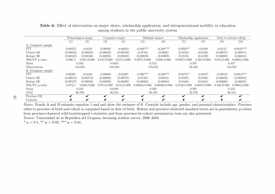
Table 6: Effect of intervention on major choice, scholarship application, and intergenerational mobility in educationamong students in the public university system

Technological major Computer major Multiple majors Scholarship application First to attend college(1) (2) (3) (4) (5) (6) (7) (8) (9) (10)

A. Complete sampleITT 0.00373 -0.0120 -0.00850 -0.00943 -0.286*** -0.288*** -0.0320** -0.0188 -0.0113 0.0844***Cluster SE (0.00832) (0.00848) (0.00650) (0.00559) (0.0716) (0.0622) (0.0134) (0.0126) (0.00675) (0.00811)Robust SE (0.00522) (0.00536) (0.00288) (0.00292) (0.00859) (0.00890) (0.0135) (0.0129) (0.00692) (0.00612)WB/PT p-value 0.696/1 0.691/0.000 0.847/0.000 0.671/0.000 0.0071/0.000 0.006/0.000 0.0897/0.000 0.301/0.000 0.052/0.000 0.0004/0.000Mean 0.163 0.0424 0.313 0.301 0.447Observations 110,023 110,032 110,032 56,324 110,032B. Doughnut sampleITT 0.00397 -0.0109 -0.00869 -0.0109* -0.300*** -0.290*** -0.0472** -0.0316* -0.00512 0.0914***Cluster SE (0.00819) (0.00773) (0.00669) (0.00578) (0.0749) (0.0618) (0.0187) (0.0166) (0.00683) (0.00859)Robust SE (0.00527) (0.00550) (0.00290) (0.00299) (0.00862) (0.00884) (0.0166) (0.0164) (0.00698) (0.00625)WB/PT p-value 0.674/1 0.669/0.000 0.873/0.000 0.612/0.000 0.00680/0.000 0.00600/0.000 0.0128/0.000 0.0897/0.000 0.426/0.000 0.0004/0.000Mean 0.164 0.0430 0.288 0.301 0.4450.652 86,190 86,194 86,194 32,726 86,194Province FE 4 4 4 4 4 4 4 4 4 4

Controls 8 4 8 4 8 4 8 4 8 4

Notes: Panels A and B estimate equation 1 and and show the estimate of θ. Controls include age, gender, and parental characteristics. Provincerefers to province of birth and cohort is computed based on date of birth. Robust and province-clustered standard errors are in parentheses; p-valuesfrom province-clustered wild-bootstrapped t-statistics and from province-by-cohort permutation tests are also presented.Source: Universidad de la Republica del Uruguay, incoming student survey, 2006–2016.* p < 0.1, ** p < 0.05, *** p < 0.01.

42

Table 7: Effect of intervention on area of study at university

Arts Agrarian Sciences Social Sciences Science and Technology Health(1) (2) (3) (4) (5) (6) (7) (8) (9) (10)

A. Complete sampleITT -0.007*** -0.005*** -0.018** -0.019** -0.025* -0.021 0.020 0.005 0.030*** 0.041***Cluster SE (0.001) (0.001) (0.007) (0.008) (0.015) (0.015) (0.015) (0.015) (0.006) (0.007)Robust SE (0.002) (0.002) (0.003) (0.003) (0.007) (0.007) (0.006) (0.006) (0.006) (0.006)Mean 0.017 0.063 0.437 0.227 0.255Observations 109,978B. Doughnut sampleITT -0.006*** -0.005*** -0.018** -0.019** -0.027* -0.022 0.020 0.005 0.031*** 0.041***Cluster SE (0.001) (0.001) (0.008) (0.008) (0.015) (0.016) (0.015) (0.015) (0.007) (0.007)Robust SE (0.002) (0.002) (0.003) (0.003) (0.007) (0.007) (0.006) (0.006) (0.006) (0.006)Mean 0.017 0.064 0.439 0.228 0.251Observations 86,146Province FE 4 4 4 4 4 4 4 4 4 4

Controls 8 4 8 4 8 4 8 4 8 4

Notes: This table reports the marginal effects resulting from estimating equation 1 using a multinomial logit model. The largest category, socialsciences, is used as the baseline Province refers to province of birth and cohort is computed based on date of birth. Controls include age, gender,and parental characteristics. Robust and province-clustered standard errors are in parenthesis.Source: Universidad de la Republica del Uruguay, incoming student survey, 2006–2016.* p < 0.1, ** p < 0.05, *** p < 0.01.

43