Techniques de Reformulation en Programmation Mathématique

UNIVERSITE PARIS IXLAMSADE

Memoire presente en vue de l’obtention de l’Habilitationa Diriger des Recherches

Techniques de Reformulation en ProgrammationMathematique

Leo LibertiLIX, Ecole Polytechnique, Palaiseau, 91128 France

[email protected]

November 16, 2007

Jury:

Philippe MICHELON (Rapporteur), Professeura l’Universite d’Avignon

Nelson MACULAN (Rapporteur), Professeura l’Universidade Federal do Rio de Janeiro (Brazil)

Hanif SHERALI (Rapporteur), Professeur au Virginia Polytechnic Institute (USA)

Alain BILLIONNET (Examinateur), Professeur au Conservatoir Nationald’Arts et Metiers

Abdel LISSER (Examinateur), Professeura l’Universite de Paris XI (Sud)

Philippe BAPTISTE (Examinateur), Professeura l’Ecole Polytechnique

Tapio WESTERLUND (Examinateur), Professeura l’Universite de Abø (Finlande)

Vangelis PASCHOS (Coordinateur), Professeura l’Universite Paris IX (Dauphine)

Resume

L’objet centrale de cette these est l’utilisation de techniques de reformulations en program-

mation mathematique. Les problemes d’optimisation et de decision peuventetre decrits preci-

sement par une formulation composee de: parametres numeriques, variables de decision (leur

valeursetant determinees grace au resultat d’un proces algorithmique), une ou plusieurs fonc-

tions objectivesa optimiser, et plusieurs ensembles de contraintes; fonctions objectives et con-

traintes peuventetre exprimees explicitement comme functions de parametres et variables, ou

implicitement comme conditions sur les variables. Ceselements, c’esta dire parametres, vari-

ables, fonctions objectives et contraintes, forment un langage appele programmation mathema-

tique. Pour chaque probleme donne d’optimisation ou decision, il y a d’habitude un nombre

infini de differents formulations de programmation mathematique possibles. Selon l’algorithme

utilise pour les resoudre, formulations distinctes sont plus ou moins efficaces et/ou efficientes.

En outre, plusieurs sous-problemes ressortants de l’algorithme de solution peuvent eux-memes

etre formules comme des problemes de programmation mathematique (appeles problemes aux-

iliaires). Cette these presente unetude approfondi des transformations symboliques qui map-

pent des formulations de programmation mathematique a leur formesequivalentes et autres

formulations relies, et de leur impacte sur les algorithmes de solution.

Abstract

This thesis concerns the use of reformulation techniques inmathematical programming. Op-

timization and decision problems can be cast into a formulation involving sets of known numer-

ical parameters, decision variables whose value is to be determined as a result of an algorithmic

process, one of more optional objective functions to be optimized and various sets of constraints,

which can be either expressed explicitly as functions of theparameters and variables, or as im-

plicit requirements on the variables. These elements, namely parameters, variables, objective(s)

and constraints, form a language called mathematical programming. There are usually many

different possible equivalent mathematical programming formulations for the same optimiza-

tion or decision problem. Different formulations often perform differently according to the type

of algorithm employed to solve the problem. Furthermore, related auxiliary problems which

may be useful during the course of the algorithmic solution process may arise and be also cast

as mathematical programming formulations. This thesis is an in-depth study of the symbolic

transformations that map a mathematical programming formulation to its equivalent forms and

to other useful related formulations, and of their relations to various solution algorithms.

Contents

1 Introduction 8

2 General framework 14

2.1 A data structure for mathematical programming formulations . . . . . . . . . . 14

2.1.1 Examples . . . . . . . . . . . . . . . . . . . . . . . . . . . . . . . . . 16

2.1.1.1 A quadratic problem . . . . . . . . . . . . . . . . . . . . . . 16

2.1.1.2 Balanced graph bisection . . . . . . . . . . . . . . . . . . . 16

2.1.1.3 The Kissing Number Problem . . . . . . . . . . . . . . . . . 18

2.2 A data structure for mathematical expressions . . . . . . . .. . . . . . . . . . 20

2.2.1 Standard form . . . . . . . . . . . . . . . . . . . . . . . . . . . . . . . 21

2.3 Theoretical results . . . . . . . . . . . . . . . . . . . . . . . . . . . . . .. . . 22

2.4 Standard forms in mathematical programming . . . . . . . . . .. . . . . . . . 29

2.4.1 Linear Programming . . . . . . . . . . . . . . . . . . . . . . . . . . . 30

2.4.2 Mixed Integer Linear Programming . . . . . . . . . . . . . . . . .. . 30

2.4.3 Nonlinear Programming . . . . . . . . . . . . . . . . . . . . . . . . . 30

2.4.4 Mixed Integer Nonlinear Programming . . . . . . . . . . . . . .. . . 31

2.4.5 Separable problems . . . . . . . . . . . . . . . . . . . . . . . . . . . . 31

2.4.6 Factorable problems . . . . . . . . . . . . . . . . . . . . . . . . . . . 32

2.4.7 D.C. problems . . . . . . . . . . . . . . . . . . . . . . . . . . . . . . 32

Contents 4

2.4.8 Linear Complementarity problems . . . . . . . . . . . . . . . . . .. . 33

2.4.9 Bilevel Programming problems . . . . . . . . . . . . . . . . . . . . .34

2.4.10 Semidefinite Programming problems . . . . . . . . . . . . . . .. . . 34

3 Reformulations 36

3.1 Elementary reformulations . . . . . . . . . . . . . . . . . . . . . . . .. . . . 36

3.1.1 Objective function direction . . . . . . . . . . . . . . . . . . . .. . . 36

3.1.2 Constraint sense . . . . . . . . . . . . . . . . . . . . . . . . . . . . . 37

3.1.3 Liftings, restrictions and projections . . . . . . . . . . .. . . . . . . . 37

3.1.3.1 Lifting . . . . . . . . . . . . . . . . . . . . . . . . . . . . . 37

3.1.3.2 Restriction . . . . . . . . . . . . . . . . . . . . . . . . . . . 37

3.1.3.3 Projection . . . . . . . . . . . . . . . . . . . . . . . . . . . 38

3.1.4 Equations to inequalities . . . . . . . . . . . . . . . . . . . . . . .. . 38

3.1.5 Inequalities to equations . . . . . . . . . . . . . . . . . . . . . . .. . 39

3.1.6 Absolute value terms . . . . . . . . . . . . . . . . . . . . . . . . . . . 40

3.1.7 Product of exponential terms . . . . . . . . . . . . . . . . . . . . .. . 40

3.1.8 Binary to continuous variables . . . . . . . . . . . . . . . . . . . .. . 40

3.1.9 Integer to binary variables . . . . . . . . . . . . . . . . . . . . . .. . 41

3.1.9.1 Assignment variables . . . . . . . . . . . . . . . . . . . . . 41

3.1.9.2 Binary representation . . . . . . . . . . . . . . . . . . . . . 42

3.1.10 Feasibility to optimization problems . . . . . . . . . . . .. . . . . . . 42

3.2 Exact linearizations . . . . . . . . . . . . . . . . . . . . . . . . . . . . .. . . 44

3.2.1 Piecewise linear objective functions . . . . . . . . . . . . .. . . . . . 44

3.2.2 Product of binary variables . . . . . . . . . . . . . . . . . . . . . .. . 44

3.2.3 Product of binary and continuous variables . . . . . . . . .. . . . . . 45

Contents 5

3.2.4 Complementarity constraints . . . . . . . . . . . . . . . . . . . . .. . 45

3.2.5 Minimization of absolute values . . . . . . . . . . . . . . . . . .. . . 46

3.2.6 Linear fractional terms . . . . . . . . . . . . . . . . . . . . . . . . .. 47

3.3 Advanced reformulations . . . . . . . . . . . . . . . . . . . . . . . . . .. . . 47

3.3.1 Hansen’s Fixing Criterion . . . . . . . . . . . . . . . . . . . . . . . .48

3.3.2 Compact linearization of binary quadratic problems . .. . . . . . . . . 48

3.3.3 Reduction Constraints . . . . . . . . . . . . . . . . . . . . . . . . . . 49

3.4 Advanced examples . . . . . . . . . . . . . . . . . . . . . . . . . . . . . . . .50

3.4.1 The Hyperplane Clustering Problem . . . . . . . . . . . . . . . . .. . 50

3.4.2 Selection of software components . . . . . . . . . . . . . . . . .. . . 53

4 Relaxations 58

4.1 Definitions . . . . . . . . . . . . . . . . . . . . . . . . . . . . . . . . . . . . . 59

4.2 Elementary relaxations . . . . . . . . . . . . . . . . . . . . . . . . . . .. . . 59

4.2.1 Outer approximation . . . . . . . . . . . . . . . . . . . . . . . . . . . 60

4.2.2 αBB convex relaxation . . . . . . . . . . . . . . . . . . . . . . . . . . 61

4.2.3 Branch-and-Contract convex relaxation . . . . . . . . . . . . .. . . . 62

4.2.4 Symbolic reformulation based convex relaxation . . . .. . . . . . . . 62

4.2.5 BARON’s convex relaxation . . . . . . . . . . . . . . . . . . . . . . .63

4.3 Advanced relaxations . . . . . . . . . . . . . . . . . . . . . . . . . . . . .. . 63

4.3.1 Lagrangian relaxation . . . . . . . . . . . . . . . . . . . . . . . . . .64

4.3.2 Semidefinite relaxation . . . . . . . . . . . . . . . . . . . . . . . . .. 65

4.3.3 Reformulation-Linearization Technique . . . . . . . . . . .. . . . . . 66

4.3.3.1 Basic RLT . . . . . . . . . . . . . . . . . . . . . . . . . . . 66

4.3.3.2 RLT Hierarchy . . . . . . . . . . . . . . . . . . . . . . . . . 68

Contents 6

4.3.4 Signomial programming relaxations . . . . . . . . . . . . . . .. . . . 69

4.4 Valid cuts . . . . . . . . . . . . . . . . . . . . . . . . . . . . . . . . . . . . . 70

4.4.1 Valid cuts for MILPs . . . . . . . . . . . . . . . . . . . . . . . . . . . 71

4.4.2 Valid cuts for NLPs . . . . . . . . . . . . . . . . . . . . . . . . . . . . 72

4.4.3 Valid cuts for MINLPs . . . . . . . . . . . . . . . . . . . . . . . . . . 74

5 Conclusion 75

Bibliography 76

List of Figures

2.1 The graphse1 (above) ande2 (below) from Example 2.1.1.1. . . . . . . . . . . 17

2.2 The BGBP instance in Example 2.1.1.1. . . . . . . . . . . . . . . . . . .. . . 18

2.3 The graphe′1 from Example 2.1.1.2.L′ij = Lij + Lji for all i, j. . . . . . . . . 19

2.4 The Kissing Number Problem in 3D. A configuration with 12 balls found by a

Variable Neighbourhood Search global optimization solver. . . . . . . . . . . . 20

2.5 Plots ofsin(x) and 12x+ sin(x). . . . . . . . . . . . . . . . . . . . . . . . . . 25

4.1 Piecewise linear underestimating approximations for concave (left) and convex

(right) univariate functions. . . . . . . . . . . . . . . . . . . . . . . . .. . . . 70

4.2 A γ-valid cut. . . . . . . . . . . . . . . . . . . . . . . . . . . . . . . . . . . . 73

Chapter 1

Introduction

Optimization and decision problems are usually defined by their input and a mathematical

description of the required output: a mathematical entity with an associated value, or whether

a given entity has a specified mathematical property or not. These mathematical entities and

properties are expressed in the language of set theory, mostoften in the ZFC axiomatic system

[55] (for clarity, a natural language such as English is usually employed in practice). The scope

of set theory language in ZFC is to describe all possible mathematical entities, and its limits are

given by Godel’s incompleteness theorem.

Optimization and decision problems are special in the sensethat they are closely linked to a

particular algorithmic process designed to solve them: more precisely, although the algorithm is

not directly mentioned in the problem definition, the main reason why problems are cast is that

a solution to the problem is desired. In this respect the usual set theoretical language, with all

its expressive powers, falls short of this requirement: specifically, no algorithm is so “generic”

that it can solve all problems formulated in terms of set theory. Just to make an example, all

Linear Programming (LP) problems can be expressed in a language involving real numbers,

variables, a linear form to be minimized, a system of linear equations to be satisfied, and a set

of non-negativity constraints on the variables. This particular language used for describing LPs

has much stricter limits than the set-theoretical languageused in ZFC, of course. On the other

hand there exists an algorithm, namely the simplex algorithm [24], which is generic enough to

solve any LP problem, and which performs well in practice.

In its most general terms, a decision problem can be expressed as follows: given a setW

and a subsetD ⊆ W , decide whether a givenx ∈ W belongs toD or not. Even supposing

thatW has finite cardinality (so that the problem is certainly decidable), the only algorithm

which is generic enough to solve this problem is complete enumeration, whose low efficiency

Chapter 1. Introduction 9

renders it practically useless. Informally speaking, whendiscussing decidable problems and

solution algorithms, there is a trade-off between how powerful is the language used to express

the problems, and how efficient the associated solution algorithm is.

Mathematical programming can be seen as a language which is powerful enough to ex-

press almost all practically interesting optimization anddecision problems. Mathematical pro-

gramming formulations can be categorized according to various properties, and rather efficient

solution algorithms exist for many of the categories. The semantic scope of mathematical pro-

gramming is to define optimization and decision problems: asthis scope is narrower than that

of the set theoretical language of ZFC, according to the trade-off principle mentioned above,

the associated generic algorithms are more efficient.

As in most languages, the same concept can be expressed in many ways. More precisely,

there are many equivalent formulations for each given problem (what the term “equivalent”

means in this context will be defined later). Furthermore, solution algorithms for mathematical

programming formulations often rely on solving a sequence of different problems (often termed

auxiliary problems) related to the original one: although these are usually notequivalent to the

original problem, they may be relaxations, projections, liftings, decompositions (among oth-

ers). The relations between the original and auxiliary problems are expressed in the literature

by means of logical, algebraic and/or transcendental expressions which draw on the same fa-

miliar ZFC language. As long as theoretical statements are being made, there is nothing wrong

with this, for people are usually able to understand that language. There is, however, a big gap

between understanding the logical/algebraic relations among sets of optimization problems, and

being able to implement algorithms using these problems in various algorithmic steps. Existing

data structures and code libraries usually offer numericalrather than symbolic facilities. Sym-

bolic algorithms and libraries exist, but they are not purpose-built to deal with optimization and

decision problems.

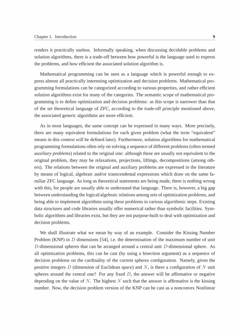
We shall illustrate what we mean by way of an example. Considerthe Kissing Number

Problem (KNP) inD dimensions [54], i.e. the determination of the maximum number of unit

D-dimensional spheres that can be arranged around a central unit D-dimensional sphere. As

all optimization problems, this can be cast (by using a bisection argument) as a sequence of

decision problems on the cardinality of the current spheresconfiguration. Namely, given the

positive integersD (dimension of Euclidean space) andN , is there a configuration ofN unit

spheres around the central one? For any fixedD, the answer will be affirmative or negative

depending on the value ofN . The highestN such that the answer is affirmative is the kissing

number. Now, the decision problem version of the KNP can be cast as a nonconvex Nonlinear


Programming (NLP) feasibility problem as follows. For alli ≤ N , let xi = (xi1, . . . , xiD) ∈

RD be the center of thei-th sphere. We look for a set of vectorsxi | i ≤ N satisfying the

following constraints:

∀ i ≤ N ||xi|| = 2

∀ i < j ≤ N ||xi − xj|| ≥ 2

∀ i ≤ N − 2 ≤ xi ≤ 2.

It turns out that this problem is numerically quite difficultto solve, as it is very unlikely that the

local NLP solution algorithm will be able to compute a valid feasible starting solution straight

away. Failing to find an initial feasible solution means thatthe solver will immediately abort

without having made any progress. Most researchers with some experience in NLP solvers

(such as e.g. SNOPT [36]), however, will immediately reformulate this problem into a more

computationally amenable form by squaring the norms to get rid of a potentially problematic

square root, and treating the reverse convex constraints||xi − xj|| ≥ 2 as soft constraints by

multiplying the right hand sides by a non-negative scaling variableα, which is then maximized:

maxα (1.1)

∀ i ≤ N ||xi||2 = 4 (1.2)

∀ i < j ≤ N ||xi − xj||2 ≥ 4α. (1.3)

∀ i ≤ N − 2 ≤ xi ≤ 2 (1.4)

α ≥ 0. (1.5)

In this form, finding an initial feasible solution is trivial; for example,xi = (2, 0, . . . , 0) for all

i ≤ N will do. Subsequent solver iteration will likely be able to provide a solution. Should

the computed value ofα be≥ 1, the solution would be feasible in the hard constraints, too.

Currently, we are aware of no optimization language environment that is able to perform the

described reformulation automatically. Whilst this is not ahuge limitation for NLP experts,

people who simply wish to model a problem and get its solutionwill fail to obtain one, and may

even be led into thinking that the formulation itself is infeasible.

Another insightful example of the types of limitations we refer to can be drawn from the

KNP. We might wish to impose ordering constraints on some of the spheres to reduce the num-

ber of symmetric solutions. Ordering spheres packed on a spherical surface is hard to do in Eu-

clidean coordinates, but it can be done rather easily in spherical coordinates, by simply stating

that the value of a spherical coordinate of thei-th sphere must be smaller than the corresponding

value in thej-th sphere. We can transform a Euclidean coordinate vectorx = (x1, . . . , xD) in


D-spherical coordinates(ρ, ϑ1, . . . , ϑD−1) such thatρ = ||x|| andϑ ∈ [0, 2π]D−1 by means of

the following equations:

ρ = ||x|| (1.6)

∀k ≤ D xk = ρ sinϑk−1

D−1∏

h=k

cosϑh (1.7)

(this yields another NLP formulation of the KNP). Applying theD-spherical transformation is

simply a matter of symbolic term replacement and algebraic simplification, and yet no opti-

mization language environment offers such capabilities. Bycarrying things further, we might

wish to devise an algorithm that dynamically inserts or removes constraints expressed in either

Euclidean or spherical coordinates depending on the statusof the current solution, and re-solves

the (automatically) reformulated problem at each iteration. This may currently be done (up to a

point) by optimization language environments such as AMPL [34], provided all constraints are

part of a pre-specified family of parametric constraints. Creating new constraints by symbolic

term replacement, however, is not a task that can currently be carried out automatically.

The limitations emphasized in the KNP example illustrate a practical need for very sophisti-

cated software including numerical as well as symbolic algorithms, both applied to the unique

goal of solving optimization problems cast as mathematicalprogramming formulations. The

current state of affairs is that there are many numerical optimization solvers and many Com-

puter Algebra Systems (CAS) — such as Maple or Mathematica — whose efficiency is severely

hampered by the full generality of their capabilities. In short, we would ideally need (small)

parts of the symbolic kernels driving the existing CASes to becombined with the existing opti-

mization algorithms, plus a number of super-algorithms capable of making automated, dynamic

decisions on the type of reformulations that are needed to improve the current search process.

Although the above paradigm might seem far-fetched, it doesin fact already exist in the form

of the hugely successful CPLEX [47] solver targeted at solving Mixed-Integer Linear Program-

ming (MINLP) problems. The initial formulation provided bythe user is automatically simpli-

fied and improved with a considerable number of pre-processing steps which attempt to reduce

the number of variables and constraints. Thereafter, at each node of the Branch-and-Bound

algorithm, the formulation may be tightened as needed by inserting and removing additional

valid constraints, in the hope that the current relaxed solution of the (automatically obtained)

linear relaxation is improved. Advanced users may of coursedecide to tune many parameters

controlling this process, but practitioners who simply need a practical answer can simply use

default parameters and to let CPLEX decide what is best. Naturally, the task carried out by

CPLEX is greatly simplified by the assumption that both objective function and constraints are


linear forms, which is obviously not the case in a general nonlinear setting.

In this thesis we attempt to move some steps in the direction of endowing general mathe-

matical programming with the same degree of algorithmic automation enjoyed by linear pro-

gramming. We propose: (a) a theoretical framework in which mathematical programming re-

formulations can be formalized in a unified way, and (b) a literature review of the most suc-

cessful existing reformulation and relaxation techniquesin mathematical programming. Since

an all-comprehensive literature review in reformulation techniques would extend this thesis to

possibly several hundreds (thousands?) pages, only a partial review has been provided. In this

sense, this should be seen as “work in progress” towards laying the foundations to a computer

software which is capable of reformulating mathematical programming formulations automat-

ically. Note also that for this reason, the usual mathematical notations have been translated to

a data structure framework that is designed to facilitate computer implementation. Most im-

portantly, “functions” — which as mathematical entities are interpreted as maps between sets

— are represented by expression trees: what is meant by the expressionx + y, for example,

is really a directed binary tree on the vertices+, x, y with arcs(+, x), (+, y). For clarity

purposes, however, we also provide the usual mathematical languages.

One last (but not least) remark is that reformulations can beseen as a new way of expressing

a known problem. Reformulations are syntactical operationsthat may add or remove variables

or constraints, whilst keeping the fundamental structure of the problem optima invariant. When

some new variables are added and some of the old ones are removed, we can usually try to

re-interpret the reformulated problem and assign a meaningto the new variables, thus gaining

new insights to the problem. One example of this is given in Sect. 3.4.2. One other area in

mathematical programming that provides a similarly clear relationship between mathematical

syntax and semantics is LP duality with the interpretation of reduced costs. This is important

insofar as it offers alternative interpretations to known problems, which gains new and useful

insights.

The rest of this thesis is organized as follows. In Chapter 2 wepropose a general theoret-

ical framework of definitions allowing a unified formalization of mathematical programming

reformulations. The definitions allow a consistent treatment of the most common variable and

constraint manipulations in mathematical programming formulations. In Chapter 3 we present

a systematic study of a set of well known reformulations. Most reformulations are listed as

symbolic algorithms acting on the problem structure, although the equivalent transformation in

mathematical terms is given for clarity purposes. In Chapter4 we present a systematic study

of a set of well known relaxations. Again, relaxations are listed as symbolic algorithms acting


on the problem structure whenever possible, the equivalentmathematical transformation being

given for clarity.

Chapter 2

General framework

In Sect. 2.1 we formally define what a mathematical programming formulation is. In Sect. 2.2

we discuss the expression tree function representation. InSect. 2.3 we discuss some types

of reformulations and establish some links between them. Sect. 2.4 lists the most common

standard forms in mathematical programming.

2.1 A data structure for mathematical programming formu-lations

In this Chapter we give a formal definition of a mathematical programming formulation in such

terms that can be easily implemented on a computer. We then give several examples to illustrate

the generality of our definition. We refer to a mathematical programming problem in the most

general form:min f(x)

g(x) ⋚ b

x ∈ X,

(2.1)

wheref, g are function sequences of various sizes,b is an appropriately-sized real vector, and

X is a cartesian product of continuous and discrete intervals.

The precise definition of a mathematical programming formulation lists the different formu-

lation elements: parameters, variables having types and bounds, expressions depending on the

parameters and variables, objective functions and constraints depending on the expressions. We

let P be the set of all mathematical programming formulations, and M be the set of all matri-

ces. This is used in Defn. 2.1.1 to define leaf nodes in mathematical expression trees, so that

Chapter 2. General framework 15

the concept of a formulation can also accommodate multilevel and semidefinite programming

problems.

2.1.1 DefinitionGiven an alphabetL consisting of countably manyalphanumeric namesNL and operator sym-bolsOL, amathematical programming formulationP is a 7-tuple(P ,V , E ,O, C,B, T ), where:

• P ⊆ NL is the sequence ofparameter symbols: each elementp ∈ P is aparameter name;

• V ⊆ NL is the sequence ofvariable symbols: each elementv ∈ V is avariable name;

• E is the set ofexpressions: each elemente ∈ E is a Directed Acyclic Graph (DAG)e = (Ve, Ae) such that:

(a) Ve ⊆ L is a finite set

(b) there is a unique vertexre ∈ Ve such thatδ−(re) = ∅ (such a vertex is called theroot vertex)

(c) verticesv ∈ Ve such thatδ+(v) = ∅ are calledleaf verticesand their set is denotedby λ(e); all leaf verticesv are such thatv ∈ P ∪ V ∪ R ∪ P ∪M

(d) for all v ∈ Ve such thatδ+(v) 6= ∅, v ∈ OL

(e) two weightingsχ, ξ : Ve → R are defined onVe: χ(v) is thenode coefficientandξ(v) is thenode exponentof the nodev; for any vertexv ∈ Ve, we letτ(v) be thesymbolic termof v: namely,v = χ(v)τ(v)ξ(v).

elements ofE are sometimes calledexpression trees; nodesv ∈ OL represent an operationon the nodes inδ+(v), denoted byv(δ+(v)), with output inR;

• O ⊆ −1, 1 × E is the sequence ofobjective functions; each objective functiono ∈ Ohas the form(do, fo) wheredo ∈ −1, 1 is theoptimization direction(−1 stands forminimization,+1 for maximization) andfo ∈ E;

• C ⊆ E × S × R (whereS = −1, 0, 1) is the sequence ofconstraintsc of the form(ec, sc, bc) with ec ∈ E, sc ∈ S, bc ∈ R:

c ≡

ec ≤ bc if sc = −1ec = bc if sc = 0ec ≥ bc if sc = 1;

• B ⊆ R|V| × R|V| is the sequence ofvariable bounds: for all v ∈ V let B(v) = [Lv, Uv]with Lv, Uv ∈ R;

• T ⊆ 0, 1, 2|V| is the sequence ofvariable types: for all v ∈ V, v is called acontinuousvariable if T (v) = 0, aninteger variableif T (v) = 1 and abinary variableif T (v) = 2.


We remark that for a sequence of variablesz ⊆ V we write T (z) and respectivelyB(z) to

mean the corresponding sequences of types and respectivelybound intervals of the variables

in z. Given a formulationP = (P ,V , E ,O, C,B, T ), thecardinality of P is |P | = |V|. We

sometimes refer to a formulation by calling it anoptimization problemor simply aproblem.

2.1.2 DefinitionAny formulationQ that can be obtained byP by a finite sequence of symbolic operationscarried out on the data structure is called aproblem transformation.

2.1.1 Examples

In this section we provide some explicitly worked out examples that illustrate Defn. 2.1.1.

2.1.1.1 A quadratic problem

Consider the problem of minimizing the quadratic form3x21 + 2x2

2 + 2x23 + 3x2

4 + 2x25 + 2x2

6 −

2x1x2−2x1x3−2x1x4−2x2x3−2x4x5−2x4x6−2x5x6 subject tox1+x2+x3+x4+x5+x6 = 0

andxi ∈ −1, 1 for all i ≤ 6. For this problem,

• P = ∅;

• V = (x1, x2, x3, x4, x5, x6);

• E = (e1, e2) wheree1, e2 are the graphs shown in Fig. 2.1;

• O = (−1, e1);

• C = ((e2, 0, 0));

• B = ([−1, 1], [−1, 1], [−1, 1], [−1, 1], [−1, 1], [−1, 1]);

• T = (2, 2, 2, 2, 2, 2).

2.1.1.2 Balanced graph bisection

Example 2.1.1.1 is a (scaled) mathematical programming formulation of a balanced graph bi-

section problem instance. This problem is defined as follows.


^ ^ ^ ^ ^ ^

+

××××××

×

×

×

×

×

×

×

×

×

×

×

×

×

×

33 2222

222222

−2−2−2−2−2−2−2

x1

x1x1x1 x2x2

x2

x3x3

x3

x4x4x4

x4

x5x5

x5

x6x6

x6

+

x1 x2 x3 x4 x5 x6

Figure 2.1: The graphse1 (above) ande2 (below) from Example 2.1.1.1.

BALANCED GRAPH BISECTION PROBLEM (BGBP). Given an undirected graph

G = (V,E) without loops or parallel edges such that|V | is even, find a subset

U ⊂ V such that|U | = |V |2

and the set of edgesC = u, v ∈ E | u ∈ U, v 6∈ U

is as small as possible.

The problem instance considered in Example 2.1.1.1 is shownin Fig. 2.2. To all verticesi ∈ V

we associate variablesxi =

1 i ∈ U

0 i 6∈ U. The number of edges inC is counted by1

4

∑

i,j∈E

(xi −

xj)2. The fact that|U | = |V |

2is expressed by requiring an equal number of variables at 1 and -1,

i.e.∑6

i=1 xi = 0.

We can also express the problem in Example 2.1.1.1 as a particular case of the more general

optimization problem:minx x⊤Lx

s.t. x1 = 0

x ∈ −1, 16,


1

2

3

4

5

6

Figure 2.2: The BGBP instance in Example 2.1.1.1.

where

L =

3 −1 −1 −1 0 0

−1 2 −1 0 0 0

−1 −1 2 0 0 0

−1 0 0 3 −1 −1

0 0 0 −1 2 −1

0 0 0 −1 −1 2

and1 = (1, 1, 1, 1, 1, 1)⊤. We represent this class of problems by the following mathematical

programming formulation:

• P = (Lij | 1 ≤ i, j ≤ 6);

• V = (x1, x2, x3, x4, x5, x6);

• E = (e′1, e2) wheree′1 is shown in Fig. 2.3 ande2 is shown in Fig. 2.1 (below);

• O = (−1, e′1);

• C = ((e2, 0, 0));

• B = ([−1, 1], [−1, 1], [−1, 1], [−1, 1], [−1, 1], [−1, 1]);

• T = (2, 2, 2, 2, 2, 2).

2.1.1.3 The Kissing Number Problem

The kissing number problem formulation (1.1)-(1.5) is as follows:

• P = (N,D);


^

2

^

2

^

2

^

2

^

2

^

2

+

××××××

×

×

×

×

×

×

×

×

×

×

×

×

×

×

L11 L22 L33 L44 L55 L66

L′

12L′

13L′

14 L′

23L′

45 L′

46L′

56

x1

x1x1x1 x2x2

x2

x3x3

x3

x4x4x4

x4

x5x5

x5

x6x6

x6

Figure 2.3: The graphe′1 from Example 2.1.1.2.L′ij = Lij + Lji for all i, j.

• V = (xik | 1 ≤ i ≤ N ∧ 1 ≤ k ≤ D);

• E = (f, hj, gij | 1 ≤ i < j ≤ N), wheref is the expression tree forα, hj is the

expression tree for||xj||2 for all j ≤ N , andgij is the expression tree for||xi−xj||

2−4α

for all i < j ≤ N ;

• O = (1, f);

• C = ((hi, 0, 4) | i ≤ N) ∪ ((gij, 1, 0) | i < j ≤ N);

• B = [−2, 2]ND;

• T = 0ND.

As mentioned in Chapter 1, the kissing number problem is defined as follows.

K ISSINGNUMBER PROBLEM (KNP). Find the largest numberN of non-overlapping

unit spheres inRD that are adjacent to a given unit sphere.

The formulation of Example 2.1.1.3 refers to the decision version of the problem: given integers

N andD, is there an arrangement ofN non-overlapping unit spheres inRD adjacent to a given

unit sphere? An example forN = 12 andD = 3 is shown in Fig. 2.4.


2 1 0 -1 -2210-1-2

-2

-1

0

1

2

Figure 2.4: The Kissing Number Problem in 3D. A configurationwith 12 balls found by aVariable Neighbourhood Search global optimization solver.

2.2 A data structure for mathematical expressions

Given an expression tree DAGe = (V,A) with root noder(e) and whose leaf nodes are ele-

ments ofR or of M (the set of all matrices), theevaluationof e is the (numerical) output of the

operation represented by the operator in noder applied to all the subnodes ofr (i.e. the nodes

adjacent tor); in symbols, we denote the output of this operation byr(δ+(r)). Naturally, the

arguments of the operator must be consistent with the operator meaning. We remark that for

leaf nodes belonging toP (the set of all formulations), the evaluation is not defined;the problem

in the leaf node must first be solved and a relevant optimal value (e.g. an optimal variable value,

as is the case with multilevel programming problems) must replace the leaf node.

For anye ∈ E, theevaluation treeof e is a DAGe = (V , A) whereV = v ∈ V | |δ+(v)| >0 ∨ v ∈ R ∪ x(v) | |δ+(v)| = 0 ∧ v ∈ V (in short, the same asV with every variable leafnode replaced by the corresponding valuex(v)). Evaluation trees are evaluated by Alg. 1. Wecan now naturally extend the definition of evaluation ofe at a pointx to expression trees whoseleaf nodes are either inV or R.


2.2.1 DefinitionGiven an expressione ∈ E with root noder and a pointx, theevaluatione(x) of e atx is theevaluationr(δ+(r)) of the evaluation treee.

Algorithm 1 The evaluation algorithm for expression trees.double Eval(node v) double ρ;if (v ∈ OL)

// v is an operatorarray α;∀ u ∈ δ+(v) α(u) =Eval(u);ρ = χ(v)v(α)ξ(v);

else// v is a constant valueρ = χ(v)vξ(v);

returnρ;

We consider a sufficiently rich operator setOL including at least+,×, power, exponential,

logarithm, trigonometric and inverse trigonometric functions (for real arguments) and inner

product (for matrix arguments). Note that since any termt is weighted by a multiplier coefficient

χ(t) there is no need to employ a− operator, for it suffices to multiplyχ(t) by −1 in the

appropriate term(s)t; a divisionu/v is expressed by multiplyingu by v raised to the power−1.

Depending on the problem form, it may sometimes be useful to enrich OL with other (more

complex) terms. In general, we view an operator inOL as an atomic operation on a set of

variables with cardinality at least 1.

2.2.1 Standard form

Since in general there is more than one way to write a mathematical expression, it is useful

to adopt a standard form; whilst this does not resolve all ambiguities, it nonetheless facilitates

the task of writing symbolic computation algorithms actingon the expression trees. For any

expression nodet in an expression treee = (V,A):

• if t is a sum:


1. |δ+(t)| ≥ 2

2. no subnode oft may be a sum (sum associativity);

3. no pair of subnodesu, v ∈ δ+(t) must be such thatτ(u) = τ(v) (i.e. like terms must

be collected); as a consequence, each sum only has one monomial term for each

monomial type

4. a natural (partial) order is defined onδ+(t): for u, v ∈ δ+(t), if u, v are monomials,

u, v are ordered by degree and lexicographically

• if t is a product:

1. |δ+(t)| ≥ 2

2. no subnode oft may be a product (product associativity);

3. no pair of subnodesu, v ∈ δ+(t) must be such thatτ(u) = τ(v) (i.e. like terms must

be collected and expressed as a power)

• if t is a power:

1. |δ+(t)| = 2

2. the exponent may not be a constant (constant exponents areexpressed by setting the

exponent coefficientξ(t) of a termt)

3. the natural order onδ+(t) lists the base first and the exponent later.

The usual mathematical nomenclature (linear forms, polynomials, and so on) applies to ex-

pression trees.

2.3 Theoretical results

Consider a mathematical programming formulationP = (P ,V , E ,O, C,B, T ) and a function

x : V → R|V| (calledpoint) which assigns values to the variables.

2.3.1 DefinitionA point x is type feasibleif:

x(v) ∈

R if T (v) = 0Z if T (v) = 1Lv, Uv if T (v) = 2


for all v ∈ V; x is bound feasibleif x(v) ∈ B(v) for all v ∈ V; x is constraint feasibleif for allc ∈ C we have:ec(x) ≤ bc if sc = −1, ec(x) = bc if sc = 0, andec(x) ≥ bc if sc = 1. A pointxis feasible inP if it is type, bound and constraint feasible.

A point x feasible inP is also called afeasible solutionof P . A point which is not feasible is

calledinfeasible. Denote byF(P ) the feasible points ofP .

2.3.2 DefinitionA feasible pointx is a local optimumof P with respect to the objectiveo ∈ O if there isa non-empty neighbourhoodN of x such that for all feasible pointsy 6= x in N we havedofo(x) ≥ dofo(y). A local optimum isstrict if dofo(x) > dofo(y). A feasible pointx is aglobal optimumof P with respect to the objectiveo ∈ O if dofo(x) ≥ dofo(y) for all feasiblepointsy 6= x. A global optimum isstrict if dofo(x) > dofo(y).

Denote the set of local optima ofP by L(P ) and the set of global optima ofP by G(P ). If

O(P ) = ∅, we defineL(P ) = G(P ) = F(P ).

2.3.3 ExampleThe pointx = (−1,−1,−1, 1, 1, 1) is a strict global minimum of the problem in Example2.1.1.1 and|G| = 1 asU = 1, 2, 3 andV r U = 4, 5, 6 is the only balanced partition ofVleading to a cutset size of 1.

It appears from the existing literature that the term “reformulation” is almost never formally

defined in the context of mathematical programming. The general consensus seems to be that

given a formulation of an optimization problem, a reformulation is a different formulation hav-

ing the same set of optima. Various authors make use of this definition without actually making

it explicit, among which [98, 103, 116, 72, 30, 38, 18, 87, 48,35]. Many of the proposed re-

formulations, however, stretch this implicit definition somewhat. Liftings, for example (which

consist in adding variables to the problem formulation), usually yield reformulations where an

optimum in the original problem is mapped to a set of optima inthe reformulated problem (see

Sect. 3.1.3.1). Furthermore, it is sometimes noted how a reformulation in this sense is overkill

because the reformulation only needs to hold at global optimality [1]. Furthermore, reformula-

tions sometimes really refer to a change of variables, as is the case in [82]. Throughout the rest

of this section we give various definitions for the concept ofreformulation, and we explore the

relations between them. We consider two problems

P = (P(P ),V(P ), E(P ),O(P ), C(P ),B(P ), T (P ))

Q = (P(Q),V(Q), E(Q),O(Q), C(Q),B(Q), T (Q)).

Reformulations have been formally defined in the context ofoptimization problems(whichare defined as decision problems with an added objective function). As was noted in Ch. 1, we


see mathematical programming as a language used to describeand eventually solve optimiza-tion problems, so the difference is slim. The following definition is found in [12].

2.3.4 DefinitionLet PA andPB be two optimization problems. AreformulationB(·) of PA asPB is a mappingfrom PA to PB such that, given any instanceA of PA and an optimal solution ofB(A), anoptimal solution of A can be obtained within a polynomial amount of time.

This definition is directly inspired to complexity theory and NP-completeness proofs. In the

more practical and implementation oriented context of thisthesis, Defn. 2.3.4 has one weak

point, namely that of polynomial time. In practice, depending on the problem and on the in-

stance, a polynomial time reformulation may just be too slow; on the other hand, Defn. 2.3.4

may bar a non-polynomial time reformulation which might be actually carried out within a

practically reasonable amount of time. Furthermore, a reformulation in the sense of Defn. 2.3.4

does not necessarily preserve local optimality, which might in some cases be a desirable refor-

mulation feature. It should be mentioned that Defn. 2.3.4 was proposed in a paper that was more

theoretical in nature, using an algorithmic equivalence between problems in order to attempt to

rank equivalentNP-hard problems by their solution difficulty.

The following definition was proposed by H. Sherali [91].

2.3.5 DefinitionA problemQ is areformulationof P if:

• there is a bijectionσ : F(P )→ F(Q);

• |O(P )| = |O(Q)|;

• for all p = (ep, dp) ∈ O(P ), there is aq = (eq, dq) ∈ O(Q) such thateq = f(ep) wheref is a monotonic univariate function.

Defn. 2.3.5 imposes a very strict condition, namely the bijection between feasible regions of

the original and reformulated problems. Although this is too strict for many useful transforma-

tions to be classified as reformulations, under some regularity conditions onσ it presents some

added benefits, such as e.g. allowing easy correspondences between partitioned subspaces of the

feasible regions and mapping sensitivity analysis resultsfrom reformulated to original problem.

In the rest of the section we discuss alternative definitionswhich only make use of the con-cept of optimum. These encompass a larger range of transformations as they do not require abijection between the feasible regions, the way Defn. 2.3.5does.


2.3.6 DefinitionQ is a local reformulationof P if there is a functionϕ : F(Q) → F(P ) such that (a)ϕ(y) ∈L(P ) for all y ∈ L(Q), (b) ϕ restricted toL(Q) is surjective. This relation is denoted byP ≺ϕ Q.

Informally, a local reformulation transforms all (local) optima of the original problem into op-

tima of the reformulated problem, although more than one reformulated optimum may corre-

spond to the same original optimum. A local reformulation does not lose any local optimality

information and makes it possible to map reformulated optima back to the original ones; on

the other hand, a local reformulation does not keep track of globality: some global optima in

the original problem may be mapped to local optima in the reformulated problem, or vice-versa

(see Example 2.3.7).

2.3.7 ExampleConsider the problemP ≡ min

x∈[−2π,2π]sin(x) andQ ≡ min

x∈[−2π,2π]

12x + sin(x). It is easy to verify

that there is a bijection between the local optima ofQ and those ofP (see Fig. 2.5). However,althoughQ has a unique global optimum, every local optimum inP is global (hence no mappingcannot be surjective).

Figure 2.5: Plots ofsin(x) and 12x+ sin(x).

2.3.8 DefinitionQ is aglobal reformulationof P if there is a functionϕ : F(Q)→ F(P ) such that (a)ϕ(y) ∈G(P ) for all y ∈ G(Q), (b)ϕ restricted toG(Q) is surjective. This relation is denoted byPϕQ.

Informally, a global reformulation transforms all global optima of the original problem into

global optima of the reformulated problem, although more than one reformulated global opti-

mum may correspond to the same original global optimum. Global reformulations are desirable,


in the sense that they make it possible to retain the useful information about the global optima

whilst ignoring local optimality. At best, given a difficultproblemP with many local minima,

we would like to find a global reformulationQ whereL(Q) = G(Q).

2.3.9 ExampleConsider a problemP with O(P ) = f. Let Q be a problem such thatO(Q) = f andF(Q) = conv(F(P )), where conv(F(P )) is the convex hull of the points ofF(P ) andf is theconvex envelope off over the convex hull ofF(P ) (in other words,f is the greatest convexfunction underestimatingf onF(P )). Since the set of global optima ofP is contained in theset of global optima ofQ [44], the convex envelope is a global reformulation.

Unfortunately, finding convex envelopes in explicit form isnot easy. A considerable amount

of work exists in this area: e.g. for bilinear terms [80, 6], trilinear terms [81], fractional terms

[108], monomials of odd degree [71, 59] the envelope is knownin explicit form (this list is not

exhaustive). See [106] for recent theoretical results and arich bibliography.

2.3.10 DefinitionQ is anopt-reformulationof P (denoted byP < Q) if there is a functionϕ : F(Q) → F(P )such thatP ≺ϕ Q andP ϕ Q.

This type of reformulation preserves both local and global optimality information, which makes

it very attractive. Even so, Defn. 2.3.10 fails to encompassthose problem transformations that

eliminate some global optima whilst ensuring that at least one global optimum is left. Such

transformations are specially useful in Integer Programming problems having a lot of symmetric

optimal solutions: restricting the set of global optima in such cases may be beneficial. One

such example is the pruning of Branch-and-Bound regions basedon the symmetry group of the

problem presented in [78]: the set of cuts generated by the procedure fails in general to be a

global reformulation in the sense of Defn. 2.3.8 because thenumber of global optima in the

reformulated problem is smaller than that of the original problem.

2.3.11 LemmaThe relations≺,, < are reflexive and transitive, but in general not symmetric.

Proof. For reflexivity, simply takeϕ as the identity. For transitivity, letP ≺ Q ≺ R with

functionsϕ : F(Q) → F(P ) andψ : F(R) → F(Q). Thenϑ = ϕ ψ has the desired

properties. In order to show that≺ is not symmetric, consider a problemP with variablesx

and a unique minimumx∗ and a problemQ which is exactly likeP but has one added variable

w ∈ [0, 1]. It is easy to show thatP ≺ Q (takeϕ as the projection of(x,w) on x). However,


since for allw ∈ [0, 1] (x∗, w) is an optimum ofQ, there is no function of a singleton to a

continuously infinite set that is surjective. 2

Given a pair of problemsP,Q where≺,, < are symmetric on the pair, we callQ asymmetric

reformulationof P . We remark also that by Lemma (2.3.11) we can compose elementary

reformulations together to create chained reformulations(see Sect. 3.4 for examples).

Continuous reformulations are of an altogether different type. These are based on a con-tinuous mapτ (invertible on the variable domains) acting on the continuous relaxation of thefeasible space of the two problems.

2.3.12 DefinitionForP,Q having the following properties:

(a) |P | = n, |Q| = m,

(b) V(P ) = x,V(Q) = y,

(c) O(P ) = (f, d),O(Q) = (f ′, d′) wheref is a sequence of expressions inE(P ) andd is avector with elements in−1, 1 (and similarly forf ′, d′),

(d) C(P ) = (g,−1,0), C(Q) = (g′,−1,0) whereg is a sequence of expressions inE(P ), 0(resp.1) is a vector of 0s (resp. 1s) of appropriate size (and similarly for g′),

(e) f, f ′ are continuous functions andg, g′ are sequences of continuous functions,

Q is a continuous reformulationof P with respect to areformulating bijectionτ (denoted byP ≈τ Q) if τ : Rn → Rm is a continuous map, invertible on the variable domains

∏

xi∈x B(xi),such thatf ′ τ = f , g′ τ = g andB(y) = τ(B(x)), and such thatτ−1 is also continuous.

It is easy to show thatτ is an invertible mapF(P ) → F(Q). Change of variables usually

provide a continuous reformulations. For example, (1.6)-(1.7) yield a continuous invertible

mapτ that provides a continuous reformulation of the KNP in polarcoordinates. Continuous

reformulations are in some sense similar to reformulationsin the sense of Defn. 2.3.5: they are

stronger, in that they require the invertible mapping to be continuous; and they are weaker, in

that they impose no additional condition on the way the objective functions are reformulated.

2.3.13 Lemma≈τ is an equivalence relation.


Proof. Takingτ as the identity shows reflexivity, and the fact thatτ is a bijection shows sym-

metry. Transitivity follows easily by composition of reformulating bijections. 2

In the next results, we underline some relations between different reformulation types.

2.3.14 LemmaIf P ≈τ Q with |P | = n, |Q| = m, for all x ∈ Rn which is bound and constraint feasible inP ,τ(x) is bound and constraint feasible inQ.

Proof. Suppose without loss of generality that the constraints andbounds forP can be ex-

pressed asg(x) ≤ 0 for x ∈ Rn and those forQ can be expressed asg′(y) ≤ 0 for y ∈ Rm.

Theng′(y) = g′(τ(x)) = (g′ τ)(x) = g(x) ≤ 0. 2

2.3.15 PropositionIf P ≈τ Q with V(P ) = x,V(Q) = y, |P | = n, |Q| = m, |O(P )| = |O(Q)| = 1 such that(f, d) is the objective function ofP and(f ′, d′) is that ofQ, d = d′, T (x) = 0, T (y) = 0, thenτ is a bijectionL(P )→ L(Q) andG(P )→ G(Q).

Proof. Letx ∈ L(P ). Then there is a neigbourhoodN(P ) of x such that for allx′ ∈ N(P ) with

x′ ∈ F(P ) we havedf(x′) ≤ df(x). Sinceτ is a continuous invertible map,N(Q) = τ(N(P ))

is a neighbourhood ofy = τ(x) (so τ−1(N(Q)) = N(P )). For all y′ ∈ F(Q), by Lemma

2.3.14 and because all problem variable are continuous,τ−1(y′) ∈ F(P ). Hence for ally′ ∈

N(Q) ∩ F(Q), x′ = τ−1(y′) ∈ N(P ) ∩ F(P ). Thus,d′f ′(y′) = df ′(τ(x′)) = d(f ′ τ)(x′) =

df(x′) ≤ df(x) = d(f τ−1)(y) = d′f ′(y). Thus for allx ∈ L(P ), τ(x) ∈ L(Q). The

same argument applied toτ−1 shows that for ally ∈ L(Q), τ−1(y) ∈ L(P ); soτ restricted to

L(P ) is a bijection. As concerns global optima, letx∗ ∈ G(P ) andy∗ = τ(x∗); then for all

y ∈ F(Q) with y = τ(x), we haved′f ′(y) = d′f ′(τ(x)) = d(f τ)(x) = df(x) ≤ df(x∗) =

d′(f τ−1)(y∗) = d′f ′(y∗), which shows thaty∗ ∈ G(Q). The same argument applied toτ−1

shows thatτ restricted toG(P ) is a bijection. 2

2.3.16 TheoremIf P ≈τ Q with V(P ) = x,V(Q) = y, |P | = n, |Q| = m, |O(P )| = |O(Q)| = 1 such that(f, d) is the objective function ofP and(f ′, d′) is that ofQ, d = d′, T (x) = 0, T (y) = 0, thenP < Q andQ < P .

Proof. The fact thatP < Q follows from Prop. 2.3.15. The reverse follows by considering

τ−1. 2


2.3.17 PropositionLetP,Q be two problems withV(P ) = x,V(Q) = y, |P | = n, |Q| = m, |O(P )| = |O(Q)| = 1such that(f, d) is the objective function ofP and(f ′, d′) is that ofQ, d = d′, L(P ) andL(Q)both consist of isolated points in the respective Euclideantopologies, and assumeP ≺ Q andQ ≺ P . Then there is a continuous invertible mapτ : F(P )→ F(Q).

Proof. SinceP ≺ Q there is a surjective functionϕ : L(Q)→ L(P ), which implies|L(Q)| ≥

|L(P )|. Likewise, sinceQ ≺ P there is a surjective functionψ : L(P ) → L(Q), which

implies |L(P )| ≥ |L(Q)|. This yields|L(P )| = |L(Q)|, which means that there is a bijection

τ : L(P )→ L(Q). BecauseL(P ) ⊆ Rn andL(Q) ⊆ Rm only contain isolated points, there is

a way to extendτ to Rn so that it is continuous and invertible on thex variable domains, and so

thatτ−1 enjoys the same properties (defineτ in the natural way on the segments between pairs

of points inL(P ) and “fill in the gaps”). 2

In summary, continuous reformulations of continuous problems are symmetric reformula-

tions, whereas symmetric reformulations may not necessarily be continuous reformulations.

Furthermore, continuous reformulations applied to discrete problems may fail to be opt-re-

formulations. This happens because integrality constraints do not transform with the mapτ

along with the rest of the problem constraints.

2.3.18 DefinitionAny problemQ that is related to a given problemP by a formulaf(Q,P ) = 0 wheref is acomputable function is called anauxiliary problemwith respect toP .

Deriving the formulation of an auxiliary problem may be a hard task, depending onf . The most

useful auxiliary problems are those whose formulation can be derived algorithmically in time

polynomial in|P |.

2.4 Standard forms in mathematical programming

Solution algorithms for mathematical programming problems read a formulation as input and

attempt to compute an optimal feasible solution as output. Naturally, algorithms which exploit

problem structure are usually more efficient than those thatdo not. In order to be able to exploit

the structure of the problem, solution algorithms solve problems that are cast in astandard form

that emphasizes the useful structure. We remark that casting a problem in a standard form is an

opt-reformulation. A good reformulation framework shouldbe aware of the available solution


algorithms and attempt to reformulate given problems into the most appropriate standard form.

In this section we review the most common standard forms.

2.4.1 Linear Programming

A mathematical programming problemP is a Linear Programming (LP) problem if (a)|O| = 1

(i.e. the problem only has a single objective function); (b)e is a linear form for alle ∈ E ; and

(c) T (v) = 0 (i.e.v is a continuous variable) for allv ∈ V.

An LP is in standard form if (a)sc = 0 for all constraintsc ∈ C (i.e. all constraints are

equality constraints) and (b)B(v) = [0,+∞] for all v ∈ V. LPs are expressed in standard form

whenever a solution is computed by means of the simplex method [24]. By constrast, if all

constraints are inequality constraints, the LP is known to be incanonical form.

2.4.2 Mixed Integer Linear Programming

A mathematical programming problemP is a Mixed Integer Linear Programming (MILP) prob-

lem if (a) |O| = 1; and (b)e is a linear form for alle ∈ E .

A MILP is in standard form ifsc = 0 for all constraintsc ∈ C and ifB(v) = [0,+∞] for all

v ∈ V. The most common solution algorithms employed for solving MILPs are Branch-and-

Bound (BB) type algorithms [47]. These algorithms rely on recursively partitioning the search

domain in a tree-like fashion, and evaluating lower and upper bounds at each search tree node

to attempt to implicitly exclude some subdomains from consideration. BB algorithms usually

employ the simplex method as a sub-algorithm acting on an auxiliary problem, so they enforce

the same standard form on MILPs as for LPs. As for LPs, a MILP where all constraints are

inequalities is incanonical form.

2.4.3 Nonlinear Programming

A mathematical programming problemP is a Nonlinear Programming (NLP) problem if (a)

|O| = 1 and (b)T (v) = 0 for all v ∈ V.

Many fundamentally different solution algorithms are available for solving NLPs, and most

of them require different standard forms. One of the most widely used is Sequential Quadratic

Programming (SQP) [36], which requires problem constraintsc ∈ C to be expressed in the form


lc ≤ c ≤ uc with lc, uc ∈ R ∪ −∞,+∞. More precisely, an NLP is in SQP standard form if

for all c ∈ C (a)sc 6= 0 and (b) there isc′ ∈ C such thatec = ec′ andsc = −sc′.

2.4.4 Mixed Integer Nonlinear Programming

A mathematical programming problemP is a Mixed Integer Nonlinear Programming (MINLP)

problem if |O| = 1. The situation as regards MINLP standard forms is generallythe same as

for NLPs, save that a few more works have appeared in the literature about standard forms for

MINLPs [102, 103, 85, 64]. In particular, the Smith standardform [103] is purposefully con-

structed so as to make symbolic manipulation algorithms easy to carry out on the formulation.

A MINLP is in Smith standard form if:

• O = do, eo whereeo is a linear form;

• C can be partitioned into two sets of constraintsC1, C2 such thatc is a linear form for all

c ∈ C1 andc = (ec, 0, 0) for c ∈ C2 whereec is as follows:

1. r(ec) is the sum operator

2. δ+(r(ec)) = ⊗, v where (a)⊗ is a nonlinear operator where all subnodes are leaf

nodes, (b)χ(v) = −1 and (c)τ(v) ∈ V.

Essentially, the Smith standard form consists of a linear part comprising objective functions

and a set of constraints; the rest of the constraints have a special form⊗(x, y) − v = 0, with

v, x, y ∈ V(P ) and⊗ a nonlinear operator inOL. By grouping all nonlinearities in a set of

equality constraints of the form “variable = operator(variables)” (calleddefining constraints)

the Smith standard form makes it easy to construct auxiliaryproblems. The Smith standard

form can be constructed by recursing on the expression treesof a given MINLP [101] and is an

opt-reformulation.

Solution algorithms for solving MINLPs are usually extensions of BB type algorithms [103,

64, 61, 111, 84].

2.4.5 Separable problems

A problemP is in separable form if (a)O(P ) = (do, eo), (b) C(P ) = ∅ and (c)eo is such

that:


• r(eo) is the sum operator

• for all distinctu, v ∈ δ+(r(eo)), λ(u) ∩ λ(v) ∩ V(P ) = ∅.

The separable form is a standard form by itself. It is useful because it allows a very easy

problem decomposition: for allu ∈ δ+(r(eo)) it suffices to solve the smaller problemsQu

with V(Q) = λ(v) ∩ V(P ), O(Q) = (do, u) andB(Q) = B(P )(v) | v ∈ V(Q). Then⋃

u∈δ+(r(eo))

x(V(Qu)) is a solution forP .

2.4.6 Factorable problems

A problemP is in factorable form [80, 117, 100, 111] if:

1. O = (do, eo)

2. r(eo) ∈ V (consequently, the vertex set ofeo is simplyr(eo))

3. for all c ∈ C:

• sc = 0

• r(ec) is the sum operator

• for all t ∈ δ+(r(ec)), either (a)t is a unary operator andδ+(t) ∈ λ(ec) (i.e. the only

subnode oft is a leaf node) or (b)t is a product operator withδ+(t) = u, v such

thatu, v are both unary operators with only one leaf subnodes.

The factorable form is a standard form by itself. Factorableforms are useful because it is easy to

construct many auxiliary problems (including convex relaxations, [80, 4, 100]) from problems

cast in this form. In particular, factorable problems can bereformulated to separable problems

[80, 111, 84].

2.4.7 D.C. problems

The acronym “d.c.” stands for “difference of convex”. Givena setΩ ⊆ Rn, a functionf : Ω→

R is a d.c. functionif it is a difference of convex functions, i.e. there exist convex functions

g, h : Ω → R such that, for allx ∈ Ω, we havef(x) = g(x) − h(x). Let C,D be convex

sets; then the setC\D is ad.c. set. An optimization problem isd.c. if the objective function is


d.c. andΩ is a d.c. set. In most of the d.c. literature, however [114, 105, 45], a mathematical

programming problem is d.c. if:

• O = (do, eo);

• eo is a d.c. function;

• c is a linear form for allc ∈ C.

D.C. programming problems have two fundamental properties.The first is that the space

of all d.c. functions is dense in the space of all continuous functions. This implies that any

continuous optimization problem can be approximated as closely as desired, in the uniform

convergence topology, by a d.c. optimization problem [114,45]. The second property is that

it is possible to give explicit necessary and sufficient global optimality conditions for certain

types of d.c. problems [114, 105]. Some formulations of these global optimality conditions

[104] also exhibit a very useful algorithmic property: if ata feasible pointx the optimality

conditions do not hold, then the optimality conditions themselves can be used to construct an

improved feasible pointx′.

2.4.8 Linear Complementarity problems

Linear complementarity problems (LCP) are nonlinear feasibility problems with only one non-

linear constraint. A mathematical programming problem is defined as follows [35], p. 50:

• O = ∅;

• there is a constraintc′ = (e, 0, 0) ∈ C such that (a)t = r(e) is a sum operator; (b) for all

u ∈ δ+(t), u is a product of two termsv, f such thatv ∈ V and(f, 1, 0) ∈ C;

• for all c ∈ C r c′, ec is a linear form.

Essentially, an LCP is a feasibility problem of the form:

Ax ≥ b

x ≥ 0

x⊤(Ax− b) = 0,

wherex ∈ Rn, A is anm× n matrix andb ∈ Rm.


Many types of mathematical programming problems (including MILPs with binary variables

[35, 48]) can be recast as LCPs or small extensions of LCP problems [48]. Furthermore, some

types of LCPs can be reformulated to LPs [75] and as separable bilinear programs [76]. Certain

types of LCPs can be solved by an interior point method [52, 35].

2.4.9 Bilevel Programming problems

The bilevel programming (BLP) problem consists of two nestedmathematical programming

problems named theleaderand thefollower problem.

A mathematical programming problemP is a bilevel programming problemif there exist

two programming problemsL, F (the leader and follower problem) and a subsetℓ 6= ∅ of all

leaf nodes ofE(L) such that any leaf nodev ∈ ℓ has the form(v,F) wherev ∈ V(F ).

The usual mathematical notation is as follows [28, 12]:

miny F (x(y), y)

minx f(x, y)

s.t. x ∈ X, y ∈ Y,

(2.2)

whereX,Y are arbitrary sets. This type of problem arises in economic applications. The leader

knows the cost function of the follower, who may or may not know that of the leader; but

the follower knows the optimal strategy selected by the leader (i.e. the optimal values of the

decision variables ofL) and takes this into account to compute his/her own optimal strategy.

BLPs can be reformulated exactly to MILPs with binary variables and vice-versa [12], where

the reformulation is as in Defn. 2.3.4. Furthermore, two typical Branch-and-Bound (BB) algo-

rithms for the considered MILPs and BLPs have the property that the the MILP BB can be

“embedded” in the BLP BB (this roughly means that the BB tree of the MILP is a subtree of

the BB tree of the BLP); however, the contrary does not hold. This seems to hint at a practical

solution difficulty ranking in problems with the same degreeof worst-case complexity (both

MILPs and BLPs areNP-hard).

2.4.10 Semidefinite Programming problems

Consider known symmetricn× n matricesC,Ak for k ≤ m, a vectorb ∈ Rm and a symmetric

n × n matrixX = (xij) wherexij is a problem variable for alli, j ≤ n. The following is a


semidefinite programming problem(SDP) in primal form:

minX C •X

∀k ≤ m Ak •X = bi

X 0,

(2.3)

whereX 0 is a constraint that indicates thatX should be positive semidefinite. We also

consider the SDP in dual form:

maxy,S b⊤y∑

k≤m ykAk + S = C

S 0,

(2.4)

whereS is a symmetricn× n matrix andy ∈ Rm. Both forms of the SDP problem are convex

NLPs, so the duality gap is zero. Both forms can be solved by a particular type of polynomial-

time interior point method (IPM), which means that solving SDPs is practically efficient [7,

112]. SDPs are important because they provide tight relaxations to (nonconvex) quadratically

constrained quadratic programming problems (QCQP), i.e. problems with a quadratic objective

and quadratic constraints (see Sect. 4.3.2).

SDPs can be easily modelled with the data structure described in Defn. 2.1.1, for their ex-

pression trees are linear forms where each leaf node contains a symmetric matrix. There is no

need to explicitly write the semidefinite constraintsX 0, S 0 because the solution IPM

algorithms will automatically find optimalX,S matrices that are semidefinite.

Chapter 3

Reformulations

In this chapter we give a systematic study of various types ofelementary reformulations (Sect. 3.1)

and exact linearizations (Sect. 3.2). Sect. 3.4 provides a few worked out examples. In this sum-

mary, we tried to focus on two types of reformulations: thosethat are in the literature, but may

not be known to every optimization practitioner, and those that represent the “tricks of the trade”

of most optimization researchers but have never (to the bestof our knowledge) been formalized

explicitly; so the main contributions of this chapter are systematic and didactic. Since the final

aim of automatic reformulations is let the computer arrive at an alternative formulation which is

easier to solve, we concentrated on those reformulations which simplified nonlinear terms into

linear terms, or which reduced integer variables to continuous variables. By contrast, we did

not cite important reformulations (such as the LP duality) which are fundamental in solution

algorithms and alternative problem interpretation, but which do not significantly alter solution

difficulty.

3.1 Elementary reformulations

In this section we introduce some elementary reformulations in the proposed framework.

3.1.1 Objective function direction

Given an optimization problemP , the optimization directiondo of any objective functiono ∈

O(P ) can be changed by simply settingdo ← −do. This is an opt-reformulation whereϕ is

the identity, and it rests on the identitymin f(x) = −max−f(x). We denote the effect of this

Chapter 3. Reformulations 37

reformulation carried out for all objective functions in a given setO by ObjDir(P,O).

3.1.2 Constraint sense

Changing constraint sense simply means to write a constraintc expressed asec ≤ bc as−ec ≥

−bc, or ec ≥ bc as−ec ≤ −bc. This is sometimes useful to convert the problem formulation to

a given standard form. This is an opt-reformulation whereϕ is the identity. It can be carried out

on the formulation by settingχ(r(ec)) ← −χ(r(ec)), sc ← −sc andbc = −bc. We denote the

effect of this reformulation carried out for all constraints in a given setC by ConSense(P,C).

3.1.3 Liftings, restrictions and projections

We define here three important classes of auxiliary problems: liftings, restrictions and projec-

tions. Essentially, a lifting is the same as the original problem but with more variables. A

restriction is the same as the original problem but with someof the variables replaced by either

parameters or constants. A projection is the same as the original problem projected onto fewer

variables. Whereas it is possible to give definitions of liftings and restrictions in terms of sym-

bolic manipulations to the data structure given in Defn. 2.1.1, such a definition is in general not

possible for projections. Projections and restrictions are in general not opt-reformulations nor

reformulations in the sense of Defn. 2.3.5.

3.1.3.1 Lifting

A lifting Q of a problemP is a problem such that:P(Q) ) P(P ), V(Q) ) V(P ), O(Q) =

O(P ), E(Q) ) E(P ), C(Q) = C(P ), B(Q) ) B(P ), T (Q) ) T (P ). This is an opt-

reformulation whereϕ is a projection operator fromV(Q) onto V(P ): for y ∈ F(Q), let

ϕ(y) = (y(v) | v ∈ V(P )). We denote the lifting with respect to a new set of variablesV by

Lift (P, V ).

Essentially, a lifting is obtained by adding new variables to an optimization problem.

3.1.3.2 Restriction

A restrictionQ of a problemP is such that:


• P(Q) ⊇ P(P )

• V(Q) ( V(P )

• |O(Q)| = |O(P )|

• |C(Q)| = |C(P )|

• for eache ∈ E(P ) there ise′ ∈ E(Q) such thate′ is the same ase with any leaf node

v ∈ V(P ) r V(Q) replaced by an element ofP(Q) ∪ R.

We denote the restriction with respect to a sequence of variable V with a corresponding se-

quence of valuesA by Restrict(P, V,A).

Essentially, a restriction is obtained by fixing some variables at corresponding given values.

3.1.3.3 Projection

A projectionQ of a problemP is such that:

• P(Q) ⊇ P(P )

• V(Q) ( V(P )

• E ,O, C,B, T (Q) are so that for ally ∈ F(Q) there isx ∈ F(P ) such thatx(v) = y(v)

for all v ∈ V(Q).

In general, symbolic algorithms to derive projections depend largely on the structure of the

expression trees inE. If E consists entirely of linear forms, this is not difficult (seee.g. [14],

Thm. 1.1). We denote the projection onto a set of variablesV = V(Q) as Proj(P, V ).

Essentially (and informally)F(Q) = y | ∃x (x, y) ∈ F(P ).

3.1.4 Equations to inequalities

Converting equality constraints to inequalities may be useful to conform to a given standard

form. SupposeP has an equality constraintc = (ec, 0, bc). This can be reformulated to a

problemQ as follows:


• add two constraintsc1 = (ec,−1, bc) andc2 = (ec, 1, bc) to C;

• removec from C.

This is an opt-reformulation denoted by Eq2Ineq(P, c).

Essentially, we replace the constraintec = bc by the two constraintsec ≤ bc, ec ≥ bc.

3.1.5 Inequalities to equations

Converting inequalities to equality constraints is useful to convert problems to a given standard

form: a very well known case is the standard form of a Linear Programming problem for use

with the simplex method. Given a constraintc expressed asec ≤ bc, we can transform it into an

equality constraint by means of a lifting operation and a simple symbolic manipulation on the

expression treeec, namely:

• add a variablevc to V(P ) with interval boundsB(vc) = [0,+∞] (added toB(P )) and

typeT (vc) = 0 (added toT (P ));

• add a new root noder0 corresponding to the operator+ (sum) toec = (V,A), two arcs

(r0, r(ec)), (r0, v) toA, and we then setr(ec)← r0;

• setsc ← 0.

We denote this transformation carried out on the set of constraintsC by Slack(P,C). Naturally,

for original equality constraints, this transformation isdefined as the identity.

Performing this transformation on any number of inequalityconstraints results into an opt-reformulation.

3.1.1 PropositionGiven a set of constraintsC ⊆ C(P ), the problemQ = Slack(P,C) is an opt-reformulation ofP .

Proof. We first remark thatV(P ) ⊆ V(Q). Considerϕ defined as follows: for eachy ∈ F(Q)

let ϕ(y) = x = (y(v) | v ∈ V(P )). It is then easy to show thatϕ satisfies Defn. 2.3.10. 2


3.1.6 Absolute value terms

Consider a problemP involving a terme = (V,A) ∈ E wherer(e) is the absolute value operator

| · | (which is continuous but not differentiable everywhere); since this operator is unary, there

is a single expression nodef such that(r(e), f) ∈ A. This term can be reformulated so that it

is differentiable, as follows:

• add two continuous variablest+, t− with bounds[0,+∞];

• replacee by t+ + t−;

• add constraints(f − t+ − t−, 0, 0) and(t+t−, 0, 0) to C.

This is an opt-reformulation denoted by AbsDiff(P, e).

Essentially, we replace all terms|f | in the problem by a sumt+ + t−, and then add the

constraintsf = t+ − t− andt+t− = 0 to the problem.

3.1.7 Product of exponential terms

Consider a problemP involving a productg =∏

i≤k hi of exponential terms, wherehi = efi

for all i ≤ k. This term can be reformulated as follows:

• add a continuous variablew to V with T (w) = 0 and boundsB(w) = [0,+∞];

• add a constraintc = (ec, 0, 0) whereec =∑

i≤k fi − log(w) to C;

• replaceg with w.

This is an opt-reformulation denoted by ProdExp(P, g). It is useful because many nonlinear

terms (product and exponentials) have been the reduced to only one (the logarithm).

Essentially, we replace the product∏

i efi by an added nonnegative continuous variablew

and then add the constraintlog(w) =∑

i fi to the problem.

3.1.8 Binary to continuous variables

Consider a problemP involving a binary variablex ∈ V with (T (x) = 2). This can be

reformulated as follows:


• add a constraintc = (ec, 0, 0) to C whereec = x2 − x;

• setT (x) = 0.

This is an opt-reformulation denoted by Bin2Cont(P, x).. Since a binary variablex ∈ V can

only take values in0, 1, any univariate equation inx that has exactlyx = 0 andx = 1 as

solutions can replace the binary constraintx ∈ 0, 1. The most commonly used is the quadratic

constraintx2 = x.

In principle, this would reduce all binary problems to nonconvex quadratically constrained

problems, which can be solved by a global optimization (GO) solver for nonconvex NLPs. In

practice, GO solvers rely on an NLP subsolver to do most of thecomputationally intensive

work, and NLP solvers are generally not very good in handlingnonconvex/nonlinear equality

constraints such asx2 = x. This reformulation, however, is often used in conjunctionwith the

relaxation of binary linear and quadratic problems (see Sect. 4.4.3).

3.1.9 Integer to binary variables

It is sometimes useful, for different reasons, to convert general integer variables to binary (0-1)

variables. One example where this yields a crucial step intoa complex linearization is given

in Sect. 3.4.2. There are two established ways of doing this:one entails introducing binary

assignment variables for each integer values that the variable can take; the other involves the

binary representation of the integer variable value. Supposing the integer variable value isn,

the first way employsO(n) added binary variables, whereas the second way only employs

O(log2(n)). The first way is sometimes used to linearize complex nonlinear expressions of

integer variables by transforming them into a set of constants to choose from (see example

in Sect. 3.4.2). The second is often used in an indirect way totry and break symmetries in 0-1

problems: by computing the integer values of the binary representation of two 0-1 vectorsx1, x2

as integer problem variablesv1, v2, we can impose ordering constraints such asv1 ≤ v2 + 1 to

exclude permutations ofx1, x2 from the feasible solutions.

3.1.9.1 Assignment variables

Consider a problemP involving an integer variablev ∈ V with type T (v) = 1 and bounds

B(v) = [Lv, Uv] such thatUv − Lv > 1. Let V = Lv, . . . , Uv be the variable domain. Then

P can be reformulated as follows:


• for all j ∈ V add a binary variablewj to V with T (wj) = 2 andB(wj) = [0, 1];

• add a constraintc = (ec, 0, 1) whereec =∑

j∈V wj to C;

• add an expressione =∑

j∈V jwj to E ;

• replace all occurrences ofv in the leaf nodes of expressions inE with e.

This is an opt-reformulation denoted by Int2Bin(P, v).

Essentially, we add assignment variableswj = 1 if v = j and 0 otherwise. We then add an

assignment constraint∑

j∈V wj = 1 and replacev with∑

j∈V jwj throughout the problem.

3.1.9.2 Binary representation

Consider a problemP involving an integer variablev ∈ V with type T (v) = 1 and bounds

B(v) = [Lv, Uv] such thatUv − Lv > 1. Let V = Lv, . . . , Uv be the variable domain. Then

P can be reformulated as follows:

• let b be the minimum exponent such that|V | ≤ 2b;

• addb binary variablesw1, . . . , wb to V such thatT (wj) = 2 andB(wj) = [0, 1] for all

j ≤ b;

• add an expressione = Lv +∑

j≤bwj2j

• replace all occurrences ofv in the leaf nodes of expressions inE with e.

This is an opt-reformulation denoted by BinaryRep(P, v).

Essentially, we write the binary representation ofv asLv +∑

j≤bwj2j.

3.1.10 Feasibility to optimization problems

The difference between decision and optimization problemsin computer science reflects in

mathematical programming on the number of objective functions in the formulation. A formu-

lation without objective functions models a feasibility problem; a formulation with one or more

objective models an optimization problem. As was pointed out by the example in the intro-

duction (see Ch. 1, p. 10), for computational reasons it is sometimes convenient to reformulate


a feasibility problem in an optimization problem by introducing constraint tolerances. Given

a feasibility problemP with O = ∅, we can reformulate it to an optimization problemQ as

follows:

• add a large enough constantM toP(Q);

• add a continuous nonnegative variableε to V(Q) with T (ǫ) = 0 andB(ǫ) = [0,M ];

• for each equality constraintc = (ec, 0, bc) ∈ C, apply Eq2Ineq(P, c);

• add the expressionε to E(Q);

• add the objective functiono = (ε,−1) toO(Q);

• for each constraintc = (ec, sc, bc) ∈ C (we now havesc 6= 0), let e′c = ec + scε and

c′ = (e′c, sc, bc); addc′ to C(Q).

As the original problem has no objective function, the usualdefinitions of local and global

optima do not hold. Instead, we define any point inF(P ) to be both a local and a global

optimum (see paragraph under Defn. 2.3.2). Provided the original problem is feasible, this is an

opt-reformulation denoted by Feas2Opt(P ).

3.1.2 PropositionProvidedF(P ) 6= ∅, the reformulation Feas2Opt(P ) is an opt-reformulation.

Proof. Let F be the projection ofF(Q) on the space spanned by the variables ofP (i.e. all

variables ofQ butε, see Sect. 3.1.3.3), and letπ be the projection map. We then haveF(P ) ⊆ F

(this is because the constraints ofQ essentially define a constraint relaxation ofP , see Sect. 4.1

and Defn. 4.1.3). Letx′ ∈ F(P ). We defineψ : F → F(P ) to be the identity onF(P ) and

trivially extend it toF(Q)rF by settingψ(z) = x′ for all z ∈ F(Q)rF . The functionφ = ψπ

mapsF(Q) toF(P ), and preserves local minimality by construction, as per Defn. 2.3.6. Since

ε is bounded below by zero, and the restriction (see Sect. 3.1.3.2) ofQ to ε = 0 is exactlyP ,

anyx∈G(Q) is also inF(P ). Moreover, by definitionG(P ) = F(P ) asO(P ) = ∅, showing

that the identity (projected onF ) preserves global minimality in the sense of Defn. 2.3.8.2


3.2 Exact linearizations

3.2.1 DefinitionAn exact linearizationof a problemP is an opt-reformulationQ of P where all expressionse ∈ E(P ) are linear forms.

Different nonlinear terms are linearized in different ways, so we sometimes speak of a lineariza-

tion of a particular nonlinear term instead of a linearization of a given problem. The amount

of work on exact linearizations is considerable, speciallyin the field of mixed 0/1 quadratic

programming (see e.g. [39, 16, 42]). In this Section, we justlist the elementary reformulations

in this field.

3.2.1 Piecewise linear objective functions

Consider a problemP having an objective functiono = (do, eo) ∈ O(P ) and a finite set of

expressionsek for k ∈ K such thateo = do mink∈K

doek (this is a piecewise linear objective

function of the formmin maxk ek or max mink ek depending ondo). This can be linearized by

adding one variable and|K| constraints to the problem as follows:

• add a continuous variablet to V bounded in[−∞,+∞];

• for all k ∈ K, add the constraintck = (ek − t, do, 0) to C.

This is an opt-reformulation denoted by MinMax(P ).

Essentially, we can reformulate an objective functionmin maxk∈K ek asmin t by adding a

continuous variablet and the constraints∀k ∈ K t ≥ ek to the problem.

3.2.2 Product of binary variables

Consider a problemP where one of the expressionse ∈ E(P ) is∏

k∈K

vk, wherevk ∈ V(P ),

B(vk) = [0, 1] andT (vk) = 2 for all k ∈ K (i.e. vk are binary 0-1 variables). This product can

be linearized as follows:

• add a continuous variablew tp V bounded in[0, 1];

• add the constraint(∑

k∈K vk − w,−1, |K| − 1) to C;


• for all k ∈ K add the constraint(w − vk,−1, 0) to C.

This is an opt-reformulation denoted by Prod(P, K).

Essentially, a product of binary variables∏

k∈K vk can be replaced by an added continuous

variablew ∈ [0, 1] and added constraints∀k ∈ K w ≤ vk andw ≥∑

k∈K vk − |K|+ 1.

As products of binary variables model the very common AND operation, linearizations of

binary products are used very often. Hammer and Rudeanu [40] cite [33] as the first published

appearance of the above linearization for cases where|K| = 2. For problemsP with products

vivj for a given set of pairsi, j ∈ K wherevi, vj are all binary variables, the linearization

consists of|Q| applications of Prodbin(P, i, j) for eachi, j ∈ K. Furthermore, we replace

each squared binary variablev2i by simply vi (asv2

i = vi for binary variablesvi). We denote

this linearization by ProdSet(P,K).

3.2.3 Product of binary and continuous variables

Consider a problemP involving productsvivj for a given setK of ordered variable index

pairs(i, j) wherevi is a binary 0-1 variable andvj is a continuous nonnegative variable with

B(vj) = [0, Uj]. The problem can be linearized as follows:

• for all (i, j) ∈ K add a continuous variablewij bounded by[0, Uj] to V;

• for all (i, j) ∈ K replace the product termsvivj by the variablewij;

• for all (i, j) ∈ K add the constraints

(wij − Ujvi,−1, 0), (wij − vj,−1, 0), (vj + Ujvi − wij,−1, Uj) to C.

This is an opt-reformulation denoted by ProdBinCont(P,K).

Essentially, a product of a binary variablevi and a continuous nonnegative variablevj

bounded above byUj can be replaced by an added variablewij and added constraintswij ≤

Ujvi, wij ≤ vj andwij ≥ vj + Ujvi − Uj.

3.2.4 Complementarity constraints

Consider a problemP involving constraints of the formc = (ec, 0, 0) where (a)r(ec) is the

sum operator, (b) for each nodee outgoing fromr(ec), e is a product operator, (c) each of these


product nodese has two outgoing nodesf, g such thatf ≥ 0 andg ≥ 0. We can linearize such

a constraint as follows:

• for each product operator nodee outgoing fromr(ec) and with outgoing nodesf, g:

1. add a parameterM > 0 (as large as possible) toP;

2. add a binary variablew to V with T (v) = 2 andB = [0, 1]

3. add the constraints(f −Mw,−1, 0) and(g +Mw,−1,M) to C

• delete the constraintc.

Provided we setM as an upper bound to the maximum values attainable byf andg, this is an

opt-reformulation which is also a linearization. We denoteit by CCLin(P ).

Essentially, we linearize complementarity constraints∑

k∈K fkgk = 0 wherefk, gk ≥ 0

by eliminating the constraint, adding 0-1 variableswk for all k ∈ K and the linearization

constraintsfk ≤Mwk andgk ≤M(1− wk).

3.2.5 Minimization of absolute values

Consider a problemP with a single objective functiono = (do, eo) ∈ O whereeo = (−do)∑

k∈K

ek

where the operator represented by the root noder(ek) of ek is the absolute value| · | for all

k ∈ K ⊆ K. Since the absolute value operator is unary,δ+(r(ek)) consists of the single el-

ementfk. Providedfk are linear forms, this problem can be linearized as follows.For each

k ∈ K:

• add continuous variablest+k , t−k with bounds[0,+∞];

• replaceek by t+k + t−k ;

• add constraints(fk − t+k − t

−k , 0, 0) to C.

This is an opt-reformulation denoted by MinAbs(P,K).

Essentially, we can reformulate an objective functionmin∑

k∈K |fk| asmin∑

k∈K(t+k +

t−k ) whilst adding constraints∀k ∈ K fk = t+k − t−k to the problem. This reformulation is

related to AbsDiff(P, e) (see Sect. 3.1.6), however the complementarity constraints t+k t−k = 0


are not needed because of the objective function direction:at a global optimum, because of the

minimization oft+k + t−k , at least one of the variables will have value zero, thus implying the

complementarity.

3.2.6 Linear fractional terms

Consider a problemP where an expression inE has a sub-expressione with a product operator

and two subnodese1, e2 whereξ(e1) = 1, ξ(e2) = −1, ande1, e2 are affine forms such that

e1 =∑

i∈V aivi + b ande2 =∑

i∈V civi + d, wherev ⊆ V andT (vi) = 0 for all i ∈ V (in

other wordse is a linear fractional terma⊤v+bc⊤v+d

on continuous variablesv). Assume also that the

variablesv only appear in some linear constraints of the problemAv = q (A is a matrix andq

is a vector inP). Then the problem can be linearized as follows:

• add continuous variablesαi, β to V (for i ∈ V ) with T (αi) = T (β) = 0;

• replacee by∑

i∈V aiαi + bβ;

• replace the constraints inAv = q byAα− qβ = 0;

• add the constraint∑

i∈V ciαi + dβ = 1;

• remove the variablesv from V.

This is an opt-reformulation denoted by LinFract(P, e).

Essentially,αi plays the role of vi

c⊤v+d, andβ that of 1

c⊤v+d. It is then easy to show thate can

be re-written in terms ofα, β asa⊤α + bβ, Av = q can be re-written asAα = qβ, and that

c⊤α + dβ = 1. Although the original variablesv are removed from the problem, their values

can be obtained byα, β after the problem solution, by computingvi = αi

βfor all i ∈ V .

3.3 Advanced reformulations

In this section we review a few advanced reformulations in the literature.


3.3.1 Hansen’s Fixing Criterion

This method applies to unconstrained quadratic 0-1 problems of the form minx∈0,1n

x⊤Qx where

Q is ann × n matrix [41], and relies on fixing some of the variables to values guaranteed to

provide a global optimum.

Let P be a problem withP = n ∈ N, qij ∈ R | 1 ≤ i, j ≤ n, V = xi | 1 ≤ i ≤ n,

E = f =∑

i,j≤n qijxixj, O = (f,−1), C = ∅, B = [0, 1]n, T = 2. This can be restricted

(see Sect. 3.1.3.2) as follows:

• initialize two sequencesV = ∅, A = ∅;

• for all i ≤ n:

1. if qii +∑

j<i min(0, qij) +∑

j>i min(0, qij) > 0 then appendxi to V and0 toA;

2. (else) ifqii +∑

j<i max(0, qij) +∑

j>i max(0, qij) < 0 then appendxi to V and1

toA;

• apply Restrict(P, V,A).

This opt-reformulation is denoted by FixQB(P ).

Essentially, any time a binary variable consistently decreases the objective function value

when fixed, independently of the values of other variables, it is fixed.

3.3.2 Compact linearization of binary quadratic problems

This reformulation concerns a problemP with the following properties:

• there is a subset of binary variablesx ⊆ V with |x| = n, T (x) = 2,B(x) = [0, 1]n;

• there is a setE = (i, j) | 1 ≤ i ≤ j ≤ n in P such that the termsxixj appear as

sub-expressions in the expressionsE for all (i, j) ∈ E;

• there is an integerK ≤ n in P and a coveringIk | k ≤ K of 1, . . . , n such that

(∑

i∈Ikxi, 0, 1) is in C for all k ≤ K;

• there is a coveringJk | k ≤ K of 1, . . . , n such thatIk ⊆ Jk for all k ≤ K such that,

lettingF = (i, j) | ∃k ≤ K((i, j) ∈ Ik × Jk ∨ (i, j) ∈ Jk × Ik), we haveE ⊆ F .


Under these conditions, the problemP can be exactly linearized as follows:

• for all (i, j) ∈ F add continuous variableswij with T (wij) = 0 andB(wij) = [0, 1];

• for all (i, j) ∈ E replace sub-expressionxixj with wij in the expressionsE ;

• for all k ≤ K, j ∈ Jk add the constraint(∑

i∈Ikwij − xj, 0, 0) to C.

• for all (i, j) ∈ F add the constraintwij = wji to C.

This opt-reformulation is denoted by RCLin(P,E). It was shown in [66] that this linearization

is exact and has other desirable tightness properties. See [66] for examples.

3.3.3 Reduction Constraints

This reformulation concerns a problemP with the following properties:

• there is a subsetx ⊆ V with |x| = n and a setE = (i, j) | 1 ≤ i ≤ j ≤ n in P such

that the termsxixj appear as sub-expressions in the expressionsE for all (i, j) ∈ E;

• there is a numberm ≤ n, anm × n matrixA = (aij) and anm-vectorb in P such that

(∑

j≤n aijxj, 0, bi) ∈ C for all i ≤ m.

LetF = (i, j) | (i, j) ∈ E∨∃k ≤ m(akj 6= 0. Under these conditions,P can be reformulated

as follows:

• for all (i, j) ∈ F add continuous variableswij with T (wij) = 0 andB(wij) = [−∞,+∞];

• for all (i, j) ∈ E replace sub-expressionxixj with wij in the expressionsE ;

• for all i ≤ n, k ≤ m add the constraints(∑

j≤n akjwij−bkxi, 0, 0) toC: we call this linear

system theReduction Constraint System(RCS) and(∑

j≤n akjwij, 0, 0) the companion

system;

• letB = (i, j) ∈ F | wij is basic in the companion;

• letN = (i, j) ∈ F | wij is non-basic in the companion;

• add the constraints(wij − xixj, 0, 0) for all (i, j) ∈ N .


This opt-reformulation is denoted by RedCon(P ), and its validity was shown in [63]. It is

important because it effectively reduces the number of quadratic terms in the problem (only

those corresponding to the setN are added). This reformulation can be extended to work with

sparse setsE [72], namely setsE whose cardiality is small with respect to12n(n+ 1).

Essentially, the constraintswij = xixj for (i, j) ∈ B are replaced by the RCS∀i ≤ n (Awi =

xi), wherewi = (wi1, . . . , win).

3.4 Advanced examples

We give in this section a few advanced examples that illustrate the power of the elementary

reformulations given above.

3.4.1 The Hyperplane Clustering Problem

As an example of what can be attained by combining these simple reformulations presented in

this chapter, we give a MINLP formulation to the

HYPERPLANECLUSTERING PROBLEM (HCP) [26, 22]. Given a set of pointsp =

pi | 1 ≤ i ≤ m in Rd we want to find a set ofn hyperplanesw = wj1x1 + . . .+

wjd = w0j | 1 ≤ j ≤ n in Rd and an assignment of points to hyperplanes such that

the distances from the hyperplanes to their assigned pointsare minimized.

We then derive a MILP reformulation. For clarity, we employ the usual mathematical notation

instead of the notation given Defn. 2.1.1.

The problemP can be modelled as follows:

• Parameters. The set of parameters is given byp ∈ Rm×d,m, n, d ∈ N.

• Variables. We consider the hyperplane coefficient variablesw ∈ Rn×d, the hyperplane

constantsw0 ∈ Rn, and the 0-1 assignment variablesx ∈ 0, 1m×n.

• Objective function. We minimize the total distance, weighted by the assignmentvariable:

min∑

i≤m

∑

j≤n

|wjpi − w0j |xij.


• Constraints. We consider assignment constraints: each point must be assigned to exactly

one hyperplane:

∀i ≤ m∑

j≤n

xij = 1,

and the hyperplanes must be nontrivial:

∀j ≤ n∑

k≤d

|wjk| = 1,

for otherwise the trivial solution withw = 0, w0 = 0 would be optimal.

This is a MINLP formulation because of the presence of the nonlinear terms (absolute val-

ues and products in the objective function) and of the binaryassignment variables. We shall

now apply several of the elementary reformulations presented in this chapter to obtain a MILP

reformulationQ of P .

LetK = (i, j) | i ≤ m, j ≤ n.

1. Becausex is nonnegative and because we are going to solve the reformulated MILP to

global optimality, we can apply an reformulation similar toMinAbs(P,K) (see Sect. 3.2.5)

to obtain an opt-reformulationP1 as follows:

min∑

i,j

(t+ijxij + t−ijxij)

s.t. ∀i∑

j

xij = 1

∀j |wj|1 = 1

∀i, j t+ij − t−ij = wjpi − w

0j ,

wheret+ij, t−ij ∈ [0,M ] are continuous added variables bounded above by a (large and

arbitrary) constantM which we add to the parameter setP. We remark that this upper

bound is enforced without loss of generality becausew,w0 can be scaled arbitrarily.

2. Apply ProdBinCont(P1, K) (see Sect. 3.2.3) to the productst+ijxij andt−ijxij to obtain a


opt-reformulationP2 as follows:

min∑

i,j

(y+ij + y−ij)

s.t. ∀i∑

j

xij = 1

∀j |wj|1 = 1


0j

∀i, j y+ij ≤ min(Mxij, t

+ij)

∀i, j y+ij ≥ Mxij + t+ij −M

∀i, j y−ij ≤ min(Mxij, t−ij)

∀i, j y−ij ≥ Mxij + t−ij −M,

wherey+ij , y

−ij ∈ [0,M ] are continuous added variables.

3. For each termejk = |wjk| apply AbsDiff(P2, ejk) to obtain an opt-reformulationP3 as

follows:

min∑

i,j

(y+ij + y−ij)

s.t. ∀i∑

j

xij = 1


0j


+ij)



∀i, j y−ij ≥ Mxij + t−ij −M

∀j∑

k≤d

(u+jk + u−jk) = 1

∀j, k u+jk − u

−jk = wjk

∀j, k u+jku

−jk = 0,

whereu+jk, u

−jk ∈ [0,M ] are continuous variables for allj, k. Again, the upper bound

does not enforce loss of generality.P3 is an opt-reformulation ofP : whereasP was not

everywhere differentiable because of the absolute values,P3 only involves differentiable

terms.


4. We remark that the last constraints ofP3 are in fact complementarity constraints. We

apply CCLin(P3) to obtain the reformulated problemQ:

min∑

i,j

(y+ij + y−ij)

s.t. ∀i∑

j

xij = 1


0j


+ij)



∀i, j y−ij ≥ Mxij + t−ij −M

∀j∑

k≤d

(u+jk + u−jk) = 1

∀j, k u+jk − u

−jk = wjk

∀j, k u+jk ≤ Mzjk

∀j, k u−jk ≤ M(1− zjk),

wherezjk ∈ 0, 1 are binary variables for allj, k. Q is a MILP reformulation ofP (see

Sect. 2.4.2).

This reformulation allows us to solveP by using a MILP solver — these have desirable

properties with respect to MINLP solvers, such as numericalstability and robustness, as well

as scalability and an optimality guarantee. A small instance consisting of 8 points and 2 planes

in R2, with p = (1, 7), (1, 1), (2, 2), (4, 3), (4, 5), (8, 3), (10, 1), (10, 5) is solved to optimality

by the ILOG CPLEX solver [47] to produce the following output:

Normalized hyperplanes:1: (-0.205479) x_1 + (0.547945) x_2 + (-0.684932) = 02: (0.769231) x_1 + (1.15385) x_2 + (-8.84615) = 0Assignment of points to hyperplanar clusters:hyp_cluster 1 = 2 3 4 8 hyp_cluster 2 = 1 5 6 7 .

3.4.2 Selection of software components

Large software systems consist of a complex architecture ofinterdependent, modular software

components. These may either be built or bought off-the-shelf. The decision of whether to


build or buy software components influencese the cost, delivery time and reliability of the whole

system, and should therefore be taken in an optimal way [115].

Consider a software architecture withn component slots. LetIi be the set of off-the-shelf

components andJi the set of purpose-built components that can be plugged in the i-th compo-

nent slot, and assumeIi∩Ji = ∅. LetT be the maximum assembly time andR be the minimum

reliability level. We want to select a sequence ofn off-the-shelf or purpose-built components

compatible with the software architecture requirements that minimize the total cost whilst sat-

isfying delivery time and reliability constraints. This problem can be modelled as follows.

• Parameters:

1. LetN ∈ N;

2. for all i ≤ n, si is the expected number of invocations;

3. for all i ≤ n, j ∈ Ii, cij is the cost,dij is the delivery time, andµij the probability

of failure on demand of thej-th off-the-shelf component for sloti;

4. for all i ≤ n, j ∈ Ji, cij is the cost,tij is the estimated development time,τij the

average time required to perform a test case,pij is the probability that the instance

is faulty, andbij the testability of thej-th purpose-built component for sloti.

• Variables:

1. Letxij = 1 if componentj ∈ Ij ∪ Ji is chosen for sloti ≤ n, and 0 otherwise;

2. LetNij ∈ Z be the (non-negative) number of tests to be performed on the purpose-

built componentj ∈ Ji for i ≤ n: we assumeNij ∈ 0, . . . , N.

• Objective function. We minimize the total cost, i.e. the cost of the off-the-shelf compo-

nentscij and the cost of the purpose-built componentscij(tij + τijNij):

min∑

i≤n

(

∑

j∈Ii

cijxij +∑

jinJi

cij(tij + τijNij)xij

)

.

• Constraints:

1. assignment constraints: each component slot in the architecture must be filled by

exactly one software component

∀i ≤ n∑

j∈Ii∪Ji

xij = 1;


2. delivery time constraints: the delivery time for an off-the-shelf component is simply

dij, whereas for purpose-built components it istij + τijNij

∀i ≤ n∑

j∈Ii

dijxij +∑

j∈Ji

(tij + τijNij)xij ≤ T ;

3. reliability constraints: the probability of failure on demand of off-the shelf compo-

nents isµij, whereas for purpose-built components it is given by

ϑij =pijbij(1− bij)

(1−bij)Nij

(1− pij) + pij(1− bij)(1−bij)Nij,

so the probability that no failure occurs during the execution of thei-th component

is

ϕi = esi

P

j∈Ii

µijxij+P

j∈Ji

ϑijxij

!

,

whence the constraint is∏

i≤n

ϕi ≥ R;

notice we have three classes of reliability constraints involving two sets of added

variablesϑ, ϕ.

This problem is a MINLP with no continuous variables. We shall now apply several reformula-

tions to this problem (call itP ).

1. Consider the termg =∏

i≤n ϕi and apply ProdExp(P, g) to P to obtainP1 as follows:

min∑

i≤n

(

∑

j∈Ii

cijxij +∑

j∈Ji

cij(tij + τijNij)xij

)

∀i ≤ n∑

j∈Ii∪Ji

xij = 1

∀i ≤ n∑

j∈Ii

dijxij +∑

j∈Ji

(tij + τijNij)xij ≤ T

pijbij(1− bij)(1−bij)Nij

(1− pij) + pij(1− bij)(1−bij)Nij= ϑij

w ≥ R

∑

i≤n

si

(

∑

j∈Ii

µijxij +∑

j∈Ji

ϑijxij

)

= log(w),


and observe thatw ≥ R implies log(w) ≥ log(R) because thelog function is mono-

tonically increasing, so the last two constraints can be grouped into a simpler one not

involving logarithms of problem variables:

∑

i≤n

si

(

∑

j∈Ii

µijxij +∑

j∈Ji

ϑijxij

)

≥ log(R).

2. We now make use of the fact thatNij is an integer variable for alli ≤ n, j ∈ Ji, and apply

Int2Bin(P,Nij). For k ∈ 0, . . . , N we add assignment variablesνkij so thatνk

ij = 1

if Nij = k and 0 otherwise. Now for allk ∈ 0, . . . , N we compute the constants

ϑk =pijbij(1−bij)

(1−bij)k

(1−pij)+pij(1−bij)(1−bij)k , which we add to the problem parameters. We remove the

constraints definingϑij in function ofNij: since the following constraints are valid:

∀i ≤ n, j ∈ Ji

∑

k≤N

νkij = 1 (3.1)

∀i ≤ n, j ∈ Ji

∑

k≤N

kνkij = Nij (3.2)

∀i ≤ n, j ∈ Ji

∑

k≤N

ϑkνkij = ϑij, (3.3)

the second constraints are used to replaceNij and the third to replaceϑij. The first

constraints are added to the formulation. We obtain:

min∑

i≤n

(

∑

j∈Ii

cijxij +∑

j∈Ji

cij(tij + τij∑

k≤N

kνkij)xij

)

∀i ≤ n∑

j∈Ii∪Ji

xij = 1

∀i ≤ n∑

j∈Ii

dijxij +∑

j∈Ji

(tij + τij∑

k≤N

kνkij)xij ≤ T

∑

i≤n

si

(

∑

j∈Ii

µijxij +∑

j∈Ji

xij

∑

k≤N

ϑkνkij

)

≥ log(R)

∀i ≤ n, j ∈ Ji

∑

k≤N

νkij = 1.

3. We distribute products over sums in the formulation to obtain the binary product sets

xijνkij | k ≤ N for all i ≤ n, j ∈ Ji: by repeatedly applying the Prod reformulation to

all binary products of binary variables, we get a MILP opt-reformulationQ of P where

all the variables are binary.


We remark that the MILP opt-reformulationQ derived above has a considerably higher cardi-

nality than|P |. More compact reformulations are applicable in step 3 because of the presence

of the assignment constraints (see Sect. 3.3.2).

ReformulationQ essentially rests on linearization variableswkij which replace the quadratic

termsxijνkij throughout the formulation. A semantic interpretation of step 3 is as follows. We

notice that fori ≤ n, j ∈ Ji, if xij = 1, thenxij =∑

k νkij (because only one valuek will be

selected), and ifxij = 0, thenxij =∑

k νkij (because no valuek will be selected). This means

that

∀i ≤ n, j ∈ Ji xij =∑

k≤N

νkij (3.4)

is a valid problem constraint. We use it to replacexij everywhere in the formulation where it

appears withj ∈ Ii, obtaining a opt-reformulation withxij for j ∈ Ii and quadratic termsνkijν

hlp.

Now, because of (3.1), these are zero when(i, j) 6= (l, p) or k 6= h and are equal toνkij when

(i, j) = (l, p) andk = h, so they can be linearized exactly by replacing them by either 0 or νkij

according to their indices. What this really means is that thereformulationQ, obtained through

a series of automatic reformulation steps, is a semantically different formulation defined in

terms of the following decision variables:

∀i ≤ n, j ∈ Ii xij =

1 if j ∈ Ii is assigned toi

0 otherwise.

∀i ≤ n, j ∈ Ji, k ≤ N νkij =

1 if j ∈ Ji is assigned toi and there arek tests to be performed

0 otherwise.

This is an important hint to the importance of automatic reformulation in problem analysis:

automatic reformulation is a syntactical operation, the result of which, when interpreted can

really be given a new meaning.

Chapter 4

Relaxations

Loosely speaking, a relaxation of a problemP is an auxiliary problem ofP with fewer con-

straints. Relaxations are useful because they often yield problems which are simpler to solve

yet they provide a bound on the objective function value at the optimum.

Such bounds are mainly used in Branch-and-Bound type algorithms, which are the most

common exact orε-approximate (for a givenε > 0) solution algorithms for MILPs, nonconvex

NLPs and MINLPs. Although the variants for solving MILPs, NLPs and MINLPs are rather

different, they all conform to the same implicit enumeration search type. Lower and upper

bounds are computed for the problem over the current variable domains. If the bounds are

sufficiently close, a global optimum was found in the currentdomain: store it if it improves

the incumbent (i.e. the current best optimum). Otherwise, partition the domain and recurse

over each subdomain in the partition. Should a bound be worseoff than the current incumbent

during the search, discard the domain immediately without recursing on it. Under some reg-

ularity conditions, the recursion terminates. The Branch-and-Bound algorithm has been used

on combinatorial optimization problems since the 1950s [5]. Its first application to nonconvex

NLPs is [29]. More recently, Branch-and-Bound has evolved into Branch-and-Cut and Branch-

and-Price for MILPs [83, 120, 47], which have been used to solve some practically difficult

problems such as the Travelling Salesman Problem (TSP) [11]. Some recent MINLP-specific

Branch-and-Bound approaches are [90, 9, 4, 3, 103, 111, 64].

A further use of bounds provided by mathematical programming formulations is to evaluate

the performance of heuristic algorithms without an approximation guarantee [25]. Bounds are

sometimes also used to guide heuristics [88].

In this chapter we define relaxations and review the most useful ones. In Sect. 4.1 we give

Chapter 4. Relaxations 59

some basic definitions. We then list elementary relaxationsin Sect. 4.2 and more advanced ones

in Sect. 4.3. We discuss relaxation strengthening in Sect. 4.4.

4.1 Definitions

Consider an optimization problemP = (P ,V , E ,O, C,B, T ) and letQ be such that:P(Q) ⊇

P(P ), V(Q) = V(P ), E(Q) ⊇ E(P ) andO(Q) = O(P ).

We first define relaxations in full generality.

4.1.1 DefinitionQ is arelaxationof P if F(P ) ( F(Q).

What we might call the fundamental theorem of relaxations states that relaxations providebounds to the objective function.

4.1.2 TheoremLetQ be a relaxation ofP and let(f, d) be an objective function ofP , x ∈ G(P ) andy ∈ G(Q).Thendf(y) ≥ df(x).

Proof. SinceF(Q) ⊇ F(P ), for all x ∈ G(P ), x ∈ F(Q), which implies the result. 2

Defn. 4.1.1 is not used very often in practice because it doesnot say anything on how toconstructQ. The following elementary relaxations are more useful.

4.1.3 DefinitionQ is a:

• constraint relaxationof P if C(Q) ( C(Q);

• bound relaxationof P if B(Q) ( B(Q);

• acontinuous relaxationof P if ∃v ∈ V(P ) (T (v) > 0) andT (Q) = 0.

4.2 Elementary relaxations

We shall consider two types of elementary relaxations: the continuous relaxation and the convex

relaxation. The former is applicable to MILPs and MINLPs, and the latter to (nonconvex) NLPs

and MINLPs. They are both based on the fact that whereas solving MILPs and MINLPs is


considered difficult, there are efficient algorithms for solving LPs and convex NLPs. Since the

continuous relaxation was already defined in Defn. 4.1.3 andtrivially consists in considering

integer/discrete variables as continuous ones, in the restof this section we focus on convex

relaxations.

Formally (and somewhat obviously),Q is aconvex relaxationof a given problemP if Q is a

relaxation ofP andQ is convex. Associated to all sBB in the literature there is a (nonconvex)

NLP or MINLP in standard form, which is then used as a startingpoint for the convex relaxation.

4.2.1 Outer approximation

Outer approximation (OA) is a technique for defining a polyhedral approximation of a convex

nonlinear feasible region, based on computing tangents to the convex feasible set at suitable

boundary points [27, 31, 51]. An outer approximation relaxation relaxes a convex NLP to an LP,

(or a MINLP to a MILP) and is really a “relaxation scheme” rather than a relaxation: since the

tangents toall boundary points of a convex set define the convex set itself, any choice of (finite)

set of boundary points of the convex can be used to define a different outer approximation. OA-

based optimization algorithms identify sets of boundary points that eventually guarantee that

the outer approximation will be exact near the optimum. In [51], the following convex MINLP

is considered:min L0(x) + cy

s.t. L(x) +By ≤ 0

xL ≤ x ≤ xU

y ∈ 0, 1q,

(4.1)

whereL1 : Rn → R, L : Rn → Rm are convex once-differentiable functions,c ∈ Rq, B is

anm × q matrix. For a giveny′ ∈ 0, 1q, let P (y′) be (4.1) withy fixed aty′. Let yj be

a sequence of binaryq-vectors. LetT = j | P (yj) is feasible with solutionxj. Then the

following is a MILP outer approximation for (4.1):

minx,y,η η

∀j ∈ T L0(xj) +∇L0(x

j)(x− xj) + cy ≤ η

∀j L(xj) +∇L(xj)(x− xj) +By ≤ 0

xL ≤ x ≤ xU

y ∈ 0, 1q,

wherexj is the solution toF (yj) (defined in [31]) wheneverP (yj) is infeasible.


4.2.2 αBB convex relaxation

The αBB algorithm [9, 4, 3, 32] targets single-objective NLPs where the expressions in the

objective and constraints are twice-differentiable. The convex relaxation of the problemP :

minx f(x)

s.t. g(x) ≤ 0

h(x) = 0

xL ≤ x ≤ xU

(4.2)

is obtained as follows.

1. Apply the Eq2Ineq reformulation (see Sect. 3.1.4) to eachnonlinear equality constraint

in C, obtaining an opt-reformulationP1 of P .

2. For every nonconvex inequality constraintc = (ec, sc, bc) ∈ C(P1):

(a) if the root noder of the expression treeec is a sum operator, for every subnode

s ∈ δ+(r) replaces with a specialized convex underestimator ifs is a bilinear,

trilinear, linear fractional, fractional trilinear, univariate concave term. Otherwise

replace withα-underestimator;

(b) otherwise, replacer with a specialized ifs is a bilinear, trilinear, linear fractional,

fractional trilinear, univariate concave term. Otherwisereplace withα-underestimator.

The specialized underestimators are as follows: McCormick’s envelopes for bilinear terms [80,

6], the second-level RLT bound factor linearized products [99, 98, 95] for trilinear terms, and a

secant underestimator for univariate concave terms. Fractional terms are dealt with by extending

the bilinear/trilinear underestimators to bilinear/trilinear products of univariate functions and

then noting thatx/y = φ1(x)φ2(y) whereφ1 is the identity andφ2(y) = 1/y [77]. Recently, the

convex underestimator for trilinear terms have been replaced with the convex envelopes [81].

The general-purposeα-underestimator:

α(xL − x)⊤(xU − x) (4.3)

is a quadratic convex function that for suitable values ofα is “convex enough” to overpower the

generic nonconvex term. This occurs for

α ≥ max0,−1

2min

xL≤x≤xUλ(x),


whereminλ(x) is the minimum eigenvalue of the Hessian of the generic nonconvex term in

function of the problem variables.

The resultingαBB relaxationQ of P is a convex NLP.

4.2.3 Branch-and-Contract convex relaxation

The convex relaxation is used in the Branch-and-Contract algorithm [121], targeting nonconvex

NLPs with twice-differentiable objective function and constraints. This relaxation is derived

essentially in the same way as Sect. 4.2.2. The differences are:

• the problem is assumed to only have inequality constraints of the formc = (ec,−1, 0);

• each function (in the objective and constraints) consists of a sum of nonlinear terms in-

cluding: bilinear, linear fractional, univariate concave, and generic convex.

The convex relaxation is then constructed by replacing eachnonconvex nonlinear term in the

objective and constraints by a corresponding envelope or relaxation. The convex relaxation for

linear fractional term had not appeared in the literature before [121].

4.2.4 Symbolic reformulation based convex relaxation

This relaxation is used in the symbolic reformulation spatial Branch-and-Bound algorithm pro-

posed in [102, 103]. It can be applied to all NLPs and MINLPs for which a convex underes-

timator and a concave overestimator are available. It consists in reformulatingP to the Smith

standard form (see Sect. 2.4.4) and then replacing every defining constraint with the convex

and concave under/over-estimators. In his Ph.D. thesis [101], Smith had tried both NLP and

LP convex relaxations, finding that LP relaxations were morereliable and faster to compute,

although of course with slacker bounds. The second implementation of the sBB algorithm he

proposed is described in [62, 64] and implemented in theooOPS software framework [73].

Both versions of this algorithm consider under/overestimators for the following terms: bilinear,

univariate concave, univariate convex (linear fractionalbeing reformulated to bilinear). The

second version also included estimators for piecewise convex/concave terms. One notable fea-

ture of this relaxation is that it can be adapted to deal with more terms. Some recent work

in polyhedral envelopes, for example [106], gives conditions under which the sum of the en-

velopes is the envelope of the sum: this would yield a convex envelope for a sum of terms. It


would then suffice to provide for a defining constraint in the Smith standard form linearizing the

corresponding sum. The Smith relaxation is optionally strengthened via LP-based optimality

and feasibility based range reduction techniques. After every range reduction step, the convex

relaxation is updated with the new variable ranges in an iterative fashion until no further range

tightening occurs [101, 62, 64].

This relaxation is at the basis of the sBB solver [64] in theooOPS software framework [73],

which was used to obtain solutions of many different problemclasses: pooling and blending

problems [43, 72], distance geometry problems [54, 56], anda quantum chemistry problem

[57, 69].

4.2.5 BARON’s convex relaxation

BARON (Branch And Reduce Optimization Navigator) is a commercial Branch-and-Bound

based global optimization solver (packaged within the GAMS[21] modelling environment)

which is often quoted as being thede factostandard solver for MINLPs [111, 110]. Its convex

relaxation is derived essentially in the same way as in Sect.4.2.4. The differences are:

• better handling of fractional terms [107, 109]

• advanced range reduction techniques (optimality, feasibility and duality based, plus a

learning reduction heuristic)

• optionally, an LP relaxation is derived via outer approximation.

4.3 Advanced relaxations

In this section we shall describe some more advanced relaxations, namely the Lagrangian relax-

ation, the semidefinite relaxation, the reformulation-linearization technique and the signomial

relaxation.


4.3.1 Lagrangian relaxation

Consider a MINLPf ∗ = minx f(x)

s.t. g(x) ≤ 0

x ∈ X ⊆ Rn,

(4.4)

wheref : Rn → R andg : Rn → Rm are continuous functions andX is an arbitrary set. The

Lagrangian relaxation consists in “moving” the weighted constraints to the objective function,

namely:L(µ) = infx f(x) + µ⊤g(x)

x ∈ X ⊆ Rn,

for some nonnegativeµ ∈ Rm+ . For all x ∈ X with g(x) ≤ 0, we haveµ⊤g(x) ≤ 0, which

impliesL(µ) ≤ f ∗ for all µ ≥ 0. In other words,L(µ) provides a lower bound to (4.4) for all

µ ≥ 0. Thus, we can improve the tightness of the relaxation by solving the Lagrangian problem

maxµ≥0

L(µ), (4.5)

(namely, we attempt to find the largest possible lower bound). If (4.4) is an LP problem, it is

easy to show that the Lagrangian problem (4.5) is the dual LP problem. In general, solving

(4.5) is not a computationally easy task [84]. However, one of the nice features of Lagrangian

relaxations is that they provide a lower bound for each valueof µ ≥ 0, so (4.5) does not need

to be solved at optimality. Another useful feature is that any subset of problem constraints

can be relaxed, forX can be defined arbitrarily. This is useful for problems that are almost

block-separable, i.e. those problems that can be decomposed in some independent subproblems

bar a few constraints involving all the problem variables (also called complicating constraints).

In these cases, one considers a Lagrangian relaxation of thecomplicating constraints and then

solves a block-separable Lagrangian problem. This approach is called Lagrangian decomposi-

tion.

The Lagrangian relaxation has some interesting theoretical properties: (a) for convex NLPs

it is a global reformulation [20]; (b) for MILPs, it is at least as tight as the continuous relaxation

[120]; (c) for MINLPs, under some conditions (i.e. some constraint qualification and no equality

constraints) it is at least as tight as any convex relaxationobtained by relaxing each nonconvex

term or each constraint one by one [46], such as all those given in Sect. 4.2. Further material on

the use of Lagrangian relaxation in NLPs and MINLPs can be found in [84, 46].

Consider a problemP such thatO(P ) = (eo, do) and a subset of constraintsC ⊆ C(P ). A

Lagrangian relaxation ofC in P (denoted by LagRel(P,C)) is a problemQ defined as follows.


• V(Q) = V(P ), B(Q) = B(P ), T (Q) = T (P ),

• P(Q) = P(P ) ∪ µc | c ∈ C,

• C(Q) = C(P ) r C,

• O(Q) = (e′o, d′o), wheree′o = eo +

∑

c∈C µcc.

The Lagrangian problem cannot itself be defined in the data structure of Defn. 2.1.1, for the

max operator is only part ofOL as long as it has a finite number of arguments.

4.3.2 Semidefinite relaxation

As was pointed out in Sect. 2.4.10, SDPs provide very tight relaxations for quadratically con-

strained quadratic MINLPs (QCQP). A QCQP in general form is as follows [10]:

minx x⊤Q0x+ a⊤0 x

∀i ∈ I x⊤Qix+ a⊤i x ≤ bi

∀i ∈ E x⊤Qix+ a⊤i x = bi

xL ≤ x ≤ xU

∀j ∈ J xi ∈ Z,

(4.6)

whereI ∪ E = 1, . . . ,m, J ⊆ 1, . . . , n, x ∈ Rn, Qi is ann × n symmetric matrix for

all i ≤ m. For general matricesQi andJ 6=, the QCQP is nonconvex. Optionally, the integer

variables can be reformulated exactly to binary (see Int2Bin, Sect. 3.1.9) and subsequently to

continuous (see Bin2Cont, Sect. 3.1.8) via the introduction of the constraintsx2i − xi = 0 for

all i ∈ J : since these constraints are quadratic, they can be accommodated in formulation (4.6)

by suitably modifying theQi matrices. Many important applications can be modelled as QC-

QPs, including graph bisection (see Sect. 2.1.1.2) and graph partitioning [66], scheduling with

communication delays [25], distance geometry problems such as the KNP (see Sect. 2.1.1.3)

[54] and the Molecular Distance Geometry Problem (MDGP) [56, 67], pooling and blending

problems from the oil industry [43, 72] and so on.

The SDP relaxation of the QCQP is constructed as follows:

• replace all quadratic productsxixj in (4.6) with an added linearization variableXij

• form the matrixX = (Xij) and the variable matrix

X =

(

1 x⊤

x X

)


• for all 0 ≤ i ≤ m form the matrices

Qi =

(

−bi a⊤i /2

ai/2 Qi

)

• the following is an SDP relaxation for QCQP:

minX Q0 • X

∀i ∈ I Qi • X ≤ 0

∀i ∈ E Qi • X = 0

xL ≤ x ≤ xU

X 0.

(4.7)

As for the SDP formulation of Sect. 2.4.10, the SDP relaxation can be easily represented by the

data structure described in Defn. 2.1.1.

4.3.3 Reformulation-Linearization Technique

The Reformulation-Linearization Technique (RLT) is a relaxation method for mathematical

programming problems with quadratic terms. The RLT linearizes all quadratic terms in the

problem and generates valid linear equation and inequalityconstraints by considering multi-

plications of bound factors (terms likexi − xLi andxU

i − xi) and constraint factors (the left

hand side of a constraint such as∑n

j=1 ajxj − b ≥ 0 or∑n

j=1 ajxj − b = 0). Since bound

and constraint factors are always non-negative, so are their products: this way one can generate

sets of valid problem constraints. In a sequence of papers published from the 1980s onwards

(see e.g. [96, 99, 93, 98, 94, 100, 92]), RLT-based relaxations were derived for many different

classes of problems, including IPs, NLPs, MINLPs in generalformulation, and several real-life

applications. It was shown that the RLT can be used in a lift-and-project fashion to generate the

convex envelope of binary and general discrete problems [97, 2].

4.3.3.1 Basic RLT

The RLT consists of two symbolic manipulation steps: reformulation and linearization. The

reformulation step is a reformulation in the sense of Defn. 2.3.10. Given a problemP , the

reformulation step produces a reformulationQ′ where:

• P(Q′) = P(P );


• V(Q′) = V(P );

• E(Q′) ⊇ E(P );

• C(Q′) ⊇ C(P );

• O(Q′) = O(P );

• B(Q′) = B(P );

• T (Q′) = T (P );

• ∀x, y ∈ V(P ), add the following constraints toC(Q′):

(x− Lx)(y − Ly) ≥ 0 (4.8)

(x− Lx)(Uy − y) ≥ 0 (4.9)

(Ux − x)(y − Ly) ≥ 0 (4.10)

(Ux − x)(Ly − y) ≥ 0; (4.11)

• ∀x ∈ V(P ), c = (ec, sc, bc) ∈ C(P ) such thatec is an affine form,sc = 1 andbc = 0 (we

remark that all linear inequality constraints can be easilyreformulated to this form, see

Sect. 3.1.2), add the following constraints toC(Q′):

ec(x− Lx) ≥ 0 (4.12)

ec(Ux − x) ≥ 0; (4.13)

• ∀x ∈ V(P ), c = (ec, sc, bc) ∈ C(P ) such thatec is an affine form,sc = 0 andbc = 0 (we

remark that all linear equality constraints can be trivially reformulated to this form), add

the following constraint toC(Q′):

ecx = 0. (4.14)

Having obtainedQ′, we proceed to linearize all the quadratic products engendered by (4.8)-

(4.14). We derive the auxiliary problemQ from Q′ by reformulatingQ′ in Smith’s standard

form (see Sect. 2.4.4) and then performing a constraint relaxation with respect to all defin-

ing constraints. Smith’s standard form is a reformulation of the lifting type, and the obtained

constraint relaxationQ is a MILP whose optimal objective function valuef is a bound to the

optimal objective function valuef ∗ of the original problemP . The bound obtained in this way

is shown to dominate, or be equivalent to, several other bounds in the literature [2].


We remark in passing that (4.8)-(4.11), when linearized by replacing the bilinear termxy

with an added variablew, are also known in the literature as McCormick relaxation, asthey

were first proposed as a convex relaxation of the nonconvex constraintw = xy [80], shown to

be the convex envelope [6], and widely used in spatial Branch-and-Bound (sBB) algorithms for

global optimization [103, 4, 3, 111, 64]. RLT constraints of type (4.14) have been the object of

further research showing their reformulating power [60, 61, 63, 72, 66] (also see Sect. 3.3.2 and

Sect. 3.3.3).

4.3.3.2 RLT Hierarchy

The basic RLT method can be extended to provide a hierarchy of relaxations, by noticing that we

can form valid RLT constraints by multiplying sets of bound and constraint factors of cardinality

higher than 2, and then projecting the obtained constraintsback to the original variable space.

In [97, 2] it is shown that this fact can be used to construct the convex hull of an arbitrary

MILP P . For simplicity, we only report the procedure for MILP in standard canonical form

(see Sect. 2.4.2) where all discrete variables are binary, i.e. T (v) = 2 for all v ∈ V(P ). Let

|V(P )| = n. For all integerd ≤ n, letPd be the relaxation ofP obtained as follows:

• for all linear constraintc = (ec, 1, 0) ∈ C(P ), subsetV ⊆ V(P ) and finite binary se-

quenceB with |V | = |B| = d such thatBx is thex-th term of the sequence forx ∈ V ,

add the valid constraint:

ec

∏

x∈V

Bx=0

x

∏

x∈V

Bx=1

(1− x)

≥ 0; (4.15)

we remark that (4.15) is a multivariate polynomial inequality;

• for all monomials of the form

a∏

x∈J⊆V(P )

x

with a ∈ R in a constraint (4.15), replace∏

x∈J

x with an added variablewJ (this is equiva-

lent to relaxing a defining constraintwJ =∏

x∈J

in the Smith’s standard form restricted to

(4.15).

Now consider the projectionXd of Pd in theV(P ) variable space (see Sect. 3.1.3.3). It can be

shown that

conv(F(P )) ⊆ F(Xn) ⊆ F(Xn−1) . . . ⊆ F(X1) ⊆ F(P ).


We recall that for a setY ⊆ Rn, conv(Y ) is defined as the smallest convex subset ofRn

containingY .

A natural practical application of the RLT hierarchy is to generate relaxations for polynomial

programming problems [94], where the various multivariatemonomials generated by the RLT

hierarchy might already be present in the problem formulation.

4.3.4 Signomial programming relaxations

A signomial programming problem is an optimization problemwhere every objective function

is a signomial function and every constraint is of the formc = (g, s, 0) whereg is a signomial

function of the problem variables, ands 6= 0 (so signomial equality constraints must be refor-

mulated to pairs of inequality constraints as per the Eq2Ineq reformulation of Sect. 3.1.4). A

signomialis a term of the form:

aK∏

k=1

xrk

k , (4.16)

wherea, rk ∈ R for all k ∈ K, and therk exponents are assumed ordered so thatrk > 0

for all k ≤ m andrk < 0 for m ≤ k ≤ K. Because the exponents of the variables are real

constants, this is a generalization of a multivariate monomial term. A signomial functionis a

sum of signomial terms. In [17], a set of transformations of the formxk = fk(zk) are proposed,

wherexk is a problem variable,zk is a variable in the reformulated problem andfk is suitable

function that can be either exponential or power. This yields an opt-reformulation where all

the inequality constraints are convex, and the variablesz and the associated (inverse) defining

constraintsxk = fk(zk) are added to the reformulation for allk ∈ K (over each signomial term

of each signomial constraint).

We distinguish the following cases:

• If a > 0, the transformation functionsfk are exponential univariate, i.e.xk = ezk . This

reformulates (4.16) as follows:

a eP

k≤m rkzk

QKk=m+1 x

|rk|

k

∀k ≤ K xk = ezk .

• If a < 0, the transformation functions are power univariate, i.e.xk = z1R

k for k ≤ m

and xk = z− 1

R

k for k > m, whereR =∑

k≤K |rk|. This is also called apotential


Figure 4.1: Piecewise linear underestimating approximations for concave (left) and convex(right) univariate functions.

transformation. This reformulates (4.16) as follows:

a∏

k≤K z|rk|

R

k

∀k ≤ m xk = z1R

k

∀k > m xk = z− 1

R

k

R =∑

k≤K |rk|.

This opt-reformulation isolates all nonconvexities in theinverse defining constraints. These are

transformed as follows:

∀k ≤ K xk = ezk → ∀k ≤ K zk = log xk

∀k ≤ m zk = xRk

∀k > m zk = x−Rk ,

and then relaxed using a piecewise linear approximation as per Fig. 4.1. This requires the

introduction of binary variables (one per turning point).

The signomial relaxation is a convex MINLP; it can be furtherrelaxed to a MILP by outer

approximation of the convex terms, or to a convex NLP by continuous relaxation of the discrete

variables.

4.4 Valid cuts

Once a relaxation has been derived, it should be strengthened (i.e. it should be modified so that

the deriving bound becomes tighter). This is usually done bytightening the relaxation, i.e. by


adding inequalities. These inequalities have the propertythat they are redundant with respect to

the original (or reformulated) problem but they are not redundant with respect to the relaxation.

Thus, they tighten the relaxation but do not change the original problem. In this section we

discuss such inequalities for MILPs, NLPs and MINLPs.

4.4.1 DefinitionGiven an optimization problemP and a relaxationQ, a valid inequality is a constraintc =(ec, sc, bc) such that the problemQ′ obtained byQ from addingc to C(Q) hasF(P ) ⊆ F(Q′).

Naturally, becauseQ can be seen as a constraint relaxation ofQ′, we also haveF(Q′) ⊆ F(Q).

Linear valid inequalities are very important as adding a linear inequality to an optimization

problem usually does not significantly alter the solution time.

For any problemP and anyc ∈ C(P ), letFc be the set of points inRn that satisfyc. LetQbe a relaxation ofP .

4.4.2 DefinitionA linear valid inequalityc is avalid cut if there existsy ∈ Q such thaty 6∈ Fc.

Valid cuts are linear valid inequalities that “cut away” a part of the feasible region of the re-

laxation. They are used in two types of algorithms: cutting plane algorithms and Branch-and-

Bound algorithms. The typical iteration of a cutting plane algorithm solves a problem relaxation

Q (say with solutionx′), derives a valid cut that cuts awayx′; the cut is then added to the re-

laxation and the iteration is repeated. Convergence is attained whenx′ ∈ F(P ). Cutting plane

algorithms were proposed for MILPs [37] but then deemed to betoo slow for practical purposes,

and replaced by Branch-and-Bound. Cutting plane algorithms were also proposed for convex

[50] and bilinear [53] NLPs, and pseudoconvex MINLPs [119, 118].

4.4.1 Valid cuts for MILPs

This is possibly the area of integer programming where the highest number of papers is pub-

lished annually. It would be outside the scope of this thesisto relate on all valid cuts for MILPs,

so we limit this section to a brief summary. The most effective cutting techniques usually rely

on problem structure. See [83], Ch. II.2 for a good technical discussion on the most standard

techniques, and [78, 79, 49] for recent interesting group-theoretical approaches which are ap-

plicable to large subclasses of IPs. Valid inequalities aregenerated by all relaxation hierarchies

(like e.g. Chvatal-Gomory [120] or Sherali-Adams’ [98]). The best known general-purpose

valid cuts are the Gomory cuts [37], for they are simple to define and can be written in a form


suitable for straightforward insertion in a simplex tableau; many strengthenings of Gomory cuts

have been proposed (see e.g. [58]). Lift-and-project techniques are used to generate new cuts

from existing inequalities [14]. Families of valid cuts forgeneral Binary Integer Programming

(BIP) problems have been derived, for example, in [15, 74], based on geometrical properties

of the definition hypercube0, 1n. In [15], inequalities defining the various faces of the unit

hypercube are derived. The cuts proposed in [74] are defined by finding a suitable hyperplane

separating a unit hypercube vertexx from its adjacent vertices. Intersection cuts [13] are defined

as the hyperplane passing through the intersection points between the smallest hypersphere con-

taining the unit hypercube andn half-lines of a cone rooted at the current relaxed solution of

Q. Spherical cuts are similar to intersection cuts, but the considered sphere is centered at the

current relaxed solution, with radius equal to the distanceto the nearest integral point [65]. In

[19], Fenchel duality arguments are used to find the maximum distance between the solution of

Q and the convex hull of theF(P ); this gives rise to provably deep cuts calledFenchel cuts.

See [23] for a survey touching on the most important general-purpose MILP cuts, including Go-

mory cuts, Lift-and-project techniques, Mixed Integer Rounding (MIR) cuts, Intersection cuts

and Reduce-and-split cuts.

4.4.2 Valid cuts for NLPs

Valid cuts for NLPs with a single objective functionf subject to linear constraints are described

in [45] (Ch. III) when an incumbentx∗ with f(x∗) = γ is known, in order to cut away feasible

pointsx′ with f(x′) > γ. Such cuts are calledγ-valid cuts. Given a nondegenerate vertexx′ of

the feasible polyhedron for whichf(x′) > γ, we consider then polyhedron edges emanating

from x′. For eachi ≤ n we consider a pointxi on thei-th edge fromx′ such thatf(xi) ≥ γ.

The hyperplane passing through the intersection of thexi is aγ-valid cut (see Fig. 4.2). More

precisely, letQ be the matrix whosei-th column isxi−x′ ande the unitn-vector. Then by [45]

Thm. III.1 eQ−1(x− x′) ≥ 1 defines aγ-valid cut. Under some conditions, we can findxi such

thatf(x) = xi and define the strongest possibleγ-valid cut, also calledconcavity cut.

The idea for definingγ-valid cuts was first proposed in [113]; this was applied to 0-1 linear

programs by means of a simple reformulation in [89]. It is likely that this work influenced the

inception of intersection cuts [13] (see Sect. 4.4.1), which was then used as the basis for current

work on Reduce-and-Split cuts [8].

Some valid cuts for pseudoconvex optimization problems areproposed in [119]. An opti-

mization problem is pseudoconvex if the objective functionis a linear form and the constraints


x′

x1

x2

f(x) = γ

Figure 4.2: Aγ-valid cut.

are in the formc = (g,−1, 0) whereg(x) is a pseudoconvex function of the problem variable

vectorx. A functiong : S ⊆ Rn → R is pseudoconvexif for all x, y ∈ S, g(x) < g(y) implies

∇g(y)(x− y) < 0. So it follows that for eachx, y ∈ S with g(y) > 0, there is a constantα ≥ 1

such that

g(y) + α(∇g(y))(x− y) ≤ g(x) (4.17)

is a (linear) outer approximation to the feasible region of the problem. Ifg is convex,α = 1

suffices.

In [84], Ch. 7 presents a non-exhaustive list of NLP cuts, applicable to a MINLP standard

form ([84] Eq. (7.1): minimization of a linear objective subject to linear inequality constraints

and nonlinear inequality constraints): linearization cuts (outer approximation, see Sect. 4.2.1),

knapsack cuts (used for improving loose convex relaxationsof given constraints), interval-

gradient cuts (a linearization carried out on an interval where the gradient of a given constraint

is defined), Lagrangian cuts (derived by solving Lagrangiansubproblems), level cuts (defined

for a given objective function upper bound), deeper cuts (used to tighten loose Lagrangian re-

laxation; they involve the solution of separation problemsinvolving several variable blocks).

Another NLP cut based on the Lagrangian relaxation is proposed in [111]: consider a MINLP

in the canonical formming(x)≤0 f(x) and letL(·, µ) = f(x) + µ⊤g(x) be its Lagrangian relax-

ation. Letf be a lower bound obtained by solvingL and f be an upper bound computed by

evaluatingf at a feasible pointx′. Fromf ≤ f(x) + µ⊤g(x) ≤ f + µ⊤g(x) one derives the

valid cutgi(x) ≥ −1µi

(f − f) for all i ≤ m (whereg : Rn → Rm).


4.4.3 Valid cuts for MINLPs

Naturally, both MILP and NLP cuts may apply to MINLPs. Some more specific MINLP cuts

can be derived by reformulating integer variables to binary(see Sect. 3.1.9) and successively

to continuous (see Sect. 3.1.8). The added quadratic constraints may then be relaxed in a La-

grangian (see Sect. 4.3.1) or SDP fashion (see Sect. 4.3.2) [87]: any of the NLP cuts described

in Sect. 4.4.2 applied to such a reformulation is essentially a specific MINLP valid cut.

Chapter 5

Conclusion

This thesis is a study of mathematical programming reformulation and relaxation techniques.

The introductory chapter presents some motivations towards such a study, the principle of

which being that Mixed Integer Nonlinear Programming solvers need to be endowed with auto-

matic reformulation capabilities before they can be as reliable, functional and efficient as their

industrial-strength Mixed Integer Linear Programming solvers have been. The second chapter

presents a general framework for representing and manipulating mathematical programming

formulations, as well as some definitions of the concept of reformulation together with some

theoretical results; the chapter is concluded by listing some of the most common standard forms

in mathematical programming. In the third chapter we present a partial systematic study of ex-

isting reformulations. Each reformulation is presented both in symbolic algorithmic terms (i.e. a

prototype for carrying out the reformulation automatically in terms of the provided data struc-

tures is always supplied) and in the more usual mathematicalterms. This should be seen as

the starting point for an exhaustive such study: eventually, all useful reformulations might find

their place in an automatic reformulation preprocessing software for Mixed Integer Nonlinear

Programming. In chapter four, we attempt a similar work withrespect to relaxations, although

this seems to be an even larger task, for there are in general more ways to relax a mathematical

programming problem rather than to reformulate it; again, it should be seen as the paving stones

for an exhaustive work that is still to come.

Thus, the future work stemming from this thesis will focus oncompleting the existing re-

views in reformulation and relaxation techniques, and on producing new and useful reformu-

lation methods for mathematical programming. Hopefully, we shall one day also produce the

accompanying software.

Bibliography

[1] W.P. Adams, R.J. Forrester, and F.W. Glover. Comparisons and enhancement strategies

for linearizing mixed 0-1 quadratic programs.Discrete Optimization, 1:99–120, 2004.

[2] W.P. Adams and H.D. Sherali. A hierarchy of relaxations leading to the convex hull rep-

resentation for general discrete optimization problems.Annals of Operations Research,

140:21–47, 2005.

[3] C. S. Adjiman, I. P. Androulakis, and C. A. Floudas. A globaloptimization method,αBB,

for general twice-differentiable constrained NLPs: II. Implementation and computational

results.Computers & Chemical Engineering, 22(9):1159–1179, 1998.

[4] C.S. Adjiman, S. Dallwig, C.A. Floudas, and A. Neumaier. A global optimization

method,αBB, for general twice-differentiable constrained NLPs: I. Theoretical ad-

vances.Computers & Chemical Engineering, 22(9):1137–1158, 1998.

[5] A.V. Aho, J.E. Hopcroft, and J.D. Ullman.Data Structures and Algorithms. Addison-

Wesley, Reading, MA, 1983.

[6] F.A. Al-Khayyal and J.E. Falk. Jointly constrained biconvex programming.Mathematics

of Operations Research, 8(2):273–286, 1983.

[7] F. Alizadeh. Interior point methods in semidefinite programming with applications to

combinatorial optimization.SIAM Journal on Optimization, 5(1):13–51, 1995.

[8] K. Andersen, G. Cornuejols, and Y. Li. Reduce-and-split cuts: Improving the perfor-

mance of mixed-integer gomory cuts.Management Science, 51(11):1720–1732, 2005.

[9] I. P. Androulakis, C. D. Maranas, and C. A. Floudas.αBB: A global optimization method

for general constrained nonconvex problems.Journal of Global Optimization, 7(4):337–

363, December 1995.

Bibliography 77

[10] K. Anstreicher. Sdp versus rlt for nonconvex qcqps. In C.A. Floudas and P. Pardalos,

editors,Proceedings of Advances in Global Optimization: Methods and Applications,

Mykonos, Greece, June 2007.

[11] D.L. Applegate, R. Bixby, V. Chvatal, and W.J. Cook.The Travelling Salesman Problem:

a Computational Study. Princeton University Press, Princeton, 2007.

[12] C. Audet, P. Hansen, B. Jaumard, and G. Savard. Links between linear bilevel and

mixed 0-1 programming problems.Journal of Optimization Theory and Applications,

93(2):273–300, 1997.

[13] E. Balas. Intersection cuts — a new type of cutting planesfor integer programming.

Operations Research, 19(1):19–39, 1971.

[14] E. Balas. Projection, lifting and extended formulationin integer and combinatorial opti-

mization.Annals of Operations Research, 140:125–161, 2005.

[15] E. Balas and R. Jeroslow. Canonical cuts on the unit hypercube. SIAM Journal on

Applied Mathematics, 23(1):61–69, 1972.

[16] A. Billionnet, S. Elloumi, and M.-C. Plateau. Improving standard solvers convex refor-

mulation for constrained quadratic 0-1 programs: the QCR method. Discrete Applied

Mathematics, to appear.

[17] K.-M. Bj ork, P.O. Lindberg, and T. Westerlund. Some convexifications in global opti-

mization of problems containing signomial terms.Computers & Chemical Engineering,

27:669–679, 2003.

[18] J. Bjorkqvist and T. Westerlund. Automated reformulation of disjunctive constraints in

MINLP optimization.Computers & Chemical Engineering, 23:S11–S14, June 1999.

[19] E.A. Boyd. Fenchel cutting planes for integer programs.Operations Research, 42(1):53–

64, 1994.

[20] S. Boyd and L. Vandenberghe.Convex Optimization. Cambridge University Press, Cam-

bridge, 2004.

[21] A. Brook, D. Kendrick, and A. Meeraus. Gams, a user’s guide. ACM SIGNUM Newslet-

ter, 23(3-4):10–11, 1988.

Bibliography 78

[22] G. Caporossi, D. Alamargot, and D. Chesnet. Using the computer to study the dyamics

of the handwriting processes. InDS 2004 Proceedings, volume 3245 ofLNAI, pages

242–254. Springer-Verlag, 2004.

[23] G. Cornuejols. Valid inequalities for mixed integer linear programs. Mathematical Pro-

gramming B, 112(1):3–44, 2008.

[24] G.B. Dantzig.Linear Programming and Extensions. Princeton University Press, Prince-

ton, NJ, 1963.

[25] T. Davidovic, L. Liberti, N. Maculan, and N. Mladenovic. Towards the optimal solu-

tion of the multiprocessor scheduling problem with communication delays. InMISTA

Proceedings, 2007.

[26] K. Dhyani. Personal communication. 2007.

[27] M. Duran and I. Grossmann. An outer-approximation algorithm for a class of mixed-

integer nonlinear programs.Mathematical Programming, 36:307–339, 1986.

[28] J.E. Falk and J. Liu. On bilevel programming, part I: General nonlinear cases.Mathe-

matical Programming, 70:47–72, 1995.

[29] J.E. Falk and R.M. Soland. An algorithm for separable nonconvex programming prob-

lems.Management Science, 15:550–569, 1969.

[30] A. Fischer. New constrained optimization reformulation of complementarity problems.

Journal of Optimization Theory and Applications, 99(2):481–507, November 1998.

[31] R. Fletcher and S. Leyffer. Solving mixed integer nonlinear programs by outer approxi-

mation.Mathematical Programming, 66:327–349, 1994.

[32] C.A. Floudas.Deterministic Global Optimization. Kluwer Academic Publishers, Dor-

drecht, 2000.

[33] R. Fortet. Applications de l’algebre de boole en recherche operationelle.Revue Francaise

de Recherche Operationelle, 4:17–26, 1960.

[34] R. Fourer and D. Gay.The AMPL Book. Duxbury Press, Pacific Grove, 2002.

[35] L. Di Giacomo.Mathematical programming methods in dynamical nonlinear stochastic

Supply Chain management. PhD thesis, DSPSA, Universita di Roma “La Sapienza”,

2007.

Bibliography 79

[36] P.E. Gill. User’s Guide for SNOPT 5.3. Systems Optimization Laboratory, Department

of EESOR, Stanford University, California, February 1999.

[37] R.E. Gomory. Essentials of an algorithm for integer solutions to linear programs.Bulletin

of the American Mathematical Society, 64(5):256, 1958.

[38] M. Grant, S. Boyd, and Y. Ye. Disciplined convex programming. In Liberti and Maculan

[70], pages 155–210.

[39] S. Gueye and P. Michelon. “Miniaturized” linearizations for quadratic 0/1 problems.

Annals of Operations Research, 140:235–261, 2005.

[40] P.L. Hammer and S. Rudeanu.Boolean Methods in Operations Research and Related

Areas. Springer, Berlin, 1968.

[41] P. Hansen. Method of non-linear 0-1 programming.Annals of Discrete Mathematics,

5:53–70, 1979.

[42] P. Hansen and C. Meyer. Improved compact linearizationsfor the unconstrained

quadratic 0-1 minimization problem.Discrete Applied Mathematics, to appear.

[43] C.A. Haverly. Studies of the behaviour of recursion for the pooling problem.ACM

SIGMAP Bulletin, 25:19–28, 1978.

[44] R. Horst. On the convexification of nonlinear programming problems: an applications-

oriented approach.European Journal of Operations Research, 15:382–392, 1984.

[45] R. Horst and Hoang Tuy.Global Optimization: Deterministic Approaches. Springer-

Verlag, Berlin, third edition, 1996.

[46] R. Horst and N. Van Thoai. Duality bound methods in globaloptimization. In C. Audet,

P. Hansen, and G. Savard, editors,Essays and Surveys in Global Optimization, pages

79–105. Springer, Berlin, 2005.

[47] ILOG. ILOG CPLEX 8.0 User’s Manual. ILOG S.A., Gentilly, France, 2002.

[48] J. Judice and G. Mitra. Reformulation of mathematical programming problems as lin-

ear complementarity problems and investigation of their solution methods.Journal of

Optimization Theory and Applications, 57(1):123–149, 1988.

[49] V. Kaibel and M. Pfetsch. Packing and partitioning orbitopes.Mathematical Program-

ming, accepted for publication.

Bibliography 80

[50] J. Kelley. The cutting plane method for solving convex programs. Journal of SIAM,

VIII(6):703–712, 1960.

[51] P. Kesavan, R.I. Allgor, E.P. Gatzke, and P.I. Barton. Outer-approximation algorithms for

nonconvex mixed-integer nonlinear programs.Mathematical Programming, 100(3):517–

535, 2004.

[52] M. Kojima, N. Megiddo, and Y. Ye. An interior point potential reduction algorithm for

the linear complementarity problem.Mathematical Programming, 54:267–279, 1992.

[53] H. Konno. A cutting plane algorithm for solving bilinear programs.Mathematical Pro-

gramming, 11:14–27, 1976.

[54] S. Kucherenko, P. Belotti, L. Liberti, and N. Maculan. New formulations for the kissing

number problem.Discrete Applied Mathematics, 155(14):1837–1841, 2007.

[55] K. Kunen.Set Theory. An Introduction to Independence Proofs. North Holland, Amster-

dam, 1980.

[56] C. Lavor, L. Liberti, and N. Maculan. Computational experience with the molecular

distance geometry problem. In J. Pinter, editor,Global Optimization: Scientific and

Engineering Case Studies, pages 213–225. Springer, Berlin, 2006.

[57] C. Lavor, L. Liberti, N. Maculan, and M.A. Chaer Nascimento. Solving hartree-fock sys-

tems with global optimization metohds.Europhysics Letters, 5(77):50006p1–50006p5,

2007.

[58] A. Letchford and A. Lodi. Strengthening chvatal-gomory cuts and gomory fractional

cuts.Operations Research Letters, 30:74–82, 2002.

[59] L. Liberti. Comparison of convex relaxations for monomials of odd degree. In I. Tseveen-

dorj, P.M. Pardalos, and R. Enkhbat, editors,Optimization and Optimal Control. World

Scientific, 2003.

[60] L. Liberti. Reduction constraints for the global optimization of NLPs. International

Transactions in Operations Research, 11(1):34–41, 2004.

[61] L. Liberti. Reformulation and convex relaxation techniques for global optimization.4OR,

2:255–258, 2004.

[62] L. Liberti. Reformulation and Convex Relaxation Techniques for Global Optimization.

PhD thesis, Imperial College London, UK, March 2004.

Bibliography 81

[63] L. Liberti. Linearity embedded in nonconvex programs.Journal of Global Optimization,

33(2):157–196, 2005.

[64] L. Liberti. Writing global optimization software. In Liberti and Maculan [70], pages

211–262.

[65] L. Liberti. Spherical cuts for integer programming problems.International Transactions

in Operations Research, accepted for publication.

[66] L. Liberti. Compact linearization of binary quadratic problems. 4OR, 5(3):231-245,

2007.

[67] L. Liberti, C. Lavor, and N. Maculan. Double VNS for the molecular distance geometry

problem. InProc. of Mini Euro Conference on Variable Neighbourhood Search, Tenerife,

Spain, 2005.

[68] L. Liberti, C. Lavor, N. Maculan and F. Marinelli. DoubleVariable Neighbourhood

Search with smoothing for the Molecular Distance Geometry Problem.Journal of Global

Optimization, accepted for publication.

[69] L. Liberti, C. Lavor, M.A. Chaer Nascimento, and N. Maculan. Reformulation in math-

ematical programming: an application to quantum chemistry. Discrete Applied Mathe-

matics, accepted for publication.

[70] L. Liberti and N. Maculan, editors.Global Optimization: from Theory to Implementation.

Springer, Berlin, 2006.

[71] L. Liberti and C.C. Pantelides. Convex envelopes of monomials of odd degree.Journal

of Global Optimization, 25:157–168, 2003.

[72] L. Liberti and C.C. Pantelides. An exact reformulation algorithm for large nonconvex

NLPs involving bilinear terms.Journal of Global Optimization, 36:161–189, 2006.

[73] L. Liberti, P. Tsiakis, B. Keeping, and C.C. Pantelides.ooOPS. Centre for Process Sys-

tems Engineering, Chemical Engineering Department, Imperial College, London, UK,

2001.

[74] N. Maculan, E.M. Macambira, and C.C. de Souza. Geometrical cuts for 0-1 integer

programming. Technical Report IC-02-006, Instituto de Computacao, Universidade Es-

tadual de Campinas, July 2002.

Bibliography 82

[75] O.L. Mangasarian. Linear complementarity problems solvable by a single linear pro-

gram.Mathematical Programming, 10:263–270, 1976.

[76] O.L. Mangasarian. The linear complementarity problemas a separable bilinear program.

Journal of Global Optimization, 6:153–161, 1995.

[77] C. D. Maranas and C. A. Floudas. Finding all solutions to nonlinearly constrained sys-

tems of equations.Journal of Global Optimization, 7(2):143–182, 1995.

[78] F. Margot. Pruning by isomorphism in branch-and-cut.Mathematical Programming,

94:71–90, 2002.

[79] F. Margot. Exploiting orbits in symmetric ILP.Mathematical Programming B, 98:3–21,

2003.

[80] G.P. McCormick. Computability of global solutions to factorable nonconvex programs:

Part i — convex underestimating problems.Mathematical Programming, 10:146–175,

1976.

[81] C.A. Meyer and C.A. Floudas. Convex hull of trilinear monomials with mixed sign

domains.Journal of Global Optimization, 29:125–155, 2004.

[82] N. Mladenovic, F. Plastria, and D. Urosevic. Reformulation descent applied to circle

packing problems.Computers and Operations Research, 32(9):2419–2434, 2005.

[83] G.L. Nemhauser and L.A. Wolsey.Integer and Combinatorial Optimization. Wiley, New

York, 1988.

[84] I. Nowak. Relaxation and Decomposition Methods for Mixed Integer Nonlinear Pro-

gramming. Birkhauser, Basel, 2005.

[85] C.C. Pantelides, L. Liberti, P. Tsiakis, and T. Crombie. Mixed integer linear/nonlinear

programming interface specification.Global Cape-Open Deliverable WP2.3-04, Febru-

ary 2002.

[86] P.M. Pardalos and H.E. Romeijn, editors.Handbook of Global Optimization, volume 2.

Kluwer Academic Publishers, Dordrecht, 2002.

[87] M.-C. Plateau.Reformulations quadratiques convexes pour la programmation quadra-

tique en variables 0-1. PhD thesis, Conservatoire National d’Arts et Metiers, 2006.

Bibliography 83

[88] J. Puchinger and G.R. Raidl. Relaxation guided variable neighbourhood search. In

Proc. of Mini Euro Conference on Variable Neighbourhood Search, Tenerife, Spain,

2005.

[89] M. Raghavachari. On connections between zero-one integer programming and concave

programming under linear constraints.Operations Research, 17(4):680–684, 1969.

[90] H.S. Ryoo and N.V. Sahinidis. Global optimization of nonconvex NLPs and MINLPs

with applications in process design.Computers & Chemical Engineering, 19(5):551–

566, 1995.

[91] H. Sherali. Personal communication. June 2007.

[92] H. Sherali and L. Liberti. Reformulation-linearization methods for global optimization.

In C. Floudas and P. Pardalos, editors,Encyclopoedia of Optimization. Springer, New

York, to appear.

[93] H. Sherali and C.H. Tuncbilek. New reformulation linearization/convexification relax-

ations for univariate and multivariate polynomial programming problems. Operations

Research Letters, 21:1–9, 1997.

[94] H.D. Sherali. Global optimization of nonconvex polynomial programming problems

having rational exponents.Journal of Global Optimization, 12:267–283, 1998.

[95] H.D. Sherali. Tight relaxations for nonconvex optimization problems using the

reformulation-linearization/convexification technique(rlt). In Pardalos and Romeijn

[86], pages 1–63.

[96] H.D. Sherali and W.P. Adams. A tight linearization and an algorithm for 0-1 quadratic

programming problems.Management Science, 32(10):1274–1290, 1986.

[97] H.D. Sherali and W.P. Adams. A hierarchy of relaxationsbetween the continuous and

convex hull representations for zero-one programming problems. SIAM Journal of Dis-

crete Mathematics, 3:411–430, 1990.

[98] H.D. Sherali and W.P. Adams.A Reformulation-Linearization Technique for Solving

Discrete and Continuous Nonconvex Problems. Kluwer Academic Publishers, Dodrecht,

1999.

[99] H.D. Sherali and A. Alameddine. A new reformulation-linearization technique for bilin-

ear programming problems.Journal of Global Optimization, 2:379–410, 1992.

Bibliography 84

[100] H.D. Sherali and H. Wang. Global optimization of nonconvex factorable programming

problems.Mathematical Programming, 89:459–478, 2001.

[101] E.M.B. Smith. On the Optimal Design of Continuous Processes. PhD thesis, Imperial

College of Science, Technology and Medicine, University of London, October 1996.

[102] E.M.B. Smith and C.C. Pantelides. Global optimisation ofnonconvex MINLPs.Com-

puters & Chemical Engineering, 21:S791–S796, 1997.

[103] E.M.B. Smith and C.C. Pantelides. A symbolic reformulation/spatial branch-and-bound

algorithm for the global optimisation of nonconvex MINLPs.Computers & Chemical

Engineering, 23:457–478, 1999.

[104] A.S. Strekalovsky. On global optimality conditions for d.c. programming problems.

Technical Paper, Irkutsk State University, 1997.

[105] A.S. Strekalovsky. Extremal problems with d.c. constraints.Computational Mathematics

and Mathematical Physics, 41(12):1742–1751, 2001.

[106] F. Tardella. Existence and sum decomposition of vertex polyhedral convex envelopes.

Technical report, Facolta di Economia e Commercio, Universita di Roma “La Sapienza”,

2007.

[107] M. Tawarmalani, S. Ahmed, and N.V. Sahinidis. Global optimization of 0-1 hyperbolic

programs.Journal of Global Optimization, 24:385–416, 2002.

[108] M. Tawarmalani and N. Sahinidis. Convex extensions andenvelopes of semi-continuous

functions.Mathematical Programming, 93(2):247–263, 2002.

[109] M. Tawarmalani and N.V. Sahinidis. Semidefinite relaxations of fractional programming

via novel techniques for constructing convex envelopes of nonlinear functions.Journal

of Global Optimization, 20(2):137–158, 2001.

[110] M. Tawarmalani and N.V. Sahinidis. Exact algorithms for global optimization of mixed-

integer nonlinear programs. In Pardalos and Romeijn [86], pages 65–86.

[111] M. Tawarmalani and N.V. Sahinidis. Global optimization of mixed integer nonlinear

programs: A theoretical and computational study.Mathematical Programming, 99:563–

591, 2004.

[112] M.J. Todd. Semidefinite optimization.Acta Numerica, 10:515–560, 2001.

Bibliography 85

[113] H. Tuy. Concave programming under linear constraints.Soviet Mathematics, pages

1437–1440, 1964.

[114] H. Tuy. D.c. optimization: Theory, methods and algorithms. In R. Horst and P.M.

Pardalos, editors,Handbook of Global Optimization, volume 1, pages 149–216. Kluwer

Academic Publishers, Dordrecht, 1995.

[115] P. Potena V. Cortellessa, F. Marinelli. Automated selection of software components based

on cost/reliability tradeoff. In V. Gruhn and F. Oquendo, editors, EWSA 2006, volume

4344 ofLNCS, pages 66–81. Springer-Verlag, 2006.

[116] T.J. van Roy and L.A. Wolsey. Solving mixed integer programming problems using

automatic reformulation.Operations Research, 35(1):45–57, 1987.

[117] X. Wang and T.S. Change. A multivariate global optimization using linear bounding

functions.Journal of Global Optimization, 12:383–404, 1998.

[118] T. Westerlund. Some transformation techniques in global optimization. In Liberti and

Maculan [70], pages 45–74.

[119] T. Westerlund, H. Skrifvars, I. Harjunkoski, and R. Porn. An extended cutting plane

method for a class of non-convex MINLP problems.Computers & Chemical Engineer-

ing, 22(3):357–365, 1998.

[120] L.A. Wolsey. Integer Programming. Wiley, New York, 1998.

[121] J. M. Zamora and I. E. Grossmann. A branch and contract algorithm for problems with

concave univariate, bilinear and linear fractional terms.Journal of Global Optimization,

14:217:249, 1999.

Index

α-underestimator, 61

αBB algorithm, 61

AbsDiff, 40

absolute value

minimization, 46

affine, 67

algorithm, 8

efficient, 60

generic, 8

heuristic, 58

NLP, 10

symbolic, 9

alphabet, 15

AMPL, 11

AND, 45

approximation, 58

outer, 60

polyhedral, 60

architecture, 53

assignment, 50

constraint, 42

variable, 42

variables, 51

BARON, 63

BB, 34

bijection, 25

bilevel problem, 34

bilevel programming, 34

bilinear, 26

Bin2Cont, 41

binary

product, 44

representatation, 41

BinaryRep, 42

BIP, 72

bisection, 9

blending problem, 65

block-separable, 64

BLP, 34

bound, 58

lower, 64

bound factor, 61, 66

boundary point, 60

bounds, 15

branch-and-bound, 11, 30, 34, 58, 63, 71

pruning, 26

spatial, 62, 68

branch-and-contract, 62

cardinality, 8

CAS, 11

CCLin, 46

clustering, 16, 50

complementarity

constraints, 45

complexity theory, 24

complicating constraints, 64

ConSense, 37

constants, 41

Index 87

constraint, 2, 14, 15, 58

assignment, 51, 54

binary, 41

complicating, 64

defining, 62, 67, 68

equality, 38, 39

inequality, 38, 39

nonconvex, 41

nonlinear, 41

ordering, 10, 41

quadratic, 35, 41

qualification, 64

relaxation, 67, 71

reliability, 55

sense, 37

soft, 10

valid, 66

constraint factor, 66

constraint relaxation, 43

constraint tolerance, 43

convex

envelope, 26

function, 26

hull, 26

convex envelope, 61, 66, 68

coordinates

Euclidean, 10

spherical, 10

cost, 54

CPLEX, 11, 53

cut

deeper, 73

Gomory, 71

intersection, 72

interval-gradient, 73

knapsack, 73

Lagrangian, 73

level, 73

linearization, 73

NLP, 73

spherical, 72

valid, 72

cuts, 26

MIR, 72

Reduce-and-split, 72

cutset, 23

cutting plane, 71

convergence, 71

d.c.

function, 32

problem, 32

set, 32

DAG, 15, 20

data structure, 65

decidable, 8

decision problem, 23

decomposition, 9

dense, 33

differentiable, 52

distance

minimum, 50

distance geometry, 65

distribute

products over sums, 56

domain

partition, 58

duality

Fenchel, 72

duality gap, 35

efficiency, 8

eigenvalue

Index 88

minimum, 62

enumeration

complete, 8

implicit, 58

envelope

convex, 62

polyhedral, 62

equation

univariate, 41

evaluation, 20

exponent, 22, 42

exponential, 69

expression, 14, 15

nonlinear, 41

standard form, 21

tree, 15, 20

expression tree, 14

factor

bound, 66

constraint, 66

factorable, 32

Feas2Opt, 43

feasible, 23

bounds, 23

constraints, 23

point, 23, 33

region, 71

type, 22

feasible region

convex, 60

follower, 34

form

factorable, 32

separable, 31

standard, 29, 60

formulation, 9, 20, 29

mathematical programming, 14

fractional, 26

function

continuous, 64

exponential, 69

power, 69

pseudoconvex, 73

signomial, 69

transformation, 69

univariate, 61

Godel, 8

GAMS, 63

global

optimality condition, 33

optimum, 26

GO, 41

Gomory cuts, 71

graph

bisection, 16

directed acyclic, 15

partitioning, 16

graph bisection, 65

graph partitioning, 65

group

cuts, 71

half-line, 72

HCP, 50

Hessian, 62

heuristic, 58

hypercube

unit, 72

hyperplane, 50, 72

Hyperplane Clustering Problem, 50

hypersphere, 72

Index 89

identity, 39, 43

ILOG, 53

incumbent, 58

inequality

linear, 71

polynomial, 68

infeasible, 23

input, 8

Int2Bin, 42

interior point method, 35

intersection cuts, 72

IP, 71

IPM, 35

iteration, 71

kissing number, 9, 18

Kissing Number Problem, 9, 65

KNP, 9, 19, 65

Lagrangian decomposition, 64

Lagrangian problem, 64

Lagrangian relaxation, 64

language, 24

LCP, 33

leader, 34

leaf, 20

leaf node, 42

Lift, 37

lift-and-project, 66, 72

lifting, 9, 23, 37, 39, 67

linear

equation, 8

form, 8, 22

mixed integer, 30

programming, 30

linear complementarity, 33

linear fractional, 47

linear programming, 8

linearization, 44

LinFract, 47

logarithm, 40, 56

LP, 8, 30, 39, 60, 64

standard form, 30

mathematical programming, 24, 42

matrix, 14, 20

symmetric, 65

McCormick envelopes, 61

MDGP, 65

MILP, 11, 30, 34, 50, 51, 53, 56, 58–60, 70

solver, 53

standard form, 30

MinAbs, 46

minimality

local, 43

MINLP, 31, 50, 51, 55, 58–60, 63–65

convex, 70

quadratic, 65

solver, 53

standard form, 73

MinMax, 44

MIR cuts, 72

molecular distance geometry, 65

monomial, 68

multivariate, 69

odd degree, 26

monotonically increasing, 56

multiplier, 21

NLP, 10, 30, 41, 59, 60, 64

convex, 35

nonconvex, 58

standard form, 31

nonconvex, 9, 35, 59, 65

Index 90

nonlinear

mixed integer, 31

programming, 30

NP-completeness, 24

NP-hard, 34

OA, 60

ObjDir, 37

objective, 2

linear, 72

quadratic, 35

objective function, 14, 15, 23

operator, 15, 20, 21

argument, 20

max, 65

power, 22

product, 22

sum, 21

opt-reformulation, 26, 43, 69

optimality, 64

condition, 33

global, 23

guarantee, 53

local, 24, 25

optimization

direction, 15, 36

global, 41

optimization problem, 23

optimum

global, 23, 43, 51

local, 23, 43

outer approximation, 60, 63

output, 8

overestimator

concave, 62

parameter, 2, 14, 15

partition

balanced, 23

piecewise

linear, 44

point, 22

polynomial, 22

polynomial time, 24

pooling problem, 65

potential transformation, 70

power, 22, 69

problem

auxiliary, 2, 9, 29, 58, 67

bilevel, 34

binary, 41

blending, 63, 65

decision, 2, 8, 9, 23, 42

distance geometry, 63

feasibility, 10, 43

follower, 34

graph partitioning, 65

kissing number, 18

Lagrangian, 64, 65

leader, 34

molecular distance geometry, 65

multilevel, 15, 20

optimization, 2, 8, 23, 42

polynomial, 69

pooling, 63, 65

pseudoconvex, 72

quadratic, 41

quantum chemistry, 63

reformulated, 69

scheduling, 65

SDP, 35

semidefinite, 15, 35

signomial, 69

Index 91

structure, 29, 71

Prod, 45

ProdBinCont, 45

ProdExp, 40

product, 22

binary, 56

binary and continuous, 45

binary variables, 44

exponential, 40

quadratic, 67

programming

mathematical, 9

mixed-integer linear, 11

nonlinear, 10

Proj, 38

projection, 9, 37, 38, 43, 68

pseudoconvex, 71, 72

function, 73

problem, 72

QCQP, 35, 65

quadratic, 35

quadratically constrained, 35

MINLP, 65

range reduction, 63

recursion, 58

Reduce-and-split cuts, 72

redundant inequality, 71

reformulation, 12, 23, 24

automatic, 57

cardinality, 57

continuous, 27

definition, 23

global, 25, 64

local, 25

product, 56

step, 66

symbolic, 62

relaxation, 9, 58, 59

bound, 59

constraint, 59, 67

continuous, 59, 64

convex, 59, 63, 64

elementary, 59

hierarchy, 68, 71

Lagrangian, 63, 64

linear, 11

LP, 63

McCormick, 68

RLT, 63

scheme, 60

semidefinite, 63

signomial, 63

tightness, 64

reliability, 54

Restrict, 38

restriction, 37

reverse convex, 10

RLT, 66, 68

hierarchy, 69

second-level, 61

robustness

numerical, 53

sBB, 60, 62, 68

scalability, 53

scheduling

communication delays, 65

SDP, 35, 65

dual, 35

primal, 35

semantic interpretation, 57

Index 92

separable, 31

sequential quadratic prorgramming, 30

signomial, 69

signomial function, 69

simplex

tableau, 72

simplex method, 30, 39

Slack, 39

SNOPT, 10

software

architecture, 54

component, 53

system, 53

solution

basic, 72

feasible, 41

optimal feasible, 29

starting, 10

symmetry, 26

time, 71

solver, 53

NLP, 10

sphere, 9

spherical cuts, 72

SQP, 30

stability

numerical, 53

standard form, 29

expression, 21

LP, 30

MILP, 30

MINLP, 73

NLP, 31

Smith, 62, 63, 67, 68

subdomain, 58

sum, 21

symmetry, 10

breaking, 41

group, 26

system

software, 53

tangent, 60

term

bilinear, 61, 62, 68

fractional, 61, 63

linear fractional, 47

monomial, 69

nonconvex, 61, 64

nonlinear, 40

piecewise convex/concave, 62

quadratic, 57, 66

signomial, 69

trilinear, 61

univariate, 62

univariate concave, 61

transformation

potential, 70

symbolic, 2

tree

BB, 34

trilinear, 26

twice-differentiable, 61

underestimator

convex, 62

secant, 61

uniform convergence, 33

valid cut, 71

MILP, 71

valid inequality, 71

linear, 71

Index 93

variable, 2, 14, 15

added, 68

assignment, 41, 56

binary, 15, 40, 41

bounds, 15

continuous, 15, 30, 60

discrete, 60

domain, 58

general integer, 41

integer, 15, 56, 60

linearization, 57

transformation, 23

Zermelo-Frankel, 8

ZFC, 8

Documents

Techniques de Reformulation en Programmation Mathématique