Technical Services Program 2019 Air Quality Data Report

Technical Services Program 2019 Air Quality Data Report

This report is available electronically athttp://www.colorado.gov/airquality/tech_doc_repository.aspx

http://www.colorado.gov/airquality/tech_doc_repository.aspx

COLORADOAIR QUALITYDATA REPORT

2019Air Pollution Control Division

APCD-TS-B14300 Cherry Creek Drive South

Denver, Colorado80246-1530

(303) 692-1530

September 15, 2020

Contents

Table of Contents iii

List of Figures vii

List of Tables x

Glossary of Terms xii

1 Introduction 11.1 Overview of the Colorado Air Monitoring Network . . . . . . . . . . . . . . . . . . . . . . . . . . . 1

1.1.1 APCD Monitoring History . . . . . . . . . . . . . . . . . . . . . . . . . . . . . . . . . . . . 11.1.2 Description of Monitoring Regions in Colorado . . . . . . . . . . . . . . . . . . . . . . . . . 2

1.1.2.1 Central Mountains Region . . . . . . . . . . . . . . . . . . . . . . . . . . . . . . . 21.1.2.2 Denver Metro / North Front Range Region . . . . . . . . . . . . . . . . . . . . . . 21.1.2.3 Eastern High Plains Region . . . . . . . . . . . . . . . . . . . . . . . . . . . . . . 31.1.2.4 Pikes Peak Region . . . . . . . . . . . . . . . . . . . . . . . . . . . . . . . . . . . 31.1.2.5 San Luis Valley Region . . . . . . . . . . . . . . . . . . . . . . . . . . . . . . . . 31.1.2.6 South Central Region . . . . . . . . . . . . . . . . . . . . . . . . . . . . . . . . . 41.1.2.7 Southwestern Region . . . . . . . . . . . . . . . . . . . . . . . . . . . . . . . . . 41.1.2.8 Western Slope Region . . . . . . . . . . . . . . . . . . . . . . . . . . . . . . . . . 4

1.1.3 Monitoring Site Locations and Parameters Monitored . . . . . . . . . . . . . . . . . . . . . . 5

2 Criteria Pollutants 72.1 Summary of Exceedances . . . . . . . . . . . . . . . . . . . . . . . . . . . . . . . . . . . . . . . . . 72.2 General Statistics for Criteria Pollutants . . . . . . . . . . . . . . . . . . . . . . . . . . . . . . . . . 10

2.2.1 Carbon Monoxide . . . . . . . . . . . . . . . . . . . . . . . . . . . . . . . . . . . . . . . . 102.2.1.1 Standards . . . . . . . . . . . . . . . . . . . . . . . . . . . . . . . . . . . . . . . 102.2.1.2 Health Effects . . . . . . . . . . . . . . . . . . . . . . . . . . . . . . . . . . . . . 112.2.1.3 Statewide Summaries . . . . . . . . . . . . . . . . . . . . . . . . . . . . . . . . . 11

2.2.2 Sulfur Dioxide . . . . . . . . . . . . . . . . . . . . . . . . . . . . . . . . . . . . . . . . . . 142.2.2.1 Standards . . . . . . . . . . . . . . . . . . . . . . . . . . . . . . . . . . . . . . . 142.2.2.2 Health Effects . . . . . . . . . . . . . . . . . . . . . . . . . . . . . . . . . . . . . 142.2.2.3 Statewide Summaries . . . . . . . . . . . . . . . . . . . . . . . . . . . . . . . . . 15

2.2.3 Ozone . . . . . . . . . . . . . . . . . . . . . . . . . . . . . . . . . . . . . . . . . . . . . . . 172.2.3.1 Standards . . . . . . . . . . . . . . . . . . . . . . . . . . . . . . . . . . . . . . . 172.2.3.2 Health Effects . . . . . . . . . . . . . . . . . . . . . . . . . . . . . . . . . . . . . 182.2.3.3 Statewide Summaries . . . . . . . . . . . . . . . . . . . . . . . . . . . . . . . . . 18

2.2.4 Nitrogen Dioxide . . . . . . . . . . . . . . . . . . . . . . . . . . . . . . . . . . . . . . . . . 202.2.4.1 Standards . . . . . . . . . . . . . . . . . . . . . . . . . . . . . . . . . . . . . . . 202.2.4.2 Health Effects . . . . . . . . . . . . . . . . . . . . . . . . . . . . . . . . . . . . . 202.2.4.3 Statewide Summaries . . . . . . . . . . . . . . . . . . . . . . . . . . . . . . . . . 21

2.2.5 Particulate Matter . . . . . . . . . . . . . . . . . . . . . . . . . . . . . . . . . . . . . . . . . 24

iv

2.2.5.1 Health Effects . . . . . . . . . . . . . . . . . . . . . . . . . . . . . . . . . . . . . 242.2.5.2 Emissions and Sources . . . . . . . . . . . . . . . . . . . . . . . . . . . . . . . . 242.2.5.3 Standards . . . . . . . . . . . . . . . . . . . . . . . . . . . . . . . . . . . . . . . 252.2.5.4 A Brief Explanation of Exceptional Events . . . . . . . . . . . . . . . . . . . . . . 252.2.5.5 Statewide Summaries . . . . . . . . . . . . . . . . . . . . . . . . . . . . . . . . . 26

3 Non-Criteria Pollutants 303.1 Visibility . . . . . . . . . . . . . . . . . . . . . . . . . . . . . . . . . . . . . . . . . . . . . . . . . 30

3.1.1 Standards . . . . . . . . . . . . . . . . . . . . . . . . . . . . . . . . . . . . . . . . . . . . . 303.1.2 Impacts on Public Welfare . . . . . . . . . . . . . . . . . . . . . . . . . . . . . . . . . . . . 303.1.3 Sources . . . . . . . . . . . . . . . . . . . . . . . . . . . . . . . . . . . . . . . . . . . . . . 313.1.4 Class I Areas in Colorado . . . . . . . . . . . . . . . . . . . . . . . . . . . . . . . . . . . . 313.1.5 Monitoring . . . . . . . . . . . . . . . . . . . . . . . . . . . . . . . . . . . . . . . . . . . . 323.1.6 Denver Camera . . . . . . . . . . . . . . . . . . . . . . . . . . . . . . . . . . . . . . . . . . 33

3.2 Nitric Oxide . . . . . . . . . . . . . . . . . . . . . . . . . . . . . . . . . . . . . . . . . . . . . . . . 343.3 Air Toxics . . . . . . . . . . . . . . . . . . . . . . . . . . . . . . . . . . . . . . . . . . . . . . . . . 343.4 Meteorology . . . . . . . . . . . . . . . . . . . . . . . . . . . . . . . . . . . . . . . . . . . . . . . . 343.5 Chemical Speciation of PM2.5 . . . . . . . . . . . . . . . . . . . . . . . . . . . . . . . . . . . . . . 35

4 Spatial Variability of Air Quality 364.1 Central Mountains Region . . . . . . . . . . . . . . . . . . . . . . . . . . . . . . . . . . . . . . . . 36

4.1.1 Particulate Matter . . . . . . . . . . . . . . . . . . . . . . . . . . . . . . . . . . . . . . . . . 364.2 Denver Metro / North Front Range Region . . . . . . . . . . . . . . . . . . . . . . . . . . . . . . . . 38

4.2.1 Particulate Matter . . . . . . . . . . . . . . . . . . . . . . . . . . . . . . . . . . . . . . . . . 384.2.2 Carbon Monoxide . . . . . . . . . . . . . . . . . . . . . . . . . . . . . . . . . . . . . . . . 464.2.3 Ozone . . . . . . . . . . . . . . . . . . . . . . . . . . . . . . . . . . . . . . . . . . . . . . . 484.2.4 Nitrogen Dioxide . . . . . . . . . . . . . . . . . . . . . . . . . . . . . . . . . . . . . . . . . 534.2.5 Sulfur Dioxide . . . . . . . . . . . . . . . . . . . . . . . . . . . . . . . . . . . . . . . . . . 544.2.6 Visibility . . . . . . . . . . . . . . . . . . . . . . . . . . . . . . . . . . . . . . . . . . . . . 554.2.7 Meteorology . . . . . . . . . . . . . . . . . . . . . . . . . . . . . . . . . . . . . . . . . . . 56

4.3 Eastern High Plains Region . . . . . . . . . . . . . . . . . . . . . . . . . . . . . . . . . . . . . . . . 594.3.1 Particulate Matter . . . . . . . . . . . . . . . . . . . . . . . . . . . . . . . . . . . . . . . . . 59

4.4 Pikes Peak Region . . . . . . . . . . . . . . . . . . . . . . . . . . . . . . . . . . . . . . . . . . . . . 604.4.1 Particulate Matter . . . . . . . . . . . . . . . . . . . . . . . . . . . . . . . . . . . . . . . . . 604.4.2 Carbon Monoxide . . . . . . . . . . . . . . . . . . . . . . . . . . . . . . . . . . . . . . . . 624.4.3 Ozone . . . . . . . . . . . . . . . . . . . . . . . . . . . . . . . . . . . . . . . . . . . . . . . 634.4.4 Sulfur Dioxide . . . . . . . . . . . . . . . . . . . . . . . . . . . . . . . . . . . . . . . . . . 644.4.5 Meteorology . . . . . . . . . . . . . . . . . . . . . . . . . . . . . . . . . . . . . . . . . . . 65

4.5 South Central Region . . . . . . . . . . . . . . . . . . . . . . . . . . . . . . . . . . . . . . . . . . . 664.5.1 Particulate Matter . . . . . . . . . . . . . . . . . . . . . . . . . . . . . . . . . . . . . . . . . 66

4.6 Southwest Region . . . . . . . . . . . . . . . . . . . . . . . . . . . . . . . . . . . . . . . . . . . . . 684.6.1 Particulate Matter . . . . . . . . . . . . . . . . . . . . . . . . . . . . . . . . . . . . . . . . . 684.6.2 Ozone . . . . . . . . . . . . . . . . . . . . . . . . . . . . . . . . . . . . . . . . . . . . . . . 69

4.7 Western Slope Region . . . . . . . . . . . . . . . . . . . . . . . . . . . . . . . . . . . . . . . . . . . 704.7.1 Particulate Matter . . . . . . . . . . . . . . . . . . . . . . . . . . . . . . . . . . . . . . . . . 704.7.2 Carbon Monoxide . . . . . . . . . . . . . . . . . . . . . . . . . . . . . . . . . . . . . . . . 724.7.3 Ozone . . . . . . . . . . . . . . . . . . . . . . . . . . . . . . . . . . . . . . . . . . . . . . . 734.7.4 Meteorology . . . . . . . . . . . . . . . . . . . . . . . . . . . . . . . . . . . . . . . . . . . 74

5 Seasonal Variability in Air Quality 755.1 Carbon Monoxide . . . . . . . . . . . . . . . . . . . . . . . . . . . . . . . . . . . . . . . . . . . . . 755.2 Sulfur Dioxide . . . . . . . . . . . . . . . . . . . . . . . . . . . . . . . . . . . . . . . . . . . . . . . 775.3 Ozone . . . . . . . . . . . . . . . . . . . . . . . . . . . . . . . . . . . . . . . . . . . . . . . . . . . 785.4 Nitrogen Dioxide . . . . . . . . . . . . . . . . . . . . . . . . . . . . . . . . . . . . . . . . . . . . . 80

v

5.5 PM10 . . . . . . . . . . . . . . . . . . . . . . . . . . . . . . . . . . . . . . . . . . . . . . . . . . . 815.6 PM2.5 . . . . . . . . . . . . . . . . . . . . . . . . . . . . . . . . . . . . . . . . . . . . . . . . . . . 83

6 Data Quality Assurance / Quality Control 856.1 Data Quality . . . . . . . . . . . . . . . . . . . . . . . . . . . . . . . . . . . . . . . . . . . . . . . . 856.2 Quality Assurance Procedures . . . . . . . . . . . . . . . . . . . . . . . . . . . . . . . . . . . . . . 86

6.2.1 Field Quality Assurance . . . . . . . . . . . . . . . . . . . . . . . . . . . . . . . . . . . . . 866.2.2 Laboratory Quality Control . . . . . . . . . . . . . . . . . . . . . . . . . . . . . . . . . . . 87

6.3 Gaseous Criteria Pollutants . . . . . . . . . . . . . . . . . . . . . . . . . . . . . . . . . . . . . . . . 876.3.1 Quality Objectives for Measurement Data . . . . . . . . . . . . . . . . . . . . . . . . . . . . 876.3.2 Gaseous Data Quality Assessment . . . . . . . . . . . . . . . . . . . . . . . . . . . . . . . . 87

6.3.2.1 Summary . . . . . . . . . . . . . . . . . . . . . . . . . . . . . . . . . . . . . . . 876.3.2.2 Coefficient of Variation (CV) . . . . . . . . . . . . . . . . . . . . . . . . . . . . . 886.3.2.3 Bias . . . . . . . . . . . . . . . . . . . . . . . . . . . . . . . . . . . . . . . . . . 886.3.2.4 Performance Evaluation (Accuracy Audits) . . . . . . . . . . . . . . . . . . . . . . 896.3.2.5 Probability Intervals (Upper and Lower Probability Limits) . . . . . . . . . . . . . 896.3.2.6 Completeness . . . . . . . . . . . . . . . . . . . . . . . . . . . . . . . . . . . . . 89

6.4 Particulate Data Quality Assessment . . . . . . . . . . . . . . . . . . . . . . . . . . . . . . . . . . . 906.4.1 Summary . . . . . . . . . . . . . . . . . . . . . . . . . . . . . . . . . . . . . . . . . . . . . 906.4.2 Precision . . . . . . . . . . . . . . . . . . . . . . . . . . . . . . . . . . . . . . . . . . . . . 906.4.3 Bias . . . . . . . . . . . . . . . . . . . . . . . . . . . . . . . . . . . . . . . . . . . . . . . . 906.4.4 Performance Evaluation (Accuracy Audits) . . . . . . . . . . . . . . . . . . . . . . . . . . . 906.4.5 Completeness . . . . . . . . . . . . . . . . . . . . . . . . . . . . . . . . . . . . . . . . . . . 906.4.6 Results . . . . . . . . . . . . . . . . . . . . . . . . . . . . . . . . . . . . . . . . . . . . . . 91

6.5 EPA Data Quality Assessment . . . . . . . . . . . . . . . . . . . . . . . . . . . . . . . . . . . . . . 926.5.1 PEP / NPAP Audits . . . . . . . . . . . . . . . . . . . . . . . . . . . . . . . . . . . . . . . . 92

Appendix A: Monitoring Site Descriptions . . . . . . . . . . . . . . . . . . . . . . . . . . . . . . . . . . . 92

vi

List of Figures

1.1 Counties and multi-county monitoring regions discussed in this report . . . . . . . . . . . . . . . . . 21.2 Map of Colorado and theDenvermetropolitan area showing the location of all monitoring sites operated

by APCD . . . . . . . . . . . . . . . . . . . . . . . . . . . . . . . . . . . . . . . . . . . . . . . . . 6

2.1 Trends in national carbon monoxide emissions . . . . . . . . . . . . . . . . . . . . . . . . . . . . . . 102.2 Historical record of maximum eight-hour carbon monoxide values at the CAMP and Welby stations . 122.3 Historical record of maximum one-hour carbon monoxide values at the CAMP and Welby stations . . 122.4 Statewide historical record of maximum one-hour carbon monoxide values . . . . . . . . . . . . . . . 132.5 Interpolationmap ofmaximumone-hour CO values for air qualitymonitoring stations in the continental

U.S. during 2019. . . . . . . . . . . . . . . . . . . . . . . . . . . . . . . . . . . . . . . . . . . . . . 132.6 Trends in national sulfur dioxide emissions . . . . . . . . . . . . . . . . . . . . . . . . . . . . . . . 142.7 Historical record of one-hour sulfur dioxide annual 99th percentile values at the CAMP and Welby

stations . . . . . . . . . . . . . . . . . . . . . . . . . . . . . . . . . . . . . . . . . . . . . . . . . . 152.8 Statewide historical record of one-hour sulfur dioxide annual 99th percentile values . . . . . . . . . . 162.9 Interpolation map of maximum one-hour SO2 values for air quality monitoring stations in the conti-

nental U.S. during 2019. . . . . . . . . . . . . . . . . . . . . . . . . . . . . . . . . . . . . . . . . . 162.10 Trends in national VOC emissions . . . . . . . . . . . . . . . . . . . . . . . . . . . . . . . . . . . . 172.11 Statewide historical record of eight-hour ozone NAAQS values . . . . . . . . . . . . . . . . . . . . . 182.12 Interpolation map of maximum eight-hour O3 values for air quality monitoring stations in the conti-

nental U.S. during 2019. . . . . . . . . . . . . . . . . . . . . . . . . . . . . . . . . . . . . . . . . . 192.13 Trends in national NOx emissions . . . . . . . . . . . . . . . . . . . . . . . . . . . . . . . . . . . . 202.14 Historical record of annual mean nitrogen dioxide NAAQS values at the CAMP and Welby stations . . 212.15 Historical record of one-hour nitrogen dioxide NAAQS values at the CAMP and Welby stations . . . . 222.16 Statewide historical record of one-hour nitrogen dioxide NAAQS values . . . . . . . . . . . . . . . . 222.17 Interpolation map of maximum one-hour NO2 values for air quality monitoring stations in the conti-

nental U.S. during 2019. . . . . . . . . . . . . . . . . . . . . . . . . . . . . . . . . . . . . . . . . . 232.18 Trends in national PM10 emissions . . . . . . . . . . . . . . . . . . . . . . . . . . . . . . . . . . . . 242.19 Trends in national PM2.5 emissions . . . . . . . . . . . . . . . . . . . . . . . . . . . . . . . . . . . . 252.20 Statewide historical record of annual maximum 24-hour PM10 values . . . . . . . . . . . . . . . . . 272.21 Interpolation map of median 24-hour PM10 values for air quality monitoring stations in the continental

U.S. during 2019. . . . . . . . . . . . . . . . . . . . . . . . . . . . . . . . . . . . . . . . . . . . . . 272.22 Statewide historical record of 24-hour PM2.5 98

th percentile values . . . . . . . . . . . . . . . . . . 282.23 Statewide historical record of annual mean PM2.5 values . . . . . . . . . . . . . . . . . . . . . . . . 292.24 Interpolation map of maximum 24-hour PM2.5 values for air quality monitoring stations in the conti-

nental U.S. during 2019. . . . . . . . . . . . . . . . . . . . . . . . . . . . . . . . . . . . . . . . . . 29

3.1 Class I areas in Colorado . . . . . . . . . . . . . . . . . . . . . . . . . . . . . . . . . . . . . . . . . 323.2 Denver transmissometer path . . . . . . . . . . . . . . . . . . . . . . . . . . . . . . . . . . . . . . . 333.3 Denver Camera images of the best and worst visibility days in Denver during 2019 . . . . . . . . . . . 33

4.1 Fifteen-year trend in maximum 24-hour PM10 values and annual mean concentrations for monitoringsites in the Central Mountains region . . . . . . . . . . . . . . . . . . . . . . . . . . . . . . . . . . . 37

vii

4.2 Fifteen-year trend in maximum 24-hour PM10 values and annual mean concentrations for monitoringsites in the Denver Metro/Northern Front Range region . . . . . . . . . . . . . . . . . . . . . . . . . 38

4.3 Fifteen-year trend in 24-hour PM2.5 annual 98th percentile values and annual mean concentrations formonitoring sites in Adams County . . . . . . . . . . . . . . . . . . . . . . . . . . . . . . . . . . . . 39

4.4 Fifteen-year trend in 24-hour PM2.5 annual 98th percentile values and annual mean concentrations formonitoring sites in Arapahoe County . . . . . . . . . . . . . . . . . . . . . . . . . . . . . . . . . . . 40

4.5 Fifteen-year trend in 24-hour PM2.5 annual 98th percentile values and annual mean concentrations formonitoring sites in Boulder County . . . . . . . . . . . . . . . . . . . . . . . . . . . . . . . . . . . . 41

4.6 Fifteen-year trend in 24-hour PM2.5 annual 98th percentile values and annual mean concentrations formonitoring sites in Denver County . . . . . . . . . . . . . . . . . . . . . . . . . . . . . . . . . . . . 42

4.7 Fifteen-year trend in 24-hour PM2.5 annual 98th percentile values and annual mean concentrations formonitoring sites in Douglas County . . . . . . . . . . . . . . . . . . . . . . . . . . . . . . . . . . . 43

4.8 Fifteen-year trend in 24-hour PM2.5 annual 98th percentile values and annual mean concentrations formonitoring sites in Larimer County . . . . . . . . . . . . . . . . . . . . . . . . . . . . . . . . . . . 44

4.9 Fifteen-year trend in 24-hour PM2.5 annual 98th percentile values and annual mean concentrations formonitoring sites in Weld County . . . . . . . . . . . . . . . . . . . . . . . . . . . . . . . . . . . . . 45

4.10 Fifteen-year trend in annual maximum one-hour and eight-hour CO values and annual mean eight-hourCO concentrations for monitoring sites in the Denver Metro/Northern Front Range region . . . . . . . 47

4.11 Fifteen-year trend in ozone eight-hour NAAQS value and annual mean 8-hour concentration formonitoring sites in Adams County . . . . . . . . . . . . . . . . . . . . . . . . . . . . . . . . . . . . 48

4.12 Fifteen-year trend in ozone eight-hour NAAQS values and annual mean eight-hour concentrations formonitoring sites in Arapahoe County . . . . . . . . . . . . . . . . . . . . . . . . . . . . . . . . . . . 49

4.13 Fifteen-year trend in ozone eight-hour NAAQS values and annual mean eight-hour concentrations formonitoring sites in Boulder County . . . . . . . . . . . . . . . . . . . . . . . . . . . . . . . . . . . . 49

4.14 Fifteen-year trend in ozone eight-hour NAAQS values and annual mean eight-hour concentrations formonitoring sites in Denver County . . . . . . . . . . . . . . . . . . . . . . . . . . . . . . . . . . . . 50

4.15 Fifteen-year trend in ozone eight-hour NAAQS values and annual mean eight-hour concentrations formonitoring sites in Douglas County . . . . . . . . . . . . . . . . . . . . . . . . . . . . . . . . . . . 50

4.16 Fifteen-year trend in ozone eight-hour NAAQS values and annual mean eight-hour concentrations formonitoring sites in Jefferson County . . . . . . . . . . . . . . . . . . . . . . . . . . . . . . . . . . . 51

4.17 Fifteen-year trend in ozone eight-hour NAAQS values and annual mean eight-hour concentrations formonitoring sites in Larimer County . . . . . . . . . . . . . . . . . . . . . . . . . . . . . . . . . . . 51

4.18 Fifteen-year trend in ozone eight-hour NAAQS values and annual mean eight-hour concentrations formonitoring sites in Weld County . . . . . . . . . . . . . . . . . . . . . . . . . . . . . . . . . . . . . 52

4.19 Fifteen-year trend in one-hour and annual mean nitrogen dioxide NAAQS values for monitoring sitesin the Denver Metro/Northern Front Range region . . . . . . . . . . . . . . . . . . . . . . . . . . . . 53

4.20 Fifteen-year trend in sulfur dioxide one-hour NAAQS values and annual mean one-hour concentrationsfor monitoring sites in the Denver Metro/Northern Front Range region . . . . . . . . . . . . . . . . . 54

4.21 Denver visibility data . . . . . . . . . . . . . . . . . . . . . . . . . . . . . . . . . . . . . . . . . . . 554.22 Wind roses for sites in the Denver Metro/North Front Range Region during 2019 . . . . . . . . . . . 564.23 Wind roses for sites in the Denver Metro/North Front Range Region during 2019 (continued) . . . . . 574.24 Wind roses for sites in the Denver Metro/North Front Range Region during 2019 (continued) . . . . . 584.25 Fifteen-year trend in maximum 24-hour PM10 values and annual mean concentrations for monitoring

sites in the Eastern High Plains region . . . . . . . . . . . . . . . . . . . . . . . . . . . . . . . . . . 594.26 Fifteen-year trend in maximum 24-hour PM10 values and annual mean concentrations for monitoring

sites in the Pikes Peak region . . . . . . . . . . . . . . . . . . . . . . . . . . . . . . . . . . . . . . . 604.27 Fifteen-year trend in 24-hour PM2.5 annual 98th percentile values and annual mean concentrations for

monitoring sites in the Pikes Peak region . . . . . . . . . . . . . . . . . . . . . . . . . . . . . . . . . 614.28 Fifteen-year trend in annual maximum one-hour and eight-hour CO values and annual mean eight-hour

CO concentrations for monitoring sites in the Pikes Peak region . . . . . . . . . . . . . . . . . . . . 624.29 Fifteen-year trend in ozone eight-hour NAAQS values and annual mean eight-hour concentrations for

monitoring sites in the Pikes Peak region . . . . . . . . . . . . . . . . . . . . . . . . . . . . . . . . . 634.30 Fifteen-year trend in sulfur dioxide one-hour NAAQS values and annual mean one-hour concentrations

for monitoring sites in the Pikes Peak region . . . . . . . . . . . . . . . . . . . . . . . . . . . . . . . 64

viii

4.31 Wind rose from the Highway 24 meteorological station . . . . . . . . . . . . . . . . . . . . . . . . . 654.32 Fifteen-year trend in maximum 24-hour PM10 values and annual mean concentrations for monitoring

sites in the South Central region . . . . . . . . . . . . . . . . . . . . . . . . . . . . . . . . . . . . . 664.33 Fifteen-year trend in 24-hour PM2.5 annual 98th percentile values and annual mean concentrations for

monitoring sites in the South Central region . . . . . . . . . . . . . . . . . . . . . . . . . . . . . . . 674.34 Fifteen-year trend in maximum 24-hour PM10 values and annual mean concentrations for monitoring

sites in the Southwest region . . . . . . . . . . . . . . . . . . . . . . . . . . . . . . . . . . . . . . . 684.35 Fifteen-year trend in ozone eight-hour NAAQS values and annual mean eight-hour concentrations for

monitoring sites in the Southwest region . . . . . . . . . . . . . . . . . . . . . . . . . . . . . . . . . 694.36 Fifteen-year trend in maximum 24-hour PM10 values and annual mean concentrations for monitoring

sites in the Western Slope region . . . . . . . . . . . . . . . . . . . . . . . . . . . . . . . . . . . . . 704.37 Fifteen-year trend in 24-hour PM2.5 annual 98th percentile values and annual mean concentrations for

monitoring sites in the Western Slope region . . . . . . . . . . . . . . . . . . . . . . . . . . . . . . . 714.38 Fifteen-year trend in annual maximum one-hour and eight-hour CO values and annual mean eight-hour

CO concentrations for monitoring sites in the Western Slope region . . . . . . . . . . . . . . . . . . . 724.39 Fifteen-year trend in ozone eight-hour NAAQS values and annual mean eight-hour concentrations for

monitoring sites in the Western Slope region . . . . . . . . . . . . . . . . . . . . . . . . . . . . . . . 734.40 Wind roses for sites in the Western Slope Region during 2019 . . . . . . . . . . . . . . . . . . . . . 74

5.1 Monthly mean carbon monoxide concentrations . . . . . . . . . . . . . . . . . . . . . . . . . . . . . 765.2 Monthly mean carbon monoxide concentrations . . . . . . . . . . . . . . . . . . . . . . . . . . . . . 765.3 Monthly mean sulfur dioxide concentrations . . . . . . . . . . . . . . . . . . . . . . . . . . . . . . . 775.4 Monthly mean ozone concentrations . . . . . . . . . . . . . . . . . . . . . . . . . . . . . . . . . . . 785.5 Monthly mean ozone concentrations . . . . . . . . . . . . . . . . . . . . . . . . . . . . . . . . . . . 785.6 Monthly mean ozone concentrations . . . . . . . . . . . . . . . . . . . . . . . . . . . . . . . . . . . 795.7 Monthly mean ozone concentrations . . . . . . . . . . . . . . . . . . . . . . . . . . . . . . . . . . . 795.8 Monthly mean nitrogen dioxide concentrations . . . . . . . . . . . . . . . . . . . . . . . . . . . . . . 805.9 Monthly mean PM10 concentrations . . . . . . . . . . . . . . . . . . . . . . . . . . . . . . . . . . . 815.10 Monthly mean PM10 concentrations . . . . . . . . . . . . . . . . . . . . . . . . . . . . . . . . . . . 815.11 Monthly mean PM10 concentrations . . . . . . . . . . . . . . . . . . . . . . . . . . . . . . . . . . . 825.12 Monthly mean PM2.5 concentrations . . . . . . . . . . . . . . . . . . . . . . . . . . . . . . . . . . . 835.13 Monthly mean PM2.5 concentrations . . . . . . . . . . . . . . . . . . . . . . . . . . . . . . . . . . . 835.14 Monthly mean PM2.5 concentrations . . . . . . . . . . . . . . . . . . . . . . . . . . . . . . . . . . . 84

ix

List of Tables

1.1 Summary of parameters monitored at APCD monitoring sites discussed in this report . . . . . . . . . 5

2.1 National Ambient Air Quality Standards (NAAQS) for criteria pollutants . . . . . . . . . . . . . . . . 82.2 Exceedance summary table for APCD monitoring sites showing the number of days in exceedance for

O3, PM10, and PM2.5 in 2018 and 2019 . . . . . . . . . . . . . . . . . . . . . . . . . . . . . . . . . 92.3 Historical maximum one-hour CO concentrations in Colorado. . . . . . . . . . . . . . . . . . . . . . 122.4 National and statewide rankings of CO monitors by maximum one-hour concentration in 2019. . . . . 132.5 Historical maximum one-hour SO2 concentrations in Colorado. . . . . . . . . . . . . . . . . . . . . . 152.6 National and statewide rankings of SO2 monitors by maximum one-hour concentration in 2019. . . . 152.7 Historical maximum eight-hour O3 concentrations in Colorado. . . . . . . . . . . . . . . . . . . . . . 192.8 National and statewide rankings of O3 monitors by maximum eight-hour concentration in 2019. . . . 192.9 Historical maximum one-hour NO2 concentrations in Colorado. . . . . . . . . . . . . . . . . . . . . 212.10 National and statewide rankings of NO2 monitors by maximum one-hour concentration in 2019. . . . 222.11 Historical maximum 24-hour PM10 concentrations in Colorado. . . . . . . . . . . . . . . . . . . . . 262.12 National and statewide rankings of PM10 monitors by maximum 24-hour concentration in 2019. . . . 272.13 Historical maximum 24-hour PM2.5 concentrations in Colorado. . . . . . . . . . . . . . . . . . . . . 282.14 National and statewide rankings of PM2.5 monitors by maximum 24-hour concentration in 2019. . . . 29

3.1 Summary of average and maximum one-hour nitric oxide values measured at APCD monitoring sitesin 2019 . . . . . . . . . . . . . . . . . . . . . . . . . . . . . . . . . . . . . . . . . . . . . . . . . . 34

4.1 Summary of PM10 values recorded at monitoring stations in the Central Mountains region during 2019 364.2 Summary of PM10 values recorded at monitoring stations in the Denver Metro/Northern Front Range

region during 2019 . . . . . . . . . . . . . . . . . . . . . . . . . . . . . . . . . . . . . . . . . . . . 384.3 Summary of PM2.5 values recorded at monitoring stations in the Denver Metro/Northern Front Range

region during 2019 . . . . . . . . . . . . . . . . . . . . . . . . . . . . . . . . . . . . . . . . . . . . 394.4 Summary of CO values recorded at monitoring stations in the Denver Metro/Northern Front Range

region during 2019 . . . . . . . . . . . . . . . . . . . . . . . . . . . . . . . . . . . . . . . . . . . . 464.5 Summary of O3 values recorded at monitoring stations in the Denver Metro/Northern Front Range

region during 2019 . . . . . . . . . . . . . . . . . . . . . . . . . . . . . . . . . . . . . . . . . . . . 484.6 Summary of NO2 values recorded at monitoring stations in the Denver Metro / Northern Front Range

region during 2019 . . . . . . . . . . . . . . . . . . . . . . . . . . . . . . . . . . . . . . . . . . . . 534.7 Summary of SO2 values recorded at monitoring stations in the Denver Metro/Northern Front Range

region during 2019. . . . . . . . . . . . . . . . . . . . . . . . . . . . . . . . . . . . . . . . . . . . . 544.8 Summary of Denver visibility data . . . . . . . . . . . . . . . . . . . . . . . . . . . . . . . . . . . . 554.9 Summary of PM10 values recorded at monitoring stations in the Eastern High Plains region during

2019, with proposed exceptional events included. . . . . . . . . . . . . . . . . . . . . . . . . . . . . 594.10 Summary of PM10 values recorded at the Colorado College station during 2019. . . . . . . . . . . . . 604.11 Summary of PM2.5 values recorded at the Colorado College station during 2019 . . . . . . . . . . . . 604.12 Summary of CO values recorded at the Highway 24 (Colorado Springs) station during 2019. . . . . . 624.13 Summary of O3 values recorded at monitoring stations in the Pikes Peak region during 2019. . . . . . 634.14 Summary of SO2 values recorded at the Highway 24 monitoring site in Colorado Springs . . . . . . . 64

x

4.15 Summary of PM10 values recorded at the Pueblo monitoring station during 2019 . . . . . . . . . . . 664.16 Summary of PM2.5 values recorded at the Pueblo monitoring station during 2019 . . . . . . . . . . . 664.17 Summary of PM10 values recorded at monitoring sites in the Southwest region during 2019 . . . . . . 684.18 Summary of O3 values recorded at the monitoring station in the Southwest region during 2019. . . . . 694.19 Summary of PM10 values recorded at monitoring sites in the Western Slope region during 2019 . . . 704.20 Summary of PM2.5 values recorded at the Grand Junction - Powell Bldg. monitoring site during 2019 714.21 Summary of CO values recorded at the Grand Junction - Pitkin station during 2019 . . . . . . . . . . 724.22 Summary of O3 values recorded at monitoring stations in the Western Slope region during 2019 . . . 73

6.1 Data quality objectives for gaseous criteria pollutants . . . . . . . . . . . . . . . . . . . . . . . . . . 876.2 Summary of precision, accuracy, bias, and completeness for site-level gaseous monitoring data . . . . 886.3 Summary of precision, accuracy, bias, and completeness for filter-based particulate monitoring data . 916.4 Collocated QC check statistics for particulate monitoring data . . . . . . . . . . . . . . . . . . . . . . 926.5 PM2.5 PEP results . . . . . . . . . . . . . . . . . . . . . . . . . . . . . . . . . . . . . . . . . . . . . 926.6 O3 NPAP results . . . . . . . . . . . . . . . . . . . . . . . . . . . . . . . . . . . . . . . . . . . . . 92

xi

Glossary of Terms

APCD Air Pollution Control DivisionAQS Air Quality System (EPA database)BLM Bureau of Land ManagementCAMP Continuous Air Monitoring ProgramCDOT Colorado Department of TransportationCDPHE Colorado Department of Public Health and EnvironmentCFR Code of Federal RegulationsCO Carbon monoxideDQO Data Quality ObjectiveEPA U.S. Environmental Protection AgencyMSA Metropolitan Statistical AreaNAAQS National Ambient Air Quality StandardsNO Nitric oxideNO2 Nitrogen dioxideNOx Oxides of nitrogenNOy Total reactive nitrogenNPS National Park ServiceO3 OzonePb LeadPM2.5 Particulate matter with an equivalent diameter less than or equal to 2.5 micrometersPM10 Particulate matter with an equivalent diameter less than or equal to 10 micrometersppb Parts per billion (one part in 109)ppm Parts per million (one part in 106)QA/QC Quality Assurance/Quality ControlSIP State Implementation PlanSLAMS State or Local Air Monitoring StationsSO2 Sulfur dioxideSPM Special Purpose MonitorTSP Total Suspended Particulatesμg Microgram (10-6 grams)USFS U.S. Forest ServiceVOC Volatile Organic Compound

xii

1

Introduction

The Air Pollution Control Division (APCD) of the Colorado Department of Public Health and Environment (CDPHE)has prepared the 2019 Air Quality Data Report as a companion document to the Colorado Air Quality ControlCommission Report to the Public. The Air Quality Data Report addresses historical trends in air quality and includesa detailed examination of the monitoring data collected by APCD in 2019. The Report to the Public discusses thepolicies and programs designed to improve and protect Colorado’s air quality.

1.1 Overview of the Colorado Air Monitoring NetworkAPCD conducted air quality and meteorological monitoring operations at 44 locations statewide during 2019. Ozone(O3) and particulatematter (PM)monitors, including those for particulatematter less than 10 μm in diameter (PM10) andparticulate matter less than 2.5 μm in diameter (PM2.5), are the most abundant and widespread monitors in the network.During 2019, there were PM10 monitors at 15 locations, PM2.5 monitors at 17 locations, O3 monitors at 21 locations,carbon monoxide (CO) monitors at eight locations, nitrogen dioxide (NO2) monitors at six locations, and sulfurdioxide (SO2) monitors at four locations. APCD also operated 18 meteorological sites statewide for the continuousmeasurement of wind speed, wind direction, temperature, and other various meteorological parameters.

A map of APCD air quality stations is shown in Figure 1.2 and the parameters monitored at each location are given inTable 1.1.

1.1.1 APCD Monitoring HistoryThe State of Colorado has been monitoring air quality statewide since the mid-1960s when high volume and tapeparticulate samplers, dustfall buckets, and sulfation candles were the state of the art for defining the magnitude andextent of the very visible air pollution problem. Monitoring for gaseous pollutants (CO, SO2, NO2, and O3) began in1965 when the federal government established the CAMP monitoring station in downtown Denver at the intersectionof 21st Street and Broadway, which was the area that was thought at the time to represent the best site for detectingmaximum levels of most of the pollutants of concern. Instruments were primitive by comparison with those of todayand were frequently out of service.

Under provisions of the original Federal Clean Air Act of 1970, the Administrator of the U.S. EPA established NationalAmbient Air Quality Standards (NAAQS) designed to protect the public’s health and welfare. Standards were set fortotal suspended particulates (TSP), CO, SO2, NO2, and O3. In 1972, the first State Implementation Plan (SIP) wassubmitted to the EPA. It included an air quality surveillance system in accordance with EPA regulations of August1971. That plan proposed a monitoring network of 100 monitors (particulate and gaseous) statewide. The systemestablished as a result of that plan and subsequent modifications consisted of 106 monitors.

The 1977 Clean Air Act Amendments required States to submit revised SIPs to the EPA by January 1, 1979. The portionof the Colorado SIP pertaining to air monitoringwas submitted separately onDecember 14, 1979, after a comprehensivereview, and upon approval by the Colorado Air Quality Control Commission. The 1979 EPA requirements as set forth

1.1. OVERVIEW OF THE COLORADO AIR MONITORING NETWORK

in 40 CFR 58.20 have resulted in considerable modification to the network. These and subsequent modifications weremade to ensure consistency and compliance with Federal monitoring requirements. Station location, probe siting,sampling methodology, quality assurance practices, and data handling procedures are all maintained throughout anychanges made to the network.

1.1.2 Description of Monitoring Regions in ColoradoThe state has been divided into eight multi-county areas that are generally based on topography and have similar airshedcharacteristics. These areas are the Central Mountains, Denver Metro/North Front Range, Eastern High Plains, PikesPeak, San Luis Valley, South Central, Southwestern, and Western Slope regions. Figure 1.1 shows the approximateboundaries of these regions.

!(!(

!(!(!(

!(

!(

!(!(!(

!( !(!(!(!(!(

!(

!(!(!(!(

!(

!(

!( !(

!(

!(

!(

!(

!(!(!(

!(!(!(

!(

!(

!(

!(

!(

!(

!(

!(

!(

ARAPAHOE

ARCHULETABACA

BENT

ADAMS

ALAMOSA

BOULDER

CHAFFEE CHEYENNE

COSTILLA

CLEAR CREEK

CROWLEY

CONEJOS

CUSTER

DELTA

DOUGLASELBERT

EAGLE

EL PASO

DOLORES

GRAND

GUNNISON

HINSDALE

FREMONT

GARFIELD

GILPIN

HUERFANO

JACKSON

KIOWA

KIT CARSONLAKE

LA PLATA LAS ANIMAS

LINCOLN

LOGAN

MESA

MINERAL

MONTEZUMA

MONTROSE

MORGAN

OTERO

MOFFAT LARIMER

OURAY

PARK

PHILLIPS

PITKIN

PROWERSPUEBLO

ROUTT

RIO BLANCO

RIO GRANDE

SAGUACHESAN MIGUEL

SEDGWICK

SUMMIT

TELLER

SAN JUAN

WASHINGTON

WELD

YUMA

§̈¦25

§̈¦70

§̈¦76

0 50 100 150 20025Kilometers .

!( Monitoring Sites

Western Slope

Southwestern

South Central

San Luis Valley

Pikes Peak

Eastern HighPlains

DenverMetro/NorthFront Range

CentralMountains

Figure 1.1: Counties and multi-county monitoring regions discussed in this report.

1.1.2.1 Central Mountains Region

The Central Mountains region consists of 12 counties in the central area of the state. The Continental Divide passesthrough much of this region. Mountains and mountain valleys are the dominant landscape features. Leadville,Steamboat Springs, Cañon City, Salida, Buena Vista, and Aspen represent the larger communities. The populationof this region is approximately 244,612, according to the 2010 U.S. Census. Skiing, tourism, ranching, mining, andcorrectional facilities are the primary industries. The Black Canyon of the Gunnison National Park is located in thisregion.

The primary monitoring concern in this region is centered around particulate pollution from wood burning and roaddust. During 2019, there were three particulate monitoring sites operated by APCD in the Central Mountains region.APCD did not operate any gaseous monitors in this region during 2019. All of this region complies with federal airquality standards.

1.1.2.2 Denver Metro / North Front Range Region

The Denver Metro/North Front Range region includes Adams, Arapahoe, Boulder, Broomfield, Clear Creek, Denver,Douglas, Elbert, Gilpin, Jefferson, Larimer, Park, and Weld counties. This 13 county region comprises the largestpopulation base in the state of Colorado with approximately 4,011,906 people living in the area, according to the 2010U.S. Census. This region includes Rocky Mountain National Park and several other wilderness areas. Since 2002, theregion has complied with all National Ambient Air Quality Standards, except for ozone. The area has been exceedingthe EPA’s ozone standards since the early 2000s, and in 2007 was formally designated as a “nonattainment” area.

2


This designation was re-affirmed in 2012 when the EPA designated the region as a “marginal” nonattainment areaafter a more stringent ozone standard was adopted in 2008. In 2015, the EPA reviewed criteria for ozone and relatedphotochemical oxidants and revised the primary and secondary 8 hour ozone standards further downward to a level of0.070 parts per million (ppm).

In the past, the Denver-metropolitan area has violated health-based air quality standards for carbon monoxide andfine particles. In response, the Regional Air Quality Council (RAQC), the Colorado Air Quality Control Commission(CAQCC), and APCD developed, adopted, and implemented air quality improvement plans to reduce each of thesepollutants. For the rest of the Northern Front Range, Fort Collins, Longmont, and Greeley were nonattainment areas forcarbon monoxide in the 1980s and early 1990s, but have met the federal standards since 1995. Air quality improvementplans have been implemented for each of these communities.

During 2019, there were 51 air quality and meteorological monitors at 27 individual sites in the Northern Front RangeRegion. There were six CO monitors, 16 O3 monitors, six NO2 monitors, three SO2 monitors, as well as six PM10monitors, 14 PM2.5 monitors, and 15 meteorological towers. There were also two air toxics monitoring sites, onelocated at CAMP, and one at Platteville. The CAMP site monitors urban air toxics, while the Platteville site monitorsair toxics in a region of oil and gas development.

1.1.2.3 Eastern High Plains Region

The Eastern High Plains region encompasses the fifteen counties on the plains of eastern Colorado. The area issemiarid and often windy. The area’s population is approximately 135,287, according to the 2010 U.S. Census. Itsmajor population centers have developed around farming, ranching, and trade centers such as Sterling, Fort Morgan,Limon, La Junta, and Lamar. The agricultural base includes both irrigated and dry land farming.

Historically, there have been a number of communities in the Eastern High Plains Region that were monitored forparticulates and meteorology but not for any of the gaseous pollutants. In the northeast along the I-76 corridor, thecommunities of Sterling, Brush, and Fort Morgan have been monitored. Along the I-70 corridor, only the communityof Limon has been monitored for particulates. Along the US-50/Arkansas River corridor, the Division has monitoredfor particulates in the communities of La Junta and Rocky Ford. These monitoring sites were all discontinued in the late1970s through early 1990s after a review showed that the concentrations were well below the standards and trendingdownward. The only sampling site left in operation in this region is a PM10 monitoring site located in Lamar.

1.1.2.4 Pikes Peak Region

The Pikes Peak region includes El Paso and Teller counties. The area has a population of approximately 749,626,according to the 2010 U.S. Census. Eastern El Paso County is rural prairie, while the western part of the region ismountainous. The U.S. Government is the largest employer in the area, and major industries include Fort Carson andthe U.S. Air Force Academy in Colorado Springs, which are both military installations. Aerospace and technology arealso large employers in the area. All of the area is currently in compliance with federal air quality standards. However,two exceedances of the level of the SO2 standard were observed at the Highway 24 site during 2014-2015. Theseelevated values have not resulted in a violation of the NAAQS and SO2 concentrations have been trending downwardat the Highway 24 site since 2016 (see subsection 4.4.4).

During 2019, there was one CO monitor, one SO2 monitor, and two O3 monitors in the Pikes Peak region, as well asone PM10 monitor and one PM2.5 monitor.

1.1.2.5 San Luis Valley Region

Colorado’s San Luis Valley region is located in the south central portion of Colorado and is comprised of a broadalpine valley situated between the Sangre de Cristo Mountains on the northeast and the San Juan Mountains of theContinental Divide to the west. The valley is some 114 km wide and 196 km long, extending south into New Mexico.The average elevation is 2290 km. Principal towns include Alamosa, Monte Vista, and Del Norte. The populationof this area is approximately 46,554, according to the 2010 U.S. Census. Agriculture and tourism are the primaryindustries. The valley is semiarid and croplands of potatoes, head lettuce, and barley are typically irrigated. The valleyis home to Great Sand Dunes National Park.

3


During 2019, CDPHE did not perform any monitoring in this region.

1.1.2.6 South Central Region

The South Central region is comprised of Pueblo, Huerfano, Las Animas, and Custer counties. Its populationis approximately 196,140, according to the 2010 U.S. Census. Population centers include Pueblo, Trinidad, andWalsenburg. The region has rolling semiarid plains to the east and is mountainous to the west. All of the area complieswith federal air quality standards. In the past APCD has conducted particulate monitoring in both Walsenburg andTrinidad, but that monitoring was discontinued in 1979 and 1985, respectively, due to low concentrations.

During 2019, there were two particulate monitors (one PM10 monitor and one PM2.5 monitor) operated in the SouthCentral Region, both at a site located in the city of Pueblo.

1.1.2.7 Southwestern Region

The Southwestern region includes the Four Corners area counties of Montezuma, La Plata, Archuleta, and San Juan.The population of this region is approximately 102,581, according to the 2010 U.S. Census. The landscape includesmountains, plateaus, high valleys, and canyons. Durango and Cortez are the largest towns, while lands of the SouthernUte and Ute Mountain Ute tribes make up large parts of this region. The region is home to Mesa Verde NationalPark. Tourism and agriculture are the dominant industries, although the oil and gas industry is becoming increasinglyimportant. All of the area complies with federal air quality standards.

During 2019, there was one O3 monitor located in Cortez and one PM10 monitor located in Pagosa Springs.

1.1.2.8 Western Slope Region

The Western Slope region includes nine counties on the far western border of Colorado. A mix of mountains on theeast, and mesas, plateaus, valleys, and canyons to the west form the landscape of this region. Grand Junction is thelargest urban area, and other cities include Telluride, Montrose, Delta, Rifle, Glenwood Springs, Meeker, Rangely, andCraig. The population of this region is approximately 328,101, according to the 2010 U.S. Census. Primary industriesinclude ranching, agriculture, mining, energy development, and tourism. Dinosaur and Colorado National Monumentsare located in this region. TheWestern Slope, along with the Central Mountains, are projected to be the fastest growingareas of Colorado through 2020 with greater than two percent annual population increases, according to the ColoradoDepartment of Local Affairs. All of the area complied with federal air quality standards during 2019.

During 2019, the APCD operated six sites in the Western Slope region: one O3 and meteorological monitoring site inPalisade, an O3 site in Rifle, one PM10 monitor in Telluride, one PM10 and one PM2.5 monitor in Grand junction, aswell as an air toxics monitoring site and a meteorological tower in Grand Junction. CO monitoring was discontinuedat the Grand Junction Pitkin site on 6/1/2019 after fifteen years of monitoring at this location. This site had met itsmonitoring objectives and measured concentrations were well below the standard (see chapter 4).

4


1.1.3 Monitoring Site Locations and Parameters Monitored

Table 1.1: Summary of parameters monitored at APCD monitoring sites discussed in this report. Detailed sitedescriptions can be found in Appendix A.

AQS SiteNumber Site Name County Parameters Monitored

O3 CO NO2 SO2 PM10 PM2.5 Met08-001-0008 Tri County Health (TCH) Adams X X08-001-3001 Welby Adams X X X X X X08-005-0002 Highland Reservoir Arapahoe X X08-005-0005 Arapaho Community College (ACC) Arapahoe X08-005-0006 Aurora - East Arapahoe X X08-007-0001 Pagosa Springs School Archuleta X08-013-0003 Longmont - Municipal Bldg. Boulder X X08-013-0012 Boulder Chamber of Commerce (CC) Boulder X X08-013-0014 Boulder Reservoir Boulder X X08-013-1001 Boulder - CU Boulder X08-019-0006 Mines Peak Clear Creek X08-031-0002 CAMP Denver X X X X X X X08-031-0013 National Jewish Health (NJH) Denver X08-031-0026 La Casa Denver X X X X X X X08-031-0027 I-25: Denver Denver X X X X08-031-0028 I-25: Globeville Denver X X X08-035-0004 Chatfield State Park Douglas X X X08-041-0013 U.S. Air Force Academy (USAFA) El Paso X08-041-0015 Highway 24 El Paso X X X08-041-0016 Manitou Springs El Paso X08-041-0017 Colorado College El Paso X X08-043-0003 Cañon City - City Hall Fremont X08-045-0012 Rifle - Health Dept. Garfield X08-047-0003 Black Hawk Gilpin X08-059-0002 Arvada Jefferson X08-059-0005 Welch Jefferson X X08-059-0006 Rocky Flats - N. Jefferson X X X08-059-0011 NREL Jefferson X08-059-0013 Aspen Park Jefferson X X08-069-0009 Fort Collins - CSU Larimer X08-069-0011 Fort Collins - West Larimer X08-069-1004 Fort Collins - Mason Larimer X X X08-077-0017 Grand Junction - Powell Bldg. Mesa X X08-077-0018 Grand Junction - Pitkin Mesa X X08-077-0020 Palisade Water Treatment Mesa X X08-083-0006 Cortez - Health Dept. Montezuma X08-097-0008 Aspen Pitkin X08-099-0002 Lamar - Municipal Bldg. Prowers X08-101-0015 Pueblo - Fountain School Pueblo X X08-107-0003 Steamboat Springs Routt X08-113-0004 Telluride San Miguel X08-123-0006 Greeley - Hospital Weld X08-123-0008 Platteville - Middle School Weld X08-123-0009 Greeley - Weld County Tower Weld X X X

5

!!!!

!!!!!!

!!

!!

!!!!!!

!! !!!!!!!!!!

!!

!!

!!!!!!

!!

!!

!! !!

!!

!!

!!

!!

!!!!!!

!!!!!!

!!

!!

!!

!!

!!

!!

!!

!!

!!

§̈¦25

§̈¦70

§̈¦76

Pagosa Springs

Longmont

Mines Peak

Colorado Springs

Manitou Springs

Cañon City

Rifle

Fort Collins

Grand JunctionPalisade

Cortez

Aspen

LamarPueblo

Steamboat Springs

Telluride

PlattevilleGreeley

!!

!

!

!

!

!

!

!!

!

!

!

!

! !

!

!

!

!

TCH

Welby

Highland Res.

ACC

Aurora - East

Boulder - CC

Boulder Res.

Boulder - CU

CAMPNJH

La Casa

I-25: Denver

I-25: Globeville

Chatfield

Black Hawk Arvada

Welch

Rocky Flats

NREL

Aspen Park

-0 10 20 30 405

Kilometers0 60 120 180 24030

Kilometers

Figure 1.2: Map of Colorado with an inset map of the Denver metropolitan area showing the location of all monitoring sites operated by APCD and listed inTable 1.1. For the purpose of improving the readability of the map, labels for monitoring sites in Fort Collins, Grand Junction, Colorado Springs, Lamar, and Riflehave been combined under a single label. Detailed site information, including AQS identification numbers, site descriptions and histories, addresses and coordinates,monitoring start dates, site elevations, site orientation/scale designations, etc., can be found in Appendix A.

2

Criteria Pollutants

Criteria pollutants are those for which the federal government has established National Ambient Air Quality Standardsin the Federal Clean Air Act and its amendments. There are six criteria pollutants: carbon monoxide (CO), ozone(O3), sulfur dioxide (SO2), nitrogen dioxide (NO2), lead, and particulate matter, which is currently split into PM10and PM2.5 size fractions. Standards for criteria pollutants are established to protect the most sensitive members ofsociety. These are usually defined as those with heart and/or respiratory problems, the very young, and the elderly.The standards for each of the criteria pollutants are discussed in the following sections. A summary of these levelsare presented in Table 2.1. The primary standards are set to protect human health. The secondary standards are setto protect public welfare, and take into consideration such factors as crop damage, architectural damage, damage toecosystems, and visibility in scenic areas.

In 2015, based on an EPA review of O3 health effects studies, EPA revised the level of both the primary and secondarystandards. EPA revised the primary and secondary ozone standard levels to 0.070 parts per million (ppm), and retainedtheir forms (fourth-highest daily maximum, averaged across three consecutive years) and averaging times (eight hours).The final rule making was effective on October 26th 2015.

Due to low measured concentrations over the last decade, APCD has not operated lead monitors in recent years.Historic trends data are available in data reports from previous years 1.

2.1 Summary of ExceedancesTable 2.2 is a summary of those APCD sites that have recorded exceedances of the ambient air quality standards in thelast two years, with the number of days in exceedance listed. An exceedance of a NAAQS is defined in 40 CFR 50.1 as“one occurrence of a measured or modeled concentration that exceeds the specified concentration level of such standardfor the averaging period specified by the standard.” A violation of the NAAQS consists of one or more exceedances ofa NAAQS. The precise number of exceedances necessary to cause a violation depend on the form of the standard andother factors, including data quality, defined in federal rules such as 40 CFR 50. Exceedances that have been flagged bythe Division as exceptional events are shown in parentheses in Table 2.2. See subsubsection 2.2.5.4 for an explanationof exceptional events.

1http://www.colorado.gov/airquality/tech_doc_repository.aspx

7

http://www.colorado.gov/airquality/tech_doc_repository.aspx

2.1. SUMMARY OF EXCEEDANCES

Table 2.1: National Ambient Air Quality Standards (NAAQS) for criteria pollutants.

PollutantPrimary /Secondary

Averaging Time Level Form

Carbon Monoxide(CO)

Primary8-hr 9 ppm

Not to be exceeded more than once per year1-hr 35 ppm

Nitrogen Dioxide(NO2)

Primary 1-hr 100 ppb98th percentile of 1-hour daily maximumconcentrations, averaged over three years

Primary and Secondary Annual 53 ppb Annual mean

Sulfur Dioxide(SO2)

Primary 1-hr 75 ppb99th percentile of 1-hour daily maximumconcentrations, averaged over three years

Secondary 3-hr 0.5 ppm Not to be exceeded more than once per yearOzone(O3)

Primary and Secondary 8-hr 0.070 ppmAnnual fourth-highest daily maximum8-hr concentration, averaged over three years

PM10 Primary and Secondary 24-hr 150 μg m-3 Not to be exceeded more than once per yearon average over three years

PM2.5

Primary Annual 12 μg m-3 Annual mean, averaged over three yearsSecondary Annual 15 μg m-3 Annual mean, averaged over three years

Primary and Secondary 24-hr 35 μg m-398th percentile, averaged over three years

8

2.1. SUMMARY OF EXCEEDANCES

Table 2.2: Exceedance summary table for APCD monitoring sites showing the number of days in exceedance for O3,PM10, and PM2.5 in 2018 and 2019.

AQS SiteNumber Site Name 2018 2019

O3 PM10 PM2.5 O3 PM10 PM2.508-001-0008 Tri County Health (TCH) 1 1 108-005-0002 Highland Reservoir 7 108-005-0006 Aurora - East 308-013-0003 Longmont - Municipal Bldg. 2 308-013-0014 Boulder Reservoir 508-019-0006 Mines Peak 708-031-0002 CAMP 1 5 208-031-0013 National Jewish Health (NJH) 1 108-031-0026 La Casa 1 1 108-031-0027 I-25: Denver 1 108-031-0028 I-25: Globeville 1 108-035-0004 Chatfield State Park 10 3 4 108-041-0013 U.S. Air Force Academy (USAFA) 208-041-0016 Manitou Springs 108-041-0017 Colorado College 108-045-0012 Rifle - Health Dept. 108-059-0005 Welch 108-059-0006 Rocky Flats - N. 1608-059-0011 NREL 10 308-069-0009 Fort Collins - CSU 1 108-069-0011 Fort Collins - West 8 108-069-1004 Fort Collins - Mason 108-077-0020 Palisade Water Treatment 108-099-0002 Lamar - Municipal Bldg. 108-101-0015 Pueblo - Fountain School 108-107-0003 Steamboat Springs 108-123-0006 Greeley - Hospital 2 308-123-0008 Platteville - Middle School 108-123-0009 Greeley - Weld County Tower 2

9

2.2. GENERAL STATISTICS FOR CRITERIA POLLUTANTS

2.2 General Statistics for Criteria PollutantsIn this section, historical trends in ambient pollutant concentrations are illustrated using NAAQS standard valuesmeasured throughout Colorado in each year. This comparison is for reference only as the NAAQS apply only overthe averaging periods shown in Table 2.1 (typically a three-year period). Subsequent sections of this report include anevaluation of the concentrations of each pollutant in a manner directly comparable to the NAAQS.

2.2.1 Carbon MonoxideCO is a colorless and odorless gas formed when carbon compounds in fuel undergo incomplete combustion. Themajority of CO emissions to ambient air originate from mobile sources (i.e., transportation), particularly in urbanareas, where as much as 85% of all CO emissions may come from automobile exhaust. CO can cause harmful healtheffects by reducing oxygen delivery to the body’s organs and tissues. High concentrations of CO generally occur inareas with heavy traffic congestion. In Colorado, peak CO concentrations typically occur during the colder months ofthe year when CO automotive emissions are highest and nighttime temperature inversions are more frequent.2

The National Emissions Inventory3 estimates that 31% of CO emissions are from highway vehicle sources. Theyalso estimate that off-highway transportation sources, including all off-road mobile sources that use gasoline, diesel,and other fuels, contribute an additional 22% of emissions, making transportation approximately 53% of the total COemissions nationwide. Figure 2.1 illustrates the trend of national CO emissions from 1970 through 2019.

0

50000

100000

150000

200000

1970

1975

1980

1985

1990

1991

1992

1993

1994

1995

1996

1997

1998

1999

2000

2001

2002

2003

2004

2005

2006

2007

2008

2009

2010

2011

2012

2013

2014

2015

2016

2017

2018

2019

CO

Em

issi

ons

(tpy

)

Source Category

CHEMICAL & ALLIED PRODUCT MFG

FUEL COMB. ELEC. UTIL.

FUEL COMB. INDUSTRIAL

FUEL COMB. OTHER

HIGHWAY VEHICLES

METALS PROCESSING

MISCELLANEOUS

OFF−HIGHWAY

OTHER INDUSTRIAL PROCESSES

PETROLEUM & RELATED INDUSTRIES

SOLVENT UTILIZATION

STORAGE & TRANSPORT

WASTE DISPOSAL & RECYCLING

Figure 2.1: Trends in national carbon monoxide emissions from 1970 to 2019.

2.2.1.1 Standards

The EPA first set air quality standards for CO in 1971. For protection of both public health and welfare, EPA set aneight-hour primary standard at 9 parts per million (ppm) and a one-hour primary standard at 35 ppm. In a review of thestandards completed in 1985, the EPA revoked the secondary standards (for public welfare) due to a lack of evidence ofadverse effects on public welfare at or near ambient concentrations. The last review of the CO NAAQS was completedin 1994 and the EPA chose not to revise the standards at that time.

The one-hour and eight-hour NAAQS standards are not to be exceeded more than once in a year at the same location.A site will violate the standard with a second exceedance of either the one-hour or eight-hour standard in the samecalendar year. An EPA directive states that the comparison with the CO standards will be made in integers. Fractions

2Reddy, P. J., Barbarick, D. E., & Osterburg, R. D. (1995). Development of a statistical model for forecasting episodes of visibility degradationin the Denver metropolitan area. Journal of Applied Meteorology, 34(3), 616-625

3http://www.epa.gov/air-emissions-inventories/

10

http://www.epa.gov/air-emissions-inventories/


of 0.5 or greater are rounded up; therefore, actual concentrations of 9.5 ppm and 35.5 ppm or greater are necessary toexceed the eight-hour and one-hour standards, respectively.

The seven CO monitors currently operated by APCD are associated with both State Maintenance Plan requirementsand federal regulatory requirements. Recently, the EPA has revised the minimum requirements for CO monitoring byrequiring CO monitors to be sited near roads in certain urban areas. EPA has also specified that monitors required inmetropolitan areas of 2.5 million or more persons are to be operational by January 1, 2015, and that monitors requiredin CBSAs of one million or more persons are required to be operational by January 1, 2017. A monitor has beeninstalled at the I-25 Denver near roadway NO2 site to satisfy these requirements.

2.2.1.2 Health Effects

CO affects the central nervous system by depriving the body of oxygen. It enters the body through the lungs, where itcombines with hemoglobin in the red blood cells, forming carboxyhemoglobin. Normally, hemoglobin carries oxygenfrom the lungs to the cells. The oxygen attached to the hemoglobin is exchanged for the carbon dioxide generated by thecell’s metabolism. The carbon dioxide is then carried back to the lungs where it is exhaled from the body. Hemoglobinbinds approximately 240 times more readily with CO than with oxygen. How quickly the carboxyhemoglobin buildsup is a factor of the concentration of the gas being inhaled and the duration of the exposure. Compounding the effectsof the exposure is the long half-life (approximately 5 hours) of carboxyhemoglobin in the blood. Half-life is a measureof how quickly levels return to normal. This means that for a given exposure level, it will take about 5 hours for thelevel of carboxyhemoglobin in the blood to drop to half its current level after the exposure is terminated.

The health effects of CO vary with concentration. At low concentrations, effects include fatigue in healthy peopleand chest pain in people with heart disease. At moderate concentrations, angina, impaired vision, and reduced brainfunction may result. At higher concentrations, effects include impaired vision and coordination, headaches, dizziness,confusion, and nausea. It can cause flu-like symptoms that clear up after leaving the polluted area. CO is fatal atvery high concentrations. The EPA has concluded that the following groups may be particularly sensitive to COexposures: angina patients, individuals with other types of cardiovascular disease, persons with chronic obstructivepulmonary disease, anemic individuals, fetuses, and pregnant women. Concern also exists for healthy children becauseof increased oxygen requirements that result from their higher metabolic rate.

2.2.1.3 Statewide Summaries

CO concentrations have dropped dramatically since the early 1970s. This change is evident in both the concentrationsmeasured and the number of monitors that have exceeded the level of the eight-hour standard. In 1975, 9 of 11(81%) state-operated monitors exceeded the eight-hour standard. In 1980, 13 of 17 (77%) state-operated monitorsexceeded the eight-hour standard. Since 1996, no state-operated monitors have recorded a violation of the eight-hourstandard. In 2019, the highest statewide second maximum eight-hour concentration was 2.0 ppm as recorded at theI-25 Denver station. Historical trends in CO NAAQS values for the CAMP and Welby stations are shown in Figure 2.2and Figure 2.3 for illustration purposes.

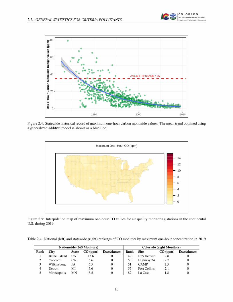
Figure 2.4 shows the trend in maximum one-hour CO values recorded statewide between 1965 and 2019. The highestone-hour concentration ever recorded at any of the state-operated monitors was 79.0 ppm, which was recorded at theDenver CAMP monitor in 1968. In 2019 the highest one-hour concentration was 2.8 ppm, a value recorded at the I-25Denver station. The one-hour annual maximum concentrations have declined from more than twice the standard in thelate 1960s to about one quarter of the standard today. Table 2.3 presents the historical maximum values recorded inColorado.

Spatial trends in maximum one-hour CO across the continental U.S. are shown in Figure 2.5. National and statewidemaximum CO values for 2019 are presented in Table 2.4.

11


Annual 8−Hr NAAQS = 9

0

10

20

30

40

1980 2000 2020

Max

8−H

our

Car

bon

Mon

oxid

e D

esig

n V

alue

s (p

pm)

CAMP

Welby

Figure 2.2: Historical record of maximum eight-hour carbon monoxide values at the CAMP and Welby stations.


0

20

40

60

80

1980 2000 2020

1−H

our

Car

bon

Mon

oxid

e D

esig

n V

alue

s (p

pm)

CAMP

Welby

Figure 2.3: Historical record of maximum one-hour carbon monoxide values at the CAMP and Welby stations.

Table 2.3: Historical maximum one-hour CO concentrations in Colorado

Site Max 1-Hour CO (ppm) YearCAMP 79.0 1968CAMP 70.0 1974CAMP 67.0 1973Denver 64.9 1979CAMP 59 1970

2019 MaximumI-25 Denver 2.8 2019

12



0

20

40

60

80

1980 2000 2020

Max

1−H

our

Car

bon

Mon

oxid

e D

esig

n V

alue

s (p

pm)

Figure 2.4: Statewide historical record of maximum one-hour carbon monoxide values. The mean trend obtained usinga generalized additive model is shown as a blue line.

Maximum One−Hour CO (ppm)

0

2

4

6

8

10

12

14

Figure 2.5: Interpolation map of maximum one-hour CO values for air quality monitoring stations in the continentalU.S. during 2019

Table 2.4: National (left) and statewide (right) rankings of CO monitors by maximum one-hour concentration in 2019

Nationwide (265 Monitors) Colorado (eight Monitors)Rank City State CO (ppm) Exceedances Rank Site CO (ppm) Exceedances1 Bethel Island CA 15.6 0 42 I-25 Denver 2.8 02 Concord CA 6.6 0 50 Highway 24 2.7 03 Wilkinsburg PA 6.5 0 51 CAMP 2.5 04 Detroit MI 5.6 0 57 Fort Collins 2.1 05 Minneapolis MN 5.5 0 82 La Casa 1.8 0

13


2.2.2 Sulfur DioxideSulfur dioxide (SO2) is one of a group of highly reactive gasses known as “oxides of sulfur,” or sulfur oxides (SOx). Thelargest sources of SO2 emissions are from fossil fuel combustion at power plants (73%) and other industrial facilities(20%), as shown in Figure 2.6. Smaller sources of SO2 emissions include industrial processes such as extracting metalfrom ore, and the burning of high sulfur containing fuels by locomotives, large ships, and non-road equipment. SO2is linked with a number of adverse effects on the respiratory system.4 Furthermore, SO2 dissolves in water and isoxidized to form sulfuric acid, which is a major contributor to acid rain, as well as fine sulfate particles in the PM2.5fraction, which degrade visibility and represent a human health hazard.

0

10000

20000

30000

1970

1975

1980

1985

1990

1991

1992

1993

1994

1995

1996

1997

1998

1999

2000

2001

2002

2003

2004

2005

2006

2007

2008

2009

2010

2011

2012

2013

2014

2015

2016

2017

2018

2019

SO

2 E

mis

sion

s (t

py)

Source Category




FUEL COMB. OTHER

HIGHWAY VEHICLES

METALS PROCESSING

MISCELLANEOUS

OFF−HIGHWAY



SOLVENT UTILIZATION

STORAGE & TRANSPORT


Figure 2.6: Trends in national sulfur dioxide emissions from 1970 to 2019.

2.2.2.1 Standards

The EPA first promulgated standards for SO2 in 1971, setting a 24-hour primary standard at 140 ppb and an annualaverage standard at 30 ppb (to protect health). A three-hour average secondary standard at 500 ppb was also adopted toprotect the public welfare. In 1996, the EPA reviewed the SO2 NAAQS and chose not to revise the standards. However,in 2010, the EPA revised the primary SO2 NAAQS by establishing a new one-hour standard at a level of 75 partsper billion (ppb). The two existing primary standards were revoked because they were deemed inadequate to provideadditional public health protection given a one-hour standard at 75 ppb.

APCD has monitored SO2 at eight locations in Colorado in the past. Currently, there are four SO2 monitoring sites inoperation. No area of the country has been found to be out of compliance with the current SO2 standards. There weretwo exceedances of the one-hour standard at the Highway 24 (Colorado Springs) site during the 2014-2015 period (seeTable 2.2); however, there was no exceedance recorded at any site in 2019.


High concentrations of sulfur dioxide can result in temporary breathing impairment for asthmatic children and adultswho are active outdoors. Short-term exposures of asthmatic individuals to elevated sulfur dioxide levels duringmoderateactivity may result in breathing difficulties that can be accompanied by symptoms such as wheezing, chest tightness, orshortness of breath. Other effects that have been associated with longer-term exposures to high concentrations of sulfurdioxide, in conjunction with high levels of particulate matter, include aggravation of existing cardiovascular disease,respiratory illness, and alterations in the lungs’ defenses. The subgroups of the population that may be affected underthese conditions include individuals with heart or lung disease, as well as the elderly and children.

4Ware, J. H., Ferris Jr, B. G., Dockery, D. W., Spengler, J. D., Stram, D. O., & Speizer, F. E. (1986). Effects of ambient sulfur oxides andsuspended particles on respiratory health of preadolescent children. The American Review of Respiratory Disease, 133(5), 834-842

14



The concentrations of sulfur dioxide in Colorado have never been a major health concern as there are few industries thatburn large amounts of coal in the state. Additionally, western coal that is mined or imported into Colorado is naturallylow in sulfur. The concern in Colorado with sulfur dioxide has been associated with acid deposition and its effects onmountain lakes and streams, as well as the formation of fine aerosols. Ambient SO2 levels have decreased significantlyin the past forty years, with one-hour SO2 annual 99th percentile values at the CAMP station having declined fromgreater than 200 ppb in the late 1960s and early 1970s to 7 ppb in 2019, as shown in Figure 2.7. Figure 2.8 showsthe declining trend in sulfur dioxide readings over the last several decades, with relatively low concentrations of sulfurdioxide recorded at APCD monitors. This same trend is evident, although not as pronounced, in the three-hour and24-hour averages. Table 2.5 presents the historical maximum one-hour concentrations recorded in Colorado. Nationaland statewide maximum values for 2019 are presented in Table 2.6.


0

100

200

300

1980 2000 2020

1−H

our

Sul

fur

Dio

xide

Des

ign

Val

ues

(ppb

)

CAMP

Welby

Figure 2.7: Historical record of one-hour sulfur dioxide annual 99th percentile values at the CAMP andWelby stations.

Table 2.5: Historical maximum one-hour SO2 concentrations in Colorado

Site Max 1-Hour SO2 (ppb) YearRio Blanco 733 1976Denver 550 1974CAMP 490 1969CAMP 360 1965Denver 328 1976

2019 MaximumHighway 24 13.9 2019

Table 2.6: National (left) and statewide (right) rankings of SO2 monitors by maximum one-hour concentration in 2019

Nationwide (467 Monitors) Colorado (four Monitors)Rank City State SO2 (ppb) Exceedances Rank Site SO2 (ppb) Exceedances1 Birmingham AL 1151 1 78 CAMP 52.2 02 New Madrid MO 442 74 126 La Casa 32.3 03 New Madrid MO 411 98 229 Welby 12.8 04 Concord CA 290 1 265 Highway 24 13.9 05 Richland TX 288 6

15



0

100

200

300

1980 2000 2020

1−H

our

Sul

fur

Dio

xide

Des

ign

Val

ues

(ppb

)

Figure 2.8: Statewide historical record of one-hour sulfur dioxide annual 99th percentile values. The mean trendobtained using a generalized additive model is shown as a blue line.

Maximum One−Hour SO2 (ppb)

0

50

100

150

200

250

300

350

400

Figure 2.9: Interpolation map of maximum one-hour SO2 values for air quality monitoring stations in the continentalU.S. during 2019

16


2.2.3 OzoneO3 is an atmospheric oxidant composed of three oxygen atoms. It is not usually emitted directly into the air, butat ground-level is formed via photochemical reactions among NOx and volatile organic compounds (VOCs) in thepresence of sunlight. Emissions from industrial facilities and electric utilities, motor vehicle exhaust, gasoline vapors,and chemical solvents are some of the major sources of NOx and VOCs (see Figure 2.10 and Figure 2.13). Breathingozone can trigger a variety of health problems, particularly for children, the elderly, and people of all ages who havelung diseases such as asthma.5 Urban areas generally experience the highest ozone concentrations, but even rural areasmay be subject to increased ozone levels because air masses can carry ozone and its precursors hundreds of miles awayfrom their original source regions.

0

10000

20000

30000

1970

1975

1980

1985

1990

1991

1992

1993

1994

1995

1996

1997

1998

1999

2000

2001

2002

2003

2004

2005

2006

2007

2008

2009

2010

2011

2012

2013

2014

2015

2016

2017

2018

2019

VO

C E

mis

sion

s (t

py)

Source Category




FUEL COMB. OTHER

HIGHWAY VEHICLES

METALS PROCESSING

MISCELLANEOUS

OFF−HIGHWAY



SOLVENT UTILIZATION

STORAGE & TRANSPORT


Figure 2.10: Trends in national VOC emissions from 1970 to 2019.

Sunlight and warm weather facilitate the ozone formation process and can lead to high concentrations. Ozone istherefore considered to be primarily a summertime pollutant and typically reaches maximum concentrations when hotsummer days provide the conditions for the precursor chemicals to react and form ozone. However, ozone can also bea wintertime pollutant in some areas. Emerging science is indicating that snow-covered oil and gas-producing basinsin the western U.S. can be subject to wintertime ozone concentrations well in excess of current air quality standards.High ozone concentrations in winter are thought to occur when stable atmospheric conditions allow for a build-up ofprecursor chemicals, and the reflectivity of the snow cover increases the rate of UV-driven reactions during the day.Ozone and its precursors are then effectively trapped under the inversion. The Upper Green River Basin in Wyominghas been studied to model such effects.6

2.2.3.1 Standards

In 1971, the EPA promulgated the first NAAQS for photochemical oxidants, setting a one-hour primary standard at 80pbb (O3 is one of a number of chemicals that are common atmospheric oxidants). The level of the primary standardwas then revised in 1979 from 80 ppb to 120 ppb and the chemical designation of the standard was changed from“photochemical oxidants” to “ozone.” In 1993, the EPA reviewed the O3 NAAQS and chose not to revise the standards.However, in 1997, the EPA promulgated a new level of the NAAQS for O3 of 80 ppb as an annual fourth-highest dailymaximum eight-hour concentration, averaged over three years. The O3 NAAQS was then revised again in 2008 whenthe EPA set an eight-hour standard of 75 ppb. OnNovember 26, 2014, the EPA again proposed lowering the O3 NAAQSstandard from 75 ppb to a level between 65 ppb and 70 ppb. In November 2015, the EPA set the standard at 70 ppb asan annual fourth-highest daily maximum eight-hour concentration, averaged over three years. To ensure compliancewith the 2008 and 2015 O3 standards, the EPA has extended the O3 monitoring requirements for Colorado by 5 months,

5Kampa, M., & Castanas, E. (2008). Human health effects of air pollution. Environmental pollution, 151(2), 362-3676Carter, W. P., & Seinfeld, J. H. (2012). Winter ozone formation and VOC incremental reactivities in the Upper Green River Basin of Wyoming.

Atmospheric Environment, 50, 255-266

17


essentially redefining Colorado’s ozone season as January through December. In 2019, seven of 21 O3 sites operatedby APCD had three-year NAAQS values in excess of the current eight-hour O3 standard of 70 ppb.


Exposure to ozone has been linked to a number of health effects, including significant decreases in lung function,inflammation of the airways, and increased respiratory symptoms, such as cough and pain when taking a deep breath.7Exposure can also aggravate lung diseases such as asthma, leading to increased medication use and increased hospitaladmissions and emergency room visits. Active children are the group at highest risk from ozone exposure becausethey often spend a large part of the summer playing outdoors. Children are also more likely to have asthma, whichmay be aggravated by ozone exposure. Other at-risk groups include adults who are active outdoors (e.g., some outdoorworkers) and individuals with lung diseases such as asthma and chronic obstructive pulmonary disease. In addition,long-term exposure to moderate levels of ozone may cause permanent changes in lung structure, leading to prematureaging of the lungs and worsening of chronic lung disease.

Ozone also affects vegetation and ecosystems, leading to reductions in agricultural crop and commercial forest yields,reduced growth and survivability of tree seedlings, and increased plant susceptibility to disease, pests, and otherenvironmental stresses (e.g., harsh weather)8. In long-lived species, these effects may become evident only afterseveral years or even decades and may result in long-term effects on forest ecosystems. Ground level ozone injury totrees and plants can lead to a decrease in the natural beauty of our national parks and recreation areas.


As illustrated in Figure 2.11, statewide average O3 values have historically fluctuated around the standard. In recentyears, the trend has been downward, but the averages seem to fluctuate within the amount of variance seen for the lastseveral years.

Ozone monitoring began in 1972 at the Denver CAMP station, and eight exceedances of the then-applicable one-hourstandard were recorded that year. Table 2.7 lists the five highest eight-hour concentrations recorded in Colorado. Notethat all five maximum historical values were recorded within the first three years of ozone monitoring. National andstatewide maximum eight-hour values for 2019 are presented in Table 2.8.


50

60

70

80

90

100

1980 1990 2000 2010 2020

8−H

our

Ozo

ne D

esig

n V

alue

s (p

pb)

Figure 2.11: Statewide historical record of eight-hour ozone NAAQS values. The mean trend obtained using ageneralized additive model is shown as a blue line.

7Lippmann, M. (1989). Health effects of ozone: a critical review. Journal of the Air Pollution Control Association, 39(5), 672-695.8Ashmore, M. R. (2005). Assessing the future global impacts of ozone on vegetation. Plant, Cell & Environment, 28(8), 949-964.

18


Table 2.7: Historical maximum eight-hour O3 concentrations in Colorado

Site Max 8-Hour O3 (ppb) YearCAMP 310 1972CAMP 264 1973Arvada 198 1973Denver 194 1973Welby 156 1974

2019 MaximumChatfield State Park 87 2019

Maximum Eight−Hour O3 (ppb)

40

50

60

70

80

90

100

Figure 2.12: Interpolation map of maximum eight-hour O3 values for air quality monitoring stations in the continentalU.S. during 2019

Table 2.8: National (left) and statewide (right) rankings of O3 monitors by maximum eight-hour concentration in 2019

Nationwide (1,236 Monitors) Colorado (21 Monitors)Rank City State O3 (ppb) Exceedances Rank Site O3 (ppb) Exceedances1 Salt Lake City UT 110 15 29 Chatfield State Park 87 92 Santa Clarita CA 105 6 53 Highland Reservoir 82 63 Fremont WY 105 9 89 NREL 79 134 Crestline CA 102 26 90 Fort Collins - West 79 45 Redlands CA 101 21 134 Welch 77 6

19


2.2.4 Nitrogen DioxideNO2 is one of a group of highly reactive gasses known as “oxides of nitrogen,” or nitrogen oxides (NOx). Other NOxspecies include nitric oxide (NO), nitrous acid (HNO2), and nitric acid (HNO3). The EPA’s National Ambient AirQuality Standard uses NO2 as the indicator for the larger group of nitrogen oxides. NO2 forms quickly from emissionsfrom motor vehicles, power plants, and off-road equipment, with on and off-road vehicles accounting for over 50% ofemissions nationally. In addition to contributing to the formation of ground-level ozone and fine particle pollution,NO2 is linked with a number of adverse effects on the respiratory system.9

0

10000

20000

1970

1975

1980

1985

1990

1991

1992

1993

1994

1995

1996

1997

1998

1999

2000

2001

2002

2003

2004

2005

2006

2007

2008

2009

2010

2011

2012

2013

2014

2015

2016

2017

2018

2019

NO

X E

mis

sion

s (t

py)

Source Category




FUEL COMB. OTHER

HIGHWAY VEHICLES

METALS PROCESSING

MISCELLANEOUS

OFF−HIGHWAY



SOLVENT UTILIZATION

STORAGE & TRANSPORT


Figure 2.13: Trends in national NOx emissions from 1970 to 2019.

2.2.4.1 Standards

The EPA first set standards for NO2 in 1971, setting both a primary standard (to protect health) and a secondary standard(to protect the public welfare) at 0.053 parts per million (53 ppb), averaged annually. The Agency has reviewed thestandards twice since that time, but chose not to revise the annual standards at the conclusion of each review. In January2010, the EPA established an additional primary standard at 100 ppb, averaged over one hour. Together the primarystandards protect public health, including the health of sensitive populations; i.e., people with asthma, children, andthe elderly.

The EPA has established requirements for an NO2 monitoring network that will include monitors at locations wheremaximumNO2 concentrations are expected to occur, including within 50meters of major roadways, as well as monitorssited to measure area-wide NO2 concentrations that occur more broadly across communities. Per these requirements,at least one monitor must be located near a major road in any urban area with a population greater than or equal to1,000,000 people. A second monitor is required near another major road in areas with either: (1) population greaterthan or equal to 2.5 million people, or (2) one or more road segments with an annual average daily traffic (AADT)count greater than or equal to 250,000 vehicles. Near-roadway monitoring is conducted at the I-25 Denver (installedin 2013) and I-25 Globeville (installed in 2015) sites. In addition to the near roadway monitoring, there must be onemonitoring station in each metropolitan area with a population of 1 million or more persons to monitor a location ofexpected highest NO2 concentrations representing the neighborhood or larger spatial scales. The CAMP site satisfiesthis requirement. Additionally, the Welby monitoring location serves as a an EPA Regional Administrated NO2 sitetargeted at the characterization of NO2 exposure for susceptible and vulnerable populations.


Elevated concentrations of nitrogen dioxide cause respiratory distress, degradation of vegetation, clothing, visibility,and increased acid deposition. Nitrogen dioxide also causes concern with the formation of fine aerosols. Nitrate

9Weinmayr, G., Romeo, E., De Sario, M., Weiland, S. K., & Forastiere, F. (2010). Short-term effects of PM10 and NO2 on respiratory healthamong children with asthma or asthma-like symptoms: a systematic review and meta-analysis. Environmental Health Perspectives, 118(4), 449-57.

20


aerosols, which result from NO and NO2 combining with water vapor in the air, have been consistently linked toDenver’s visibility problems.10


Colorado exceeded the annual mean NO2 standard of 53 ppb in 1977 at the Denver CAMP monitor, but concentrationshave shown a gradual decline since this time. Figure 2.14 and Figure 2.15 show that levels have declined minimallybut remained below the NAAQS at both the Welby and CAMP monitors over the past ten years in terms of both theannual mean and one-hour NAAQS values. The statewide historical trend is summarized in Figure 2.16. Table 2.9presents the historical maximum one-hour NO2 values recorded in Colorado. National and statewide maximum valuesfor 2019 are presented in Table 2.10.

Annual Mean NAAQS = 53

0

20

40

60

1980 2000 2020

Ann

ual M

ean

Nitr

ogen

Dio

xide

Des

ign

Val

ues

(ppb

)

CAMP

Welby

Figure 2.14: Historical record of annual mean nitrogen dioxide NAAQS values at the CAMP and Welby stations.

Table 2.9: Historical maximum one-hour NO2 concentrations in Colorado

Site Max 1-Hour NO2 (ppb) YearDenver 639 1983CAMP 620 1973CAMP 462 1989CAMP 448 1983CAMP 420 1974

2019 MaximumCAMP 86 2019

10Sloane, C. S., Watson, J., Chow, J., Pritchett, L., & Richards, L. W. (1991). Size-segregated fine particle measurements by chemical speciesand their impact on visibility impairment in Denver. Atmospheric Environment. Part A. General Topics, 25(5), 1013-1024.

21



0

100

200

300

1980 2000 2020

1−H

our

Nitr

ogen

Dio

xide

Des

ign

Val

ues

(ppb

)

CAMP

Welby

Figure 2.15: Historical record of one-hour nitrogen dioxide NAAQS values at the CAMP and Welby stations.


0

100

200

300

1980 2000 2020

1−H

our

Nitr

ogen

Dio

xide

Des

ign

Val

ues

(ppb

)

Figure 2.16: Statewide historical record of one-hour nitrogen dioxide NAAQS values. The mean trend obtained usinga generalized additive model is shown as a blue line.

Table 2.10: National (left) and statewide (right) rankings of NO2 monitors by maximum one-hour concentration in2019

Nationwide (445 Monitors) Colorado (six Monitors)Rank City State NO2 (ppb) Exceedances Rank Site NO2 (ppb) Exceedances1 Salt Lake City UT 116 1 5 CAMP 86 02 Fort Lee NJ 110 1 6 I-25 Globeville 86 03 Bethel Island NJ 107 1 8 I-25 Denver 84 04 Ryder ND 88 0 19 La Casa 74 05 Denver CO 86 0 27 Welby 67 0

22


Maximum One−Hour NO2 (ppb)

20

40

60

80

100

Figure 2.17: Interpolation map of maximum one-hour NO2 values for air quality monitoring stations in the continentalU.S. during 2019

23


2.2.5 Particulate MatterAtmospheric particulate matter (PM) consists of microscopic solid or liquid particles suspended in the air. PM can bemade up of a number of different components, including acidic aerosols (e.g., nitrates and sulfates), organic carbon,metals, soil or dust particles, and allergens (such as fragments of pollen or mold spores). Some of these particles arecarcinogenic and others have health effects due to their size, morphology, or composition.


Particle size is the factor most directly linked to the health impacts of atmospheric PM. Particles of less than 10micrometers (μm) in aerodynamic diameter (PM10) are inhalable and thus pose a health threat. Particles less than 2.5μm in aerodynamic diameter (PM2.5) can penetrate deeply into the alveoli in the lungs, while the smallest particles, suchas those less than 0.1 μm in aerodynamic diameter (ultrafine particles), can penetrate all the way into the bloodstream.Exposure to such particles can affect the lungs, the heart, and the cardiovascular system. Particles with diametersbetween 2.5 μm and 10 μm (PM10-2.5) represent less of a health concern, although they can irritate the eyes, nose, andthroat, and cause serious harm due to inflammation in the airways of people with respiratory diseases such as asthma,chronic obstructive pulmonary disease, and pneumonia. Note that PM10 encompasses all particles smaller than 10 μm,including the PM2.5 and ultrafine fractions.

The welfare effects of particulate exposure may be the most widespread of all the pollutants. No place on earth hasbeen spared from the particulate pollution generated by urban and rural sources. This is due to the potential forextremely long-range transport of fine particles and chemical reactions that occur from gases in the atmosphere tocreate secondary particulate matter in the form of microscopic liquid droplets. The effects of particulates range fromvisibility degradation to climate changes and vegetation damage. General soiling, commonly thought to be just anuisance, can have long-term adverse effects on building paints and other materials. Acid deposition as particulatescan be detected in the most remote areas of the world.

2.2.5.2 Emissions and Sources

The majority of PM10 pollution comes from miscellaneous sources, which are mainly fugitive dust sources rather thanstack emissions or combustion sources. Fugitive emissions are those not caught by a capture system and are oftendue to equipment leaks, earth moving equipment vehicles, and windblown disturbances. PM2.5, on the other hand, istypically formed in the atmosphere via gas to particle conversion and consists primarily of nitrates, sulfates, and organiccarbon (black carbon from combustion can be an important primary source of particles in the PM2.5 size fraction).Historical trends in national PM emissions from 1990 to 2019 are shown in Figure 2.18 and Figure 2.19 for illustrationpurposes.

0

10000

20000

30000

40000

1970

1975

1980

1985

1990

1991

1992

1993

1994

1995

1996

1997

1998

1999

2000

2001

2002

2003

2004

2005

2006

2007

2008

2009

2010

2011

2012

2013

2014

2015

2016

2017

2018

2019

PM

10 E

mis

sion

s (t

py)

Source Category




FUEL COMB. OTHER

HIGHWAY VEHICLES

METALS PROCESSING

MISCELLANEOUS

OFF−HIGHWAY



SOLVENT UTILIZATION

STORAGE & TRANSPORT


Figure 2.18: Trends in national PM10 emissions from 1970 to 2019.

24


0

2000

4000

6000

1990

1991

1992

1993

1994

1995

1996

1997

1998

1999

2000

2001

2002

2003

2004

2005

2006

2007

2008

2009

2010

2011

2012

2013

2014

2015

2016

2017

2018

2019

PM

2.5

Em

issi

ons

(tpy

)

Source Category




FUEL COMB. OTHER

HIGHWAY VEHICLES

METALS PROCESSING

MISCELLANEOUS

OFF−HIGHWAY



SOLVENT UTILIZATION

STORAGE & TRANSPORT


Figure 2.19: Trends in national PM2.5 emissions from 1990 to 2019.

2.2.5.3 Standards

EPA first established standards for PM in 1971. The reference method specified for determining attainment of theoriginal standards was the high-volume sampler, which collects PM up to a nominal size of 25 to 45 μm (referredto as total suspended particulates or TSP). The primary standards, as measured by the indicator TSP, were 260 μgm-3 (as a 24-hour average) not to be exceeded more than once per year, and 75 μg m-3 (as an annual geometricmean). In October 1979, the EPA announced the first periodic review of the air quality criteria and NAAQS for PM,and significant revisions to the original standards were promulgated in 1987. In that decision, the EPA changed theindicator for particles from TSP to PM10. EPA also revised the level and form of the primary standards. The EPApromulgated significant revisions to the NAAQS again in 1997. In that decision, the EPA revised the PM NAAQS inseveral respects. While it was determined that the PM NAAQS should continue to focus on particles less than or equalto 10 μm in diameter (i.e., PM10), the EPA also decided that the fine and coarse fractions of PM10 should be consideredseparately. The Agency’s decision to modify the standards was based on evidence that serious health effects wereassociated with short- and long-term exposure to fine particles in areas that met the existing PM10 standards. The EPAadded new standards, using PM2.5 as the indicator for fine particles and using PM10 as the indicator for the PM10-2.5fraction. The EPA established two new PM2.5 standards: an annual standard of 15 μg m-3, based on the 3-year averageof annual arithmetic mean PM2.5 concentrations from single or multiple community-oriented monitors, and a 24-hourstandard of 65 μg m-3, based on the 3-year average of the 98th percentile of 24-hour PM2.5 concentrations at eachpopulation-oriented monitor within an area. These standards were modified again in 2006 and 2012. The currentNAAQS for PM10 is a primary 24-hour standard of 150 μg m-3 not to be exceeded more than once per year on averageover three years. There are currently three NAAQS for PM2.5: (1) a primary annual standard of 12 μg m-3, based onthe 3-year average of annual arithmetic mean PM2.5 concentrations, (2) a secondary annual standard of 15 μg m-3,based on the 3-year average of annual arithmetic mean PM2.5 concentrations, and (3) and a 24-hour standard of 35 μgm-3, based on the 3-year average of the 98th percentile of 24-hour PM2.5 concentrations.

2.2.5.4 A Brief Explanation of Exceptional Events

Often times air pollution episodes originate from natural sources that are not preventable and cannot be reasonablycontrolled by humans. These include events like volcanic eruptions, large regional dust storms, and wildfires. If anexceedance of the NAAQS (PM10 concentrations greater than 150 μg m-3 in attainment areas and greater than 98 μgm-3 in PM10 non-attainment areas) can be shown to have resulted from a natural event and can be documented withscientific evidence, the event can be excluded from NAAQS calculations. For example, one such event was the largewind and dust storm that occurred onMarch 31, 1999whenmonitors from Steamboat Springs to Telluride reported highPM10 concentrations. Similar exceptional events have been documented in Lamar, Grand Junction, Pagosa Springs,and Pueblo. These events are not included in NAAQS determinations, not because they are without any health risk

25


but because they are naturally occurring events that cannot be reasonably prevented or controlled. The EPA mayconcur on events that APCD flags and documents as exceptional events in the EPA’s AQS database. The ExceptionalEvents Rule was revised in 2016, with an effective date of September 30, 2016. The EPA has been much morerestrictive on concurring natural events since the revision. Concentrations between 98 and 155 μg m-3 that are locatedin State Implementation Plan maintenance areas are also allowed by the Exceptional Events Rule to be flagged anddocumented as exceptional events. More details can be found at http://www.epa.gov/air-quality-analysis/treatment-data-influenced-exceptional-events/.


PM10 PM10 data have been collected in Colorado since 1985. The samplers were subsequently modified to conformto the requirements of a new standard when it was established in July of 1987. Therefore, annual trends are only validback to July 1987. Since 1988, at least one Colorado monitor has exceeded the level of the 24-hour PM10 standard(150 μg m-3) every year except for 2004.

In cases other than exceptional events and more so than for other pollutants, PM10 pollution is a localized phenomenonand concentrations can vary considerably in Colorado on both spatial and temporal scales. Therefore, local averagesand maximum concentrations of PM10 are more meaningful than averages covering large regions or the entire state.However, statewide values have been summarized in a box plot in Figure 2.20 for illustration purposes. The box plotshows the median PM10 NAAQS value statewide for each year as a horizontal black bar, as well as the first quartile(Q1, box bottom), the third quartile (Q3, box top), and the minimum and maximum values, which are representedby vertical black tick marks. For each year, outliers are considered to be those points with values greater than Q3 +1.5*(Q3 - Q1) or less than Q1 - 1.5*(Q3 - Q1), and are represented by black points. Maximum historical values greaterthan 500 μg m-3 are labeled in in Figure 2.20 with the name of the city where those values were measured.

The data shown in Figure 2.20 include those concentrations that are the result of exceptional events (see subsubsec-tion 2.2.5.4). There have been several of these events documented in Colorado since PM10 monitoring began in 1987,including the maximum 24-hour PM10 concentration of 1220 μg m-3 recorded in Lamar in 2013 and the 635 μg m-3

value recorded in Alamosa in 2011. Table 2.11 presents the historical maximum 24-hour PM10 concentrations recordedin Colorado.

National and statewide maximum 24-hour PM10 concentrations for 2019 are presented in Table 2.12. In the pastseveral years the top five locations on the list have generally included Keeler, CA, sites around Owens Lake, CA, andsites around Mono Lake, CA. All of these levels are associated with hot dry winds. The levels around Owens Lake areassociated with high winds that blow across a large dry lake bed. In the past, several monitors in that area have recordedlevels in excess of 20,000 μg m-3 as a 24-hour average. Exceedances in Colorado are mainly due to large regional duststorms that usually begin in desert areas to the south and west of the state. These are natural or exceptional eventsfor which the Division is currently analyzing the scientific data and documenting as high wind/blown dust exceptionalevents.

Spatial trends in median 24-hour PM10 across the continental U.S. are shown in Figure 2.21. By plotting the medianinstead of maximum values, the effect of exceptional event data is effectively removed from this plot.

Table 2.11: Historical maximum 24-hour PM10 concentrations in Colorado

Site Max 24-Hour PM10 (μg m-3) YearLamar 1,220 2013Alamosa 635 2011Denver 532 1985Alamosa 494 2007Montrose 491 1999

2019 MaximumSteamboat Springs 228 2019

26

http://www.epa.gov/air-quality-analysis/treatment-data-influenced-exceptional-events/

http://www.epa.gov/air-quality-analysis/treatment-data-influenced-exceptional-events/


●

●

●●●

●

●

●

●

●

●

● ●●

●

●

●

● ●●

●●

●

●

●

●●

● ●

●

●●

●●

●●●

●

●●

●

●●●

●●

●●●

●●

●●●

●

●

●

●

●●

●

●

●

●●

●

●●

●

●

●●

●

●●

●

●

●

●

●

●

●

●●

●

●

●

●

●

●

●

●

●

●

●

●●

●

●

Annual Max 24−Hour NAAQS = 150

0

250

500

750

1000

1250

1990 2000 2010 2020

Max

24−

Hou

r P

M10

Des

ign

Val

ues

(µg

m−

3 )

Figure 2.20: Statewide historical record of annual maximum 24-hour PM10 values. The box plot shows the medianPM10 NAAQS value statewide for each year, as well as the interquartile range (box) of values observed at monitoringsites throughout the state and the minimum and maximum values. Outliers are indicated by black points.

Median 24−Hour PM10 (µg m−3)

5

10

15

20

25

30

35

40

45

Figure 2.21: Interpolation map of median 24-hour PM10 values for air quality monitoring stations in the continentalU.S. during 2019

Table 2.12: National (left) and statewide (right) rankings of PM10 monitors by maximum 24-hour concentration in2019

Nationwide (708 Monitors) Colorado (15 Monitors)Rank City State PM10 (μg m-3) Exceedances Rank Site PM10 (μg m-3) Exceedances1 Mono Lake CA 3,956 9 22 Steamboat Springs 228 12 Ak-Chin Village AZ 990 11 76 TCH 119 03 Sunland Park NM 734 6 84 Lamar 105 04 Deming NM 721 2 129 Pueblo 89 05 Organ NM 691 3 149 CAMP 79 0

27


PM2.5 Monitoring for PM2.5 in Colorado began in 1999 with the establishment of sites in Denver, Grand Junction,Steamboat Springs, Colorado Springs, Greeley, Fort Collins, Platteville, Boulder, Longmont, and Elbert County.Additional sites were established nearly every month until full implementation of the base network was achieved inJuly of 1999. In 2004, there were 20 PM2.5 monitoring sites in Colorado. Thirteen of the 20 sites were selectedbased on the population of the metropolitan statistical areas. This is a federal selection criterion that was developed toprotect the public health in the highest population centers. In addition, there were seven special-purpose-monitoring(SPM) sites. These sites were selected due to historically elevated concentrations of PM10 or because citizens or localgovernments had concerns about possible high PM2.5 concentrations in their communities. A majority of the SPMsites were removed as of December 31, 2006 due to low concentrations and a lack of funding.

Figure 2.22 and Figure 2.23 show the historical trends in annual mean and 24-hour maximum PM2.5 NAAQS values,respectively. Although data has only been collected for the past 21 years, the trend in the average levels of PM2.5appears to be essentially flat. Since the 35 μg m-3 standard is based on a three-year average of the 98th percentile, the24-hour standard has not been violated at any site for 2019, nor has the three-year average annual standard of 12 μgm-3. Table 2.13 presents the historical maximum 24-hour PM2.5 concentrations recorded in Colorado. National andstatewide maximum 24-hour PM2.5 concentrations for 2019 are presented in Table 2.6.

98th Percentile NAAQS = 35

10

20

30

40

50

2000 2005 2010 2015 2020

98th

Per

cent

ile P

M2.

5 D

esig

n V

alue

s (µ

g m

−3 )

Figure 2.22: Statewide historical record of 24-hour PM2.5 98th percentile values. The mean trend obtained using ageneralized additive model is shown as a blue line.

Table 2.13: Historical maximum 24-hour PM2.5 concentrations in Colorado

Site Max 24-Hour PM2.5 (μg m-3) YearArapahoe Community College (ACC) 140 1999Fort Collins - CSU 75 2015CAMP 68 2001Chatfield State Park 62 2017Greeley 62 2017

2019 MaximumLa Casa 59 2019

28


Annual Mean NAAQS = 12

5

10

15

2000 2005 2010 2015 2020

Ann

ual M

ean

PM

2.5

Con

cent

ratio

n (µ

g m

−3 )

Figure 2.23: Statewide historical record of annual mean PM2.5 values. The mean trend obtained using a generalizedadditive model is shown as a blue line.

Maximum 24−Hour PM2.5 (µg m−3)

0

10

20

30

40

50

60

70

80

Figure 2.24: Interpolation map of maximum 24-hour PM2.5 values for air quality monitoring stations in the continentalU.S. during 2019

Table 2.14: National (left) and statewide (right) rankings of PM2.5 monitors by maximum 24-hour concentration in2019

Nationwide (960 Monitors) Colorado (17 Monitors)Rank City State PM2.5 (μg m-3) Exceedances Rank Site PM2.5 (μg m-3) Exceedances1 Madawaska ME 99 2 14 La Casa 59 12 Houston TX 91 1 16 I-25 Globeville 57 23 Bakersfield CA 84 1 19 CAMP 53 14 Berks PA 83 4 23 Chatfield State Park 53 15 Liberty PA 76 5 26 I-25 Denver 52 1

29

3

Non-Criteria Pollutants

Non-criteria pollutants are those pollutants for which there are no current national ambient air quality standards. Theseinclude but are not limited to visibility, certain oxides of nitrogen species, total suspended particulates, some continuousparticulate monitoring, and air toxics. Meteorological measurements of wind speed, wind direction, temperature, andhumidity are also included in this group, as is chemical speciation of PM2.5.

3.1 VisibilityVisibility is unique among air pollution effects in that it involves human perception and judgment. It has been describedas the maximum distance that an object can be perceived against the background sky. Visibility also refers to the claritywith which the form and texture of distant, middle, and near details can be seen as well as the sense of the trueness oftheir apparent coloration. As a result, measures of visibility serve as surrogates of human perception. There are severalways to measure visibility but none of them tell the whole story or completely measure visibility as we experienceit.

3.1.1 StandardsThe Colorado Air Quality Control Commission established a visibility standard in 1990 for the Denver Metropolitan“AIR Program” area. The standard, an atmospheric extinction of 0.076 per inverse kilometer, was based on the public’sdefinition of unacceptable amounts of haze as judged from slides of different haze levels taken in the Denver area. Atthe standard, 7.6% of the light is extinguished in each kilometer of air, and the standard is violated when the four-houraverage extinction exceeds 7.6%. The standard applies from 8 A.M. to 4 P.M. each day, during those hours whenthe relative humidity is less than 70%. Visibility, along with meteorology and concentrations of other pollutants forwhich National Ambient Air Quality Standards exist, is used to determine the need for mandatory wood burning andvoluntary driving restrictions.

There is no quantitative visibility standard for Colorado’s pristine and scenic rural areas. However, in the 1977amendments to the Federal Clean Air Act, Congress added Section 169a (Clean Air Act as amended in 1977, Section169a 1977) and established a national visibility goal that created a qualitative standard of “the prevention of any future,and the remedying of any existing, impairment of visibility in mandatory Class I federal areas which impairment resultsfrom man-made air pollution.” The implementation of Section 169a has led to federal requirements to protect visualair quality in large national parks and wilderness areas (Visibility Protection for Federal Class 1 Areas n.d.). Twelve ofthese Class I areas are located in Colorado. Federal and state law prohibits visibility impairment in national parks andwildernesses due to large stationary sources of air pollution.

3.1.2 Impacts on Public WelfareVisual air quality is an element of public welfare. Specifically, it is an important aesthetic, natural, and economicresource of the State of Colorado. EPA, the US Forest Service, and the US National Park Service have conducted

30

3.1. VISIBILITY

studies that show that good visibility is something that people undeniably value. They have also shown that impairedvisibility affects the enjoyment of a recreational visit to a scenic mountain area.

While the value of visibility is difficult to measure, APCD believes that people prefer to have clear views from theirhomes and offices. These concerns are reflected in residential property values and office rents. Any loss in visualair quality may contribute to corresponding losses in tourism and usually make an area less attractive to residents,potential newcomers, and industry. Researchers have found this link strongest with concentrations of fine particles,which are the main contributor to visibility impairment. In July 1997, the EPA developed a NAAQS for PM2.5 (moredetails are in subsubsection 2.2.5.3). Any control strategies to lower ambient concentrations of fine particulate matterfor health reasons will also improve visibility.

3.1.3 SourcesThe cause of visibility impairment in Colorado is most often fine particles in the 0.1 to 2.5 μm size range. Lightpassing from a vista to an observer is either scattered away from the sight path or absorbed by the atmospheric fineparticulates. Sunlight entering the pollution cloud may be scattered into the sight path adding brightness to the viewand making it difficult to see elements of the vista. Sulfate, nitrate, elemental carbon, and organic carbon are the typesof particulate matter most effective at scattering and/or absorbing light. The man-made sources of these particulatesinclude wood burning, electric power generation, industrial combustion of coal or oil, and emissions from cars, trucks,and buses.

Visibility conditions vary considerably across the state. Usually, visibility in Colorado is among the best in the country.Our prized western vistas exist due to unique combinations of topography and scenic features. Air in much of the Westcontains low humidity and minimal levels of visibility-degrading pollution. Nevertheless, visibility problems occurperiodically throughout the state. Wood burning haze is a concern in several mountain communities each winter andDenver has its “Brown Cloud” pollution episodes.1 Even national parks, monuments, and wilderness areas experiencepollution related visibility impairment on occasion due to regional haze, interstate traffic or even regional or global-scale transport of visibility-degrading pollution.2 The visibility problems across the state have raised public concernand spurred research. The goal of Colorado’s visibility program is to protect visual air quality where it is presentlyacceptable and improve visibility where it is degraded.

3.1.4 Class I Areas in ColoradoPhase 1 of the visibility program, also known as Reasonably Attributable Visibility Impairment (RAVI), addressesimpacts in Class I areas by establishing a process to evaluate source specific visibility impacts, or plume blight, fromindividual sources or small groups of sources. Figure 3.1 illustrates these areas in Colorado.

Section 169Bwas added to the Clean Air Act Amendments of 1990 to address Regional Haze. Since Regional Haze andvisibility problems do not respect state and tribal boundaries, the amendments authorized EPA to establish visibilitytransport regions as a way to combat regional haze.

Phase 2 of the visibility program addresses Regional Haze. This form of visibility impairment focuses on overalldecreases in visual range, clarity, color, and ability to discern texture and details in Class I areas. The responsible airpollutants can be generated in the local vicinity or carried by the wind often many hundreds or even thousands of milesfrom where they originated.

APCD developed a Regional Haze State Implementation Plan (SIP) in 2010 illustrating how Colorado intends to meetthe requirements of EPA’s Regional rules for the period ending in 2018 (the first planning period in the rule), while alsoestablishing enforceable controls that will help address the long term national visibility goals targeted to be achievedby the year 2064.

Colorado’s Regional Haze SIP was approved by the Colorado Air Quality Control Commission on January 7, 2011.This plan will lead to less haze and improved visibility in some of Colorado’s most treasured and scenic areas, including

1Neff, W. D. (1997). The Denver Brown Cloud studies from the perspective of model assessment needs and the role of meteorology. Journal ofthe Air & Waste Management Association, 47(3), 269-285

2Kavouras, I. G., Etyemezian, V., DuBois, D. W., Xu, J., & Pitchford, M. (2009). Source reconciliation of atmospheric dust causing visibilityimpairment in Class I areas of the western United States. Journal of Geophysical Research: Atmospheres (1984-2012), 114(D2)

31

3.1. VISIBILITY

Weminuche Wilderness

Rocky Mountain NP

Flat Tops Wilderness

West Elk Wilderness

Mount Zirkel Wilderness

La Garita Wilderness

Eagles Nest Wilderness

Maroon Bells-Snowmass Wilderness

Rawah Wilderness

Mesa Verde NP

Great Sand Dunes Wilderness

Black Canyon of the Gunnison Wilderness

Ü

0 60 12030 Miles Forest Service

National Park Service

Figure 3.1: Class I areas in Colorado shown in green and blue. Blue indicates a National Park or Preserve, and greenindicates a federally-protected wilderness area.

Rocky Mountain National Park, Mesa Verde, Maroon Bells, and the Great Sand Dunes. By 2018, the plan will resultin more than 70,000 tons of pollutant reductions annually, including 35,000 tons of nitrogen oxides, which leads toground-level ozone formation. In total, the plan covers 30 industrial emitters at 16 facilities throughout Colorado,including coal-fired power plants and cement kilns.

3.1.5 MonitoringThere are several ways to measure visibility. APCD uses camera systems to provide qualitative visual documentationof a view. Transmissometers and nephelometers are used to measure the atmosphere’s ability to attenuate lightquantitatively.

A visibility site was installed in Denver in late 1990 using a long-path transmissometer. Visibility in the downtownarea is monitored using a receiver located near Cheesman Park at 1901 E. 13th Avenue and a transmitter located on theroof of the Federal Building at 1929 Stout Street (Figure 3.2). This instrument directly measures light extinction, whichis proportional to the ability of atmospheric particles and gases to attenuate image-forming light as it travels from anobject to an observer. The visibility standard is stated in units of atmospheric extinction. Days when the visibility isaffected by rain, snow, or relative humidity above 70% are termed “excluded” and are not counted as violations of thevisibility standard.

Elsewhere in Colorado, several agencies of the federal government, in cooperation with regional and nationwide stateair pollution organizations, also monitor visibility in a number of national parks and wilderness Class I areas, eitherindividually or jointly through the Interagency Monitoring of Protected Visual Environments (IMPROVE) program.The goals of the monitoring programs are to establish background visibility levels, identify trends of deteriorationor improvement, identify suspected sources of visibility impairment, and to track regional haze. Visibility and theatmospheric constituents that cause visibility degradation are characterized with camera systems, transmissometers,and extensive fine particle chemical composition measurements by the monitoring network. There are currentlyIMPROVE monitoring sites in Rocky Mountain National Park, Mesa Verde National Park, Weminuche Wilderness,Mount Zirkel Wilderness, Great Sand Dunes National Monument, White River National Forest, San Juan NationalForest, and Flattops Wilderness. These data are not contained in this report, but are available at http://vista.cira.colostate.edu/improve/.

32

http://vista.cira.colostate.edu/improve/

http://vista.cira.colostate.edu/improve/

3.1. VISIBILITY

Figure 3.2: Denver transmissometer path (for illustration purposes only).

3.1.6 Denver CameraAPCD operates a web-based camera that can be viewed on the Live Image of Denver icon on the bottom left side of thescreen at the APCD web site http://www.colorado.gov/airquality. There is a great deal of other informationavailable from this site in addition to the image from the visibility camera, including the Front Range Air QualityForecast, Air Quality Advisory, Monitoring Reports, this report, and Open Burning Forecast.

The images in Figure 3.3 show the visibility on one of the best and one of the worst days for the year, December 18thand February 26th, respectively.

Figure 3.3: Denver Camera images of the best (left) and worst (right) visibility days in Denver during 2019.

These two pictures are images made by the web camera at the visibility monitor located at 1901 E. 13th Avenuein Denver, and are centered on the Federal Building at 1929 Stout Street (see Figure 3.2, the camera follows thetransmissometer path). The difference in these two pictures is not just the brightness but the detail that can be seenbetween the two images. On the best day, buildings can be clearly resolved, and the Front Range is visible. On theworst day, however, contrast between buildings is lower, and the Front Range is obscured.

33

http://www.colorado.gov/airquality

3.2. NITRIC OXIDE

3.2 Nitric OxideNitric oxide (NO) is the most abundant of the oxides of nitrogen emitted from combustion sources. There are no knownadverse health effects at normal ambient concentrations. However, NO is a precursor to nitrogen dioxide, nitric acid,particulate nitrates, and ozone, all of which have demonstrated adverse health effects. There are no federal or statestandards for nitric oxide.

Nitric oxide was measured simultaneously with NO2 at the Welby, CAMP, La Casa, I-25 Globeville, I-25 Denver,and Rocky Flats sites. Table 3.1 shows the maximum and average NO concentrations measured in Colorado in 2019.Without national standards with which to compare these numbers, they are presented here for informational purposesonly, and are considered by APCD to be consistent with recent historical nitric oxide concentrations.

Table 3.1: Summary of average and maximum one-hour nitric oxide values measured at APCD monitoring sites in2019.

Site Name County NO (ppb)Annual Average Maximum Value

Welby Adams 13.8 253CAMP Denver 13.4 332La Casa Denver 11.1 240I-25 Denver Denver 26.9 314I-25 Globeville Denver 34.7 340Rocky Flats - N. Jefferson 0.7 22

3.3 Air ToxicsToxic air pollutants, or air toxics, are those pollutants that cause or may cause cancer or other serious health effects, suchas reproductive effects or birth defects. Air toxics may also cause adverse environmental and ecological effects. EPAis required to reduce air emissions of 188 air toxics listed in the Clean Air Act. Examples of air toxics include benzene(found in gasoline), perchloroethylene (emitted from some dry cleaning facilities), and methylene chloride (used as asolvent by a number of industries). Most air toxics originate from man-made sources, including mobile sources likecars, trucks, and construction equipment, and stationary sources like factories, refineries, and power plants, as well asindoor sources (some building materials and cleaning solvents). Some air toxics are also released from natural sourcessuch as volcanic eruptions and forest fires (United States Environmental Protection Agency 2009).

People exposed to air toxics at sufficient concentrations may experience various health effects including cancer anddamage to the immune system, as well as neurological, reproductive (including reduced fertility), developmental,respiratory, and other health problems. In addition to exposure from breathing air toxics, risks are also associatedwith the deposition of toxic pollutants onto soils or surface waters, where they are taken up by plants and ingested byanimals and eventually magnified up through the food chain. Like humans, animals may experience health problemsdue to air toxics exposure.

Since 2004, APCD has monitored air toxics in Grand Junction as part of EPA’s National Air Toxics Trend Stationsproject. Monitoring for ozone precursors, which are a subset of air toxics, began at CAMP and Platteville in Decemberof 2011. The data from the Grand Junction study and the Ozone Precursor study are available in separate reports,available at http://www.colorado.gov/airquality/tech.aspx.

3.4 MeteorologyAPCD takes a limited set ofmeteorologicalmeasurements at 18 locations around the state. Thesemeasurements includewind speed, wind direction, temperature, standard deviation of horizontal wind direction, and select monitoring ofrelative humidity, atmospheric pressure, and solar radiation. Relative humidity measurements are also taken inconjunction with the two visibility monitors. The humidity data are not summarized in this report since they are usedprimarily to validate the visibility measurements taken at the specific locations. The Division also began collecting

34

http://www.colorado.gov/airquality/tech.aspx

3.5. CHEMICAL SPECIATION OF PM2.5

precipitation measurements at the Rocky Flats North site in 2019. The wind speed, wind direction, and temperaturemeasurements are collected primarily for air quality forecasting and air quality modeling. These instruments areinstalled on ten-meter towers and the data are collected as hourly averages and sent along with other air quality datato be stored on the EPA’s Air Quality Systems database. The wind speed and wind direction data are shown as windroses at the end of each monitoring area in chapter 4 below.

The wind roses displayed in this report (see chapter 4) are based on the direction that the wind is blowing from. Anotherway of visualizing a wind rose is to picture yourself standing in the center of the plot and facing into the wind. Thewind direction is divided into 12 cardinal directions (ESE, for example). The wind speed is divided into six ranges.The roses in Section 4 below use 0-2 ms-1, 2-4 ms-1, 4-6 ms-1, 6-8 ms-1, 8-10 ms-1, and greater than 10 ms-1. Thelength of each arm of the wind rose represents the percentage of time the wind was blowing from that direction at thatspeed. The longer the arm, the greater the percentage of time the wind is blowing from that direction.

3.5 Chemical Speciation of PM2.5Numerous health effects studies have correlated negative health effects to the total mass concentration of PM2.5 inambient air. However, it has not yet been completely determined if the health correlation is to total mass concentration,or to concentrations of specific chemical species in the PM2.5 mix. When the EPA promulgated the NAAQS for PM2.5in 1997, a compliance monitoring network based on total PM2.5 mass was established. Mass concentrations from thecompliance network are used to determine attainment of the NAAQS. EPA soon supplemented the PM2.5 network withthe Speciation Trends Network (STN) monitoring to provide information on the chemical composition of PM2.5. Themain purpose of the STN is to identify sources, develop implementation plans to reduce PM2.5 pollution, and supporthealth effects research.

Colorado began chemical speciation monitoring at the Commerce City site in February 2001. Four other chemicalspeciation sites were established in 2001 in Colorado Springs, Durango, Grand Junction, and Platteville. The Durangosite was closed in September 2003. The Colorado Springs site was closed in December 2006. These sites wereeliminated when concentrations were found to trend low and when funding was reduced for the project. The GrandJunction site was closed in December 2009 and moved to DMAS NCore where it began sampling in January of 2010to comply with the requirement from EPA to monitor PM2.5 speciation at NCore sites. The DMAS NCore site wasshut down due to redevelopment of the property and moved to the La Casa NCore monitoring site at 4545 NavajoStreet in late 2012. APCD is currently monitoring for PM2.5 speciation at the LaCasa, Platteville and Commerce Citymonitoring sites.

If PM2.5 pollution is to be controlled, it is important to know the composition of PM2.5 particles so that the appropriatesources can be targeted for reductions (see subsubsection 2.2.5.3 above for more information on PM2.5 sources).Therefore, chemical speciation monitoring is conducted for 47 elemental metals, five ionic species, and elemental andorganic carbon. Selected filters can also be analyzed for semi-volatile organics and microscopic analyses. The resultsof these samples can be obtained from APCD upon request. Some of these chemical species and compounds cancause serious health effects, premature death, visibility degradation, and regional haze. The chemical speciation datafor PM2.5 is used in many ways, such as to determine which general source categories are likely responsible for thePM2.5 pollution at a given monitoring site on a given day, and how much pollution comes from each source category.There are two broad categories of PM2.5 - primary and secondary particles. Primary PM2.5 particles include thoseemitted directly to the air. Primary particles include carbonaceous particles from incomplete combustion in internalcombustion engines, wood burning appliances, waste burning, and crushed geologic materials. Secondary PM2.5is formed from gases that combine in the atmosphere through chemical processes and form liquid aerosol droplets.Ammonium nitrates and ammonium sulfates are generally the two largest types of secondary PM2.5 in Colorado.

35

4

Spatial Variability of Air Quality

In this section, concentration data covering the last fifteen years are summarized for each air quality monitor inthe APCD network, which are grouped below by monitoring region and pollutant. The plots in this section showannual means and one-hour, eight-hour, or 24-hour values in the form of the NAAQS standards. The values recordedat individual sites are compared to statewide averages, which are shown in light blue in all plots. Please refer tosubsection 1.1.2 for a brief description of the monitoring regions discussed below.

4.1 Central Mountains Region

4.1.1 Particulate MatterThere was one violation of the PM10 NAAQS in the Central Mountain region during 2019. The maximum 24-hourconcentration of 228 μg m-3 was recorded at the Steamboat Springs site on April 1. This exceedance was due to dustfrom sweeping an adjacent parking lot and has been discussed with the city. The second highest 24-hour average PM10concentration recorded at this site in 2019 was 73 μg m-3. The Cañon City PM10 monitor did not meet completenessrequirements during 2019 and so does not have a valid three-year design value.

Table 4.1: Summary of PM10 values recorded at monitoring stations in the Central Mountains region during 2019.

Site Name County PM10 (μg m-3)Annual Average 24-Hr Max 3-Year Exceedances

Cañon City Fremont 14.8 31 -Aspen Pitkin 12.3 50 0Steamboat Springs Routt 16.6 228 0.3

36

4.1. CENTRAL MOUNTAINS REGION

Statewide Average0

50

100

150

200

2004 2008 2012 2016

Max

24−

Hou

r P

M10

Val

ues

(µg

m−3

)

Central Mountains Region

Statewide Average0

10

20

2004 2008 2012 2016

Mea

n P

M10

(µg

m−3

)

Aspen Cañon City Steamboat Springs

Figure 4.1: Fifteen-year trend in maximum 24-hour PM10 values (top) and annual mean concentrations (bottom) formonitoring sites in the Central Mountains region. The 24-hour NAAQS (150 μg m-3) is shown as a dashed red line.

37

4.2. DENVER METRO / NORTH FRONT RANGE REGION

4.2 Denver Metro / North Front Range Region

4.2.1 Particulate MatterThere were no violations of the PM10 NAAQS in the Denver Metro/North Front Range region during 2019; however,several sites recorded 24-hour average values in exceedance of the 24-hour PM2.5 standard of 35 μg m-3, includingTri County Health, Longmont, CAMP, NJH, La Casa, I-25 Denver, I-25 Globeville, Chatfield State Park, Fort CollinsCSU, and Greeley - Hospital. The tables below list the PM10 and PM2.5 annual averages and design values recordedat each site in this region in 2019. The NJH PM2.5 monitor has only been in operation since 2018, so the three-yeardesign value is not valid for this site.

The PM2.5 plots below show the 98th percentile of the data collected during each year rather than the three-yearaverage.

Table 4.2: Summary of PM10 values recorded at monitoring stations in the Denver Metro/Northern Front Range regionduring 2019.


Tri-County Adams 34.6 119 0.3Welby Adams 30.7 90 0Longmont Boulder 20.9 58 0Boulder Chamber of Comm. Boulder 23.8 53 0CAMP Denver 29.9 79 0La Casa Denver 22.2 61 0

Statewide Average0

50

100

150

2004 2008 2012 2016

Max

24−

Hou

r P

M10

Val

ues

(µg

m−3

)

Denver Metro/North Front Range Region

Statewide Average0

10

20

30

2004 2008 2012 2016

Mea

n P

M10

(µg

m−3

)

Boulder − CC CAMP La Casa Longmont TCH Welby

Figure 4.2: Fifteen-year trend in maximum 24-hour PM10 values (top) and annual mean concentrations (bottom) formonitoring sites in the Denver Metro/Northern Front Range region. The 24-hour NAAQS (150 μg m-3) is shown as adashed red line.

38


Table 4.3: Summary of PM2.5 values recorded at monitoring stations in the Denver Metro/Northern Front Range regionduring 2019.

Site Name County PM2.5 (μg m-3)

Annual Average Annual98th Percentile

3-Year Ave. of98th Percentile

Tri-County Adams 9.0 22.6 25Arapaho Comm. College Arapahoe 6.0 26.6 22Longmont Boulder 7.4 35.7 28Boulder Chamber of Comm. Boulder 5.8 19.0 19CAMP Denver 7.0 23.8 21National Jewish Health Denver 7.5 23.7 -La Casa Denver 7.5 22.0 21I-25 Denver Denver 8.1 23.0 23I-25 Globeville Denver 10.0 28.9 25Chatfield State Park Douglas 6.2 25.1 30Fort Collins - CSU Larimer 6.0 19.7 19Greeley - Hospital Weld 9.0 25.7 24Platteville Weld 7.3 22.9 20

Statewide Average0

10

20

30

2004 2008 2012 2016

98th

Per

cent

ile P

M2.

5 V

alue

s (µ

g m

−3)

Denver Metro/North Front Range Region: Adams County

Statewide Average0.0

2.5

5.0

7.5

10.0

12.5

2004 2008 2012 2016

Ann

ual M

ean

PM

2.5

(µg

m−3

)

TCH

Figure 4.3: Fifteen-year trend in 24-hour PM2.5 annual 98th percentile values (top) and annual mean concentrations(bottom) for monitoring sites in Adams County. The 24-hour and annual mean NAAQS (35 μg m-3 and 12 μg m-3,respectively) are shown as dashed red lines.

39


Statewide Average0

10

20

30

2004 2008 2012 2016

98th

Per

cent

ile P

M2.

5 V

alue

s (µ

g m

−3)

Denver Metro/North Front Range Region: Arapahoe County


2.5

5.0

7.5

10.0

12.5

2004 2008 2012 2016

Ann

ual M

ean

PM

2.5

(µg

m−3

)

ACC

Figure 4.4: Fifteen-year trend in 24-hour PM2.5 annual 98th percentile values (top) and annual mean concentrations(bottom) for monitoring sites in Arapahoe County. The 24-hour and annual mean NAAQS (35 μg m-3 and 12 μg m-3,respectively) are shown as dashed red lines.

40


Statewide Average0

10

20

30

2004 2008 2012 2016

98th

Per

cent

ile P

M2.

5 V

alue

s (µ

g m

−3)

Denver Metro/North Front Range Region: Boulder County


2.5

5.0

7.5

10.0

12.5

2004 2008 2012 2016

Ann

ual M

ean

PM

2.5

(µg

m−3

)

Boulder − CC Longmont

Figure 4.5: Fifteen-year trend in 24-hour PM2.5 annual 98th percentile values (top) and annual mean concentrations(bottom) for monitoring sites in Boulder County. The 24-hour and annual mean NAAQS (35 μg m-3 and 12 μg m-3,respectively) are shown as dashed red lines.

41


Statewide Average0

10

20

30

2004 2008 2012 2016

98th

Per

cent

ile P

M2.

5 V

alue

s (µ

g m

−3)

Denver Metro/North Front Range Region: Denver County

Statewide Average0

5

10

2004 2008 2012 2016

Ann

ual M

ean

PM

2.5

(µg

m−3

)

CAMP I−25: Denver I−25: Globeville La Casa NJH

Figure 4.6: Fifteen-year trend in 24-hour PM2.5 annual 98th percentile values (top) and annual mean concentrations(bottom) for monitoring sites in Denver County. The 24-hour and annual mean NAAQS (35 μg m-3 and 12 μg m-3,respectively) are shown as dashed red lines.

42


Statewide Average0

10

20

30

2004 2008 2012 2016

98th

Per

cent

ile P

M2.

5 V

alue

s (µ

g m

−3)

Denver Metro/North Front Range Region: Douglas County


2.5

5.0

7.5

10.0

12.5

2004 2008 2012 2016

Ann

ual M

ean

PM

2.5

(µg

m−3

)

Chatfield

Figure 4.7: Fifteen-year trend in 24-hour PM2.5 annual 98th percentile values (top) and annual mean concentrations(bottom) for monitoring sites in Douglas County. The 24-hour and annual mean NAAQS (35 μg m-3 and 12 μg m-3,respectively) are shown as dashed red lines.

43


Statewide Average0

10

20

30

2004 2008 2012 2016

98th

Per

cent

ile P

M2.

5 V

alue

s (µ

g m

−3)

Denver Metro/North Front Range Region: Larimer County


2.5

5.0

7.5

10.0

12.5

2004 2008 2012 2016

Ann

ual M

ean

PM

2.5

(µg

m−3

)

Fort Collins − CSU

Figure 4.8: Fifteen-year trend in 24-hour PM2.5 annual 98th percentile values (top) and annual mean concentrations(bottom) for monitoring sites in Larimer County. The 24-hour and annual mean NAAQS (35 μg m-3 and 12 μg m-3,respectively) are shown as dashed red lines.

44


Statewide Average0

10

20

30

2004 2008 2012 2016

98th

Per

cent

ile P

M2.

5 V

alue

s (µ

g m

−3)

Denver Metro/North Front Range Region: Weld County


2.5

5.0

7.5

10.0

12.5

2004 2008 2012 2016

Ann

ual M

ean

PM

2.5

(µg

m−3

)

Greeley − Hospital Platteville

Figure 4.9: Fifteen-year trend in 24-hour PM2.5 annual 98th percentile values (top) and annual mean concentrations(bottom) for monitoring sites in Weld County. The 24-hour and annual mean NAAQS (35 μg m-3 and 12 μg m-3,respectively) are shown as dashed red lines.

45


4.2.2 Carbon Monoxide

Table 4.4: Summary of CO values recorded at monitoring stations in the Denver Metro / Northern Front Range regionduring 2019.

Site Name CountyCO 1-Hour

Average (ppm)CO 8-Hour

Average (ppm)1st Max. 2nd Max. 1st Max. 2nd Max.

Welby Adams 1.8 1.7 1.4 1.3CAMP Denver 2.5 2.4 1.9 1.6La Casa Denver 1.8 1.7 1.3 1.3I-25 Denver Denver 2.8 2.6 2.1 2.0Fort Collins - Mason Larimer 2.1 2.1 1.5 1.3Greeley - County Tower Weld 1.3 1.3 1.0 0.8

46


Statewide Average0

10

20

30

2004 2008 2012 2016

Max

1−H

our

CO

Val

ues

(ppm

)



2.5

5.0

7.5

2004 2008 2012 2016

Max

8−H

our

CO

Val

ues

(ppm

)


0.2

0.4

0.6

2004 2008 2012 2016

Mea

n C

O (

ppm

)

CAMP Fort Collins Greeley I−25: Denver La Casa Welby

Figure 4.10: Fifteen-year trend in annual maximum one-hour (top) and eight-hour (center) CO values and annual meaneight-hour CO concentrations (bottom) for monitoring sites in the Denver Metro/Northern Front Range region. Theone-hour and eight-hour NAAQS (35 ppm and 9 ppm, respectively) are shown as dashed red lines.

47


4.2.3 OzoneThe Boulder Reservoir site has only been in operation since September 2016, so three-year NAAQS values are notvalid for these sites. The Aspen Park monitoring site was closed on 9/15/2019.

Table 4.5: Summary of O3 values recorded at monitoring stations in the Denver Metro / Northern Front Range regionduring 2019. Sites having three-year NAAQS values in excess of 70 ppb are indicated by asterisks.

Site Name CountyOzone 8-HourAverage (ppb)

1st Max. 4th Max. 3-Year Ave. of4th Max. 8-Hr

Welby Adams 66 60 65Highlands Arapahoe 82 73 74∗

Aurora East Arapahoe 70 66 69Boulder Reservior Boulder 73 69 73∗

CAMP Denver 73 67 68La Casa Denver 72 65 68Chatfield State Park Douglas 87 78 78∗

Welch Jefferson 77 72 71∗

Rocky Flats - N. Jefferson 75 72 76∗

NREL Jefferson 79 75 77∗

Aspen Park Jefferson 67 63 67Fort Collins - West Larimer 79 71 75∗

Fort Collins - Mason Larimer 68 64 67Greeley - County Tower Weld 69 63 70

Statewide Average0

20

40

60

80

2004 2008 2012 2016

4th M

ax 8

−Hou

r O

3 V

alue

s (p

pb)

Denver Metro/North Front Range Region: Adams County

Statewide Average0

10

20

30

2004 2008 2012 2016Ann

ual M

ean

8−H

our

O3

Val

ues

(ppb

)

Welby

Figure 4.11: Fifteen-year trend in ozone eight-hour NAAQS value (top) and annual mean 8-hour concentration (bottom)for monitoring sites in Adams County. The 8-hour NAAQS (70 ppb) is shown as a dashed red line.

48


Statewide Average0

20

40

60

80

2004 2008 2012 2016

4th M

ax 8

−Hou

r O

3 V

alue

s (p

pb)

Denver Metro/North Front Range Region: Arapahoe County

Statewide Average0

10

20

30

40

2004 2008 2012 2016Ann

ual M

ean

8−H

our

O3

Val

ues

(ppb

)

Aurora − East Highland Res.

Figure 4.12: Fifteen-year trend in ozone eight-hour NAAQS values (top) and annual mean eight-hour concentrations(bottom) for monitoring sites in Arapahoe County. The 8-hour NAAQS (70 ppb) is shown as a dashed red line.

Statewide Average0

20

40

60

80

2004 2008 2012 2016

4th M

ax 8

−Hou

r O

3 V

alue

s (p

pb)

Denver Metro/North Front Range Region: Boulder County

Statewide Average0

10

20

30

2004 2008 2012 2016Ann

ual M

ean

8−H

our

O3

Val

ues

(ppb

)

Boulder Res.

Figure 4.13: Fifteen-year trend in ozone eight-hour NAAQS values (top) and annual mean eight-hour concentrations(bottom) for monitoring sites in Boulder County. The eight-hour NAAQS (70 ppb) is shown as a dashed red line.

49


Statewide Average0

20

40

60

80

2004 2008 2012 2016

4th M

ax 8

−Hou

r O

3 V

alue

s (p

pb)

Denver Metro/North Front Range Region: Denver County

Statewide Average0

10

20

30

2004 2008 2012 2016Ann

ual M

ean

8−H

our

O3

Val

ues

(ppb

)

CAMP La Casa

Figure 4.14: Fifteen-year trend in ozone eight-hour NAAQS values (top) and annual mean eight-hour concentrations(bottom) for monitoring sites in Denver County. The eight-hour NAAQS (70 ppb) is shown as a dashed red line.

Statewide Average0

25

50

75

2004 2008 2012 2016

4th M

ax 8

−Hou

r O

3 V

alue

s (p

pb)

Denver Metro/North Front Range Region: Douglas County

Statewide Average0

10

20

30

40

2004 2008 2012 2016Ann

ual M

ean

8−H

our

O3

Val

ues

(ppb

)

Chatfield

Figure 4.15: Fifteen-year trend in ozone eight-hour NAAQS values (top) and annual mean eight-hour concentrations(bottom) for monitoring sites in Douglas County. The eight-hour NAAQS (70 ppb) is shown as a dashed red line.

50


Statewide Average0

25

50

75

2004 2008 2012 2016

4th M

ax 8

−Hou

r O

3 V

alue

s (p

pb)

Denver Metro/North Front Range Region: Jefferson County

Statewide Average0

10

20

30

40

2004 2008 2012 2016Ann

ual M

ean

8−H

our

O3

Val

ues

(ppb

)

Aspen Park NREL Rocky Flats Welch

Figure 4.16: Fifteen-year trend in ozone eight-hour NAAQS values (top) and annual mean eight-hour concentrations(bottom) for monitoring sites in Jefferson County. The eight-hour NAAQS (70 ppb) is shown as a dashed red line.

Statewide Average0

25

50

75

2004 2008 2012 2016

4th M

ax 8

−Hou

r O

3 V

alue

s (p

pb)

Denver Metro/North Front Range Region: Larimer County

Statewide Average0

10

20

30

40

2004 2008 2012 2016Ann

ual M

ean

8−H

our

O3

Val

ues

(ppb

)

Fort Collins Fort Collins − West

Figure 4.17: Fifteen-year trend in ozone eight-hour NAAQS values (top) and annual mean eight-hour concentrations(bottom) for monitoring sites in Larimer County. The eight-hour NAAQS (70 ppb) is shown as a dashed red line.

51


Statewide Average0

20

40

60

80

2004 2008 2012 2016

4th M

ax 8

−Hou

r O

3 V

alue

s (p

pb)

Denver Metro/North Front Range Region: Weld County

Statewide Average0

10

20

30

2004 2008 2012 2016Ann

ual M

ean

8−H

our

O3

Val

ues

(ppb

)

Greeley

Figure 4.18: Fifteen-year trend in ozone eight-hour NAAQS values (top) and annual mean eight-hour concentrations(bottom) for monitoring sites in Weld County. The eight-hour NAAQS (70 ppb) is shown as a dashed red line.

52


4.2.4 Nitrogen DioxideThe APCD commenced NO2 monitoring at the Rocky Flats - N. site on 2/1/2019 per PAMS monitoring requirements,so the three-year design value is not currently valid for this site.

Table 4.6: Summary of NO2 values recorded at monitoring stations in the Denver Metro / Northern Front Range regionduring 2019.

Site Name County NO2 (ppb)

Annual Mean 98th Percentile3-Year Ave. of98th Percentile

Welby Adams 16.6 61.8 60CAMP Denver 18.6 66.0 67La Casa Denver 18.4 60.0 59I-25 Denver Denver 24.1 69.4 65I-25 Globeville Denver 26.7 68.7 69Rocky Flats - N. Jefferson 3.6 28.8 -

Statewide Average0

25

50

75

100

2004 2008 2012 2016

98th

Per

cent

ile N

O2

Val

ues

(ppb

)


Statewide Average0

20

40

2004 2008 2012 2016

Ann

ual M

ean

NO

2 (p

pb)

CAMP I−25: Denver I−25: Globeville La Casa Rocky Flats Welby

Figure 4.19: Fifteen-year trend in one-hour (top) and annual mean (bottom) nitrogen dioxide NAAQS values formonitoring sites in the Denver Metro/Northern Front Range region. The one-hour and annual mean standards (100ppb and 53 ppb, respectively) are shown as dashed red lines.

53


4.2.5 Sulfur Dioxide

Table 4.7: Summary of SO2 values recorded at monitoring stations in the Denver Metro/Northern Front Range regionduring 2019.

Site Name County SO2 (ppb)

Annual Mean 99th

Percentile3-Year Ave. of99th Percentile

Welby Adams 0.88 5.7 9CAMP Denver 0.69 6.6 8La Casa Denver 0.71 7.1 10

Statewide Average0

20

40

60

2004 2008 2012 2016

99th

Per

cent

ile S

O2

Val

ues

(ppb

)


Statewide Average0

1

2

2004 2008 2012 2016

Ann

ual M

ean

SO

2 (p

pb)

CAMP La Casa Welby

Figure 4.20: Fifteen-year trend in sulfur dioxide one-hour NAAQS values (top) and annual mean one-hour concentra-tions (bottom) for monitoring sites in the Denver Metro/Northern Front Range region. The one-hour NAAQS (75 ppb)is shown as a dashed red line.

54


4.2.6 VisibilityVisibility data for Denver is summarized below. Days where the visibility standard was exceeded are classified as“poor” or “extremely poor,” while other days are classified as “moderate” or “good.” Considering only days with validdata, the standard was exceeded for 31% of the year in Denver.

Table 4.8: Summary of Denver visibility data showing the number of days with extremely poor, poor, moderate, andgood visibility, as well as the number of days with missing data and the number of days that were excluded due to high(> 70%) relative humidity.

Month Extremely Poor Poor Moderate Good Missing >70% RHJanuary 0 7 14 4 1 5February 3 7 3 4 1 10March 5 9 7 1 3 6April 0 13 11 2 0 4May 0 5 13 7 0 6June 0 2 10 17 0 1July 0 8 16 6 1 0August 0 9 16 6 0 0September 0 6 14 10 0 0October 1 4 8 10 0 8November 1 6 7 9 0 7December 1 7 5 10 2 6Sum 11 83 124 86 8 53

Extremely Poor

Poor

Moderate

GoodMissing

>70% RH

Figure 4.21: Denver visibility data.

55


4.2.7 MeteorologySee section 3.4 for more details on the wind rose plots below.

Welby

Frequency of counts by wind direction (%)

W

S

N

E

5%

10%

15%

20%

25%

mean = 2.287

calm = 0.7 %

(m s−1)

0 to 2

2 to 4

4 to 6

6 to 8

8 to 10

10 to 16.138

Highland Reservoir


W

S

N

E

5%

10%

15%

20%

25%

30%

35%

40%

45%

mean = 3.1046

calm = 0.4 %

(m s−1)

0 to 2

2 to 4

4 to 6

6 to 8

8 to 10

10 to 14.305

La Casa


W

S

N

E

5%

10%

15%

20%

25%

30%

mean = 2.3352

calm = 0 %

(m s−1)

0 to 2

2 to 4

4 to 6

6 to 8

8 to 10

10 to 13.411

Aurora − East


W

S

N

E

5%

10%

15%

20%

5%

mean = 4.6913

calm = 0 %

(m s−1)

0 to 2

2 to 4

4 to 6

6 to 8

8 to 10

10 to 26.822

Boulder Reservoir


W

S

N

E

2%

4%

6%

8%

10%

12%

14%

16%

18%

20%

mean = 2.5322

calm = 0.1 %

(m s−1)

0 to 2

2 to 4

4 to 6

6 to 8

8 to 10

10 to 20.296

CAMP


W

S

N

E

2%

4%

6%

8%

10%

12%

14%

16%

18%

20%

2%

mean = 1.8324

calm = 0.1 %

(m s−1)

0 to 2

2 to 4

4 to 6

6 to 8

8 to 10

Figure 4.22: Wind roses for sites in the Denver Metro/North Front Range Region during 2019.

56


I−25: Denver


W

S

N

E

5%

10%

15%

20%

25%

mean = 2.3121

calm = 0 %

(m s−1)

0 to 2

2 to 4

4 to 6

6 to 8

8 to 10

10 to 10.997

I−25: Globeville


W

S

N

E

5%

10%

15%

20%

25%

30%

mean = 2.3102

calm = 0 %

(m s−1)

0 to 2

2 to 4

4 to 6

6 to 8

8 to 10

10 to 14.082

Chatfield State Park


W

S

N

E

5%

10%

15%

20%

25%

30%

35%

0%

mean = 2.9782

calm = 0 %

(m s−1)

0 to 2

2 to 4

4 to 6

6 to 8

8 to 10

10 to 15.646

Arvada


W

S

N

E

5%

10%

15%

20%

25%

30%

35%

mean = 1.8583

calm = 0.1 %

(m s−1)

0 to 2

2 to 4

4 to 6

6 to 8

8 to 10

10 to 14.305

Welch


W

S

N

E

5%

10%

15%

20%

25%

30%

mean = 3.0194

calm = 0 %

(m s−1)

0 to 2

2 to 4

4 to 6

6 to 8

8 to 10

10 to 26.822

Rocky Flats − N.


W

S

N

E

5%

10%

15%

20%

25%

mean = 4.6157

calm = 0.1 %

(m s−1)

0 to 2

2 to 4

4 to 6

6 to 8

8 to 10

10 to 32.187

Figure 4.23: Wind roses for sites in the Denver Metro/North Front Range Region during 2019 (continued).

57


Greeley − County Tower


W

S

N

E2%

4%6%

8%10%

12%14%

16%18%

20%22%

24%

mean = 2.7072

calm = 0 %

(m s−1)

0 to 2

2 to 4

4 to 6

6 to 8

8 to 10

10 to 15.557

Fort Collins − Mason


W

S

N

E

5%

10%

15%

20%

25%

%

mean = 1.5882

calm = 1.4 %

(m s−1)

0 to 2

2 to 4

4 to 6

6 to 8

8 to 10

10 to 10.774

Figure 4.24: Wind roses for sites in the Denver Metro/North Front Range Region during 2019 (continued).

58

4.3. EASTERN HIGH PLAINS REGION

4.3 Eastern High Plains Region

4.3.1 Particulate Matter

Table 4.9: Summary of PM10 values recorded at monitoring stations in the Eastern High Plains region during 2019,with proposed exceptional events included.


Lamar - Mun. Bldg. Prowers 17.6 105 0.3

Statewide Average0

250

500

750

1000

1250

2004 2008 2012 2016

Max

24−

Hou

r P

M10

Val

ues

(µg

m−3

)

Eastern High Plains Region

Statewide Average0

10

20

30

2004 2008 2012 2016

Mea

n P

M10

(µg

m−3

)

Lamar

Figure 4.25: Fifteen-year trend in maximum 24-hour PM10 values (top) and annual mean concentrations (bottom) formonitoring sites in the Eastern High Plains region. The 24-hour NAAQS (150 μg m-3) is shown as a dashed red line.

59

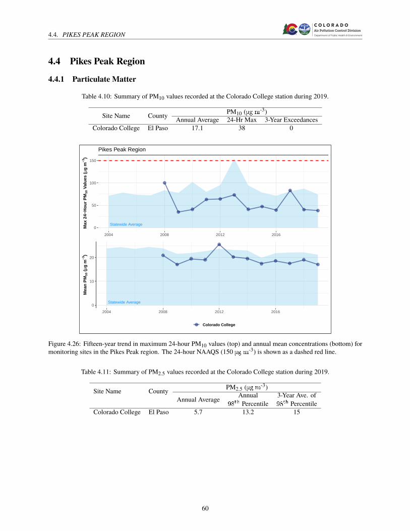
4.4. PIKES PEAK REGION

4.4 Pikes Peak Region


Table 4.10: Summary of PM10 values recorded at the Colorado College station during 2019.


Colorado College El Paso 17.1 38 0

Statewide Average0

50

100

150

2004 2008 2012 2016

Max

24−

Hou

r P

M10

Val

ues

(µg

m−3

)

Pikes Peak Region

Statewide Average0

10

20

2004 2008 2012 2016

Mea

n P

M10

(µg

m−3

)

Colorado College

Figure 4.26: Fifteen-year trend in maximum 24-hour PM10 values (top) and annual mean concentrations (bottom) formonitoring sites in the Pikes Peak region. The 24-hour NAAQS (150 μg m-3) is shown as a dashed red line.

Table 4.11: Summary of PM2.5 values recorded at the Colorado College station during 2019.




Colorado College El Paso 5.7 13.2 15

60


Statewide Average0

10

20

30

2004 2008 2012 2016

98th

Per

cent

ile P

M2.

5 V

alue

s (µ

g m

−3)

Pikes Peak Region


2.5

5.0

7.5

10.0

12.5

2004 2008 2012 2016

Ann

ual M

ean

PM

2.5

(µg

m−3

)

Colorado College

Figure 4.27: Fifteen-year trend in 24-hour PM2.5 annual 98th percentile values (top) and annual mean concentrations(bottom) for monitoring sites in the Pikes Peak region. The 24-hour and annual mean NAAQS (35 μg m-3 and 12 μgm-3, respectively) are shown as dashed red lines.

61


4.4.2 Carbon Monoxide

Table 4.12: Summary of CO values recorded at the Highway 24 (Colorado Springs) station during 2019.




Highway 24 El Paso 2.7 2.6 1.7 1.6

Statewide Average0

10

20

30

2004 2008 2012 2016

Max

1−H

our

CO

Val

ues

(ppm

)

Pikes Peak Region


2.5

5.0

7.5

2004 2008 2012 2016

Max

8−H

our

CO

Val

ues

(ppm

)


0.2

0.4

0.6

0.8

2004 2008 2012 2016

Mea

n C

O (

ppm

)

Highway 24

Figure 4.28: Fifteen-year trend in annual maximum one-hour (top) and eight-hour (center) CO values and annual meaneight-hour CO concentrations (bottom) for monitoring sites in the Pikes Peak region. The one-hour and eight-hourNAAQS (35 ppm and 9 ppm, respectively) are shown as dashed red lines.

62


4.4.3 Ozone

Table 4.13: Summary of O3 values recorded at monitoring stations in the Pikes Peak region during 2019.

Site Name CountyOzone 8-HourAverage (ppm)

1st Max. 4th Max. 3-Year Ave. of4th Max.

U.S. Air Force Academy El Paso 69 65 69Manitou Springs El Paso 70 64 68

Statewide Average0

20

40

60

80

2004 2008 2012 2016

4th M

ax 8

−Hou

r O

3 V

alue

s (p

pb)

Pikes Peak Region

Statewide Average0

10

20

30

40

2004 2008 2012 2016Ann

ual M

ean

8−H

our

O3

Val

ues

(ppb

)

Colorado Springs Manitou Springs

Figure 4.29: Fifteen-year trend in ozone eight-hour NAAQS values (top) and annual mean eight-hour concentrations(bottom) for monitoring sites in the Pikes Peak region. The eight-hour NAAQS (70 ppb) is shown as a dashed red line.

63


4.4.4 Sulfur Dioxide

Table 4.14: Summary of SO2 values recorded at the Highway 24 monitoring site in Colorado Springs during 2019.

Site Name County SO2 (ppb)

Annual Mean 99th

Percentile3-Year Ave. of99th Percentile

Highway 24 El Paso 0.92 9.6 13

Statewide Average0

20

40

60

2004 2008 2012 2016

99th

Per

cent

ile S

O2

Val

ues

(ppb

)

Pikes Peak Region

Statewide Average0

1

2

3

2004 2008 2012 2016

Ann

ual M

ean

SO

2 (p

pb)

Highway 24

Figure 4.30: Fifteen-year trend in sulfur dioxide one-hour NAAQS values (top) and annual mean one-hour concentra-tions (bottom) for monitoring sites in the Pikes Peak region. The one-hour NAAQS (75 ppb) is shown as a dashed redline.

64


4.4.5 MeteorologySee section 3.4 for more details on the wind rose plot below.

Highway 24


W

S

N

E

5%

10%

15%

20%

25%

30%

35%

mean = 2.1768calm = 0.1 %

(m s−1)

0 to 2

2 to 4

4 to 6

6 to 8

8 to 10

10 to 15.333

Figure 4.31: Wind rose from the Highway 24 meteorological station.

65

4.5. SOUTH CENTRAL REGION

4.5 South Central Region


Table 4.15: Summary of PM10 values recorded at the Pueblo monitoring station during 2019.


Pueblo Pueblo 17.9 89 2.2

Statewide Average0

50

100

150

2004 2008 2012 2016

Max

24−

Hou

r P

M10

Val

ues

(µg

m−3

)

South Central Region

Statewide Average0

5

10

15

20

25

2004 2008 2012 2016

Mea

n P

M10

(µg

m−3

)

Pueblo

Figure 4.32: Fifteen-year trend in maximum 24-hour PM10 values (top) and annual mean concentrations (bottom) formonitoring sites in the South Central region. The 24-hour NAAQS (150 μg m-3) is shown as a dashed red line.

Table 4.16: Summary of PM2.5 values recorded at the Pueblo monitoring station during 2019.




Pueblo Pueblo 5.5 8.4 13

66

4.5. SOUTH CENTRAL REGION

Statewide Average0

10

20

30

2004 2008 2012 2016

98th

Per

cent

ile P

M2.

5 V

alue

s (µ

g m

−3)

South Central Region


2.5

5.0

7.5

10.0

12.5

2004 2008 2012 2016

Ann

ual M

ean

PM

2.5

(µg

m−3

)

Pueblo

Figure 4.33: Fifteen-year trend in 24-hour PM2.5 annual 98th percentile values (top) and annual mean concentrations(bottom) for monitoring sites in the South Central region. The 24-hour and annual mean NAAQS (35 μg m-3 and 12μg m-3, respectively) are shown as dashed red lines.

67

4.6. SOUTHWEST REGION

4.6 Southwest Region


Table 4.17: Summary of PM10 values recorded at monitoring sites in the Southwest region during 2019.


Pagosa Springs School Archuleta 18.2 88 0

Statewide Average0

100

200

300

2004 2008 2012 2016

Max

24−

Hou

r P

M10

Val

ues

(µg

m−3

)

Southwestern Region

Statewide Average0

5

10

15

20

25

2004 2008 2012 2016

Mea

n P

M10

(µg

m−3

)

Pagosa Springs

Figure 4.34: Fifteen-year trend in maximum 24-hour PM10 values (top) and annual mean concentrations (bottom) formonitoring sites in the Southwest region. The 24-hour NAAQS (150 μg m-3) is shown as a dashed red line.

68

4.6. SOUTHWEST REGION

4.6.2 Ozone

Table 4.18: Summary of O3 values recorded at the monitoring station in the Southwest region during 2019.



Cortez - Health Dept. Montezuma 64 60 62

Statewide Average0

20

40

60

80

2004 2008 2012 2016

4th M

ax 8

−Hou

r O

3 V

alue

s (p

pb)

Southwestern Region

Statewide Average0

10

20

30

2004 2008 2012 2016Ann

ual M

ean

8−H

our

O3

Val

ues

(ppb

)

Cortez

Figure 4.35: Fifteen-year trend in ozone eight-hour NAAQS values (top) and annual mean eight-hour concentrations(bottom) for monitoring sites in the Southwest region. The eight-hour NAAQS (70 ppb) is shown as a dashed red line.

69

4.7. WESTERN SLOPE REGION

4.7 Western Slope Region


Table 4.19: Summary of PM10 values recorded at monitoring sites in the Western Slope region during 2019.


Grand Junction - Powell Bldg. Mesa 15.2 47 0Telluride San Miguel 14.0 61 0

Statewide Average0

100

200

300

2004 2008 2012 2016

Max

24−

Hou

r P

M10

Val

ues

(µg

m−3

)

Western Slope Region

Statewide Average0

10

20

30

2004 2008 2012 2016

Mea

n P

M10

(µg

m−3

)

Grand Junction − Powell Bldg. Telluride

Figure 4.36: Fifteen-year trend in maximum 24-hour PM10 values (top) and annual mean concentrations (bottom) formonitoring sites in the Western Slope region. The 24-hour NAAQS (150 μg m-3) is shown as a dashed red line.

70


Table 4.20: Summary of PM2.5 values recorded at the Grand Junction - Powell Bldg. monitoring site during 2019.




Grand Junction - Powell Bldg. Mesa 5.0 14.5 6

Statewide Average0

10

20

30

2004 2008 2012 2016

98th

Per

cent

ile P

M2.

5 V

alue

s (µ

g m

−3)



2.5

5.0

7.5

10.0

12.5

2004 2008 2012 2016

Ann

ual M

ean

PM

2.5

(µg

m−3

)

Grand Junction − Powell Bldg.

Figure 4.37: Fifteen-year trend in 24-hour PM2.5 annual 98th percentile values (top) and annual mean concentrations(bottom) for monitoring sites in the Western Slope region. The 24-hour and annual mean NAAQS (35 μg m-3 and 12μg m-3, respectively) are shown as dashed red lines.

71


4.7.2 Carbon MonoxideThe Grand Junction - Pitkin CO monitor was removed on 6/1/2019. Therefore, the data reported here is based on onlyfive months of monitoring.

Table 4.21: Summary of CO values recorded at the Grand Junction - Pitkin station during 2019.




Grand Junction - Pitkin Mesa 1.7 1.1 0.7 0.7

Statewide Average0

10

20

30

2004 2008 2012 2016

Max

1−H

our

CO

Val

ues

(ppm

)



2.5

5.0

7.5

2004 2008 2012 2016

Max

8−H

our

CO

Val

ues

(ppm

)


0.2

0.4

0.6

2004 2008 2012 2016

Mea

n C

O (

ppm

)

Grand Junction

Figure 4.38: Fifteen-year trend in annual maximum one-hour (top) and eight-hour (center) CO values and annual meaneight-hour CO concentrations (bottom) for monitoring sites in the Western Slope region. The one-hour and eight-hourNAAQS (35 ppm and 9 ppm, respectively) are shown as dashed red lines.

72


4.7.3 Ozone

Table 4.22: Summary of O3 values recorded at monitoring stations in the Western Slope region during 2019.



Rifle - Health Dept. Garfield 62 57 60Palisade Water Treatment Mesa 65 63 65

Statewide Average0

20

40

60

80

2004 2008 2012 2016

4th M

ax 8

−Hou

r O

3 V

alue

s (p

pb)


Statewide Average0

10

20

30

40

2004 2008 2012 2016Ann

ual M

ean

8−H

our

O3

Val

ues

(ppb

)

Palisade Rifle

Figure 4.39: Fifteen-year trend in ozone eight-hour NAAQS values (top) and annual mean eight-hour concentrations(bottom) for monitoring sites in the Western Slope region. The eight-hour NAAQS (70 ppb) is shown as a dashed redline.

73


4.7.4 MeteorologySee section 3.4 for more details on the wind rose plots below.

Palisade Water Treatment


W

S

N

E

10%

20%

30%

40%

50%

60%

mean = 1.6029

calm = 0 %

(m s−1)

0 to 2

2 to 4

4 to 6

6 to 8

8 to 10

Grand Junction − Pitkin


W

S

N

E

5%

10%

15%

20%

25%

30%

mean = 2.0014

calm = 0 %

(m s−1)

0 to 2

2 to 4

4 to 6

6 to 8

8 to 10

10 to 13.858

Figure 4.40: Wind roses for sites in the Western Slope Region during 2019.

74

5

Seasonal Variability in Air Quality

Data has been presented in this report to give an overall picture of the progress of air quality through the years and tocompare measured concentrations against the NAAQS. However, APCD collects data as hourly averages (which arethemselves the result of even more brief intervals being averaged together) for select criteria pollutants at each site. Inthis section, monthly averages will be presented for each site.

In some sense, there is little interpretation to be done concerning the air quality information presented in this section.It is not intended to compare Colorado’s air quality against the standards, other states, or past air quality. This sectionis only to suggest a more detailed picture of the air quality in our state throughout the year.

In all of the graphs in this section, the range is illustrated as blue shading, where the lower and upper limits aredefined as the minimum and maximum monthly averages, respectively. This is the range for the entire state. The sitesare not grouped by monitoring region in this section, rather they are presented in order of their Air Quality Site ID,which is an EPA designated code derived from the state and county where the site is located, along with a unique sitenumber. Each graph has been limited in the number of sites it presents for clarity sake, but for each pollutant set, theminimum and maximum state-wide range is the same. Data in the graphs below may include exceptional events (seesubsubsection 2.2.5.4).

5.1 Carbon MonoxideCO is normally higher in the winter months and lower in the summer, for reasons previously discussed (see subsec-tion 2.2.1).

75

5.1. CARBON MONOXIDE

0.2

0.4

0.6

Jan Feb Mar Apr May Jun Jul Aug Sep Oct Nov Dec

Mon

thly

Mea

n C

arbo

n M

onox

ide

(ppm

)

Welby CAMP I−25: Denver La Casa Highway 24

Figure 5.1: Monthly mean carbon monoxide concentrations. The blue shaded region shows the statewide range ofmonthly mean values.

0.2

0.4

0.6


Mon

thly

Mea

n C

arbo

n M

onox

ide

(ppm

)

Fort Collins Grand Junction Greeley

Figure 5.2: Monthly mean carbon monoxide concentrations. The blue shaded region shows the statewide range ofmonthly mean values.

76

5.2. SULFUR DIOXIDE

5.2 Sulfur DioxideSulfur dioxide was measured at four stations during 2019 by APCD in Colorado: Welby, La Casa, CAMP, andHighway 24 (Colorado Springs). Sulfur dioxide generally follows the same pattern as that for CO, typically beinglower in concentration during the warmer months and higher in concentration during the colder months.

0.6

0.9

1.2


Mon

thly

Mea

n S

ulfu

r D

ioxi

de (

ppb)

Welby CAMP La Casa Highway 24

Figure 5.3: Monthly mean sulfur dioxide concentrations. The blue shaded region shows the statewide range of monthlymean values.

77

5.3. OZONE

5.3 OzoneOzone follows an opposite seasonal pattern relative to CO. The summer months see high ozone and the winterexperiences lower levels, in part because of seasonal variations in day length and the angle of the sun relative to theground. Remember that ozone may be indicative of ground-level smog or the “Denver Brown Cloud.” Generallyspeaking, sites in the Northern Front Range counties experienced higher concentrations of ozone than other areas(especially sites directly west of, and at higher elevation than, metro Denver), though sites outside the Front Rangeoccasionally had the highest averages. Note that data for the non-regulatory Mines Peak O3 site is shown below forinformational purposes.

10

20

30

40

50


Mon

thly

Mea

n O

zone

(pp

b)

Welby

Aurora − East

Highland Res.

Boulder Res.

Mines Peak

CAMP

Figure 5.4: Monthly mean ozone concentrations. The blue shaded region shows the statewide range of monthly meanvalues.

10

20

30

40

50


Mon

thly

Mea

n O

zone

(pp

b)

La Casa

Chatfield

Colorado Springs

Manitou Springs

Rifle

Black Hawk


78

5.3. OZONE

10

20

30

40

50


Mon

thly

Mea

n O

zone

(pp

b)

Aspen Park

NREL

Rocky Flats

Welch

Fort Collins

Fort Collins − West


10

20

30

40

50


Mon

thly

Mea

n O

zone

(pp

b)

Palisade Cortez Greeley


79

5.4. NITROGEN DIOXIDE

5.4 Nitrogen DioxideNitrogen dioxide was measured at six stations during 2019 by APCD in Colorado: Welby, Camp, La Casa, I-25Globeville, I-25 Denver, and Rocky Flats. Nitrogen dioxide generally follows the same pattern as that for CO, typicallybeing lower in concentration during the warmer months and higher in concentration during the colder months. NO2concentrations at sites in fairly close proximity appear to track well with one another.

10

20

30


Mon

thly

Mea

n N

itrog

en D

ioxi

de (

ppb)

Welby

CAMP

I−25: Denver

I−25: Globeville

La Casa

Rocky Flats

Figure 5.8: Monthly mean nitrogen dioxide concentrations. The blue shaded region shows the statewide range ofmonthly mean values.

80

5.5. PM10

5.5 PM10PM10 concentrations can be elevated for a variety of reasons, including both anthropogenic and natural occurrences.Higher PM10 concentrations might be expected during dry months and or droughts, since the soil has a chance todry out and be entrained by the winds. This is reflected somewhat in the range of PM10 concentrations found in thefollowing graphs, but the peaks in concentrations are often due to single-point high-concentration events, typicallyassociated with high winds and blowing dust. The data below contains exceptional events. See subsubsection 2.2.5.4for an explanation of exceptional events. Many of these exceptional events will be analyzed and documented as naturalevents and be demonstrated as beyond reasonable control and or not preventable. The documentation package is thensent to the EPA for concurrence. If the EPA concurs with the APCD‘s analysis, then the exceedance or high PM10reading will be removed from regulatory consideration and will not be used in NAAQS calculations.

10

20

30

40

50


Mon

thly

Mea

n P

M10

(µg

m−3

)

TCH

Welby

Pagosa Springs

Boulder − CC

Longmont

CAMP

Figure 5.9: Monthly mean PM10 concentrations. The blue shaded region shows the statewide range of monthly meanvalues.

10

20

30

40

50


Mon

thly

Mea

n P

M10

(µg

m−3

)

La Casa

Colorado College

Cañon City

Grand Junction − Powell Bldg.

Aspen

Lamar


81

5.5. PM10

10

20

30

40

50


Mon

thly

Mea

n P

M10

(µg

m−3

)

Pueblo Steamboat Springs Telluride


82

5.6. PM2.5

5.6 PM2.5PM2.5 concentrations are generally stable throughout much of the year, reaching maximum values during the wintermonths. Relatively similar values are measured at sites throughout the state. The graphs here may include exceptionalevent data.

4

8

12

16


Mon

thly

Mea

n P

M2.

5 (µ

g m

−3)

TCH ACC Boulder − CC Longmont CAMP

Figure 5.12: Monthly mean PM2.5 concentrations. The blue shaded region shows the statewide range of monthly meanvalues.

4

8

12

16


Mon

thly

Mea

n P

M2.

5 (µ

g m

−3)

I−25: Denver

I−25: Globeville

La Casa

NJH

Chatfield

Colorado College


83

5.6. PM2.5

4

8

12

16


Mon

thly

Mea

n P

M2.

5 (µ

g m

−3)

Fort Collins − CSU Grand Junction − Powell Bldg. Pueblo Greeley − Hospital Platteville


84

6

Data Quality Assurance / Quality Control

This section describes the APCD Technical Services Program’s success in meeting its data quality objectives forambient air pollution monitoring data of criteria pollutants. This section has been prepared in accordance with 40CFR Part 58 requirements. The statistical methodology used in this assessment is described in detail in the document"Guideline on the Meaning and Use of Precision and Accuracy Data Required by 40 CFR Part 58 Appendix A."

Other quality objectives were assessed via laboratory and site system audits. The results of these audits indicatecompliance with APCD’s standard operating procedures and EPA acceptance criteria. Copies of APCD laboratoryaudits may be obtained from the Quality Assurance Unit of the APCD.

Other audits were performed and can be made available for review, including National Air Toxics Trends Station(NATTS) audits, Speciation TrendNetwork (STN) audits, and audits conductedwithin Colorado by other organizations.These results are not included in this report because other agencies perform the data assessments for these audits.CDPHE meteorological network audits are not included in this report, as meteorological data is not considered apriority pollutant and so a statistical assessment of this data is not provided.

6.1 Data QualityIn order to provide decision makers with data of adequate quality, the CDPHE uses the Data Quality Objectives (DQO)process to develop performance and acceptance criteria (or data quality objectives) that specify tolerable levels ofpotential decision errors that will be used as the basis for establishing the quality and quantity of data needed tosupport decisions. Quality objectives for measurement data are designed to ensure that the data end user’s DQOsare met. Measurement quality objectives include quantitative objectives, such as representativeness, completeness,accuracy, precision, and detection level, as well as qualitative objectives, such as site placement, operator training, andsample handling techniques. There are some data quality indicators underlying the DQOs that relate directly to themeasurement system being used to collect ambient air measurements. These data quality indicators include precision,bias, completeness, and sampling frequency. These variables need to be maintained within certain acceptable rangesso that end data users can make decisions with specified levels of confidence.

85

6.2. QUALITY ASSURANCE PROCEDURES

6.2 Quality Assurance ProceduresQuality assurance is a general term for the procedures used to ensure that a particular measurement meets the qualityrequirements for its intended use. In addition to performing tests to determine bias and precision, additional qualityindicators (such as sensitivity, representativeness, completeness, timeliness, documentation quality, and sample custodycontrol) are also evaluated. Quality assurance procedures fall under two categories:

• Quality Control (QC): procedures built into the daily sampling and analysis methodologies to ensure data quality,and

• Quality Assessment (QA): periodic independent evaluations of data quality.

Some ambient air monitoring is performed by automated equipment located at field sites, while other measurements aremade by taking samples from the field to the laboratory for analysis. For this reason, we will divide quality assuranceprocedures into two parts: field and laboratory quality assurance.

6.2.1 Field Quality AssuranceQuality assurance is a general term for the procedures used to ensure that a particular measurement meets the qualityrequirements for its intended use. Quality control of continuous analyzers consists of precision checks or flowverifications. The overall precision of filter-based sampling methods is measured using collocated samplers. Qualityassurance is evaluated by periodic performance and system audits.

Automated analyzers (except O3) are calibrated by challenging the instrument’s response to a known concentration ofEPA protocol gas delivered through a dilution system. The analyzer is then adjusted to produce the correct response.O3 analyzers are calibrated by challenging the analyzer’s response with O3 produced by an independently certifiedNIST-traceable ozone generator. The site’s analyzer is then adjusted to produce the same measured concentration asthe traceable analyzer. Manual samplers are calibrated by comparing their volumetric flow rate at one or more levels tothe flow measured by a flow transfer standard. Calibrations are performed when an instrument is first installed and atassigned intervals thereafter depending on the analyzer type. Calibrations are also performed after instrument repairsor when quality control charts indicate a drift in response to quality control checks.

Precision is a measure of the variability of an instrument or the variability of the testing source. The precision ofcontinuous gaseous analyzers are evaluated by comparing a sample of a known concentration against the instrument’sresponse. The precision of filter-based particulate samplers is determined by collocated sampling (i.e., the simultaneousoperation of two identical samplers placed side by side). The difference in the results of the two samplers is usedto estimate the precision of the entire measurement process (i.e., both field and laboratory precision). Precision ofmanual particulate samplers is assessed by regular periodic flow checks. Precision of continuous particulate samplersis assessed through the comparison of the ambient data to the FRM data and by regular periodic flow checks. Manualsamplers are calibrated by comparing their volumetric flow rate at one or more levels to the flow measured by a flowtransfer standard. Calibrations are performed when an instrument is first installed and at assigned intervals thereafterdepending on the analyzer type. Calibrations are also performed after instrument repairs or when quality control chartsindicate a drift in response to quality control checks.

The bias of automated methods is assessed through field performance evaluations (also called accuracy audits) andthrough site precision checks. Performance audits are conducted by challenging the instrument with a gas of knownNIST-traceable concentration. Bias is evaluated by comparing the measured response to the known value. Typically,performance evaluations are performed biannually using samples of several different concentrations.

System audits indicate how well a sampling site and site operator conforms to the standard operating procedures aswell as how well the site is located with respect to its mission (e.g., urban or rural sampling, SLAMS or specialpurpose sampling site, etc.). Some areas reviewed include: site location (possible obstruction, presence of nearbypollutant sources), site security, site characteristics (urban versus suburban or rural), sitemaintenance, physical facilities(maintenance, type and operational quality of equipment, buildings, etc.), record-keeping, sample handling, storage,and transport.

86

6.3. GASEOUS CRITERIA POLLUTANTS

6.2.2 Laboratory Quality ControlLaboratory quality control includes calibration of analytical instrumentation, analysis of blank samples to checkfor contamination, analysis of spikes to evaluate interferences and target analyte matrix recovery, and analysis ofduplicate samples to evaluate precision. Quality assurance is accomplished through laboratory performance andsystem audits.

Laboratory analytical instruments are calibrated by comparing the instrument’s response with standards of a knownconcentration level. The differences between the measured and known concentrations are then used to adjust theinstrument to produce the correct response.

A blank sample is one that has intentionally not been exposed to the pollutant of interest. Analysis of blank samplesreveals possible contamination in the laboratory, during field handling, or during transportation.

Duplicate analyses of the same sample are performed to monitor the precision of the analytical method.

A regular sample is spiked with a known concentration to determine if the sample matrix is interfering with detectioncapabilities of the instrumentation. Regular performance audits are conducted by having the laboratory analyze sampleswhose physical or chemical properties have been certified by an external laboratory or standards organization. Thedifference between the laboratory’s reported value and the certified value is used to evaluate the analytical method’saccuracy.

System audits indicate how well the laboratory conforms to its standard operating procedures. System audits involvesending a QA Auditor to the laboratory to review compliance with standard operating conditions. Areas examinedinclude: record keeping, sample custody, equipment maintenance, personnel training and qualifications, and a generalreview of facilities and equipment.

6.3 Gaseous Criteria Pollutants

6.3.1 Quality Objectives for Measurement DataData Quality Objectives for the APCD’s ambient air monitoring program for gaseous criteria pollutants are shown inTable 6.1.

Table 6.1: Data quality objectives for gaseous criteria pollutants.

Data Quality Indicator APCD Goal EPA RequirementPrecision for O3 7% 7%

Precision for CO, SO2, NO2 10% 10%Precision Completeness 90% 75%

Bias for O3 7% 7%Bias for CO, SO2, NO2 10% 10%

Accuracy for O3 10% 10%Accuracy Audits Completeness 2 audits per analyzer per year 25% of analyzers quarterly

90% Probability Intervals Meet EPA requirement 95% of audit valuesNPAP TTP Audits for O3 Meet EPA requirement 10%

NPAP TTP Audits for for CO, SO2, NO2 Meet EPA requirement 15%Overall Data Completeness 90% 75%

6.3.2 Gaseous Data Quality Assessment6.3.2.1 Summary

Assessment of the data forAPCDgaseous criteria pollutants showed that themajority of gaseous analyzersmetminimumEPA criteria and APCD goals for precision, bias, accuracy, national performance evaluations, and completeness in2019. O3 data for the U.S. Air Force Academy site was invalidated from 12/4/2018 to 5/17/2019 due to sampleline configuration issues, which resulted in this site failing to meet goals for both data and precision completeness.The I-25 Globeville site failed to meet completeness requirements for precision due to inconsistencies in the timing

87


Table 6.2: Summary of precision, accuracy, bias, and completeness for site-level gaseous monitoring data.

Site Parameter PrecisionCount

PrecisionComplete (%)

CV(%)

Bias(%)

Prob. Limits DataComplete (%)Lower Upper

Welby CO 22 85 2.1 +/-1.68 -3.3 3.37 94CAMP CO 23 88 2.65 +/-2.42 -3.23 5.22 97La Casa CO 22 85 3.68 +/-3.02 -5.61 6.12 96I-25: Denver CO 22 85 2.88 +4.44 -0.99 8.16 98Highway 24 CO 21 81 3.08 +/-2.54 -4.69 5.11 96Fort Collins - Mason CO 21 81 1.26 +1.24 -1.22 2.77 95Greeley - Weld County Tower CO 23 88 2.75 +2.38 -3.15 5.59 97Welby SO2 22 85 3.99 +/-3.19 -5.54 7.15 93CAMP SO2 24 92 4.84 +4.7 -5.45 9.93 98La Casa SO2 22 85 2.88 -3.96 -7.6 1.57 91Highway 24 SO2 22 85 3.55 +/-2.93 -5.75 5.55 90Welby NO2 21 81 2.08 -3.64 -6.35 0.24 90CAMP NO2 21 81 2.44 +4.05 -0.51 7.22 94La Casa NO2 21 81 3.34 +/-2.66 -4.56 5.9 85I-25: Denver NO2 21 81 3.27 +/-2.67 -4.62 5.73 93I-25: Globeville NO2 15 58 3.48 -4.18 -8.26 2.32 90Rocky Flats - N. NO2 23 100 2.34 +/-1.93 -4.19 3.16 94Mines Peak O3 18 69 2.62 +3.0 -1.99 6.24 79Welby O3 23 88 3.16 +/-2.89 -6.34 3.7 93Highland Reservoir O3 21 81 2.5 +2.24 -3.01 4.94 97Aurora - East O3 21 81 2.62 +/-2.8 -5.86 2.48 96Boulder Reservoir O3 23 88 1.56 +/-1.24 -2.41 2.55 99CAMP O3 22 85 2.97 +/-2.5 -5.67 3.79 99La Casa O3 22 85 2.58 +/-2.11 -4.59 3.61 92Chatfield State Park O3 22 85 1.92 +/-1.52 -3.1 2.99 95U.S. Air Force Academy (USAFA) O3 14 54 1.9 +/-1.59 -3.26 2.41 62Manitou Springs O3 22 85 1.92 +3.02 -0.58 5.51 99Black Hawk O3 9 69 1.85 -3.49 -5.31 -0.26 77Welch O3 23 88 2.63 +/-2.54 -5.61 2.77 97Rocky Flats - N. O3 23 88 1.61 -2.68 -4.76 0.36 98NREL O3 22 85 2.05 +1.95 -2.26 4.26 96Aspen Park O3 15 83 1.93 -2.01 -4.26 1.62 97Fort Collins - West O3 23 88 1.41 +1.43 -1.33 3.15 99Fort Collins - Mason O3 22 85 2.26 +2.44 -2.05 5.16 94Greeley - Weld County Tower O3 23 88 2.8 +/-2.33 -3.9 5.0 97

of the precision checks and the AQS database procedure for calculating completeness. These inconsistencies resultin artificially low precision completeness values at most sites, a problem that the APCD is working to address in2020.

6.3.2.2 Coefficient of Variation (CV)

At least once every two weeks, precision is determined by sampling a gas of known concentration for every gaseousanalyzer. Table 6.2 summarizes the number of precision checks that were performed (precision count) by site as well asthe percent completeness of those precision checks. Table 6.2 also summarizes the statistical data quality assessmentof these precision checks for all gaseous criteria pollutants. The coefficient of variation (CV) for the precision checks issummarized annually by site. The equations used to calculate precision, bias, and upper and lower probability limits forthe 90% probability intervals using the bi-weekly precision checks are described in detail in the document "Guidelineon the Meaning and Use of Precision and Accuracy Data Required by 40 CFR Part 58 Appendix A."

6.3.2.3 Bias

For gaseous pollutants the bias is also calculated using the bi-weekly precision checks. Bias is summarized in Table 6.2by the same groupings as CV. Additionally a plus or minus bias is assigned to the annual site and organization groupinglevels based on an evaluation of where the 25th and 75th percentiles of percent differences for the precision data fell.If both percentiles fell below zero then the bias was assigned a minus sign, and if both percentiles fell above zero, thenthe bias was assigned a plus sign. If one bias was positive and one bias was negative (i.e. straddling zero), no sign wasassociated with the bias. Organizationally, CO showed a non-signed bias of 1.93% in 2019. SO2 showed a non-signed

88


bias of 3.41%. O3 showed a non-signed bias of 1.93% for 2019. There was no sign associated with the calculated bias(2.81%) for the NO2 precision checks for the organization as a whole in 2019.

6.3.2.4 Performance Evaluation (Accuracy Audits)

Audits were performed at least twice on every gaseous analyzer within the APCD network during the 2019 calendaryear. The primary goal of these audits is to evaluate the analyzer performance and calibration. Other factors are alsonoted during these audits such as operator performance, station operational criteria, record keeping, site upkeep issues,and general safety problems.

6.3.2.5 Probability Intervals (Upper and Lower Probability Limits)

Probability intervals (upper and lower probability limits) are calculated per 40 CFR 58 Appendix A section 4, by usingthe percent differences retrieved from station precision checks. The EPA has established that 95% of the independentaudit points taken for a given year should fall within this calculated probability interval to validate the bias calculatedfrom the precision checks. The percent differences between the audit concentrations and the indicated concentrationstaken in 2019 for CO were compared to the probability intervals. Out of the 57 audit concentration points takenfor CO in 2019, 49% fell between the probability intervals for the organization. There were 137 audit concentrationpoints taken during 2019 for the APCD’s O3 network. Of those 137 ozone audit points, 24 fell outside the probabilityintervals. This means that 82% of the audit points for O3 fell between the probability intervals in 2019. Out of the120 audit points taken in 2019 for NO2, 73% fell between the probability limits. Out of the 33 audit points taken forSO2 in 2019, 79% fell between the probability intervals. Therefore, all four gaseous criteria pollutants do not meet therequirement that specifies that ninety-five percent of the individual percent differences (all audit concentration levels)for the performance evaluations should be captured within the probability intervals for the primary quality assuranceorganization (40CFR 58 Appendix A section 4.1.5).

APCD believes the reason it did not meet the above requirement in 2019 is due to the fact that the probability intervalsare calculated based on precision checks that are closer to the middle of the calibration scale, which give small percentdifferences and tight probability intervals. A newer requirement in the CFR is pushing APCD to audit in the lowerportion of the site instrumentation’s calibration scale, due to the fact that this is where 80% of the ambient data isbeing captured. By auditing in the low end of the calibration scale, APCD is seeing higher percent differences betweenthe audit concentration and the instrument response. APCD believes this is due in part to the low audit concentrationdifferences producing large percent differences and partly because the instruments are calibrated on a higher scale thanwhere the audits are being conducted. The instruments are being calibrated at a higher scale than where 80% of theambient data falls due to the relatively small number of episodes that do produce high ambient concentrations whichhave an effect on public health. Recently, APCD has begun to lower the calibration range on most pollutants and lowerthe precision values at most of its sites. This will hopefully help to rectify this problem but still allow APCD to capturethe higher concentration pollution episodes within the instrument’s calibration range.

6.3.2.6 Completeness

Data completeness for the year is shown by site in Table 6.2. Precision completeness is shown as the number ofprecision checks that were performed and submitted to AQS for the year. Precision completeness is evaluated againstthe number of checks that should have been performed at each site during the year. Completeness for accuracy auditsin 2019 met or exceeded APCD DQO goals for every gaseous analyzer, with a minimum of two audits performed onevery analyzer.

Table 6.2 summarizes the statistical evaluations for all gaseous precision, accuracy, bias, and completeness data. Thebasis for these calculations can be found in 40 CFR 58 Appendix A section 4.1.

89

6.4. PARTICULATE DATA QUALITY ASSESSMENT

6.4 Particulate Data Quality Assessment

6.4.1 SummaryAssessment of the data quality for APCD particulate criteria pollutants showed that most samplers met minimum EPAcriteria and most monitoring sites met APCD goals for accuracy, precision, completeness, and bias.

6.4.2 PrecisionThe CV for filter-based particulate monitoring is determined from the collocated precision data collected (i.e., twoidentical samplers operated in an identical manner). Due to the anticipated poor precision for very low levels ofpollutants, only collocated measurements at or above a minimum level (greater than or equal 15 μg m-3 for PM10, 20μg m-3 for Total Suspended Particulate or TSP, and 3 μg m-3 for PM2.5) would be called valid pairs and are used toevaluate precision. The calculations for the statistical presentations in Table 6.3 are found in 40 CFR 58 Appendix Asection 4.2.

The CV for continuous based particulate monitoring is determined by monthly flow verifications (precision checks)performed on the continuous particulate monitors. The calculations for the statistical presentations in Table 6.3 are thesame calculations that were performed on the precision data for gaseous analyzers.

6.4.3 BiasResults of the annual flow rate audits conducted by APCD personnel are shown in Table 6.3 below. There is norequirement for bias on the High-Vol filter-based particulate monitoring, since the precision is based on collocatedsampling. For the filter-based particulate monitoring, Table 6.3 summarizes bias based on the audits that wereperformed during the year, since APCD performs particulate audits four times more frequently than the EPA requires.These additional audits are conducted to compensate for the lack of a flow verification precision check program inplace for the High-Vol samplers. The bias for the continuous particulate monitoring was calculated on the monthlyflow verification precision checks with the same calculations that were used to determine the gaseous bias.

6.4.4 Performance Evaluation (Accuracy Audits)Audits were performed at least quarterly on every particulate sampler within the APCD network during the 2019calendar year. The primary goal of these audits is to evaluate the analyzer performance and calibration. Other factorsare also noted during these audits such as operator performance, station operational criteria, record keeping, site upkeepissues, and general safety problems.

6.4.5 CompletenessData completeness for the year is shown by site in Table 6.3. Precision completeness is based on the number of monthlyflow verifications that were performed. Precision completeness is evaluated against the number of checks that shouldhave been performed at each site during the year. Completeness for accuracy audits met or exceeded all APCD DQOgoals for every particulate analyzer, with a minimum of two audits performed on every analyzer per year.

90

6.4. PARTICULATE DATA QUALITY ASSESSMENT

6.4.6 ResultsTable 6.3 below summarizes statistical evaluations for all filter-based particulate precision, accuracy, bias, and com-pleteness data. The values were calculated as described in 40 CFR 58 Appendix A section 4.2.

Table 6.3: Summary of precision, accuracy, bias, and completeness for filter-based particulate monitoring data.

Site Parameter VerificationCount

VerificationComplete (%)

Bias(%)

Mean %Difference

Std. Dev. %Difference

Tri County Health (TCH) PM10 12 100 -0.72 -0.27 0.63Welby PM10 2 50 +/-5.08 0.62 1.69Welby PM10 30 100 -1.38 -0.85 1.07Pagosa Springs School PM10 9 100 +/-2.92 -0.86 2.43Longmont - Municipal Bldg. PM10 1 25 -0.6 -0.6 -Longmont - Municipal Bldg. PM10 1 25 -0.28 -0.28 -Boulder Chamber of Commerce (CC) PM10 2 50 +/-2.91 -0.38 0.68CAMP PM10 1 25 -1.18 -1.18 -CAMP PM10 1 25 -2.57 -2.57 -La Casa PM10 12 100 +1.1 0.77 0.61La Casa PM10 12 100 +1.07 0.75 0.6Colorado College PM10 26 100 +/-0.95 0.4 0.85Cañon City - City Hall PM10 2 50 +8.52 1.87 1.49Grand Junction - Powell Bldg. PM10 19 100 +/-1.17 0.5 1.02Grand Junction - Powell Bldg. PM10 17 100 +/-1.51 -0.14 1.45Aspen PM10 2 50 +2.35 0.9 0.32Lamar - Municipal Bldg. PM10 10 100 +/-2.26 -0.43 1.98Pueblo - Fountain School PM10 2 50 +/-3.51 -0.28 2.45Steamboat Springs PM10 12 100 +/-2.1 -0.65 1.82Telluride PM10 3 75 +/-2.91 -0.09 2.03Tri County Health (TCH) PM2.5 10 83 -1.12 -0.39 0.93Tri County Health (TCH) PM2.5 21 100 +/-3.49 -0.43 3.55Arapaho Community College (ACC) PM2.5 13 100 +/-1.18 0.66 0.87Longmont - Municipal Bldg. PM2.5 17 100 -1.26 -0.77 0.92Longmont - Municipal Bldg. PM2.5 15 100 +/-2.31 -0.66 2.09Boulder Chamber of Commerce (CC) PM2.5 22 100 -1.61 -1.3 0.81CAMP PM2.5 22 100 +/-0.35 0.03 0.34CAMP PM2.5 22 100 +/-0.45 0.21 0.39CAMP PM2.5 23 100 +/-2.49 0.46 2.48National Jewish Health (NJH) PM2.5 21 100 +1.6 1.02 1.16La Casa PM2.5 13 100 +1.75 1.44 0.64La Casa PM2.5 19 100 +/-0.7 0.36 0.56I-25: Denver PM2.5 17 100 +1.36 1.11 0.59I-25: Denver PM2.5 22 100 +/-2.24 0.24 2.27I-25: Globeville PM2.5 21 100 +/-3.25 -1.25 2.94Chatfield State Park PM2.5 14 100 +/-0.39 -0.1 0.35Chatfield State Park PM2.5 24 100 +/-2.01 0.94 1.71Colorado College PM2.5 28 100 +/-3.33 1.15 3.16Fort Collins - CSU PM2.5 29 100 +/-3.04 -0.02 3.17Grand Junction - Powell Bldg. PM2.5 21 100 +/-3.75 -2.0 3.12Pueblo - Fountain School PM2.5 26 100 +/-0.73 0.01 0.8Greeley - Hospital PM2.5 27 100 +/-2.99 -0.58 3.03Platteville - Middle School PM2.5 24 100 +/-0.54 0.35 0.43

91

6.5. EPA DATA QUALITY ASSESSMENT

Table 6.4: Collocated QC check statistics for particulate monitoring data. Sites with asterisks indicate a comparison ofa filter-based method with a 24-hour average value derived from a continuous monitor. Other sites involve a comparisonof collocated filter-based monitors.

Site Parameter Total Valid Pairs CVCAMP PM10 57 6.09La Casa PM10 57 4.61Longmont PM10 57 10.01GJ - Powell Bldg. PM10 59 9.04Tri County Health∗ PM2.5 53 17.24CAMP PM2.5 49 8.33La Casa∗ PM2.5 104 11.95I-25 Denver∗ PM2.5 58 19.44

6.5 EPA Data Quality Assessment

6.5.1 PEP / NPAP AuditsThe performance audits conducted during 2019 are summarized in Table 6.5 and Table 6.6.

Table 6.5: PM2.5 PEP results.

Audit Date Site PEP Result(μg m-3)

Site Result(μg m-3)

PercentDifference

2019/02/26 Chatfield State Park 21.4 21.1 1.4%2019/05/15 Grand Junction - Powell Bldg. 4.9 14.0 96.3%2019/06/11 I-25 Denver 6.9 8.0 14.7%2019/09/18 Arapaho Community College (ACC) 6.5 5.2 22.2%2019/09/18 Chatfield State Park 5.6 5.3 5.5%2019/11/05 Grand Junction - Powell Bldg. 6.2 23.0 115.1%2019/11/11 I-25 Denver 8.1 6.8 17.5%

Table 6.6: NPAP results for gaseous audits.

Audit Date Site Parameter Percent DifferencesL2 L3 L4 L5 L6 L7

2019/05/14 NREL O3 -1.9% 2.9% 1.8% 1.6%2019/05/15 U.S. Air Force Academy (USAFA) O3 9.6% 10.7% 11.2%2019/05/15 Manitou Springs O3 2.3% 2.2% 1.9% 1.2%2019/05/16 Highway 24 CO -20.2% -1.1% -4.3% -2.9%2019/05/16 Highway 24 SO2 -2.9% 2.0% 2.2% 2.0%2019/07/31 Cortez - Health Dept. O3 7.0% 0.0% -0.1%

92

APPENDIX A: MONITORING SITE DESCRIPTIONS

This appendix provides detailed information for all monitoring sites considered in this Data Report. Table A-1 summarizes the locations and monitoring parameters of each site currently in operation, by county, alphabetically. The shaded lines in the table list the site AQS identification numbers, address, site start-up date, elevation, and longitude and latitude coordinates. Beneath each site description the table lists each monitoring parameter in operation at that site, the orientation and spatial scale, which national monitoring network it belongs to, the type of monitor in use, and the sampling frequency. The parameter date is the date when valid data were first collected.

The following abbreviations are used in Table A-1 below, with orientation (Orient) referring to the monitoring objective and scale referring to the size of the area that concentrations from the monitor represent.

Orientation Scale (Area Represented)1 P.O. - Population oriented Micro - Micro-scale (several m – 100 m) Back - Background orientation Middle - Middle Scale (100 – 500 m) SPM - Special Purpose Monitor Neigh - Neighborhood Scale (0.5 – 4 km) H.C. - Highest Concentration Urban - Urban Scale (4 – 50 km) POC - Parameter Occurrence Code Region - Regional Scale (50 – hundreds of km) SLAMS - State or Local Air Monitoring Stations

Table A-1. Monitoring Locations and Parameters Monitored

AQS # Site Name Address Site Start Elevation (m) Latitude Longitude

Parameter POC Start Orient/Scale Monitor Type Sample

Adams

08 001 0008

Tri County Health 4201 E 72nd Ave. Jul-16 1,574 39.82835 -104.93836

PM10 1 Jul-16 P.O. Neigh R&P PARTISOL 2025 SLAMS 1 in 1

PM2.5 2 Jul-16 P.O. Neigh R&P PARTISOL 2025 SLAMS 1 in 6

PM2.5 3 Jul-16 P.O. Neigh GRIMM EDM 180 SPM Continuous

PM2.5 Speciation 5 Jul-16 P.O. Neigh SASS Trends Spec. 1 in 6

PM2.5 Carbon 5 Jul-16 P.O. Neigh URG 3000N Trends Spec. 1 in 6

08 001 3001

Welby 3174 E. 78th Ave. Jul-73 1,554 39.838119 -104.94984

CO (Trace) 1 Jul-73 P.O. Neigh THERMO 48i-TLE SLAMS Continuous

SO2 2 Jul-73 P.O. Neigh TAPI 100E SLAMS Continuous

NO/NOx 2 Jan-76 P.O. Urban TAPI 200UP SPM Continuous

NO2 1 Jan-76 P.O. Urban TAPI 200EU SLAMS Continuous

O3 2 Jul-73 P.O. Neigh TAPI 400E SLAMS Continuous

WS/WD/Temp 1 Jan-75 P.O. Neigh MET-ONE SPM Continuous

PM10 1 Feb-92 P.O. Neigh SA/GMW 1200 SLAMS 1 in 6

PM10 3 Jun-90 P.O. Neigh TEOM 1400AB SLAMS Continuous

Arapahoe

08 005 0002

Highland Reservoir

8100 S. University Blvd Jun-78 1,747 39.567887 -104.957193

O3 1 Jun-78 P.O. Neigh TAPI 400E SLAMS Continuous

WS/WD/Temp 1 Jul-78 P.O. Neigh MET-ONE SPM Continuous

1 “Appendix D to Part 58 – Network Design Criteria for Ambient Air Quality Monitoring,” 40 Federal Register 58 (15 January 2015).

A-2



08 005 0005

Arapahoe Community

College (ACC) 6190 S. Santa Fe Dr. Dec-98 1,636 39.604399 -105.019526

PM2.5 1 Mar-99 P.O. Neigh R&P PARTISOL 2025

SLAMS 1 in 3

08 005 0006

Aurora - East 36001 E. Quincy Ave. Apr-11 1,552 39.63854 -104.56913

O3 1 Apr-09 P.O. Region TAPI 400E SLAMS Continuous

WS/WD/Temp 1 Jun-09 P.O. Neigh MET-ONE SPM Continuous

Archuleta

08 007 0001

Pagosa Springs School 309 Lewis St. Aug-75 2,165 37.26842 -107.009659

PM10 3 Sep-90 P.O. Neigh SA/GMW 1200 SLAMS 1 in 1

Boulder

08 013 0003

Longmont - Municipal Bldg. 350 Kimbark St. Jun-85 1,520 40.164576 -105.100856

PM10 2 Sep-85 P.O. Neigh SA/GMW 1200 SLAMS 1 in 6

PM10 Collocated 2 Sep-14 P.O. Micro SA/GMW 1200 SLAMS 1 in 6

PM2.5 1 Jan-99 P.O. Neigh R&P PARTISOL 2025 SLAMS 1 in 3

PM2.5 3 Nov-05 P.O. Neigh TEOM 1400AB SPM Continuous

08 013 0012

Boulder Chamber of Commerce 2440 Pearl St. Dec-94 1,619 40.021097 -105.263382

PM10 1 Oct-94 P.O. Neigh SA/GMW 1200 SLAMS 1 in 6

PM2.5 1 Jan-99 P.O. Middle R&P PARTISOL 2025 SLAMS 1 in 3

08 013 0014

Boulder Reservoir 5565 N. 51st Sep-16 1,586 40.070016 -105.220238

O3 1 Sep-16 H.C. Urban TAPI 400E SLAMS Continuous

WS/WD/Temp/RH 1 Sep-16 H.C. Urban RM YOUNG SPM Continuous

08 013 1001

Boulder - CU Athens 2102 Athens St. Dec-80 1,622 40.012969 -105.264212

PM2.5 3 Feb-04 H.C. Urban TEOM FDMS SPM Continuous

Clear Creek

08-019-0006

Mines Peak Mines Peak Road Jun-14 3,807 39.794376 -105.763993

O3 1 Jun-14 Other TAPI 400 SPM Continuous

A-3



Denver

08 031 0002

CAMP 2105 Broadway Jan-65 1,593 39.751184 -104.987625

CO (Trace) 2 Jan-71 P.O. Micro THERMO 48i-TLE SLAMS Continuous

SO2 1 Jan-67 P.O. Neigh TAPI 100E SLAMS Continuous

O3 6 Mar-12 P.O. Neigh TAPI 400E SLAMS Continuous

NO/NOx 1 Jan-73 Other TAPI 200EU Other Continuous

NO2 1 Jan-73 P.O. Neigh TAPI 200EU SLAMS Continuous


PM10 1 Aug-86 P.O. Micro SA/GMW 1200 SLAMS 1 in 6

PM10 Collocated 2 Dec-87 P.O. Micro SA/GMW 1200 SLAMS 1 in 6

PM10 3 Apr-13 P.O. Micro GRIMM EDM 180 SLAMS Continuous

PM2.5 1 Jan-99 P.O. Micro R&P PARTISOL 2025 SLAMS 1 in 1

PM2.5 Collocated 2 Sep-01 P.O. Micro R&P PARTISOL 2025

SLAMS 1 in 6

PM2.5 3 Apr-13 P.O. Micro GRIMM EDM 180 SPM Continuous

08 031 0013

National Jewish Health

14th Ave. & Albion St. Jan-83 1,620 39.738578 -104.939925

PM2.5 3 Oct-03 P.O. Neigh TAPI T640 SPM Continuous

PM10 3 Mar-18 P.O. Neigh TAPI T640 SPM Continuous

08 031 0016

DESCI 1901 E. 13th Ave. Dec-90 1,623 39.7357 -104.9582

Transmissometer 1 Dec-89 Other OPTEC LPV-3 SPM Continuous

Nephelometer 1 Dec-00 Other OPTEC NGN-2 SPM Continuous

Relative Humidity 1 Dec-89 Other RM YOUNG SPM Continuous

A-4



08 031 0026

La Casa 4587 Navajo St. Oct-13 1,594 39.779429 -105.005174

CO (Trace) 1 Oct-12 P.O. Neigh THERMO 48i-TLE NCore Continuous

SO2 (Trace) 1 Oct-12 P.O. Neigh TAPI 100EU NCore Continuous

NOY 1 Oct-12 P.O. Neigh TAPI 200EU NCore Continuous

CAPS NO2 1 Jul-14 P.O. Neigh TAPI 500U NCore Continuous

O3 1 Oct-12 Neigh/Urban TAPI 400E NCore Continuous

WS/WD/Temp 1 Oct-12 P.O. Neigh MET-ONE NCore Continuous

Relative Humidity 1 Oct-12 P.O. Neigh MET-ONE NCore Continuous

Total Solar Radiation 1 Apr-18 P.O. Neigh KIPP & ZONEN NCore Continuous

Temp Differential (Upper/Lower)

2 Oct-12 P.O. Neigh MET-ONE NCore Continuous

PM10 1 Oct-12 P.O. Neigh R&P PARTISOL 2025

SLAMS 1 in 3

PM10 Collocated 2 Oct-12 P.O. Neigh R&P PARTISOL 2025 SLAMS 1 in 6

PM10 3 Feb-14 P.O. Neigh GRIMM EDM 180 SLAMS Continuous

PM2.5 1 Oct-12 P.O. Neigh R&P PARTISOL 2025 NCore 1 in 3

PM2.5 3 Feb-14 P.O. Neigh GRIMM EDM 180 SLAMS Continuous

PM2.5 Speciation 5 Oct-12 P.O. Neigh SASS Supplem. Speciation

1 in 3

PM2.5 Carbon 5 Oct-12 P.O. Neigh URG 3000N Supplem. Speciation 1 in 3

08 031 0027

I-25: Denver 971 W. Yuma Street Jun-13 1,586 39.732146 -105.015317

CO (Trace) 1 Jun-13 Near Road THERMO 48i-TLE SLAMS Continuous

NO2 1 Jun-13 Near Road TAPI 200E SLAMS Continuous

NO/NOx 1 Jun-13 Near Road TAPI 200E SPM Continuous

WS/WD/Temp 1 Jun-13 Near Road MET-ONE SPM Continuous

PM10 3 Dec-13 Near Road GRIMM EDM 180 SLAMS Continuous

PM2.5 1 Jan-14 Near Road R&P PARTISOL 2025

SLAMS 1 in 6

PM2.5 3 Dec-13 Near Road GRIMM EDM 180 SLAMS Continuous

PM2.5 Carbon 5 Oct-13 Near Road API 633 SPM Continuous

08 031 0028

I-25: Globeville 4905 Acoma Street 10/1/2015 1,587 39.785823 -104.988857

NO2 1 10/1/2015 Near Road TAPI 200E SLAMS Continuous

NO/NOx 1 10/1/2015 Near Road TAPI 200E SPM Continuous

WS/WD/Temp/RH 1 10/1/2015 Near Road RM YOUNG SPM Continuous

PM10 3 10/1/2015 Near Road GRIMM EDM 180 SLAMS Continuous

PM2.5 3 10/1/2015 Near Road GRIMM EDM 180 SLAMS Continuous

A-5



Douglas

08 035 0004

Chatfield State Park

11500 N. Roxborough Pk. Rd Apr-04 1,676 39.534488 -105.070358

O3 1 May-05 H.C. Urban TAPI 400E SLAMS Continuous

WS/WD/Temp 1 Apr-04 P.O. Neigh MET-ONE SPM Continuous

PM2.5 1 Jul-05 P.O. Neigh R&P PARTISOL 2025

SPM 1 in 3

PM2.5 3 May-04 P.O. Neigh TAPI T640 SPM Continuous

PM10 3 Jun-17 P.O. Neigh TAPI T640 SPM Continuous

El Paso

08 041 0013

U. S. Air Force Academy USAFA Rd. 640 May-96 1,971 39.958341 -104.817215

O3 1 Jun-96 H.C. Urban TAPI 400E SLAMS Continuous

08 041 0015

Highway 24 690 W. Hwy. 24 Nov-98 1,824 39.830895 -104.839243

CO (Trace) 1 Nov-98 P.O. Micro THERMO 48i-TLE SLAMS Continuous

SO2 1 Jan-13 P.O. Micro TAPI 100EU SLAMS Continuous

WS/WD/Temp 1 Aug-14 P.O. Micro RM YOUNG SPM Continuous

Relative Humidity 1 Aug-14 P.O. Micro RM YOUNG SPM Continuous

08 041 0016

Manitou Springs 101 Banks Pl. Apr-04 1,955 38.853097 -104.901289

O3 1 Apr-04 H.C. Neigh TAPI 400E SLAMS Continuous

08 041 0017

Colorado College 130 W. Cache La Poudre Dec-07 1,832 38.848014 -104.828564

PM10 1 Dec-07 P.O. Neigh R&P PARTISOL 2025

SLAMS 1 in 6

PM10 3 Jun-16 P.O. Neigh GRIMM EDM 180 SLAMS Continuous

PM2.5 3 Dec-07 P.O. Neigh GRIMM EDM 180 SLAMS Continuous

Fremont

08 043 0003

Cañon City - City Hall 128 Main St. Oct-04 1,626 38.43829 -105.24504

PM10 1 Oct-04 P.O. Neigh SA/GMW 1200 SLAMS 1 in 6

Garfield

08 045 0012

Rifle - Health Dept. 195 W. 14th Ave. Jun-08 1,629 39.54182 -107.784125

O3 1 Jun-08 P.O. Neigh TAPI 400E SLAMS Continuous

Gilpin

08-047-0003

Black Hawk 831 Miners Mesa Rd. Jul-19 2,633 39.792519 -105.491272

O3 1 Jul-19 P.O. Micro TAPI 400E SPM Continuous

Jefferson

08 059 0002

Arvada 9101 W. 57th Ave. Jan-73 1,640 39.800333 -105.099973


A-6



08 059 0005

Welch 12400 W. Hwy. 285 Aug-91 1,742 39.638781 -105.13948

O3 1 Aug-91 P.O. Urban TAPI 400E SLAMS Continuous

WS/WD/Temp 1 Nov-91 P.O. Neigh MET-ONE SPM Continuous

08 059 0006

Rocky Flats North 16600 W. Hwy. 128 Jun-92 1,802 39.912799 -105.188587

NOY 1 Oct-20 P.O. Neigh TAPI 200EU PAMS Continuous

CAPS NO2 1 Jul-20 P.O. Neigh TAPI 500U PAMS Continuous

O3 1 Sep-92 H.C. Urban TAPI 400E PAMS Continuous

Precipitation 1 Jul-19 P.O. Neigh RM Young PAMS Continuous

Relative Humidity 1 Jul-19 P.O. Neigh RM Young PAMS Continuous

Total Solar Radiation

1 Jul-19 P.O. Neigh KIPP & ZONEN PAMS Continuous

WS/WD/Temp 1 Sep-92 P.O. Neigh RM Young PMAS Continuous

08 059 0011

NREL 2054 Quaker St. Jun-94 1,832 39.743724 -105.177989

O3 1 Jun-94 H.C. Urban TAPI 400E SLAMS Continuous

Larimer

08 069 0009

Fort Collins - CSU 251 Edison Dr. Dec-98 1,524 40.571288 -105.079693

PM10 3 Jun-15 P.O. Neigh GRIMM EDM 180 SPM Continuous

PM2.5 3 Jun-15 P.O. Neigh GRIMM EDM 180 SPM Continuous

08 069 0011

Fort Collins - West 3416 La Porte Ave. May-06 1,571 40.592543 -105.141122

O3 1 May-06 H.C. Urban TAPI 400E SLAMS Continuous

08 069 1004

Fort Collins - Mason 708 S. Mason St. Dec-80 1,524 40.57747 -105.07892

CO (Trace) 1 Dec-80 P.O. Neigh THERMO 48i-TLE SLAMS Continuous

O3 1 Dec-80 P.O. Neigh TAPI 400E SLAMS Continuous


Mesa

08 077 0017

Grand Junction - Powell Bldg. 650 South Ave. Feb-02 1,398 39.063798 -108.561173

PM10 & NATTS Metals 3 Jan-05 P.O. Neigh

R&P PARTISOL 2025 SLAMS 1 in 3

PM10 Collocated & NATTS

4 Mar-05 P.O. Neigh R&P PARTISOL 2025

SLAMS 1 in 6

PM10 3 Jan-14 P.O. Neigh GRIMM EDM 180 SPM Continuous

PM2.5 3 Jan-14 P.O. Neigh GRIMM EDM 180 SPM Continuous

08 077 0018

Grand Junction - Pitkin 645 1/4 Pitkin Ave. Jan-04 1,398 39.064289 -108.56155

WS/WD/Temp 1 Jan-04 P.O. Neigh RM YOUNG SPM Continuous

Relative Humidity 1 Jan-04 P.O. Neigh RM YOUNG SPM Continuous

A-7



08 077 0020

Palisade Water Treatment Rapid Creek Rd. May-08 1,512 39.130575 -108.313853

O3 1 Apr-08 P.O. Urban TAPI 400E SLAMS Continuous

WS/WD/Temp 1 Apr-08 P.O. Neigh RM YOUNG SPM Continuous

Montezuma

08 083 0006

Cortez - Health Dept. 106 W. North St. Jun-06 1,890 37.350054 -108.592337

O3 1 Jun-08 P.O. Urban TAPI 400E SLAMS Continuous

Pitkin

08 097 0006

Aspen 215 N. Garmisch St. Jan-15 2,408 39.192958 -106.823257

PM10 1 Feb-15 P.O. Neigh SA/GMW 1200 SLAMS 1 in 3

Prowers

08 099 0002

Lamar - Municipal Bldg. 104 E. Parmenter St. Dec-76 1,107 38.084688 -102.618641

PM10 2 Mar-87 P.O. Neigh SA/GMW 1200 SLAMS 1 in 1

Pueblo

08 101 0015

Pueblo - Fountain School 925 N. Glendale Ave. Jun-11 1,433 38.276099 -104.597613

PM10 1 Apr-11 P.O. Neigh SA/GMW 1200 SLAMS 1 in 3

PM2.5 1 Apr-11 P.O. Neigh R&P PARTISOL 2025

SLAMS 1 in 3

Routt

08 107 0003

Steamboat Springs 136 6th St. Sep-75 2,054 40.485201 -106.831625


San Miguel

08 113 0004

Telluride 333 W. Colorado Ave. Mar-90 2,684 37.937872 -107.813061


Weld

08 123 0006

Greeley - Hospital 1516 Hospital Rd. Apr-67 1,441 40.414877 -104.70693

PM10 2 Feb-99 P.O. Neigh GRIMM EDM 179 SPM Continuous

PM2.5 3 Feb-99 P.O. Neigh GRIMM EDM 180 SPM Continuous

08 123 0008

Platteville - Middle School 1004 Main St. Dec-98 1,469 40.209387 -104.82405

PM2.5 1 Aug-99 P.O. Region R&P PARTISOL 2025

SLAMS 1 in 3

PM2.5 Speciation 5 Aug-99 P.O. Region SASS Spec. Trends 1 in 6

PM2.5 Carbon 5 Apr-11 P.O. Neigh URG 3000N Spec. Trends 1 in 6

08 123 0009

Greeley - County Tower 3101 35th Ave. Jun-02 1,484 40.386368 -104.73744

O3 1 Jun-02 H.C. Neigh TAPI 400E SLAMS Continuous

WS/WD/Temp 1 Feb-12 P.O. Neigh MET-ONE SPM Continuous

CO (Trace) 1 Apr-16 P.O. Neigh THERMO 48i-TLE SLAMS Continuous

A-8

Tri County Health Dept. - Commerce City, 4201 E. 72nd Ave. (08 001 0008):

Tri County Health Dept. - Commerce City site is in a predominantly residential area with a large commercial and industrial district. It is located north of the Denver Central Business District (CBD) near the Platte River Valley, downstream from the Denver urban air mass. There are three schools in the immediate vicinity, an elementary school to the south, a middle school to the north, and a high school to the southeast. There is a large industrial area to the south and east, and gravel pits about a kilometer to the west and northwest.

This is a replacement site for the Alsup Elementary school (08-001-0006) site which was dismantled due to a roofing project on the building.

PM10 and PM2.5 monitoring began in August of 2016. There is a collocated PM2.5 FRM along with a continuous PM2.5 GRIMM EDM dust monitor, a filter based low volume PM10 monitor, a trends speciation monitor, and a PM2.5 carbon monitor all in operation.

Welby, 3174 E. 78th Avenue (08 001 3001):

Located 8 miles north-northeast of the Denver Central Business District (CBD) on the bank of the South Platte River, this site is ideally located to measure nighttime drainage of the air mass from the Denver metropolitan area and the thermally driven, daytime upriver flows. The monitoring shows that high CO levels are associated with winds from the south-southwest. While this is the direction of five of the six major sources in the area, it is also the direction of the primary drainage winds along the South Platte River. This monitor is in the SLAMS network, and is population oriented for a neighborhood scale.

CO monitoring began in 1973 and continued through the spring of 1980. Monitoring was stopped from the spring of 1980 until October 1986 when it began again as a special study. Welby has not recorded an exceedance of either the one-hour or eight-hour CO standard since January 1988. In the last few years, its primary value has been as an indicator of changes in the air quality index (AQI).

O3 monitoring began at Welby in July of 1973. The Welby monitor has not recorded an exceedance of the old one-hour O3 standard since 1998. However, the trend in the 3-year average of the 4th maximum eight-hour average has been increasing since 2002.

The Welby NO2 monitor began operation in July 1976. The site’s location provides an indication of possible exceedance events before they hit the Denver-Metro area. The site serves as a good drainage location, but it may be a target for deletion or relocation farther down the South Platte River Valley from Denver due to growth in trees that are not allowed to be removed.

The Welby SO2 monitor began operation in July of 1973.

PM10 monitoring began at Welby in June and July of 1990 with a high volume PM10 monitor and a PM10 continuous TEOM monitor. Meteorological monitoring began in January of 1975.

Highland Reservoir, 8100 S. University Boulevard (08 005 0002):

The Highlands site began operation in June of 1978. It was intended to be a background location. However, with urban growth and the construction of C-470, it has become a long-term trend site that monitors changes in the air quality of the area. It is currently believed to be near the southern edge of the high urban O3 concentrations although it may not be in the area of maximum concentrations. This is a population oriented neighborhood scale SLAMS monitor.

Meteorological monitoring began in July of 1978.

In September of 2010 the site and meteorological tower were relocated to the east by approximately 30 meters to allow for the construction of an emergency generator system. This emergency generator system is located approximately 20 meters northwest of the new site location. The Highlands monitoring site had to be shut down from approximately Oct. of 2013 to Sept. of 2015 due to major construction activities on the property. The site is currently back up and monitoring for ozone and meteorological parameters.

Arapahoe Community College (ACC), 6190 S. Santa Fe Drive (08 005 0005):

The ACC site is located in south suburban metropolitan Denver. It is located on the south side of the Arapahoe Community College in a distant parking lot. The site is near the bottom of the Platte River Valley along Santa Fe Drive

A-9

(Hwy. 85) in the city of Littleton. It is also near the city of Englewood. There is a large residential area located to the east across the railroad and Light Rail tracks. The PM2.5 monitor is located on a mobile shelter in the rarely used South parking lot. Located at 6190 S. Santa Fe Drive, this small trailer is close to the Platte River and the monitor has excellent 3600 exposure. Based on the topography and meteorology of the area ACC is in an area where PM2.5 emissions may collect. This location may capture high concentrations during periods of upslope flow and temperature inversion in the valley. However, since it is further south in a more sparsely populated area, the concentrations are usually not as high as other Denver locations.

Winds are predominately out of the south-southwest and south, with secondary winds out of the north and north-northeast (upslope). Observed distances and traffic estimates easily fall into the neighborhood scale in accordance with federal guidelines found in the 40 CFR, Part 58, Appendix D. The site meets all other neighborhood scale criteria, making the monitor a population oriented neighborhood scale SLAMS monitor on a 1 in 3 day sample schedule.

Aurora – East, 36001 Quincy Ave (08 005 0006):

The Aurora East site began operation in June 2009. It is intended to act as a regional site and aid in the determination of the eastern most extent of the high urban O3 concentrations. It is located along the eastern edge of the former Lowry bombing range, on a flat, grassy plains area. This site is currently outside of the rapid urban growth area taking place around Aurora Reservoir. This was a special purpose monitor (SPM) for a regional scale, and became a SLAMS monitor in 2013.

Pagosa Springs School, 309 Lewis Street (08 007 0001):

The Pagosa Springs site was located on the roof of the Town Hall from April 24, 2000 through May 2001. When the Town Hall building was planned to be demolished, the PM10 monitor was relocated to the Pagosa Springs Middle School and the first sample was collected on June 7, 2001.

The Pagosa Springs School site is located next to Highway 160 near the center of town. Pagosa Springs is a small town spread over a large area. The San Juan River runs through the south side of town. The town sits in a small bowl like setting with hills all around. A small commercial strip area along Highway 160 and single-family homes surrounds this location. It is representative of residential neighborhood exposure. Pagosa Springs was a PM10 nonattainment area and a SIP was implemented for this area. PM10 concentrations were exceeded a few times in the late 1990s.

Winds for this area predominantly blow from the north, with secondary winds from the north-northwest and the south. The predominant wind directions closely follow the valley topography in this rugged terrain. McCabe Creek, which is very near the meteorological station that was on the Town Hall building, runs north-south through this area. However, the highest wind gusts come from the west and southwest during regional dust storms. This is a population oriented neighborhood scale SLAMS monitor on a daily sampling schedule.

Longmont – Municipal Bldg., 350 Kimbark Street (08 013 0003):

The town of Longmont is a growing, medium sized Front Range community. Longmont is located between the Denver/Boulder Metro-area and Fort Collins. Longmont is both suburban and rural in nature. The town of Longmont is located approximately 30 miles north of Denver along the St. Vrain Creek and is about six miles east of the foothills. Longmont is partly a bedroom community for the Denver-Boulder area. The elevation is 4978 feet. The Front Range peaks rise to an elevation of 14,000 feet just to the west of Longmont. In general, the area experiences low relative humidity, light precipitation and abundant sunshine.

The station began operations in 1985 with the installation of PM10 followed by PM2.5 monitors in 1999.

Longmont’s predominant wind direction is from the north through the west due to winds draining from the St. Vrain Creek Canyon. The PM10 site is near the center of the city near both commercial and residential areas. This location provides the best available monitoring for population exposure to particulate matter. The distance and traffic estimate for the controlling street easily falls into the neighborhood scale in accordance with federal guidelines found in 40 CFR, Part 58, and Appendix D. This is a population oriented neighborhood scale SLAMS monitor on a 1 in 6 day sample schedule. In September of 2014 APCD installed a collocated sampler at the site to meet EPA PM10 high volume collocation requirements.

A-10

Boulder Chamber of Commerce, 2440 Pearl Street (08 013 0012):

The city of Boulder is located on the eastern edge of the Rocky Mountain foothills. Most of the city sits on rolling plains. The Boulder PM2.5 site is approximately 7,000 feet east of the base of the Front Range foothills and about 50 feet south of a small branch of Boulder Creek, the major creek that runs through Boulder.

PM10 monitoring began at this site in December of 1994, while the PM2.5 monitoring did not begin until January of 1999.

The predominant wind direction at the APCD’s closest meteorological site (Rocky Flats – North) is from the west with secondary maximum frequencies from the west-northwest and west-southwest. The distance and traffic estimate for Pearl Street and Folsom Street falls into the middle scale, but the site has been justified to represent a neighborhood scale site in accordance with federal guidelines found in 40 CFR, Part 58 and Appendix D. This is a population oriented neighborhood scale SLAMS monitoring site on a 1 in 6 day sample schedule.

Boulder Reservoir, 5545 Reservoir Road (08 013 0014):

The city of Boulder is located about 30 miles to the northwest of Denver. The Boulder Reservoir is a 700 acre multi-use recreation and water storage facility owned and managed by the city of Boulder. It is operated as a water supply by the Northern Colorado Water Conservancy District. The Reservoir is located about 5.5 miles to the North East of the city of Boulder. This site is a replacement site for the South Boulder Creek site which was shut down January 1st, 2016 due to large trees that had grown over the years that could not be removed, making the site no longer meet siting criteria.

The Boulder Reservoir is a highest concentration oriented urban scale SLAMS monitor. The site monitors for ozone and meteorological parameters and has been sampling since September of 2016.

Boulder – CU - Athens, 2102 Athens Street (08 013 1001):

The Boulder - CU site is located at the edge of a low usage parking lot to the immediate north of the site and south of the University of Colorado football practice fields. This location provides a good neighborhood representation for particulates. The site houses a continuous TEOM particulate monitor inside the shelter. The site began operation in November 2004. A dome is erected each fall over the practice field and remains inflated until early spring when it is removed for the summer months.

Mines Peak – Mines Peak Rd. (08 019 0006):

The Mines Peak ozone monitor began operation in June 2014 in support of the FRAPPE and Discover-AQ studies. The site is located in a Colorado Office of Information and Technology communication tower atop Mines Peak at an elevation of 3,807 meters.

The site resides in Clear Creek County approximately 1200 meters east southeast of Berthoud Pass along US Hwy 40. This site was retained in operation as a special purpose site after the FRAPPE and Discover-AQ studies for its unique attribute to measure local and regional background ozone concentrations. This site has proven to be very informative in identifying and quantifying stratospheric ozone events in the North Front Range area. Because of its unique location and limited year round access, the ozone analyzer cannot be operated to meet regulatory requirements, and thus the site has been classified as “non-regulatory” and cannot be used to show attainment of National Ambient Air Quality Standards.

CAMP, 2105 Broadway (08 031 0002):

The City and County of Denver is located approximately 30 miles east of the foothills of the Rocky Mountains. Denver sits in a basin, and the terrain of the city is characterized as gently rolling hills, with the Platte River running from southwest to northeast, just west of the downtown area. The CAMP site is located in downtown Denver.

CO monitoring began in February 1965 as a part of the Federal Continuous Air Monitoring Program. It was established as a maximum concentration (micro-scale), population-oriented monitor. The CAMP site measures the exposure of the people who work or reside in the central business district (CBD). Its location in a high traffic street canyon causes this site to record most of the high pollution episodes in the metro area. The street canyon effect at CAMP results in variable wind directions for high CO levels and as a result wind direction is less relevant to high concentrations than

A-11

wind speed. Wind speeds less than 1 mph, especially up-valley, combined with temperature inversions trap the pollution in the area. The CO monitor was updated to a Thermo 48iTLE trace level monitor in April 2017 to better characterize lower level concentrations seen in recent years.

Sampling for all parameters at the site was discontinued from June of 1999 to July of 2000 for the construction of a new building.

The NO2 monitor began operation in January 1973 at this location.

The SO2 monitor began operation in January 1967.

O3 monitoring began originally in 1972 and has been intermittently monitored through January 2008. The current O3 monitor began operation in February 2012.

The PM10 monitoring began in 1986 with the installation of collocated monitors, and was furthered by the addition of a continuous monitor in 1988.

The PM2.5 monitoring began in 1999 with a sequential filter based FRM monitor. A continuous TEOM FEM PM2.5 monitor was installed in February of 2001 and an FDMS was installed on the instrument November 1, 2003. In April 2013, the TEOM/FDMS was replaced with a GRIMM EDM 180 continuous monitor, which concurrently measures both PM10 and PM2.5.

Meteorological monitoring began at this site in January of 1965.

National Jewish Health, 14th Avenue & Albion Street (08 031 0013):

This site is located three miles east of the Denver CBD, close to a very busy intersection (Colorado Boulevard and Colfax Avenue). The current site began operations in 1982. Two previous sites were located just west of the current location. The first operated for only a few months before it was moved to a new site in the corner of the laboratory building at the corner of Colorado Boulevard and Colfax Avenue. Data from this continuous TEOM particulate monitor is not compared with the NAAQS. It is used for short term forecasting and public notifications. The monitor here is a population oriented middle scale special project monitor.

DESCI:

A visibility site was installed in Denver in late 1990 using a long-path transmissometer. Visibility in the downtown area is monitored using a receiver located near Cheesman Park at 1901 E. 13th Avenue, and a transmitter located on the roof of the Federal Building at 1929 Stout Street. Renovations at the Federal Building forced the transmissometer to temporarily move to 1255 19th Street in 2010, and quality control measurements showed no meaningful difference between old and new locations. This instrument directly measures light extinction, which is proportional to the ability of atmospheric particles and gases to attenuate image-forming light as it travels from an object to an observer. The station also monitors relative humidity in order to resolve low visibility because of fog or rain.

La Casa, 4587 Navajo Street (08 031 0026):

The La Casa site was established in January of 2013 as a replacement for the Denver Municipal Animal Shelter (DMAS) site when a land use change forced the relocation of the site. The La Casa location has been established as the NCore site for the Denver Metropolitan area. In late 2012 the DMAS site was decommissioned and moved to the La Casa site in northwest Denver and includes a trace gas/precursor-level CO analyzer, and a NOy analyzer, in addition to the trace level SO2, O3, meteorology, and particulate monitors are located here. La Casa has been certified in 2013 as an NCore-compliant site by the EPA. The site represents a population oriented neighborhood scale monitoring area.

The trace level SO2, CO, and NOy analyzers began operation in January 2013.

The meteorological monitoring began at La Casa in January 2013.

PM10 monitoring began at La Casa in January 2013. Currently, there is a pair of collocated low volume PM10 samplers, and a Lo-Vol PM2.5 on the shelter roof. The Lo-vol PM10 concentrations are very useful as they are used in conjunction with the PM2.5 measurements to calculate PM10-2.5 or coarse PM.

PM2.5 monitoring began at La Casa in January 2013 with an FRM filter-based monitor, a continuous TEOM/FDMS FEM instrument, a supplemental PM2.5 speciation monitor, and a carbon speciation monitor. In early 2015, the TEOM/FDMS

A-12

was replaced with a GRIMM EDM 180 continuous monitor, which concurrently measures both PM10 and PM2.5.

PM10/lead monitoring began in January 2013. Lead monitoring at La Casa was discontinued December 31st, 2015 due to extremely low concentrations measured at the site. EPA has removed the lead monitoring requirement from all NCore sites due to the low concentrations measured throughout the country. Ambient lead concentrations will still be measured at the PM2.5 speciation and IMPROVE sites throughout the state, as well as on the PM10 sampler at Grand Junction Powell (08 077 0017) as part of the National Air Toxics Trends Stations project.

I-25 Denver, 913 Yuma Street (08 031 0027):

The I-25 Denver site is an EPA-required near roadway NO2 monitoring site. It was established in June 2013. It is measuring NO/NO2/NOx by chemiluminescence. Trace level CO, Teledyne API Model 633 Black Carbon Aethalometer, PM2.5 with a filter based sequential FRM on a 1 and 6 day schedule, continuous PM10 & PM2.5 (with a GRIMM EDM 180), and meteorological parameters are also measured here.

I-25 Globeville, 4905 Acoma Street (08 031 0028):

The I-25 Globeville site is a second EPA-required near roadway NO2 monitoring site. It was established Oct. 1st, 2015. It is measuring NO/NO2/NOx by chemiluminescence. The site is also equipped with sensors to measure meteorological parameters and continuous PM10 and PM2.5 with a GRIMM EDM 180 instrument.

Chatfield State Park, 11500 N. Roxborough Park Road (08 035 0004):

The Chatfield State Park location was established as the result of the 1993 Summer O3 Study. The original permanent site was located at the campground office. This site was later relocated on the south side of Chatfield State Park at the park offices. This location was selected over the Corps of Engineers Visitor Center across the reservoir because it was more removed from the influence of traffic along C-470. Located in the South Platte River drainage, this location is well suited for monitoring southwesterly O3 formation in the Denver metro area.

PM2.5 monitoring began at this site in 2004 with the installation of a continuous monitor, and was furthered by the addition of an FRM sequential filter based monitor in 2005. Meteorological monitoring began in April of 2004.

Colorado Springs, USAFA Road 640 (08 041 0013):

The United States Air Force Academy site was installed as a replacement maximum concentration O3 monitor for the Chestnut Street (08 041 0012) site. Modeling in the Colorado Springs area indicates that high O3 concentrations should generally be found along either the Monument Creek drainage to the north of the Colorado Springs central business district (CBD), or to a lesser extent along the Fountain Creek drainage to the west of the CBD. The decision was made to locate this site near the Monument Creek drainage, approximately 9 miles north of the CBD. This location is near the south entrance of the Air Force Academy but away from any roads. This is a population oriented urban scale SLAMS monitor.

Colorado Springs Hwy-24, 690 W. Highway 24 (08 041 0015):

The Highway 24 site is located just to the west of I-25 and just to the east of the intersection of U.S. Highway 24 and 8th Street, approximately 0.8 miles to the west of the Colorado Springs CBD. Commencing operation in November 1998, this site is a replacement for the Tejon Street (08 041 0004) CO monitor. The site is located in the Fountain Creek drainage and is in one of the busiest traffic areas of Colorado Springs. Additionally, traffic is prone to back-up along Highway 24 due to a traffic light at 8th Street. Thus, this site is well suited for the SLAMS network to monitor maximum concentrations of CO in the area both from automotive sources and also from nearby industry, which includes a power plant. It also provides a micro-scale setting for the Colorado Springs area, which has not been possible in the past.

In January of 2013 an SO2 monitor was added to Highway 24 to meet monitoring criteria for an increased population found during the 2010 census. To supplement SO2 monitoring at the site, APCD added an RM Young meteorological tower in August of 2014, which also includes an RH sensor.

A-13

Manitou Springs, 101 Banks Place (08 041 0016):

The Manitou Springs ozone site is located 4 miles west of Colorado Springs. It was established because of concern that the high concentration urban O3 area was traveling farther up the Fountain Creek drainage and the current monitoring network was not adequate. The Manitou Springs monitor began operations in April 2004. It is located in the foothills above Colorado Springs in the back of the city maintenance facility. It has not recorded any levels greater than the current standard. This is a population-oriented neighborhood scale SLAMS monitor.

Colorado College, 130 W. Cache la Poudre Street (08 041 0017):

The Colorado College monitoring site was established in January, 2007 after the revised particulate regulations required that Colorado Springs have a continuous PM2.5 monitor. The APCD elected to collocate the new PM2.5 monitor with the corresponding filter-based monitors from the RBD site at the Colorado College location, which included an FRM PM2.5 monitor and added a low volume FEM PM10 monitor in November, 2007. The continuous monitor began operation in April of 2008. In the summer of 2016 the filter based PM2.5 FRM instrument was removed and the GRIMM EDM 180 was designated as the primary sampler used to compare to the PM2.5 NAAQS. Currently there is also a low volume filter-based PM10 sampler operated on a 1 in 6 day schedule at the site.

The nearest representative meteorological site is located at the Highway 24 monitoring site. Wind flows at the Colorado College site are affected by its proximity to Fountain Creek, so light drainage winds will follow the creek in a north/south direction. The three monitoring sites here are population-oriented neighborhood scale monitors on the SLAMS network (PM10 and PM2.5).

Cañon City - City Hall, 128 Main Street (08 043 0003):

Cañon City is located 39 miles west of Pueblo. Particulate monitoring began on January 2, 1969 with the operation of a TSP monitor located on the roof of the courthouse building at 7th Avenue and Macon Street. The Macon Street site was relocated to the top of the City Hall building in October of 2004.

The Cañon City PM10 site began operation in December 1987. On May 6, 1988, the Macon Street monitor recorded a PM10 concentration of 172 µg/m3. This is the only exceedance of either the 24-hour or annual NAAQS since PM10

monitoring was established at Cañon City. This is a population oriented neighborhood scale SLAMS monitor on a 1 in 6 day sample schedule.

Rifle – Health Dept., 195 14th Ave (08 045 0012):

The Rifle Health site is located at the Garfield County Health Department building. The site is approximately 1 kilometer to the north of the downtown area and next to the Garfield County fairgrounds. The site is uphill from the downtown area. A small residential area is to the north and a commercial area to the east. This site was established to measure O3 in Rifle, which is the largest population center in the oil and gas impacted area of the Grand Valley. Monitoring commenced in June 2008. This is a SLAMS site with a neighborhood scale.

Black Hawk, 831 Miners Mesa Rd. (08 047 0003):

The Black Hawk Site was selected to replace the Aspen Park Site that no longer met EPA siting requirements for tree obstruction. The Black Hawk site was chosen because it was found, during a recent Front Range ozone study, to have elevated ozone concentrations as compared to the other sites in the study. The Black Hawk monitoring location sits at an elevation of 2,633 meters and has been in operation since July of 2019.

Arvada, 9101 57th Avenue (08 059 0002):

The city of Arvada is located 15 miles west-northwest of the Denver central business district (CBD). The Arvada site began operation before 1973. It is located to the northwest of the Denver CBD near the western end of the diurnal midday wind flow of the high concentration urban O3 area. As a result, when conditions are proper for daylong O3 production, this site has received some of the highest levels in the city. In the early and mid-1990s, these wind patterns caused Arvada to have the most exceedances in the metro area. In the 5-Year Network Assessment Plan the Arvada site was deemed to be redundant. The last valid O3 sample was taken 12/31/2011, and the instrument was

A-14

removed shortly after that. Meteorological monitoring began in 1975 and continues today.

Welch, 12400 W. Highway 285 (08 059 0005):

The APCD conducted a short-term O3 study on the grounds of Chatfield High School from June 14, 1989 until September 28, 1989. The Chatfield High School location was chosen because it sits on a ridge southwest of the Denver CBD. Wind pattern studies showed a potential for elevated O3 levels in the area on mid to late afternoon summer days. There were no exceedances of the NAAQS recorded at the Chatfield High School site, but the levels were frequently higher than those recorded at the other monitoring sites south of the metro area.

One finding of the study was the need for a new, permanent site further north of the Chatfield High School location. As with most Denver locations, the predominant wind pattern is north/south. The southern flow occurs during the upslope, daytime warming period. The northern flow occurs during late afternoon and nighttime when drainage is caused by cooling and settling. The major drainages of Bear Creek and Turkey Creek were selected as target downwind transport corridors. These are the first major topographical features north of the Chatfield High School site. A point midway between the valley floor (Englewood site) and the foothill’s hogback ridge was modeled to be the best estimate of the maximum downwind daytime transport area. These criteria were used to evaluate available locations. The Welch site best met these conditions. This site is located off State Highway 285 between Kipling Street and C-470. This is a population oriented urban scale SLAMS monitor.

Rocky Flats North, 16600 W. Highway 128 (08 059 0006):

The Rocky Flats North (RFN) site is located north-northeast of the former plant on the south side of Colorado Highway 128, approximately 1¼ miles to the west of Indiana Street. The site began operation in June of 1992 with the installation of an O3 monitor and meteorological monitors as a part of the first phase of the APCD’s monitoring effort around the Rocky Flats Environmental Technology Site.

O3 monitoring began as a part of the Summer 1993 Ozone Study. The monitor recorded some of the highest O3 levels of any of the sites during that study. Therefore, it was included as a regular part of the APCD O3 monitoring network. The Rocky Flats – N monitor frequently exceeds the current standard. This is a highest concentration-oriented urban scale SLAMS monitor.

The RFN site is now being converted to a Photochemical Assessment Monitoring Station (PAMS). This station, in addition to O3, now monitors for NOy and NO2. When the PAMS site is complete it will offer extensive meteorological monitoring to include total solar, precipitation, and atmospheric profiling. In addition, the PAMS will monitor for SO2, CO, particulate monitoring (PM10 and PM2.5), and VOC monitoring by use of an Auto Gas Chromatograph (auto-GC).

NREL Solar Radiation Research Laboratory, 2054 Quaker Street (08 059 0011):

The National Renewable Energy Laboratory (NREL) site is located on the south rim of South Table Mountain, near Golden, and was part of the Summer 1993 Ozone Study. Based on the elevated concentrations found at this location during the study, it was made a permanent monitoring site in 1994. This site typically records some of the higher eight-hour O3 concentrations in the Denver area. It frequently exceeds the current standard.

Fort Collins – CSU – Edison, 251 Edison Street (08 069 0009):

Fort Collins does not have the population to require a particulate monitor under Federal regulations. However, it is one of the largest cities along the Front Range. In the summer of 2016 APCD removed the filter based FRM PM2.5

sampler and designated the GRIMM EDM 180 continuous particulate monitor as the primary method for PM2.5 NAAQS comparisons. On January 1st, 2019, the APCD discontinued Hi-Vol PM10 sampling leaving only a continuous GRIMM EDM 180 that measures PM10 and PM2.5 at the site.

Fort Collins - West, 3416 W. La Porte Avenue (08 069 0011):

The Fort Collins-West ozone monitor began operation in May of 2006. The location was established based on modeling and to satisfy permit conditions for a major source in the Fort Collins area. The levels recorded for the first season of operation showed consistently higher concentrations than the 708 S. Mason Street monitor. This is a highest

A-15

concentration oriented urban scale SLAMS monitor.

Fort Collins- Mason, 708 S. Mason Street (08 069 1004):

The 708 S. Mason Street site began operation in December 1980 and is located one block west of College Avenue in the Central Business District. The one-hour CO standard of 35 ppm as a one-hour average has only been exceeded on December 1, 1983, at 4:00 P.M. and again at 5:00 P.M. The values reported were 43.9 ppm and 43.2 ppm respectively. The eight-hour standard of 9 ppm was exceeded one or more times a year from 1980 through 1989. The last exceedances were in 1991 on January 31 and December 6 when values of 9.8 ppm and 10.0 ppm respectively were recorded.

Fort Collins does not have the population to require a CO monitor under Federal regulation. However, it is one of the largest cities along the Front Range and was declared in nonattainment for CO in the mid-1970s after exceeding the eight-hour standard in both 1974 and 1975. In May of 2016 the CO monitor was upgraded to a Thermo 48i-TLE trace level instrument. The current level of monitoring is in part a function of the resulting CO State Maintenance Plan (SMP) for the area. It is a population oriented neighborhood scale SLAMS monitor.

O3 monitoring began in 1980, and continues today.

Meteorological monitoring began at the site January 1st, 1981. In March 2012 the meteorological tower was relocated from a freestanding tower on the west side of the shelter to a shelter mounted tower on the south side of the shelter due to the Mason Street Redevelopment Project.

Grand Junction - Powell, 650 South Avenue (08 077 0017):

Grand Junction is the largest city on the western slope. It is located in the broad valley of the Colorado River. The monitors are on county owned buildings in the south side of the city. This site is on the southern end of the central business district and close to the industrial area along the train tracks. It is about a half a mile north of the river and about a quarter mile east of the railroad yard. In the summer of 2016 the primary filter based FRM was removed and the GRIMM EDM 180 continuous particulate monitor was designated as the primary to compare to the PM2.5 NAAQS. Currently the GRIMM monitors for continuous PM2.5 and PM10 and there are also two low volume filter based collocated PM10 monitors operated at the site on a 1 in 3 day and 1 in 6 day sample schedule.

Grand Junction - Pitkin, 645¼ Pitkin Avenue (08 077 0018):

Meteorological monitors were installed in 2004, and include wind speed, wind direction, and temperature sensors. The meteorological tower was outfitted January 5th, 2015 with RM Young meteorological sensors, including a RH sensor. This site is also part of the National Air Toxics Trends Station Network. This network is a national EPA project to assess levels of urban air toxics around the country.

Palisade Water Treatment, Rapid Creek Rd (08 077 0020):

The Palisade site is located at the Palisade Water Treatment Plant. The site is 4 km to the east-northeast of downtown Palisade, just into the De Beque Canyon area. The site is remote from any significant population and was established to measure maximum concentrations of O3 that may result from summertime up-flow conditions into a topographical trap. Ozone and meteorological monitoring commenced in May 2008. This is an urban scale special purpose monitor.

Cortez, 106 W. North St (08 083 0006):

The Cortez site is located in downtown Cortez at the Montezuma County Health Department building. Cortez is the largest population center in Montezuma County in the southwest corner of Colorado.

The O3 monitor was established to address community concerns of possible high O3 from oil and gas and power plant emissions in the area. Many of these sources are in New Mexico. Ozone monitoring commenced in May 2008 and the first PM2.5 filter was sampled June 20th, 2008. PM2.5 monitoring was discontinued at the site in July of 2015 due to the site completing sampling requirements and the site returning low PM2.5 concentrations. This site is an urban scale SLAMS monitor.

A-16

Aspen Yellow Brick School, 215 North Garmisch (08 097 0008):

Aspen is at the upper end of a steep mountain valley. Aspen does not have an interstate highway running through it. Aspen was classified as nonattainment for PM10, but it is now under an attainment/maintenance plan. The valley is more restricted at the lower end, and thus forms a tighter trap for pollutants. The transient population due to winter skiing and summer mountain activities greatly increases the population and traffic during these seasons. There is also a large down valley population that commutes to work each day from as far away as the Glenwood Springs area, which is 41 miles to the northeast. Aspen currently has a high volume filter based PM10 monitor operated by the CDPHE-APCD, and a continuous PM10/PM2.5 GRIMM EDM 180 monitor operated by Pitkin County.

The population oriented neighborhood scale SLAMS high volume PM10 monitor is operating on a 1 in 3 sample schedule.

Lamar Municipal Building, 104 Parmenter Street (08 099 0002):

The Lamar Municipal site was established in January of 1996 as a more population oriented location than the Power Plant. The Power Plant site was located on the northern edge of town (until it was decommissioned in 2012) while the Municipal site is near the center of the town. Both sites have recorded exceedances of the 24-hour standard of 150 µg/m3, and both sites regularly record values above 100µg/m3 as a 24-hour average. The Power Station site in Lamar has been shut down, because it did not meet siting criteria. The Lamar Municipal Building location houses population oriented neighborhood scale SLAMS high-volume PM10 monitors on a daily sample schedule.

Pueblo Fountain School, 925 N. Glendale Ave (08 101 0015):

Pueblo is the third largest city in the state, not counting communities that are part of Metropolitan Denver. Pueblo is principally characterized by rolling plains and moderate slopes with elevations ranging from 4,474 feet to 4,814 feet (1,364 to 1,467 m). The Rocky Mountain Front Range is about 25 miles (40 km) west and the sight of Pikes Peak is easily visible on a clear day.

Meteorologically, Pueblo can be described as having mild weather with an average of about 300 days of sunshine per year. Generally, wind blows up valley from the southeast during the day and down valley from the west at night. Pueblo experiences average wind speed ranges from 7 miles per hour in the fall and early winter to 11 miles per hour in the spring.

This site was formerly located on the roof of the Public Works Building at 211 E. D St., in a relatively flat area found two blocks northeast of the Arkansas River. At the end of June in 2011 the Public Works site was shut down and moved to the Magnet School site as the construction of a new multi-story building caused a major change in the flow dynamics of the site. The new site began operations in 2011. The distance and traffic estimate for the surrounding streets falls into the middle scale in accordance with federal guidelines found in 40 CFR, Part 58, and Appendix D.

Steamboat Springs, 136 6th Street (08 107 0003):

Like other ski towns, Steamboat Springs has problems with wintertime inversions, high traffic density, wood smoke, and street sand. These problems are exacerbated by temperature inversions that trap the pollution in the valleys.

The first site began operation in Steamboat Springs in June 1985 at 929 Lincoln Avenue. It was moved to the current location in October 1986. The 136 6th Street location not only provides a good indication of population exposure, since it is more centrally located, but it has better accessibility than the previous location. This site monitors for PM10 with high volume filter based sampling. This is a population oriented neighborhood scale SLAMS monitor on a daily sample schedule.

Telluride, 333 W. Colorado Avenue (08 117 0002):

Telluride is a high mountain ski town in a narrow box end valley. The San Miguel River runs through the south end of town, which is only about ½ mile wide from north to south. The topography of this mountain valley regime creates temperature inversions that can last for several days during the winter. Temperature inversions can trap air pollution close to the ground. Telluride sits in a valley that trends mainly east to west, which can trap air pollutants more effectively since the prevailing winds in this latitude are westerly and the San Miguel River Valley is closed off on the east end. This is a population oriented neighborhood scale SLAMS monitor on a 1 in 3 day sample schedule.

A-17

Greeley Hospital, 1516 Hospital Road (08 123 0006):

The Greeley PM10 and PM2.5 continuous monitor is located on the roof of a hospital office building at 1516 Hospital Road. In the summer of 2016 the filter Based FRM was removed from the site and the GRIMM EDM 180 continuous particulate monitor was designated as the primary monitor for PM2.5 NAAQS comparisons. On January 1st, 2019, the APCD discontinued Hi-Vol PM10 sampling leaving only a continuous GRIMM EDM 180 that measures PM10 and PM2.5 at the site. This is a population-oriented neighborhood scale SLAMS site. Greeley Central High School is located immediately to the east of the monitoring site. Overall, this is in an area of mixed residential and commercial development that makes it a good population-exposure, neighborhood scale monitor. The distance and traffic estimate for the most controlling street easily falls into the neighborhood scale in accordance with federal guidelines found in 40 CFR, Part 58.

Winds in this area are primarily out of the northwest, with dominant wind speeds less than 5 mph. Secondary winds are from the north, north-northwest and east-southeast, with the most frequent wind speeds also being less than 5 mph. The most recent available wind data for this station is for the period December 1986 to November 1987. Predominant residential growth patterns are to the west and north with large industrial growth expected to the west. There are two feedlots located about 11 miles east of the town. There was a closer feedlot on the east edge of town, but it was shut down in early 1999, after the town of Greeley purchased the land in 1997.

Platteville, 1004 Main Street (08 123 0008):

Platteville is located immediately west of Highway 85 along the Platte River valley bottom approximately five miles east of I-25, at an elevation of 4,825 feet. The area is characterized by relatively flat terrain and is located about one mile east of the South Platte. The National Oceanic and Atmospheric Administration operated the Prototype Regional Observational Forecasting System Mesonet network of meteorological monitors from the early 1990s through the mid-1990s in the northern Colorado Front Range area. Based on this data, the area around Platteville is one of the last places in the wintertime that the cold pool of air that is formed by temperature inversions will burn off. This is due to solar heating. The upslope/down slope Platte River Valley drainage and wind flows between Denver and Greeley make Platteville a good place to monitor PM2.5. These characteristics also make it an ideal location for chemical speciation sampling, which began at the end of 2001 and is currently still monitoring.

The Platteville site is located at 1004 Main Street at the South Valley Middle School, located on the south side of town on Main Street. The school is a one-story building and it has a roof hatch from a locked interior room providing easy access to its large flat roof. There is a 2-story gym attached to the building approximately 28 meters to the Northwest of the monitor. The location of the Platteville monitor falls into the regional transport scale in accordance with federal guidelines found in 40 CFR, Part 58, and Appendix D. There are three monitors here. Two are population-oriented regional scale monitors, one of which is on the SLAMS network and the other is for supplemental speciation. The PM2.5 filter based FRM SLAMS monitor is operating on a 1 in 3 day sample schedule, while the speciation monitor is operating on a 1 in 6 day schedule. The remaining monitor is a population oriented neighborhood scale supplemental speciation monitor on a 1 in 6 day sample schedule.

Greeley, Weld County Tower, 3101 35th Avenue (08 123 0009):

The Weld County Tower O3 monitor began operation in June 2002. The site was established after the 811 15th Street building was sold and was scheduled for conversion to other uses. The Weld County Tower site has generally recorded levels greater than the old site. This is a population-oriented neighborhood scale SLAMS monitor. The Greeley West Annex carbon monoxide monitoring site was dismantled in June of 2015 and moved to the Weld County Tower site. Carbon Monoxide monitoring began at the Weld County Tower site in April of 2015 with a Thermo 48C monitor. The CO monitor at Weld County Tower was upgraded from a Thermo 48C to a Thermo 48iTLE trace level analyzer on April 28th, 2016.

Meteorological monitoring began in February of 2012.

Documents

Technical Services Program 2019 Air Quality Data Report