RuCCS TR−1June, 1993

In Defense of the Number iAnatomy of a Linear Dynamical Model

of Linguistic Generalizations

Alan Prince

Technical Reportsof the

Rutgers UniversityCenter for Cognitive Science

RuCCS-TRISSN 1070-5996

EditorSandra Bergelson, Assistant Director, Rutgers University Center for Cognitive Science

bergels@ruccs.rutgers.edu

Editorial BoardJacob Feldman, RuCCS, Dept. of Psychology, Rutgers University

jacob@ruccs.rutgers.edu

Alan Prince, RuCCS, Dept. of Linguistics, Rutgers Universityprince@ruccs.rutgers.edu

Zenon Pylyshyn, Director, RuCCSzenon@ruccs.rutgers.edu

Publication Program.Technical Reports of the Rutgers University Center for Cognitive Science(RuCCS-TR)is a series of occasional papers reporting research in the cognitive sciences conducted bymembers of the Rutgers University Center for Cognitive Science and their collaborators.

Subscription Prices.Individual issues are priced separately.

Inquiries.All inquiries should be addressed to the editor: S. Bergelson, Rutgers University Centerfor Cognitive Science, Rutgers University, PO Box 1179, Piscataway, NJ 08855. Emailinquiries may be addressed to admin@ruccs.rutgers.edu.

Photocopying.The Rutgers University Center for Cognitive Science Center grants permission for thephotocopying of these reports for all legitimate scholarly purposes.

RutgersUniversity Center forCognitive ScienceRutgers, The State University

PO Box 1179Piscataway, NJ 08855

RuCCS TR−1

In Defense of the Numberi

Anatomy of a Linear DynamicModel of Linguistic

Generalizations

Alan PrinceCenter for Cognitive Science

Department of Linguistics

Technical Report #1, June 1993Rutgers University Center for Cognitive Science

Rutgers UniversityPO Box 1179

Piscataway, NJ 08855

Table of Contents

PART I . Remarks on the Goldsmith-Larson Dynamic Linear Model as a Theory of Stress withExtension to the Continuous Linear Theory and Additional Analysis. . . . . . . . . . . . . . . 1

Abstract . . . . . . . . . . . . . . . . . . . . . . . . . . . . . . . . . . . . . . . . . . . . . . . . . . . . 20. Introduction . . . . . . . . . . . . . . . . . . . . . . . . . . . . . . . . . . . . . . . . . . . . . . 30.0 Setting. . . . . . . . . . . . . . . . . . . . . . . . . . . . . . . . . . . . . . . . . . . . . . . . . . 30.1 How the DLM Computes. . . . . . . . . . . . . . . . . . . . . . . . . . . . . . . . . . . . . 40.2 Models and Theories. . . . . . . . . . . . . . . . . . . . . . . . . . . . . . . . . . . . . . . . 61. Qualitative Characterization of Stress in the DLM. . . . . . . . . . . . . . . . . . . . 7

1.0 How Patterns are Built Up. . . . . . . . . . . . . . . . . . . . . . . . . . . . . . . 71.1 Culmination and the Barrier Models. . . . . . . . . . . . . . . . . . . . . . . . 91.2 Quantity-Insensitivity . . . . . . . . . . . . . . . . . . . . . . . . . . . . . . . . . . 14

1.2.1 Culmination in∑* . . . . . . . . . . . . . . . . . . . . . . . . . . . . . . 141.2.2 Alternating Patterns in∑* . . . . . . . . . . . . . . . . . . . . . . . . . 15

1.3 Summary of Discussion. . . . . . . . . . . . . . . . . . . . . . . . . . . . . . . . . 182. The Continuous Linear Theory of Stress.. . . . . . . . . . . . . . . . . . . . . . . . . . . 20

2.0 Background. . . . . . . . . . . . . . . . . . . . . . . . . . . . . . . . . . . . . . . . . 202.1 The Continous Linear Theory. . . . . . . . . . . . . . . . . . . . . . . . . . . . . 222.2 Towards The Continuous Theory. . . . . . . . . . . . . . . . . . . . . . . . . . 242.3 The Continuous Theory Made Smooth. . . . . . . . . . . . . . . . . . . . . . 262.4 Summary. . . . . . . . . . . . . . . . . . . . . . . . . . . . . . . . . . . . . . . . . . . 30

3. Formal Analysis of∑* in the Canonical Models . . . . . . . . . . . . . . . . . . . . . 31Fig.1. Critically Damped Harmonic Oscillator with extension tonegative

time . . . . . . . . . . . . . . . . . . . . . . . . . . . . . . . . . . . . . . . . . . . . . . . . . . 43Fig. 2. Initial Wave forρ > 0 . . . . . . . . . . . . . . . . . . . . . . . . . . . . . . . . . . . . . 44Fig. 3. Final Wave forρ > 0 . . . . . . . . . . . . . . . . . . . . . . . . . . . . . . . . . . . . . . 45

PART II . Convergence of the Goldsmith-Larson Dynamic Linear Model of Sonority and StressStructure. . . . . . . . . . . . . . . . . . . . . . . . . . . . . . . . . . . . . . . . . . . . . . . . . . . . . . . . . 47

Abstract . . . . . . . . . . . . . . . . . . . . . . . . . . . . . . . . . . . . . . . . . . . . . . . . . . . . 48Convergence. . . . . . . . . . . . . . . . . . . . . . . . . . . . . . . . . . . . . . . . . . . . . . . . . 49DLM Convergence Theorem. . . . . . . . . . . . . . . . . . . . . . . . . . . . . . . . . . . . . . 53

Part III . Closed-form Solution of the Goldsmith-Larson Dynamic Linear Model of Syllable andStress Structure and Some Properties Thereof. . . . . . . . . . . . . . . . . . . . . . . . . . . . . . . 55

Abstract . . . . . . . . . . . . . . . . . . . . . . . . . . . . . . . . . . . . . . . . . . . . . . . . . . . . 56Closed-form Solution . . . . . . . . . . . . . . . . . . . . . . . . . . . . . . . . . . . . . . . . . . 57

Notes on the solution. . . . . . . . . . . . . . . . . . . . . . . . . . . . . . . . . . . . . . 60Theorem 1 . . . . . . . . . . . . . . . . . . . . . . . . . . . . . . . . . . . . . . . . . . . . . . . . . . 66

I. αβ > 0. . . . . . . . . . . . . . . . . . . . . . . . . . . . . . . . . . . . . . . . . . . . . . . 68II. αβ < 0 . . . . . . . . . . . . . . . . . . . . . . . . . . . . . . . . . . . . . . . . . . . . . . 72

Theorem 13.Theorema Egregium.. . . . . . . . . . . . . . . . . . . . . . . . . . . . . . . . . . 85

Remarks on the Canonical Models and their Relatives. . . . . . . . . . . . . . . . . . . . 86Discussion . . . . . . . . . . . . . . . . . . . . . . . . . . . . . . . . . . . . . . . . . . . . . . . . . . 88

Formal . . . . . . . . . . . . . . . . . . . . . . . . . . . . . . . . . . . . . . . . . . . . . . . . 88Linguistic . . . . . . . . . . . . . . . . . . . . . . . . . . . . . . . . . . . . . . . . . . . . . . 89

1. Maxima . . . . . . . . . . . . . . . . . . . . . . . . . . . . . . . . . . . . . . . . 902. Shared Maxima. . . . . . . . . . . . . . . . . . . . . . . . . . . . . . . . . . . 913. Sign Pattern . . . . . . . . . . . . . . . . . . . . . . . . . . . . . . . . . . . . . 924. The Ripple . . . . . . . . . . . . . . . . . . . . . . . . . . . . . . . . . . . . . . 925. Mirror-Image symmetry. . . . . . . . . . . . . . . . . . . . . . . . . . . . . 936. The 0-Models . . . . . . . . . . . . . . . . . . . . . . . . . . . . . . . . . . . . 96

Conclusion, with Retrospective Prolepsis. . . . . . . . . . . . . . . . . . . . . . . . . . . . . 97Appendix . . . . . . . . . . . . . . . . . . . . . . . . . . . . . . . . . . . . . . . . . . . . . . . . . . . 98

1. Eigenvector Notes. . . . . . . . . . . . . . . . . . . . . . . . . . . . . . . . . . . . . 982. Polynomial Expression for the Determinant of (I W n) . . . . . . . . . . . . 98

References . . . . . . . . . . . . . . . . . . . . . . . . . . . . . . . . . . . . . . . . . . . . . . . . . . . . . . . 99

Preface

This report presents the results of an analytic investigation of a significant new approach toprosodic structure, theDynamic Linear Model(Goldsmith 1991abc, 1992, in press; Goldsmith& Larson 1990; Larson 1992). The name displays the chief formal properties of the model: it isdynamic, because it involves a recurrent network which evolves in time, andlinear, because theupdating function is nothing more than a weighted sum of activations and biases. Linearity iscrucial to the present enterprise, because it allows the model to be solved exactly. With an exactsolution in hand, considerable progress can be made in determining the fundamental propertiesof the model. Most connectionist models have crucial nonlinearities, which are often directlyresponsible for their interesting behavior; but nonlinearity almost always entails the impossibilityof exact solution, and the would-be analyst must use coarser methods to obtain a picture, oftenhighly incomplete, of how the model behaves in general. The methods involve statisticalapproaches, and (far more commonly) extensive experimental probing. In this, there is a parallelto the methods typically used to explore linguistic theories: because of their intrinsic complexity,or merely because of disciplinary tendencies, theories are not infrequently explored throughapplication to data problems, and analytic investigation of their structure and consequences issubordinated, postponed, or entertained principally in the context of encounters with factualmaterial. With theDynamic Linear Model, we are able to go beyond the usual limitations andachieve a surprisingly precise understanding of how the model parses reality.

The components of the argument have been arranged so as to maximizing accessibility.Part I, §§0-1, lays out the properties of the model in an essentially qualitative way; the aim isto characterize the behavior of the model and to measure it against what is known about the basicprosodic patterns of human language. The formal analysis supporting this discussion is presentedin Parts II and III. Further formal analysis is found Part I, §3, and extension of the model fromthe discrete to the continuous occupies Part I, §2.

The Parts of the report were originally drafted and circulated in 1991 (Parts II & III) and1992 (Part I). They have been lightly re-edited here. Additional references have been added torelevant work that has appeared in the interim.

I would like thank Paul Smolensky for valuable discussion of this and related material; his viewson the analysis of connectionist networks have influenced the course of this enterprise. Thanksalso to András Kornai for discussion and encouragement. Neither of these individuals should becharged with responsibility for any errors that may have crept into the text or the argument. Ilearned much about the Dynamic Linear Model and its promise from lucid presentations by JohnGoldsmith and by Gary Larson at the 1990 CLS meeting, at the University of New Hampshireconference onConnectionism & Languagein May, 1990, and at the 1991 University of IllinoisOrganization of Phonology© Conference. The Mazer Fund of Brandeis University provideduseful hardware. This research was supported by NSF Grant BNS-90 16806.

RuCCS TR-1Part I

Remarkson the Goldsmith-Larson Dynamic Linear Model

as a Theory of Stresswith

Extension to the Continuous Linear TheoryAnd Additional Analysis

Alan PrinceDepartment of Linguistics, Rutgers,

Rutgers University Center for Cognitive Science

(Originally circulated January, 1992)

Abstract

Part I of this report characterizes and assesses the Goldsmith-Larson Dynamic Linear Model(DLM) as a theory of linguistic stress systems, building on the analytic results of Parts II and III.The discussion is qualitative, eschewing formal details, and oriented to evaluating the linguisticimport of the DLM. A variety of significant properties are reviewed, but it is shown that thefundamental computational assumption of the model (linearity) leads to a many nonlinguisticbehaviors in the models for example, dependence on the absolute length of strings indetermining the placement of stresses; and a completely gradual transition between LR→ and←RL iterative systems. The second section shows that the DLM is a discrete approximation toa forced, more-than-lightly damped harmonic oscillator; in the Canonical Models, the dampingis critical. The fundamental equation of the Critical Continuous Linear Theory of stress is stated.In the third section, formal analyis is presented in support of the new assertions in section one.Closed-form solution for the DLM’s treatment of the vector∑ = ek is obtained in the CanonicalModels and the solution space is classified. This vector is particularly significant in the economyof the model, in that it plausibly represents a string of a syllables undifferentiated as to weight,the syllabic substrate of the simplest class of stress patterns.

2

Remarkson the Goldsmith-Larson Dynamic Linear Model

as a Theory of Stresswith

Extension to the Continuous Linear Theoryand Additional Analysis

Alan Prince

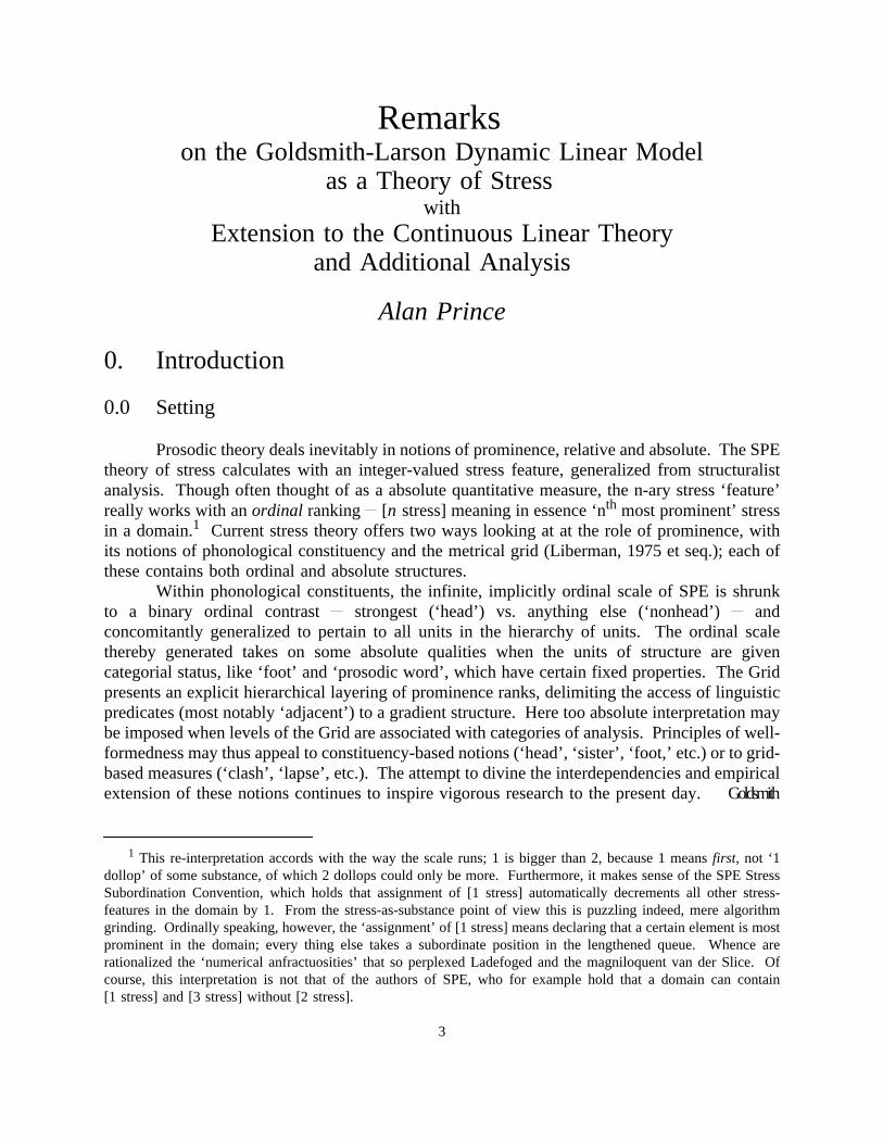
0. Introduction

0.0 Setting

Prosodic theory deals inevitably in notions of prominence, relative and absolute. The SPEtheory of stress calculates with an integer-valued stress feature, generalized from structuralistanalysis. Though often thought of as a absolute quantitative measure, the n-ary stress ‘feature’really works with anordinal ranking [n stress] meaning in essence ‘nth most prominent’ stressin a domain.1 Current stress theory offers two ways looking at at the role of prominence, withits notions of phonological constituency and the metrical grid (Liberman, 1975 et seq.); each ofthese contains both ordinal and absolute structures.

Within phonological constituents, the infinite, implicitly ordinal scale of SPE is shrunkto a binary ordinal contrast strongest (‘head’) vs. anything else (‘nonhead’) andconcomitantly generalized to pertain to all units in the hierarchy of units. The ordinal scalethereby generated takes on some absolute qualities when the units of structure are givencategorial status, like ‘foot’ and ‘prosodic word’, which have certain fixed properties. The Gridpresents an explicit hierarchical layering of prominence ranks, delimiting the access of linguisticpredicates (most notably ‘adjacent’) to a gradient structure. Here too absolute interpretation maybe imposed when levels of the Grid are associated with categories of analysis. Principles of well-formedness may thus appeal to constituency-based notions (‘head’, ‘sister’, ‘foot,’ etc.) or to grid-based measures (‘clash’, ‘lapse’, etc.). The attempt to divine the interdependencies and empiricalextension of these notions continues to inspire vigorous research to the present day.Goldsmith

1 This re-interpretation accords with the way the scale runs; 1 is bigger than 2, because 1 meansfirst, not ‘1dollop’ of some substance, of which 2 dollops could only be more. Furthermore, it makes sense of the SPE StressSubordination Convention, which holds that assignment of [1 stress] automatically decrements all other stress-features in the domain by 1. From the stress-as-substance point of view this is puzzling indeed, mere algorithmgrinding. Ordinally speaking, however, the ‘assignment’ of [1 stress] means declaring that a certain element is mostprominent in the domain; every thing else takes a subordinate position in the lengthened queue. Whence arerationalized the ‘numerical anfractuosities’ that so perplexed Ladefoged and the magniloquent van der Slice. Ofcourse, this interpretation is not that of the authors of SPE, who for example hold that a domain can contain[1 stress] and [3 stress] without [2 stress].

3

and Larson have recently put forth a model of prominence computation that differs considerablyfrom familiar prosodic theory (Goldsmith and Larson 1990; Goldsmith 1991, 1992, in press;Larson 1992). The model involves iterative computation of real-numbered prominence valuesin a spreading-activation network. Because the model is dynamic, and because the calculationprocedure involves linear equations, we will refer to it as the Dynamic Linear Model (DLM).In its current stage of development, the DLM does not aim to offer an account of the fullhierarchy of prosodic structure in a single network. It is used to locatepeaksof prominence ina sequence of units, making the contrast between nucleus and non-nucleus in the syllable whenits units are taken to be segments, between stress and non-stress when its units are taken to besyllables. (If the units were regarded as stresses, the model would distinguish primary fromsecondary.) The conceptual affinity is therefore with the metrical grid (as indeed Goldsmith hasfrequently observed), though without the extended hierarchy; one might say that the DLM offersa fresh perspective on matters handled by two adjacent rows of the grid, the most basic structureof relative prominence. In particular, the theory holds out the promise of obtaining a smooth andprincipled transition from intrinsic prominence at one level (e.g. syllabic) to derived prominenceat the next (e.g. stress) through its uniform, numerical treatment of prominence at all levels.

In Part I, we will explore the properties of the DLM as a theory of stress, drawing on andadding to the analytic results of Parts II and III. We will first present a qualitative assessmentof the model’s properties, avoiding formal details, so that readers can come to an understandingof the model’s linguistic import without having to master its algebra. We then turn to formalanalysis. We show that DLM is a discrete approximation to a critically or heavily dampedharmonic oscillator, exhibiting the relevant differential equations, which shed considerable lighton what the network actually accomplishes. We conclude with proof of the new claims madein the qualitative discussion.

First, some background.

0.1 How the DLM Computes

In the Goldsmith-Larson spreading-activation model of stress and syllable structure (DLM), thelinguistic string is represented as a network of nodes with mutual interconnection betweenneighbors. The network for a string of lengthn can be pictured like this, using arrows torepresent paths of influence:

(1) N1 N2 ... Nn 1 Nn

Each node is endowed with an unchangingbias, which represents sonority or weight, conceivedof as the intrinsic disposition of a segment or syllable to occupy a position of high prominence.Each node has anactivation level, which (because of the way it is derived) takes into accountnot only the node’s own bias but also theactivationof the node’s neighbors. The computationof activation is iterative: every node passes activation to adjacent nodes in each cycle ofcomputation, and the cycles repeat forever. The effects of node-activation are modulated byweightson the links between nodes. Goldsmith and Larson postulate that all leftward links havethe same weight (notatedα); similarly all rightward links have the same weight (notatedβ).Weights may be positive, negative, or even 0. The activation of a given node is updated by

4

weighting the activation on the adjacent nodes and summing the result with the node’s ownintrinsic bias. We can redraw the connection-diagram of the network to show the role of the linkweights and biases:

(2) Network Architecture

The updating procedure can be written out like this, using ak for the activation level ofnodek, bk for the intrinsic bias,α for the weight associated with leftward-moving activation,βfor the rightward weight:

(3) ak ← α ak+1 + β ak 1 + bk

This is a recipe for generating new activation levels for each node (left-hand-side), given thecurrent levels (right-hand-side). Notice that the activation of nodek itself (ak) does not enter atall into the calculation of the new level for nodek. One can think ofactivationas measure ofa node’s influence on its neighbors, and the fixed bias as a measure of a node’s influence onitself.2

The calculation starts with all activations ak set to 0. The update scheme (3) on the firstcycle of iteration gives each node an activation equal to its bias; serious computation then begins.(Usually serious, that is: if bothα andβ are zero, there is of course no neighborly interactionat all; and if all biases are zero, all activations remain perpetually zero.) All activations arerecalculated in each cycle of computation. But in favorable circumstances, it will happen thatthe set of activations will change less and less with each succeeding cycle, settling (in the limit,typically) on stable values that will repeat themselves without change. These stable activationvalues are theoutputof the network.

Since linguistic strings have various lengths and a network has but one, it is necessary todefine a notion ofmodelmore abstract than network. Let a model Mαβ = ⟨α,β, ⟩, where isthe set of string-networks of all finite lengths. We are interested in what the model makes ofevery possible sequence of node biases. Letb = (b1,...,bn), a vector (i.e. string) of biases,representing the assignment of some numerically-measured property to the syllables or segmentsin the string. Letb* be the string of activations ultimately attained by the computationalprocedure the result of setting the model to work onb. We can write

(4) b* = M αβ (b)

2 To emphasize the fact that a node’s current activation-level hasno influence on the immediate update of itsown activation, we might write: ak ← α ak+1 + 0 ak + β ak 1 + bk.

5

The function Mαβ produces its output by computing according the iterative scheme in eq. (3).For a model Mαβ to make anything at all of a string of biasesb, the iterative scheme must settleon a stable, finite value for the activation of each node. At this point of convergence orequilibrium, each new cycle of computation will produce an output exactly equal to its input. Theactivation of each node is stable and in a stable relation with the activations of its neighbors. Theera ofbecominghas come to an end; history is over; a node’s activationis a weighted sum ofadjacent activations and self-bias. For such a ‘fixed point’b* = (a1,...,an) we have

(5) ak = α ak+1 + β ak 1 + bk

At convergence, the ‘←’ is replaced by ‘=’. The stable activations of then nodes are describedin n equations like (5), one for each node. The equations portray the final activations, theak’s toward which a convergent networks tends, as a function of the network parametersα,β andthe values of the input bk’s, fleshing out the import of eq. (4). The function associated with amodel Mαβ is a set ofn linear equations inn unknowns, which can be solved explicitly, allowingus to use analytical methods to investigate the structure of the DLM (Parts II and III below).One useful basic result of such analysis is that we can determine exactly when parametersα andβ will produce convergent networks. Any Mαβ will converge for all inputs if, and only if,αβ≤ ¼ (Part II below). Outside this region, models fail to settle, exploding to infinity, or underspecial circumstances, entering oscillatory regimes.

0.2 Models and Theories

The output activation sequenceb* of a convergent model Mαβ counts as a linguistic descriptionwhen its numerical structures are interpreted with reference to linguistic constructs such as‘sonority’,‘syllable’, ‘stress’ and so on. For Goldsmith and Larson, it is the position of localmaximain the string, rather than absolute activation values, that determines the interpretation.3

When the nodes are taken to represent segment positions, with the biases representing sonorityvalues, then the local maxima in the output are interpreted as syllable peaks. If the networknodes are taken for syllables, with the biases representing weight or intrinsic (lexical) stressesor accents, then the local maxima in the output are stresses. A given model, plus a crucialinterpretive component that finds maxima, maps a string of segments to a string of syllables, ora string of syllables to a stress pattern or indeed any string of linguistic units with a numericalprominence structure defined on it — to a modified version of itself.

3 It is necessary to refine the notion ofmaximumat play here, since networks can easily produce equalitybetween adjacent nodes (v. Part III). While it might be sensible to regard a sequence like [1,2,1,1] as stressed onthe second node, it is not plausible that [1,2,2,1] should be viewed as completely unstressed, on a par with [1,1,1,1].We therefore introduce the notion ofquasi-maximum: a node is a quasi-maximum if it’s greater than at least one itsneighbors but neither neighbor is greater than it. Every maximum is a quasi-maximum, and in [1,2,2,1] both of the2’s are quasi-maxima.

6

Each Mαβ is a specific grammar of (an aspect of) prosody. The set of all such grammarsthen comprises a linguistic theory of that aspect of prosody. As with other such theories, thereare two general claims to explore about the success of the theory:

(A) Descriptive Inclusiveness. For any actual linguistic prosodic system (stress, syllablestructure), there is someα,β and some set of biases such that the patterns of the system aregenerated by Mαβ.

(B) Predictive Validity. Every parameter setting ofα,β, and biases describes an authenticlinguistic system.

Neither claim will hold up, of course, under scrutiny, but this is no reason to abandon theinvestigation. Exactly as with most other known theories, we work with relativized versions ofthe general claims.4 The theory may not be descriptively inclusive (A), but it does offer newdescriptions of complex phenomena (v. Goldsmith, Larson refs.). The theory may not bepredictively valid (B), but it does offer interesting, unexpected entailments (Part III below). Thiswill establish the significance of the approach in the minds of most serious researchers.5 TheDLM marks the first attempt to derive the characteristics of a rich, well-understood linguisticdomain from the behavior of a dynamical system, and deserves investigation not only becauseof such low-level empirical successes as can be obtained, but because understanding it will pointthe way toward deeper models as yet unimagined.

1. Qualitative Characterization of Stress in the DLM

1.0 How Patterns are Built Up

Despite the existence of descriptive overlap (an empirical necessity), which may stir direvisions of ‘notational variant’ or ‘mere implementation’ in the minds of some thinkers, theleading ideas of the DLM are quite distinct from those of symbolic theories. The constraints ofmetrical theory are imposed by what amounts to Boolean logic. ‘Do not place a new entry inthe grid if it would be level-adjacent to another entry.’ The DLM, by contrast, works throughaddition. A lone stress causes activation to spread throughout the string it sits in. If there areseveral stresses positive biases in the string, the global result is exactly thesumof the veryactivation-patterns caused by each independently, in the absence of the others. A stress does notsee other stresses, does not influence them in the way they send out their activation.6

4 According to reliable authorities, Quantum Electrodynamics does not require this dispensation. The downsideis that no one seems to know what the theory isabout a small price to pay in the circumstances.

5 This point of view, which emphasizes the value of ideas, is of course familiar from Chomsky’s remarks overthe years. Dissent from it is common in practice, under the constraints of advocacy and trepidation.

6 This is consequence of the linearity of the equations defining the computation performed in the DLM. Suchbehavior is of course characteristic of many familiar wave phenomena, which are controlled by linear equations; see§2 below for analysis of the DLM as a wave generator.

7

The metrical grid can be thought of as a Boolean network; a given node does not workfrom a weightedsumof the state of its neighbors and its own intrinsic bias, but evaluates thissort of information according to a scheme built up from Boolean connectives. This is notcommensurable with the additive method. To see this, consider the effect of a lexically-prespecified stress in a string. Assume that an iambic (minimum-first) pattern is to be developedfrom left to right (LR→); assume that the the fixed stress is in an odd position. Let us writeχfor the lexical stress and its consequences. The following grid fragment would result

The LR→ unfolding of the pattern results from a local interaction between adjacent gridpositions. What’s important is that the fixed lexical stress puts an absolute end to the influenceof the stress that precedes it; a new calculation begins.

In the DLM, there is no such curtailing of influence. Each stress sends its activation outinto the unlimited distance, bouncing and echoing off the ends of the string forever, and thatwave of activation rolls through anything in its way. A lexical stress will make itself felt becauseits own waveaddsto the others, not because it inhibits their propagation.

The DLM is thus capable of very significant long-distance effects. If for example, theleftward weightα is 1 while the rightward weightβ is 0, the bias of any node is simply copiedonto every node to its left. If the leftward weightα is 1, then positive and negative copies ofa node’s bias spread leftward in an alternating pattern, the immediate neighbor receiving anegative copy, the next one over receiving a positive copy (since 1× 1 = +1), and so on. Ahigh-activation node will strongly suppress the ultimate activation achieved by alternate nodesto its left.7 To see this at work, consider the following example, in whichβ = 0 (no rightwardtransmission at all) andα = 1 (giving alternating waves going leftward).

(6) Wave Cancellation

α = 1, β = 0 N1 N2 N3 N4 N5 N6

Biases 0 0 1 0 0 1

Wave from N3 1 1 1 0 0 0

Wave from N6 1 1 1 1 1 1

SUM of Waves 0 0 0 1 1 1

The alternating wave pumped by the bias on Node 6 cancels the wave associated with Node 3.

7 This raises an interesting question: is there a setting of parameters such that a node can annihilate itself? Theanswer is no. We need only consider the case where the network has just one non-zero bias. Recall that the initialcondition of the net is all activations 0. If in the process of iteration we arrive at a state where all activations are0, we are back at the beginning and are doomed to repeat the cycle endlessly. But forαβ ≤ ¼, the networkconverges on a fixed output and has no oscillatory regimes.

8

Phenomena of this character have not been noted in the linguistic domain, of course. The DLM(and numerical approaches generally) offer exponential decay of amplitude with distance as away of controlling such influences. As just seen, and as will be seen in more detail in §2 below,the rate of decay that can be managed by the DLM is not always dazzlingly fast (indeed it is notsimply exponential, but somewhat faster or slower that an exponential with the same decay factorwould be). Further, the DLM is equally capable of expressing exponentialexplosionof influencewith distance. This fact merely highlights the generality of the explanatory problem that isevident in table (6): not every region of the parameter space is one that stress patterns live in.

The fundamental conceptual issue is whether stress patterns ever add not only in thedramatic sense of total cancellation, but in any sense at all. This marks an important dividingline between the symbolic paradigm and the particular quantitative approach embodied in theDLM. We will argue that the evidence, from relatively subtle details of the DLM, indicates thatthey do not. However, in pursuit of this question we will uncover a variety of unexpectedproperties, some of which offer new perspectives on classical descriptive problems.

1.1 Culmination and the Barrier Models8

Since complicated input is processed by summing its simple components, it is instructiveto examine the very simplest building blocks out of which complex structures can be constructed.These are the bias-strings that are zero everywhere except for a single 1. Let us use the notation

nek to represent a string of lengthn, with 1 as bias on the kth node, zero bias elsewhere.9 Itshould be clear that from the full set of such basic strings, any bias sequence whatever can bebuilt up by addition and by multiplication by a numerical scaling factor.10 For example, theactivation string (2, -3) is just 2×(1,0) -3×(0,1). Once we understand how the DLM treats theek’s, we are well-positioned to understand its general behavior.

These basic constructional units can be thought of as syllable strings with a single lexicalaccent. An input string with two accents such asσ́σσσσ́σ is just the sumσ́σσσσσ + σσσσσ́σ.

Numerically, this is (1,0,0,0,0,0,0) (0,0,0,0,1,0). The result of applying any model toσ́σσσσ́σis exactly the same as applying the model toσ́σσσσσ and to σσσσσ́σ separately and thensumming the individual results. Furthermore, the influence of an accent can be magnified ordiminished or inverted by multiplying the basic string by some constant factor, say 1.2×(σ́σσσσ)or 3×(σ́σσσσ). We can mix multiplication and addition to get objects likeσ́σσσσ + 1.2×(σσσσ́σ). In this way a string of syllables with any conceivable numerically-representable structure can be analyzed as the weighted sum of the basic one-accent strings, theek’s, and the processing in the models respects this analyis completely.

8 The formal analysis supporting the assertions made here is found in Part III below.9 We will be able suppress the pre-subscript, fortunately.10 To add strings, add the elements in corresponding ordinal positions, first with first, second with second, and

so on, just as in table (6). To multiply a constant times a string, multiply each position in the string by the constant.

9

Let’s use the notationek* to represent the result of processingek in a some model Mαβ.The model Mαβ itself can be thought of as a kind of stress rule; the stringek* is the output ofthe rule, given an underlying formek. (One caveat: the absolute activation values have nomeaning, only the location of quasi-maxima among them; the actual output of the DLM shouldbe a string of, say, 0’s and 1’s, demarcating the quasi-maxima.) Output based on complex inputis analyzable as the weighted sum of output based on simple inputs: if (b1, b2,...) is a string ofbiases, then we can write this basic observation down as follows:

(7) Analysis of Complex Input

(b1, b2, ...) = b1×(1, 0, ...) + b2×(0, 1, ...) + ... = b1e1 + b2e2 + ...

Mαβ(b1, b2, ...) = b1×Mαβ(e1) + b2×Mαβ(e2) + ... = b1e1* + b2e2* +...

Knowledge of the characteristics of theek* will therefore open the doors to understanding thenature of the DLM.

The fundamental properties of theek*, established in Part III, are these:

1. Alternation of Sign. The nodek has positive activation. Ifα is negative, thenalternate nodes precedingk have negative activation. Ifβ is negative, then alternate nodesfollowing k have negative activation. In this way, binary alternation of stress emerges.

2. Culmination. If α andβ are both positive, then all activation is positive, and there isone and only one maximum value (which may indeed be shared between two adjacent nodes).Such models assign one stress to a string (or at most two on adjacent syllables, if each quasi-maximum counts as a stress).

3. The Barrier Property. Exactly where the culminative maximum falls whenα andβare positive is matter of some interest. With simple input like theek, the result is particularlystriking: For a given positiveα andβ, the maximum onek* falls no further than a certain fixeddistance from one edge.

We can think of the nodep beyond which there is no surface accent as a kind of barrierto the transmission of influence. If the lexical accent lies at orinside the barrier that is, onnodep or between nodep and the relevant edge then the lexical accent itself is realized. (Theunit bias on nodek of ek causes a a maximum to surface on nodek of ek*.) If, however, thelexical accent lies beyond the barrier, the output maximum ends up on the barrier node itself andnot on nodek. Here, the bias on nodek of ek leads to a maximum on nodep of ek*. As anexample, consider the input-output map of a model with a barrier on node 3:

(8) Barrier on Node 3Input Outputσ́σσσσ → σ́σσσσσσ́σσσ → σσ́σσσσσσ́σσ → σσσ́σσσσσσ́σ → σσσ́σσσσσσσ́ → σσσ́σσ

10

The Barrier Property is remarkable in a couple of respects. First of all, the location ofthe barrier depends only onα andβ the basic parameters of the model and not at all on thelength of the input string.11 The barrier’s position is measured in absolute terms from an edge,not by some function relativized to length. This is of course highly desirable, since dependenceon the absolute length of a string is not observed in language. Second, the Barrier Propertyreflects a kind of subtle behavior that is common among stress and accent systems: accentrecedes as far back as it can from an edge (typically the end) within some window (oftensomething like 3 syllables), but within that window a lexical marking or special rule supersedesthe recessionary trend. Stress or accent will never be foundoutsidethe window, beyond thebarrier. Examples of this general type blurring details would include Greek, Latin, Pirahã,English, and Spanish (for recent discussion, see Kager 1992).

The Barrier Property emerges unexpected and uncoaxed from the basic design of theDLM, providing a kind of explanation-from-first-principles for a much-discussed phenomenon.Results of this character, without real parallel in competing systems, intensify the interest of thewhole project.12

Further investigation of the Barrier Property indicates that the result is incomplete invarious ways, however. First of all, a barrier can be placed onany node (measured from anedge), not just on the 2nd or 3rd unit from the edge, the commonly-encountered positions. Toencourage a feel for this, let’s look at some actual parameter settings and their effects. Theimportant factor in barrier-placement turns out to be the (positive) square root of theratio of αandβ, (α/β)½, which we will call r. If we setαβ = ¼, we get very simple solutions to the DLM,which allow for explicit statement of the conditions on barriers. Let’s call all Mαβ for whichαβ = ¼ the ‘Canonical Models’. (Note that fixing the product of the two parameters leaves theirratio completely free to vary, so the full range of behavior is still exemplified; no generality islost in focussing attention on the Canonical Models.) The model with a barrier atp we will calla ‘p-Model’. The following table shows how things come out:

11 Whence the celebratory titleTheorema Egregiumapplied to Thm. 13 of Part III below.12 The Barrier Property entails that the input-output function is not invertible: given the output array marking

the location of extrema, one cannot in general point to a single input that would underly it, even when one knowsα and β. For example, surface accent on the 3rd syllable in a 3-Model could come from anyek with k ≥ 3. Innatural language systems of this sort, the position of underlying accents in morphemes and strings of morphemesis arrived at by paradigmatic (not syntagmatic) arguments, often complex.

11

(9) Barrier Location in the Canonical Models, measured from the beginning

Model # Range ofr Range Length

1-Model ∞ to 2 ∞

2-Model 2 to 1.5 1/2

3-Model 1.5 to 1.33+ 1/6

4-Model 1.33+ to 1.25 1/12

j-Model j/(j 1) to (j+1)/j 1/ j(j 1)

∞-Model 1 0

A entirely parallel situation obtains for cases where the barriers are reckoned from the end ratherthan the beginning of the string. Let’s call these the (p)-Models.

(10) Barrier Location in the Canonical Models, measured from the end

Model # Range ofr Range Length

1-Model 0 to .5 1/2

2-Model .5 to .66+ 1/6

3-Model .66+ to .75 1/12

4-Model .75 to .8 1/20

j-Model (j 1)/j to j/(j+1) 1/ j(j+1)

∞-Model 1 0

The endpoints of the ranges for the finite barriers are not to be included in the range ofr. (Atthe endpoint between the k-Model and the (k+1)-Model, nodesk and k+1 share the maximalvalue.) In the∞-Model, everyek* has its maximum atk, since everyk is less than∞, so thatthe surface form exactly reflects the lexical specification. The∞-Model behaves identically.

The range ofr runs from 0 to∞ (excluding the endpoints). But all the action in theCanonical Models takes places in the range ½ 2. Forr < ½, everyek* has final stress; forevery r > 2, stress is initial on everyek*.

Notice that the length of the rangedecreasesas the barrier recedes from the edge (here,from the beginning of the string). It might therefore be possible to address the problem ofunlimited barrier-distances to establish the primacy of the 1-,2-, and 3-Models by coarseningthe DLM’s ability to set parameter values, introducing some quantization into the model, as it

12

were. Also worth exploring would be the possibility of arranging things so that the primacy ofthe lower distances was a mere statistical artifact.

A second, deeper problem is that the Barrier Property holds only of the processing of theek and not generally over all input. With prosody in mind, one would hope that in the case ofmultiple accents, the effect would be to maximize the leftmost or rightmost inside the barrier. Butnothing of the sort emerges. Instead, the presence of even one other stress can introducesignificant effects of string-length into the calculation. Consider the set of input stringsbeginning σ́σσ́.... Setting αβ = ¼, and (α/β)½ = 1.4, to produce a 3-Model, we find thefollowing input-output map:

σ́σσ́ → σ́σσσ́σσ́σ → σ́σσσσ́σσ́σσ → σσ́σσσσ́σσ́σσσ → σσ́σσσσ

Surface accent hits the leftmost underlying accent for 3- and 4- syllable strings, but settles on anunfortunate compromise between the underlying accents in longer strings: syllable 2,underlyingly unaccented but sitting right between the two basic accents.

A sense of how this happens can be garnered from a direct comparison of the innerworkings of the 4- and 5-syllable cases, presented in the following two tables (all valuesrounded).

(11) Four Syllables: αβ = ¼, r = 1.4. Input: /σ́σσ́σ/

Biases: 1 0 1 0

Wave from N3 1.57 2.24 2.40 .86

Wave from N1 1.60 .86 .41 .15

SUM of Waves 3.17 3.10 2.81 1.00

(12) Five Syllables: αβ = ¼, r = 1.4. Input: /σ́σσ́σσ/

Biases: 1 0 1 0 0

Wave from N3 1.96 2.80 3.00 1.43 .51

Wave from N1 1.67 .95 .51 .24 .09

SUM of Waves 3.63 3.75 3.51 1.67 .60

13

This length-dependent contrast is a direct consequence of the additive mechanism thatpowers the DLM. Its failure to match reality provides us with compelling evidence that stresspatterns do not add together (as indeed Boolean symbolic models predict). We are left with theconclusion that the Barrier Property is a remarkable result which points in the direction of newmodes of explanation, although richer dynamical assumptions are evidently required to actuallyarrive at a sound alternative to current theory.

1.2 Quantity-Insensitivity

Analyzing the behavior of the mono-accentualek’s lays the foundation for understandingcomplex patterns. Among these, one is of obvious interest: the string in which all biases areequal. This provides the natural representation for quantity-insensitive prosody, in which the inputstring is analyzed as a sequence of undifferentiated syllables. Since there is no reason toconsider any other activation level besides 1, let us focus on a string we will call∑, in whichevery unit has 1 as bias. The string∑ is the sum of allek’s of a given length. We will base ourassertions on formal analysis of the Canonical Models, whereαβ = ¼. (Details are found in §3below.) Recall that it is theratio not theproductof α andβ that is crucial to determining theeffect of the model on its input. Imposing other conditions on the productαβ adds nothing tothe range of patterning of maxima, so long as 0 <αβ < ¼.) Here again will writer = (α/β)½.

We will examine the two fundamental patterns that can be imposed on∑* culminationin a single maximum value (positiveα and β); and alternation of maxima (α and β negative).We will find a number of effects that are quite interesting in themselves, but which indicate thatthe extremal patterns of the DLM are rather different from those of linguistic prosody.

1.2.1 Culmination in∑*

For theek* the surface forms of theek the location of the maximum is determinedby r alone; hence the desirable independence from the string lengthn. In ∑*, however, theculminative position isalwaysa function of bothr and n. As length increases, the effects ofstring lengthn diminish and indeed disappear in the limit: there the culmination principlebecomes strictly a function ofr and is identical to that relevant to theek*. But for short strings(like those witnessed in languages), strong length effects are unavoidable.

The overall pattern works like this. Forr less than ½, the maximum falls on the last unitof the string, just as13 for the ek*. For r = 1, the theoretical maximum falls exactly at themidpointof the string: (n+1)/2. This is, of course, an extreme case of length-dependence. If thestring is of odd length, then there is a node sitting at this point which receives the maximum.If the string is of even length, then the abstract midpoint is flanked by two actual nodes, whichshare equally in the highest activation in the string. This behavior is highly nonlinguistic. Nolanguage has a stress rule putting stress right in the middle of the string; the notion ‘exact

13 Since withr < ½, we have end-stress on everyek*, with a steady rise to that maximum over the entire string,it is clear that adding up all theek*’s of a given length will put a maximum on the last node of the sum.

14

middle’ is surely not available to grammar. And no language has a rule puttingtwo adjacentstresses across the midpoint of even-length strings.

If we fix r somewhere between ½ and 1, the maximum will lie between the end of thestring and the midpoint. As string-lengthn increases, the maximum drifts toward itsr-dependentlimit position. Let us look at some examples to clarify how this works.

Supposer = .6. The maximum is final for strings of length 2 and 3, and penultimate forlonger strings.

Supposer =.7. The maximum is final for length 2, penultimate for length 3-8, andantepenultimate for longer strings.

Supposer = .8. The maximum is final for strings of length 2, penultimate for length 3-5,antepenultimate for length 6-10, pre-antepenultimate for length 11-82, and finally fifth-from-the-end for length 83 and above.

As r runs between 1 and∞, the same pattern repeats in mirror image, reckoning maximalposition from thebeginningof the string to the midpoint.14

These findings show that∑ is essentially unmanageable as a model of a syllable-stringthat is to receive one accent by phonological rule encoded inα, β values. The accent cannot bemade to sit still as length varies, except at the very edges.

1.2.2 Alternating Patterns in∑*

Whenα andβ are both negative, eachek* shows a binary alternating pattern of positiveand negative activations, anchored at nodek, which is positive. Adding up all theek* to get ∑*gives rise to alternating patterns of maxima and minima (with exceptions to be discussed below),providing a natural model of familiar patterns of alternating stress. Here considerable regionsof length-independence are to be found.

As in standard prosody, there are crucial differences in behavior that depend on the parity(oddness/evenness) of the string, rather than on its absolute length. These will allow us toconstruct an account of the four basic alternating types: iambic and trochaic, right-to-left andleft-to-right.

The basic facts are these:(i) Odd-length∑* are stable throughout the entire range ofr: they have maxima on

all odd-numbered nodes.(ii) Even-length∑* show three classes of behavior:

(a) Forr greater than approximately 1.211, maxima fall on even-numbered nodes.(b) For r less than approximately .826, maxima fall on odd-numbered nodes.(c) There is a transitional region between .826 and 1.211 (roughly) in which there

are length-dependent failures of strict alternation.

14 Here again, most of the road to∞ is barren. The maximum falls on the first node forr > 2, regardless ofstring length. As with theek*’s, all the crucial action in the Canonical Models is compressed into the range ½ 2.

15

Let’s put aside the transitional region for the moment. In the secure arear < .826, allmaxima in all strings fall on odd-numbered nodes. This is the correlate of trochaic, LR→, withmono-syllabic feet stressed. A more exact parallel is available in the pure grid theory of Prince1983, which like the DLM does not recognize constituents: build the gridPeak-First, LR→.

In the secure arear > 1.211, maxima fall on even nodes in even-length strings, odd nodesin odd-length strings. Greater perspicuity is attained when we count node-numbers from the endrather than the beginning: then maxima fall always on odd-numbered nodes. (This is exactlythe mirror image of the pattern forr < .826.) The approximate correlate in foot theory is:iambic, ←RL. Again the more exact parallel is the grid-theoretic rubricPeak-First,←RL.

The processing of∑ yields two alternating patterns, both peak-first, which would beassigned in opposite directions in a directional theory. Two other possible patterns remain:trough-first in either direction, in grid terminology; or iambic, LR→ and trochaic,←RL (thenearest correlates in foot theory). These must be attained by applying the models to∑, i.e. bymultiplying the just-described patterns by 1, which will exchange maxima and minima, asGoldsmith has suggested (Goldsmith in press).

The results of this survey can be tabulated as follows:

(13) Classification of Binary-Alternating Systems

∑* ∑*

r < .826 Peak-First≈ trochaic

LR→ Trough-First≈ iambic

LR→

r > 1.211 Peak-First≈ iambic

←RL Trough-First≈ trochaic

←RL

This system is of course heir to the complaints registered against the original grid-theory,which induced the same classification. At issue is whether the rows and the columns of the tabledefine natural groupings (Hayes 1985). The vertical categoryPeak-First(or, equivalently,∑*-based) mixes iambic and trochaic, as does the categoryTrough-First(or ∑*-based). Similarly,the horizontal category LR→ (small r) mixes the two rhythmic types, as does the category←RL(big r). Modern theory has insisted on the primacy of the iambic/trochaic distinction, which islost in grid-type classifications that recognize only the whole string and not the foot as theessential prosodic domain. Regardless of such deeper empirical problems, it is notable that theDLM is able to generate a fair facsimile of the range of alternating systems, and in a stable,length-independent way.15

More interesting, perhaps, and more disconcerting is the existence of the transitionalregion between the two stable zones. The greater interest springs from the fact that the

15 Multiplying bias by 1 cannot be recommended as a generally allowable procedure, however, inasmuch asit would turn high-bias items like heavy syllables into rejectors rather than attractors of stress.

16

transitional region is a distinctive property of the DLM not shared by known symbolic theories,and furthermore the kind of property that is intrinsic to the mechanics of the DLM. Because theDLM is linear, small changes in parameters will result in small changes in behavior; there canbe no catastrophes, singularities, or sudden reversals. Consequently, two opposite forms ofbehavior for example, what is describable as LR→ vs.←RL stressing of string must alwaysbe linked by a gradual transition, as one set of additive wave components grows in strengthrelative to its competitors.

In the transitional region, there is a one-by-one flipping of maxima and minima asrincreases, going through a stage of complete equality between each adjacent pair of nodes.(Recall that odd-length strings are stable, so only even length strings are affected.) This processis portrayed iconically in the following display, which follows the transition of∑* from LR→Peak-First to←RL Peak-First.

Transition in 6-unit∑* LR→

←RL

r

X x X x X x 6 0 Small r

X x X x X X 5 1

X x X x x X 4 2

X x X X x X 3 3 r = 1

X x x X x X 2 4

X X x X x X 1 5

x X x X x X 0 6 Big r

The string passes through every mixture of left-to-rightness and right-to-leftness. In the process,various patterns with adjacent quasi-extrema are generated. A particular interesting case occurswhen r = 1; the equal quasi-extrema straddle the exact midpoint of the string.

A further important characteristic of the transitional region islength-dependence: a givensetting ofr can produce rather different patterns in strings of different length. For example, taker = 1.2. The general pattern is Peak First,←RL (≈iambic). But in strings of length 6 and 8 thefirst ‘foot’ is inverted that is, these lengths show a mixture of (what are usually thought of as)directionalities: the first two units are LR→, the remaining units←RL. The set of patterns lookslike this:

(14) Length Dependence in the Transitional Region of the Parameter Space

Length Stress Pattern2 σσ́4 σσ́σσ́6 σ́σσσ́σσ́8 σ́σσσ́σσ́σσ

17

10 σσ́σσ́σσ́σσ́σσ́

Empirically, of course, the kind of behavior seen in the transitional region is unattested,both in the patterns themselves, with their adjacent quasi-extrema (particularly quasi-maxima),and in the dependence on absolute segmental length. Indeed, it is even-length strings that arestable in the natural world, with odd-lengths falling under special constraints that deal withunpaired syllables. The existence of the transitional region is a direct consequence of the model’sdesign: its linearity. We are led to the conclusion that stress patterns do not, in fact, combineadditively; and that the descriptive success of the basically Boolean-based symbolic theoriesentails that dynamical models require more complex design if they are to achieve a better matchwith reality.

1.3 Summary of Discussion

The DLM achieves significant success in modeling basic features of stress patterns innatural language. The models in whichα andβ are both positive give an account of culminativepatterns, those with just one local maximum. For mono-accentual input, such models show theBarrier Property, which limits the location of surface accent to an edge-most window.Underlying accents at or beyond the barrier give rise to surface accent at the barrier, while anaccent inside the barrier gets realized in its underlying position. Location of the barrier iscounted from an edge, and is independent of string length. Unfortunately, the Barrier Propertyholds only of mono-accentual input; the presence of even one more underlying accent can leadto length-dependent pathologies.

The quirks of multi-accented input in the culminative regime are clearly visible in stringswith uniform activation throughout. Examining∑, the sum of all mono-accentual input strings,with activation 1 everywhere, we found that placement of the culminative maximum in the output∑* was thoroughly length-dependent. Memorably, forr = 1, the culminative accent falls rightin the middle of the string and is not measured from an edge at all. For even-length strings thisentails a shared quasi-extremum over the middle two nodes. The location of the maximum in∑* only becomes stable for long string-lengths; the exact length at which stability is achieveddepends onr. With increase of length in shorter strings, there is a drift of the maximum towardits asymptotic position, the location of which is a function ofr. Because of the phenomenon oflength-dependent stress-placement, the input string∑ turns out to provide a poor model ofquantity-insensitive culmination.

When α and β are both negative, the entire Prince 1983 classification of alternatingpatterns is generable in a length-independent fashion, if uniform negative activation is admitted.Between two regions of parametric stability, there is a transitional zone in which unattesteddouble-extrema patterns adjacent quasi-maxima (stresses) and and adjacent quasi-minima(unstresses) are produced, in a length-dependent fashion.

The treatment of alternation raises a fundamental question. Since there are only 4 usefulcells in the table indeed, only 2 cells are differentiated byr-values, the other 2 being generatedby the device of multiplying the input by 1 do we really want or need continuously manyparametric values to describe them? One clear justification for scalar parameters is the modeling

18

of scalar reality: but the basic interpretive assumption that only extrema are significantquantizes the output of the model, binarily. There is, nevertheless, a more subtle justification,of a type that has been argued by Paul Smolensky in a broader context (Smolensky 1988, forexample). Some types of behavior emerge from the very way that the model computes; theirexistence is diagnostic of a certain computational modes. Such behaviors can often be forcedfrom competing models, but if they are inevitable, we praise the models that have them forachieving explanation-from-principle. We praise them, that is, when the behaviors mirror reality;in the contrary situation, we are likely to be more circumspect. The computational assumptionsof the DLM lead to desirable results, like the Barrier Property and the ability to modelalternation, but they leave undescribed many basic patterns (e.g. edgemost accent wins) and leadjust as directly to length-dependence, to unattested gradual transitions between sharply definedcategories, and to additive compromises that are not characteristic of real systems. Although weare forced to the conclusion that stress patterns donot add (as current theory predicts), we mustrecognize that the DLM marks a real advance in the direction of finding new principles oflinguistic form, and therefore deserves careful analysis and vigorous extension.

19

2. The Continuous Linear Theory of Stress.

2.0 Background16

The DLM computes according to the following iterative scheme, repeated from (3):

(15) ak ← α ak+1 + β ak 1 + bk

This can be more concisely formulated in vector notation:

(16) a ← Wn a + b

Herea is the vector of node activations (initially0), b is the vector of fixed biases (the input tothe scheme), andWn is an n×n tridiagonal matrix with 0 on the main diagonal,α on thesupradiagonal andβ on the subdiagonal. Suppose thatαβ ≤ ¼, so that the iteration convergesfor any b. Let b* represent the ultimate activation vector (the fixed point) that the iterationsettles on, given a particularb. In the limit, we have:

(17) b* = Wnb* + b

This can be re-written like this:

(18) (I W n)b* = b

Or, more usefully,

(19) b* = ( I W n)1 b

Inverting the matrix (I W n) will immediately give the modeling function Mαβ that associatesinputsb with outputsb*.

Since Mαβ is linear it is sensible to inquire about its effects on the canonical basis vectorsek, which have 1 in the kth coordinate and 0 elsewhere. It turns out that two formulas arerequired forejk*, the jth coordinate of Mαβ(ek): one for those coordinatesprecedingthe kth, andanother for thosefollowing the kth. (The formulas agree onekk.)

Let us call the formula for the coordinates precedingk, the ‘Initial Wave’, since it can bethought of as presenting samples from a wave standing over the initial segment of the string,from node 1 to nodek. Similarly, let us call the formula for the coordinates followingk, the‘Final Wave’.

The general solution involves a certain amount of complication, which we will sweepaside forthwith, but it is worthwhile to exhibit the formulas.

16 Proofs of assertions made here about the DLM and further details are found in Part III below.

20

We introduce a parameteru, sensitive to the productαβ, defined as follows:

(20) 4αβ cosh2 u = 1, u ∈

Recall that we have a parameterr, sensitive to the ratioα/β.

The parameterr is either positive real ori times a positive real. To state the solutions concisely,let us define the following functions:17

(21) Uk(u) = sinh (ku) / sinh (u)

We have then forejk*,

(22) Initial Wave.

(23) Final Wave

Our interest will center on the conditions that prevail whenα andβ agreein sign; indeed,we will focus on the models obtained when the weight parameters are subject to the constraintαβ = ¼, which putsu at 0. These we refer to as the ‘Canonical Models’. The relevant formulasfor ejk* simplify greatly: observe that asu → 0, Uk → k, eliminating all reference to sinh.Since the extremal behavior of the Canonical Models is identical in the relevant respects to thatof the related models for whichα andβ are either both positive or both negative, and since onlythe extremal behavior has empirical interpretation, we lose nothing.

17 These are just the (k-1)st Chebyshev polynomials of the second kind applied to the argument cosiu. Thestructure of the DLM is tied up in various ways with that of the Chebyshev polynomials for example, theChebyshev polynomial of the first kind Tn+2 has its extrema atλk/(4αβ)½, where theλk are the eigenvalues ofWn.The figuren+2 shows up because the networks of DLM implicitly run between node 0 and node n+1, which alwayshave 0 activation. Thanks to András Kornai for directing me to the Chebyshev polynomials.

21

In the Canonical Models,α andβ are interdefinable, so there is really only one weightparameter,r.

(24) The Weight Parameter in the Canonical Models

The leftward weight is ±r, the rightward weight is ±1/r, wherer > 0, and the symbols ± areinterpreted uniformly so as to ensureαβ = +¼. (We do not admitr = 0, i.e.α = 0.) The basiciterative scheme for the Canonical Models comes out like this:

(25) ak ← ½ (±r ) ak+1 + ½(±r ) 1 ak 1 + bk

The solutions for the models take these forms:

(26) Initial Wave in the Canonical Models

(27) Final Wave in the Canonical Models

2.1 The Continous Linear TheoryIf all time is eternally presentAll time is unredeemable.

Burnt Norton

To move to the continous theory, we need to replacej ∈ Z+ with x ∈ . We will alsowant to deal withρ =def log (±r) rather ±r itself. For conciseness, we writeN for n+1.Separating out the bits that depend onx from those that do not, we have

(28) Initial Wave

(29) Final Wave

Notice that these both take the form of the product of a linear term with an exponential term.

22

It is worthwhile to examine the weight parameters. The network parameter ±r may bepositive or negative. As is clear from equations (26) and (27), withr there is alternation in signin ek* spreading out in both directions from nodek (which is positive). Theamplitudeof theactivation is the same, of course, as for +r. The +/ split onr divides the world into single-maximum, culminative patterns (+r) and alternating patterns (r).When the weight parameter isr, ρ is complex:

since log ( 1) =iπ (picking a handy branch of the logarithm function). The effect on thefunctions I and F comes from the exponential term, which expands as follows:

For integer x, this boils down to cos nπ = ( 1)n, creating alternation of sign, as desired.The parameterr also induces an important further split in behavior. Forr > 1, the

amplitude of the Final Wave falls steeply fromk to n. This is in part becauser k j decreases asj grows. (Equivalently, the exponential eρx in I and F decreases as x increases. Note that logr = Re(ρ) > 0.) Supporting the decrease in the exponential term is the fact that the linear term(N x) in the Final Wave is both positive and decreasing betweenk and n; hence the fall.

The Initial Wave, on the other hand, will show more interesting behavior: the exponentialterm still decreases, but the linear term merelyx increases. The Initial Wave may thereforeinclude amaximumin amplitude somewhere inside the span running from 1 tok.

If r < 1, this pattern of effects occurs in mirror image. This is evident from the fact therightward weight factor 1/r is the reciprocal of the leftward weight factorr. As the leftwardfactor ranges from 1 to∞, the rightward factor ranges from 1 to 0, and vice versa. In the logdomain, the contrast is between positive Re(ρ), with r > 1, and negative Re(ρ), with r < 1. Thisperfect symmetry means that we only need to focus on one interval or the other. Resultsobtained in one interval transfer immediately to other, reversing the sense of the string (i.e.treating the end as the beginning and counting node-numbers from right to left.)

For simplicity of discussion, but without loss of generality, we impose the restrictionr ≥ 1. In the log domain, this means Re(ρ) ≥ 0. In short, we will be looking at the followingtwo cases:18 ρ = log r and ρ = log r + iπ, with log r ≥ 0.

18 Recall from §1 that all the maximum-shifting asr varies is confined to the interval [½,2]. Outside thatinterval the maximum falls on the edge-most node. Taking a generous view of things, we need allow no greaterrange forρ than [-1,1] to get all significant behavior. Eliminating mirror-image redundancy, we have 0≤ ρ ≤ 1.

23

2.2 Towards The Continuous Theory

The functions I(x, k) and F(x, k) are immediately recognizable as solutions to thefollowing differential equation:

(30) (D + ρ)2 ψ = 0

The general solution is as follows:

Arriving at I(x, k) and F(x, k) requires setting appropriate boundary conditions that determine thefree constantsc1 andc2. There are two important conditions. First, the Initial and Final Wavesvanish at their outside boundaries, pointsx = 0 andx = N respectively. Second, the two wavesmust agree at pointk in the string.

(31) Essential Boundary conditions.a. I(0,k) = F(N,k) = 0b. I(k,k) = F(k,k) > 0

These conditions determine I and F up to a multiplicative constant; to get an exact result, weneed to pick a value for I(k,k) = F(k,k). The choice here is of no great significance, since theextremalbehavior of I and F is unaffected by multiplying them by a positive constant. If wewant the solutions to be identical to the values computed by the discrete network, we must pick

a choice that might not otherwise recommend itself.Equation (30) describes thecritically-damped harmonic oscillator. The prototypical

physical model of a harmonic oscillator goes likes this: imagine a mass attached to an anchoredspring; pull the mass some distance in the direction away from the rest point; at t = 0 release themass. There is a function f(t) that describes the displacement of the mass after its release, asolution to a 2nd order differential equation derived from Newtonian considerations. Withdamping, the mass does oscillate freely, but is itself in contact with some damping mechanismthat applies a resistanceρ to the motion. In the case ofcritical damping, the differential equationthat governs the oscillation simplifies to (30). The mass does not oscillate at all; displacementdecreases steadily with increasing time and asymptotes out at the 0 or equilibrium position(e ρt → 0 as t→ ∞ for positiveρ). See fig. (1) at the end of Part I for a graph of this courseof events.

The stress-theoretic application is quite different in character and requires a rather broaderperspective on the critical damping function. The physical application assumes an initial stateof affairs the mass displaced and unmoving before release, i.e. f(0) = A, f′(0) = 0, and theequation describes what happens as time moves forward. By contrast, the stress application

24

assumes that conditions are known at both edges of the domain under scrutiny (these beingpositions 0 andk for the Initial Wave, positionsk and N for the Final Wave), and uses theequationto calculate the location and amplitude of a displacement that would lead to these edgeconditions, given the value ofρ.

The effects of this ‘displacement’ must be conceived of as running both forwards andbackwards in time. Suppose, for example, that we are looking ate5*. The parameterρ can bechosen so as to put a maximum on the third node;ρ = will do the job exactly. This maximumis the analog of the initial displacement that sets off the spring apparatus. But we track itseffects not only forward in time to nodek, but also backward in time through nodes 2 and 1, andindeed to node 0, where displacement vanishes.

Fig. (2) at the end of Part I shows the generic shape of an Initial Wave under theconditionρ real (and positive, as agreed on). It has three notable characteristics.

(a) I(x, k) has its maximum atx = 1/ρ.(b) I(x, k) → ∞ asx → ∞.(c) I(x, k) is strictly positive for allx > 0, approaching 0 as an asymptote asx → ∞.

Property (b) is interesting: it shows that the ‘damped’ linear oscillator is damped in only onetemporal direction. Running time backwards past the maximal displacement, the wave’samplitude decreases without bound asx (‘time’) heads toward ∞. Observe that for complexρ,with an alternating pattern, Fig. (2) traces the envelope of the relative maxima of the real partof the function.

Fig. (3) shows the generic shape of theFinal Waveunder the same conditions onρ. Thenotable characteristics are these:

(a) F(x, k) has itsminimumat x = N + 1/ρ.(b) F(x, k) → ∞ asx → ∞.(c) F(x, k) is positive for allx < N. At x = N it goes negative, and heads back

toward 0 after its minimum, so that F(x, k) → 0 asx → ∞.

Note that the Final Wave has the same basicshapeas the Initial Wave. To get the FinalWave’s shape, turn the Initial Wave upside down (reflect throughx-axis) and shift it rightwardso that the 0-crossing is atN. (It is also multiplicatively scaled.)

We are now in a position to characterize the behavior of the DLM in terms of the thecritical-damping equation (30). What the DLM computes, givenek, is implicitly the location andmagnitude of a certain displacement and the evolution (both backwards and forwards in time) ofa critically-damped linear oscillator, with amplitude-decay-factorρ, to which that displacementis administered.19

The point at which this action-initiating displacement occurs is the extremum of each of thewaves. For the Initial Wave, the crucial displacement hits at x = 1/ρ, and is positive inamplitude. For the Final Wave, the displacement occurs atx = N + 1/ρ, and is negative;

19 Our one mild departure from the physical model is allowing the amplitude decay factor to be complex.

25

everything we see of the Final Wave runs backward from that displacement. (This descriptionis based on our assumption thatρ is positive; forρ < 0, invert the sense of the string.) TheDLM computes the values of the waves for integralx. The DLM provides a discreteapproximation to the underlying continuous functions, in the sense that the DLM obtains, atintegral points, a numerical solution to the critical damping equation, to any desired degree ofaccuracy.

The shape of the waves is determined byρ and N, and by the requirement that the valueat k be positive. The pointk of input ek marks the point where we switch from the Initial Waveto the Final Wave; crucially, that is, where the linear term switches from positive slope tonegative slope (givenρ ≥ 0). The DLM fits two harmonic oscillators to the boundary conditionsimposed byek. We cannot simply patch the two together at pointk and claim a single solutionto the equation, since the patched function is nondifferentiable atk. (Note the discontinuity inslope atk.) We therefore need to take one more step forward to arrive at a full understandingof the DLM from the differentiable point of view.

2.3 The Continuous Theory Made Smooth‘‘And the rough places plain.’’

It is instructive to consider the vector∑ = ek. For the jth coordinate∑j* of ∑* we have

To arrive at∑j* we add thejth coordinates of allek*’s. As we sum overk, the process splits intotwo parts. In the first,k precedes (or equals)j, andj is in the Final Wave that comes afterk; inthe second part,k is beyondj and the nodej is in the Initial Wave that comes beforek.

The transition to the continuous theory is obtained by considering all pointsx,0 ≤ x ≤ n+1 = N, instead of just the integer arguments dealt with by the DLM. (Notice that 0,Ncould just as well have been used as limits on the sums above, because the activation functionsare 0 at these points.) This allows us to define a function S(x 1) that computes the stress atxon the assumption thateverypoint in the interval [0,N] has bias 1.

(32) Stress Function with Uniform Bias 1

26

Since we are integrating overt, we can pull out constants and terms dependent onx to arrive atthe following:

Applying the differential operator associated with critical damping we obtain:

This shows that the constant bias serves asdriving forceapplied to the oscillator. Moregenerally, if s(x) is forcing function defined for every point in the domain of S, we will have thefollowing extension of eq. (32):

Once again, this function is remarkably well-behaved under the critical damping operator:

This result establishes that networkbias is the analog of a physicalforce; and that a biasvectorb is a discretized version of a function s(x) which describes a time-varying driving forceapplied to the oscillator. The DLM, in full, is thus a discrete approximation to a forced, dampedoscillator.

In moving to the continuous theory, we might as well drop out multiplicative factors thatare irrelevant artifacts of the network calculation. The fundamental equation of the CriticalContinuous Linear Theory of Stress then becomes the following:

(33) Fundamental Equation CCLΘ

Equation (33) can be rewritten so as to display the solution directly in terms of S. Recall that

This leads to the following reformulation, which some may find more perspicuous:

27

Let us now turn to the matter of obtaining the desired solution directly from thefundamental equation. Let us consider only the case of constant bias, say s(x) ≡ k. Byinspection, the general solution of the equation is this:

The constantsc1 andc2 are determined by the boundary conditions:

We have

This leads to the following:

(34) Explicit form of S for Constant Driving Force

It’s worth noting that the heart of S(x) is function we can callψ(x), which has the sameextremal behavior as S(x).

The function ψ solves the homogeneous critical damping equation, i.e. equation (33) withs(x) ≡ 0, under the boundary conditionsψ(0) = N, ψ(N) = N. More generally, if ys is a particularsolution of the fundamental equation for some choice of s(x) and it happens to be the case thatys(0) = ys(N), then we will have

A glance at the fundamental equation (33) raises an obvious question: why is the driving

28

force negated? Some insight may be obtained by examining equation (34), which gives theexplicit formula for constant forcing. Observe that as x→ ∞, S(x) asymptotes out at k/ρ2, notat 0. Recall the general shape of the critical damping curve as seen in figs. (2, 3) for the Initialand Final Waves: the curve crosses 0 once and never crosses it again, though it approaches itasymptotically. (More generally, the critical damping curve crosses its asymptote line once andthen returns to it in the limit.) But the boundary conditions on S(x) require that it cross 0 twice,once at x = 0, once at x =N. This requires forcing, i.e. pushing the basic curve, which isdescribed byψ, down. A positively forced damped oscillator will asymptote out at some positivevalue and never reach zero at all; a negatively-forced critically-damped oscillator will asymptoteout at some negative value, crossing zero to reach it. Notice that the negative driving force acts,nonetheless, as a positive multiplier on the value of S(x). This is because of the task that isbeing performed by the equation: it calculates the location of a maximal displacement, and theevolution (forwards and backwards in time) of the system that has that particular displacement.With negative forcing, the maximal displacement must be all the greater so that the amplitudereaches 0 only at the boundaries 0,N and not before.

Critical damping in the physical world precludes oscillation; damping there must be ‘light’to allow it. Under light damping, the amplitude of a sinusoidal wave is subject to exponentialdecay. This cannot happen in the stress theories we are examining. The nonsinusoidal factoris itself not simply exponential but is rather the product of a linear function and an exponentialdecay function. Alternation of stress actual oscillation occurs here under the control of thecritical damping equation when the amplitude decay factorρ is complex. Because log (r) is aperiodic function, oscillation emerges in the critical damping scenario.

We conclude with the observation that thenoncritical DLM, for α andβ agreeing in signbut not necessarily bound by the constraintαβ = ¼, satisfies the equation

(35) General Equation forαβ > 0

where

29

Note that the general equation becomes identical to the one examined above whenu = 0, i.e.when αβ = ¼. The differential operator in the generalized equation is factored as(D+ρ+u)(D+ρ u). Consequently, the generic solution is

Appropriate boundary conditions will turn the bracketed expression into the desired sinh termsin eqs. (22) and (23).

The general equation (35) describes aheavily dampedharmonic oscillator. Like thecritically-damped special case, this device does not actually oscillate, but sinks from its maximumdisplacement toward its asymptote, usually 0 in the prototypical spring-mass-damper model. Thepoint of interest is that the critically damped version makes the most rapid descent towardasymptote for a given value of the term (ρ2 u2). A Canonical Model with weight factorρ1 isthus being compared with another model with factorρ2, such thatρ1

2 = ρ22 u2. The Canonical

Models are optimal in the sense that they are doing the best that can be done, within theconstraint of linearity, to avoid the consequences of a lingering decay of amplitude, and henceof additive interaction between emanations from different stresses in the same string. This bestis apparently not good enough, as shown above, and linearity is clearly the culprit.

2.4 Summary

By examining the solutions to the DLM, we have determined that forαβ > 0 the DLMis a discrete approximation to a severely damped, forced harmonic oscillator. Forαβ = ¼, thedamping is critical, entailing the interesting extremal property of most rapid decay of waveamplitude. The parameterρ = log r is the amplitude decay characteristic of the device, whichmay be complex, allowing for alternation of stress. The bias vector that serves as input to theDLM is revealed as the discrete version of a time-varying driving force that acts on the oscillator.This suggests moving from the DLM to the Critical Continuous Linear Theory of stress andsyllable structure, whose fundamental equation is

(36) Critical Continuous Linear Theory

30

3. Formal Analysis of∑* in the Canonical Models

Here we establish the results which lie behind the discussion of∑* in §1 above. Forconvenience of reference, we repeat the explicit solutions for the coordinates ofek*.

(37) Initial Wave in the Canonical Models

(38) Final Wave in the Canonical Models

To deal with∑*, we need first of all the familiar formula for summing a geometric series:

(39) Geometric Series

We also need the perhaps less familiar formula:

(40) Geometric-like Series with Special Coefficients

Eq. (40) can be readily derived from eq. (39), given the following observation:

Invoking equation (39) and performing the indicated computation yields eq.(40) .

31

We want to find∑j*, the jth entry in ∑*. We have

To find ∑j* we sum over the jth coordinates of allek*. Since the relevant formulas differdepending on whetherj falls to the left or right ofk, we are dealing with two summations. Onerunning from 1 toj (k ≤ j) covers the cases wherej is in a Final Wave. The other running fromj+1 to n covers the cases wherej is in an Initial Wave.

The full formula looks like this:

(41) ∑j* as Sum of Sums

To apply eq. (40), we need to adjust the indices of summation. For the first sum, let the newindex knew = j kold.

Whenkold = j, knew = 0.Whenkold = 1, knew = j 1.

The first sum-containing term in eq. (41) now computes out as follows:

32

For the second summation-term in eq.(41), let the new indexknew = kold j 1.

Whenkold = j + 1, knew = 0.Whenkold = n, knew = n j 1.

The second sum-containing factor in eq. (41) now computes out as follows:

Combining these two results, we get

This gives us the bracketted terms in eq.(41). The final expression for∑j* is therefore:

(42) Explicit Form of∑j*

Since we are only interested in the extremal behavior of∑j* as a function ofj, it is desirable tore-write eq. (42) so that all the terms dependent onj are on one side.

It is worthwhile to name the expression that depends onj.

(43) Definition of Ψ

The functionΨ(r,j) has, for fixed r and n, the same extrema as∑j*. Note the relationshipbetweenΨ and the formulas (37) and (38) for the Initial and Final Waves.

33

For the case whereα,β < 0, need merely observe that the terms sgn(α)k j and sgn(β)k j

in the formulas forej* are equal to ( 1)k j, and can be amalgamated withr k j as ( r)k j. Theformulas for∑j* and Ψ can then be applied directly, withr for r. To reduce notational clutter,we introduce the symbolσk = ( 1) k = +1 for evenk, 1 for oddk.

The functionΨ( r,j) comes out like this:

Note thatΨ( r,j) has maxima where∑j* has minima, and vice versa, due to the inversion ofsign. Computation of maxima should for perspicuity be based onΨ( r,j), which for concisenesswe will call Ψ*. This can be written conveniently as follows, making a slight adjustment in theσ-terms:

Let us now consider the location of maxima forα,β > 0. First, notice thatΨ(r,j) has thefollowing form, the product of an exponential inj with a linear expression inj:

We need to examine the behavior ofΨ(r,j) for fixed r, varying j.

Imposing the condition∂Ψ/∂j = 0 yields the following:

(44) Maximal point ofΨ

At r = 0, eq. (44) is not defined, but determination of the limits is straightforward.As r → 0, jmax → n+1. (The log term vanishes and the power term goes to -(n+1).)As r → ∞, jmax → 0.

Thus, the position of the maximum in∑* goes from the end, noden, to the beginning, node 1,as r goes from 0 to∞.

34

The disconcerting thing about eq. (44) is its dependence onn. The location of the maximum in∑* depends on the exact length of∑*, as well as on the value ofr.

Consider the case ofr = 1. Eq. (44) is not defined forr = 1, but two applications ofL’Hôpital’s Rule establish that asr → 1, j → (n+1)/2.

Thus, as shown in Part III from considerations of symmetry, whenr = 1 the maximum in∑*falls right in the middle of the string. (When the string is of even length, the maximum value isshared by the two nodes flanking the center point of the string.) This is an extreme case oflength dependence, but the behavior for other values ofr is no less striking.

For r > 1, the term (n+1)/(r n+1 1) in eq. (44) vanishes asn → ∞, and we havejmax → 1/log r. This is exactly the formula for the location of a barrier atj, in the ek*’s,imposed byr (established in Part III). Recall that this means that for any inputek, the maximumon ek* will fall on node j, if j ≥ k, otherwise onk itself. (In this latter case, think ofk as beinginside the barrier atj = 1/log r.)

For r < 1 , weneed to consider the limit reached by the expression (n+1) jmax. As n→ ∞, r n+1 → 0 and the term (n+1)/(r n+1 1) in eq. (44) goes to (n+1). The expression(n+1) jmax asymptotes to 1/logr. This is again exactly the formula for locating a barrier withrespect to theendof the string, on node (n jmax + 1). We expect this symmetry between themodels for which∞ > r > 1 and those for which 0 <r < 1, given the reciprocal relation betweenthe weight termsr and 1/r.

Observe now that the location of the extremal point varies in a regular way with increaseof n. We can consider eq. (44) to givej as a function J ofr andn. Let us focus on the terminvolving n; rewriting it for convenience withx = n + 1, we have

35

We will show that this function is strictly decreasing on the interval of interest. Differentiatingwith respect to x, we find

Since the denominator is positive, we need to assure ourselves that the numerator is negative.We need

Recall that the Taylor series expansion forr x around 0 is

Truncating this series after the 2nd term leaves a positive remainder (as may be checked byexamining any remainder formula for Taylor series), and we have the result.

This means thatjmax, the value ofj for which ∑j* is the local maximum, will start outnear an edge and move steadily inward with increase ofn until it reaches its asymptotic value.It will commonly be the case, then, that the value ofjmax will change notably asn increases.

For example, supposer = .6. The maximum is final for strings of length 2 and 3, andpenultimate (2nd-to-last) for longer strings.

Supposer =.7. Then the maximum is final for length 2, penultimate for length 3-8, andantepenultimate (3rd-to-last) for longer strings.

Supposer = .8. The maximum is final for strings of length 2, penultimate for length 3-5,antepenultimate for length 6-10, pre-antepenultimate (4th from last) for length 11-82, and finallyfifth-from-the-end for length 83 and above.

As noted in §1, there is no obvious application in the linguistic realm for this sort ofbehavior, and indeed it renders∑ useless as a model of linguistic structure.

*****

36

Let us turn now to the alternating patterns, those whereα,β < 0. We need to examinethe pattern of maxima inΨ*(r, j), for fixed r, repeated here for convenience:

This breaks down cleanly into two cases, depending on whethern is odd or even.If n is odd, thenσn j = σj 1. We can re-writeΨ* like this:

Sinceϕodd(j) is always positive for the cases we are interested in (0≤ j ≤ n), the sign ofΨodd* is exactly σj 1, positive for oddj, negative for evenj. Therefore, for odd-length strings,Ψodd* has the pattern [+ + + ...+], with maxima on odd nodes, minima on even nodes, nomatter whatr is. The vector∑* will show exactly the same pattern of maxima (not necessarilysigns, though). Odd-length strings are therefore entirely stable in their pattern of maxima, andthey show no effects of string-length nor indeed any effect of the value ofr.

The situation is richer in even-length strings. With evenn, we haveσn j = σj = σj 1, and themaximum-determining functionΨ*( r, j) = Ψ( r, j) comes out like this:

The sign pattern ofΨeven* is sensitive to the sign ofϕeven(j), which will indeed always switchfrom negative to positive for some realj > 0. To see this, observe thatϕeven(0) = (n+1) andthat ϕeven is strictly increasing (dϕeven/dj = rn+1+1, always positive). Because it’s linear inj,ϕevenmust indeed become positive.

This change of sign has major impact on the shape of∑*. It is therefore useful to determine thevalue of j (call it j0) for which ϕeven is zero.

For j > j0, ϕevenis positive. Maxima will occur on on even-numbered nodes counting from thebeginning (whereσj = +1); equivalently, on odd-numbered nodes counting right-to-left from theend (whereσn j = +1). Thus, beyond the pointj0, ∑* has the pattern ... + +].

37

Whenϕeven is negative, the opposite pattern occurs. Forj < j0, guaranteeingϕeven< 0,the maxima occur on odd-numbered nodes counting from the beginning (whereσj = 1);equivalently, on even-numbered nodes counting from the end (whereσn j = -1). Thus, in thespan precedingj0, ∑* has the pattern [+ + ... .

Uniform alternation of maxima throughout the string the image of familiar alternatingstress patterns can be obtained by careful placement of the zero-crossing point ofϕeven.Putting it before the string of nodes begins or after it ends will ensure uniform behaviorthroughout. For small enoughj0, the functionϕevenwill be positive for all values ofj that countas node-numbers. Maxima occur on even-numbered nodes. Ifj0 is large enough, thenϕevenisnegative for strings less thann in length, and maxima occur on odd nodes.

This gives a characterization of alternating patterns, but the specter of length-dependenceis not far to seek. Sincej0 is function of n as well asr, the setting ofr that gives uniformalternation for one class of string-lengths will not always work for strings of different length.Fortunately, the parameter space exhibits two safe zones (even-max or iambic, odd-max ortrochaic) in which there is stability for all lengths; separating these is a transitional zone wherebehavior is more varied.

The transition is itself of great interest. To see exactly how it evolves, observe thatincrease ofr causes and increase in the slope ofϕeven and movesj0, the zero point ofΨeven*( r, j), to the left. Recall that beyondj0, the linear functionϕeven is positive; before it,negative. Beyondj0, therefore, the maxima fall agree in parity with the node-numbers; beyondit, they disagree. Atj0, then, two oppositely-oriented trains of alternation meet. This yields astructure we can represent iconico-alphabetically like this: [O e O e...<j0>...o E o E].

With increase ofr and leftward shift ofj0 there is a gradual transition from all-evenmaxima to all-odd maxima. This is of course exactly the sort of behavior that we expect froma linear system: the transition between any two states must be gradual.

Let us now determine the detailed structure of the safe zones and the transition.

When j0 falls between two integersk andk+1, the corresponding functionsΨeven*( r, k)andΨeven*( r, k+1) will be of the same sign. This does not of itself tell us which of∑k* and∑k+1* is the greater. However, we can easily find the point at which the two nodes are exactlyequal by solving the equation∑k* ∑k+1* = 0. (This turns out to be the same as solvingΨeven*( r, k) Ψeven*( r, k+1) = 0. This gives us the equation

(45) Equality between Nodes k and k+1

Call the polynomial Pn(r, k); call the relevant zeronrk. By the Harriot-Descartes rule of sign-changes, Pn(r, k) has exactly one positive zero. Therefore, there is always a unique pointnrk atwhich nodek and nodek+1 assume identical values in a string of lengthn.

38

With eq. (45) in hand, we can determine the boundaries of the safe zones wherealternation is binary and independent of length. For the odd-max system (trochaic) we want

The values ofr that yieldequalitybetween∑1* and ∑2* are given by the solution of Pn(r,1) = 0for each fixedn.

We need to know thelargest r that solves the equation, for anyn. Any r larger than that willensure the primacy of∑1*. We assert (but refrain from proving) that, as n increases, the valuesof r increase to a maximum and then decrease back toward 1. Application of Newton’s methodreveals that for evenn (the only cases we’re interested in), the largestr call it R occurs atn = 6 and has the valueR = 1.21102+. Anyr larger thanR will ensure maxima on every evennode (iambic regime).

The other boundary to the safe zone is found by examining the condition

The resulting equation is

Considerations of symmetry entail that the lower bound falls at 1/R, and indeed the substitutionr → 1/r transforms one equation into the other. The value of 1/R is .82575 . Anyr less than1/R will guarantee maxima on odd nodes (trochaic regime) for all lengths.

Within the transitional zone, where 1/R < r < R, there is a gradualistic change fromall even maxima to all odd maxima. To see how this takes place, we need to look at thebehavior of the polynomial Pn(r, k) near its positive zeronrk. We repeat the formula for Pn(r, k)for convenience of reference.

The key observation is that asr increases so thatr > nrk, the polynomial Pn(r, k) becomespositive. To see this, observe that it starts out negative (since Pn(0, k) = (n k) < 0), crosses ther-axis at its one positive zeronrk, and stays positive thereafter, heading off to∞.

39

From this it follows that increase ofr will cause an even node flanking the zero ofPn(r, k) to increase in activation and an odd node flanking the zero to decrease. To establish this,note the following:

This is just a positive constant times the difference in theΨ*’s. But ∆Ψ* comes out like this:

The sign of∆∑k* is thus determined by the sign of∆Ψ*, which is in turn just the sign ofσkPn(r, k). Since we are considering the case where Pn(r, k) > 0, the sign of∆∑k* is just σk.

From this it follows that in the node sequenceOdd Even, for r > nrk, we must haveOdd < Even, since the difference in activation [Odd Even] is negative. Similarly, inEven Odd,we haveEven> Odd.

We can now put together a complete picture of the course of events asr increases. Focusfirst on the node pairE(ven)O(dd). First, for small enoughr, we are in the odd-max (trochaic)regime. The sign pattern of theΨ*’s is [ +], so thatE < O. As r increases,j0 in its leftwardshift will on fall on nodeO, yielding [ 0] in theΨ*’s. With further increase,j0 will sit betweenE and O, giving the sign pattern [ ]. With yet further increase,r will reach nrE, and we willhaveE = O, bothΨ*’s negative. Beyond this, we haveE > O, with theΨ*’s still negative. Asr increases,j0 falls on E and then continues leftward, renderingE permanently positive andOpermanently negative in theirΨ*’s. Thus, with increase ofr the E O relation smoothly transitsfrom from E < O (trochaic) toE > O (iambic), with an intermediate point of equality.

An O E sequence behaves in an entirely comparable way, except that it starts off, forsmall r, with a left-side maximum,O > E and a sign pattern in theΨ*’s of [+ ]. As r increases,theE node’sΨ* goes through 0 to positive status; thenO = E, and finally we haveO < E, bothpositive, and continuing in this vein, ultimately theΨ* sign pattern [ +], a full reversal.

40

We have defined a quasi-maximum as a noden such that the activation ofn is greater thanorequal tothe activation of its adjacent nodes. In the following table, modified from §1 above, weportray the transition in maximum-structure of a string of a length 6 stretch of string, usingcapitalization to express quasi-maximum-hood:

Transition in 6-unit∑* r

X x X x X x Small r

X x X x X X

X x X x x X

X x X X x X r = 1

X x x X x X

X X x X x X

x X x X x X Big r

Each of the stages in this chart corresponds to some value-range inr. It is notable that theeffects of a givenr vary with string length. As an indicator of these effects, consider the locationof j0, the point whereΨ* = 0. Let us taker = 1.2, chosen to be within the transitional range(roughly .826 1.211).

Length j0

2 1.1

4 1.4

6 1.5

8 1.5

10 1.3

41

This seemingly mild variation gives rise to the following rather startling variations in quasi-maximal structure, represented here in an obviously iconic way:

Finally, we examine the remarkable instance of length-dependence occurs whenr = 1.A glance at Pn(1,k) will tell which two nodesk andk+1 are rendered equal by this choice ofr.

From Pn(1,k) = 0 we get

Thus the two nodesn/2 andn/2 + 1, straddling the mid-point, agree in activation and share quasi-extremum status: ifn/2 is odd, both are quasi-maxima; both are quasi-minima ifn/2 is even.

42

Fig.1. Critically Damped Harmonic Oscillatorwith extension to negative time

Fig. 1

43

Fig. 2. Initial Wave forρ > 0

1/ρ

Fig. 2

44

Fig. 3. Final Wave forρ > 0

N + 1/ρ

Fig. 3

45

46

RuCCS TR-1Part II

CONVERGENCEof the Goldsmith-Larson Dynamic Linear Model

of Sonority and Stress Structure

Alan PrinceDepartment of Linguistics

Center for Cognitive ScienceRutgers, the State University of New Jersey

(Originally circulated May, 1991)

47

Abstract

The affine iterationa ← Wna + b, whereWn is an n×n tridiagonal matrix with 0 on the maindiagonal,α ∈ on the superdiagonal andβ ∈ on the subdiagonal, which has been used byGoldsmith and Larson in models of syllable structure and stress patterns, is shown to convergeiff αβ < 1 ⁄ [4 cos2 (π/(n+1))].

48

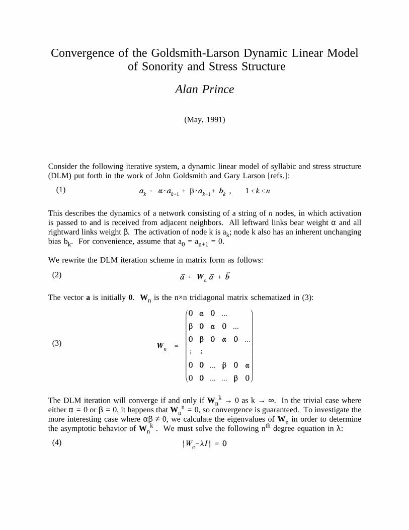
Convergence of the Goldsmith-Larson Dynamic Linear Modelof Sonority and Stress Structure

Alan Prince

(May, 1991)

Consider the following iterative system, a dynamic linear model of syllabic and stress structure(DLM) put forth in the work of John Goldsmith and Gary Larson [refs.]:

This describes the dynamics of a network consisting of a string ofn nodes, in which activation

(1)

is passed to and is received from adjacent neighbors. All leftward links bear weightα and allrightward links weightβ. The activation of node k is ak; node k also has an inherent unchangingbias bk. For convenience, assume that a0 = an+1 = 0.

We rewrite the DLM iteration scheme in matrix form as follows:

The vectora is initially 0. Wn is the n×n tridiagonal matrix schematized in (3):

(2)

The DLM iteration will converge if and only ifWnk → 0 as k→ ∞. In the trivial case where

(3)

eitherα = 0 or β = 0, it happens thatWnn = 0, so convergence is guaranteed. To investigate the

more interesting case whereαβ ≠ 0, we calculate the eigenvalues ofWn in order to determinethe asymptotic behavior ofWn

k . We must solve the following nth degree equation inλ:

(4)

The determinant Dn we need to compute looks like this:

The determinant Dn has symmetry properties which allow us to write out a recurrence formula

(5)

for it. Performing first three steps of the cofactor expansion yields the following:

Since D2 = λ² αβ, the initial conditions must be as in (7)

(6)

(7)

Recurrence relations like that in equation (6) are commonly solved in elementary number theory;observe that eq. (6) defines the Fibonacci sequence whenλ = 1 andαβ = 1. Paul Smolenskyhas provided the following perspicuous approach to deriving the solution in radicals. Observethat (6) is a homogeneous 2nd order difference equation, which can be re-written as (8):

To solve this, we start with the Ansatz (9):

(8)

Substituting this into (8) yields

(9)

(10)

50

For r≠0, this has two solutions, given by the quadratic formula:

The general solution of eq. (8) is then

(11)

Plugging this into the initial conditions (7) gives the following:

(12)

For λ² ≠ 4 αβ, we may re-arrange the last two lines of (14) to get this:

(13)

(14)

Adding to (15) the equation c1 + c2 = 1, from (13), yields this:

(15)

Since c1 + c2 = 1, we must have

(16)

(17)

51

Whence, plugging into (12),

To solve Dn = 0, let us consider those cases whereλ is real. The radical formula can be

(18)

rendered more manageable by the following substitution forλ:

The condition onΘ reflects the fact thatλ²≠ 4αβ if (18) is to make sense. The substitution (19)

(19)

allows us to explore a range of values forλ, both real (forαβ > 0) and imaginary (forαβ < 0),which will turn out to cover all the cases. The substitution yields the following:

Plugging these into (18), we find

(20)

(21)

(22)

Note that sinΘ ≠ 0. We must also assume thatαβ ≠ 0, as we have throughout.

(23)

52

To solve Dn = 0, we divide out all the irrelevant terms, obtaining

This immediately gives us:

(24)

Note that k>0 because sinΘ ≠ 0. Similarly, k ≠ n+1. Thus, we have computed n eigenvalues

(25)

λk, using eq. (19):

Since there are n distinct eigenvalues given by this formula, and since the equation we wish to

(26)

solve is of the nth degree, we conclude that all eigenvalues have been enumerated.Since the n×n matrixWn has n distinct eigenvalues, it is diagonalizable. Thus there is

a matrixQ such thatWn = QVnQ-1, with Vn diagonal. Now,Wn

m = (QVnQ-1)m = QVn

mQ-1.Thus, as m→ ∞, Wn

m → 0 iff Vnm → 0 iff λk

m → 0. Since allλk are of the simple formror ir , r ∈ , to getλk

m → 0 as m→ ∞, we must haveλk < 1. To guarantee convergence ofthe DLM iteration, then, we need

Since the cosine term is largest for k = 1 (equivalently k = n), the fraction on the r.h.s of (27)

(27)

is smallest, and we can conclude that the exact condition for convergence is therefore that givenhere:

Since the cosine term on the r.h.s. of (28), (4) is always less than 1, the entire r.h.s is always

(28)

great than ¼, for all n. We therefore arrive at the following general condition:

(29) DLM Convergence Theorem. Any Dynamic Linear Model with αβ ≤ ¼ will converge,for all n, n the number of nodes in the network.

53

54

RuCCS TR-1Part III

Closed-form Solutionof the Goldsmith-Larson Dynamic Linear

Modelof Syllable and Stress Structure

andSome Properties Thereof

Alan PrinceDepartment of Linguistics

Center for Cognitive ScienceRutgers, the State University of New Jersey

(Originally circulated June, 1991)

55

Abstract

Closed-form solution is obtained for the convergent cases of the affine iterationa ← Wna + b, whereWn is an n×ntridiagonal matrix with 0 on the main diagonal,α ∈ on the supradiagonal andβ ∈ on the subdiagonal. Thishas been proposed by Goldsmith and Larson as a key element in models of syllable structure and stress patterns.We aim to find an expression forb* = ( I W n ) 1b, which gives the fixed pointb* achieved by starting from anyb and initial conditiona = 0.

Since the function relating inputb to outputb* is linear, we examine the effect of the iteration on the canonical basisvectorsek, and develop expressions forek*. Particularly simple solutions exist for the caseαβ = ¼. Let r =(α/β)½. Then we have:

A variety of basic properties of theek* are demonstrated, under various constraints on the signs ofα andβ, includingthese:

(1) The signs of the entries inek* (ejk*) to the left of ekk* are determined entirely by the sign ofα,alternating fromekk* when α < 0. Similarly the signs of theejk* to the right ofekk* are determined entirely by thesign of β.

(2) When the signs ofαβ agree,αβ > 0, the absolute values of theejk* have one and only maximum, towhich the values rise and from which the values fall monotonically. This maximum may be shared between 2adjacent nodes. The maximum can be placed on any entryejk* in a given ek* by suitable choice of parametersαandβ.

(3) When the signs ofαβ disagree,αβ < 0, there are 3 types of behavior with respect to absolute valuesof theejk*; (i) a simple rise toekk* and fall from it; (ii) a condition in which low amplitude ripples develop, movingin from the edge toekk* over a very flat region, with a rapid fall-off beyondekk*; (iii) a uniform fall (or uniformrise) over the whole vector; i.e. maximum value at one edge or the other.

(4) The placement of maxima of absolute value, for givenα andβ, does not depend on the length of thevector (n of Wn), but is measured from an edge.

Since maximum-behavior is shown to be uniform in each of the sign-conditions, it is suggested thatαβ can be fixed,reducing the permitted range of parametric variation. Forαβ > 0, attention may be limited to the modelsαβ= ¼,which are easy to solve, and therefore deserve to be called the ‘Canonical Models’.

Part III concludes with discussion of the formal and linguistic ramifications of the results, along with a tentativeclassifications of the models. It is shown, for example, that models withαβ > 0 can be linguistically interpreted asallowing an accent to fall no further from a specified edge than syllablej, with lexical accents surfacing only whenthey fall inside this limit. Indeed, the Canonical Models can easily be parametrized directly in terms the limit.Limited attention is paid to behavior of inputs more complex thanek, that is, weighted sums ofek; but the vector(1, 1, 1, ...) = k ek is examined in the Canonical Models, withα=β=±½. This vector can be interpreted as a stringof syllables undifferentiated as to quantity. Its image under the model is shown to have a complete mirror-imagesymmetry, and, therefore, in the conditionα=β= ½, a kind of edge-in pattern of alternating maxima which, in theeven-length case, induces clashes or lapses mid-string. Various other properties are noted, and it is suggested thatlimiting the accuracy with which parameters may be set, along with a requirement that models be behaviorally stableover the range of accuracy, might lead to a resolution of some of the nonlinguistic properties of the model.

56

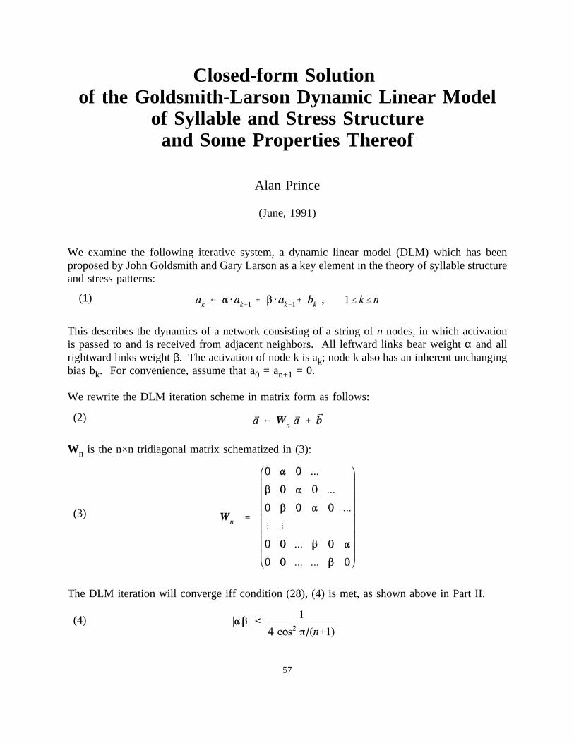
Closed-form Solutionof the Goldsmith-Larson Dynamic Linear Model

of Syllable and Stress Structureand Some Properties Thereof

Alan Prince

(June, 1991)

We examine the following iterative system, a dynamic linear model (DLM) which has beenproposed by John Goldsmith and Gary Larson as a key element in the theory of syllable structureand stress patterns:

This describes the dynamics of a network consisting of a string ofn nodes, in which activation

(1)

is passed to and is received from adjacent neighbors. All leftward links bear weightα and allrightward links weightβ. The activation of node k is ak; node k also has an inherent unchangingbias bk. For convenience, assume that a0 = an+1 = 0.

We rewrite the DLM iteration scheme in matrix form as follows:

Wn is the n×n tridiagonal matrix schematized in (3):

(2)

The DLM iteration will converge iff condition (28), (4) is met, as shown above in Part II.

(3)

(4)

57

Supposeα and β are fixed so that DLM converges. Let theb* be the result when the DLMiteration converges given a bias vectorb. The vectorb* is a fixed point of the iteration, so wehave

That is,

(5)

This yields a formula forb* in terms of b.

(6)

(7)

The form of the entries in (I W n)1 can be determined straightforwardly from a calculation on

(I W n), which looks like this:

Let Em be the determinant of (I W m). Let cjk be the generic entry in (I W n)1. We have

(8)

the following result:

(9)

Sketch of proof. These formulas are obtained by the standard inversion procedure, whereby(A 1)jk = ( 1)j+k cof(A)kj / A . The cofactor of ajk is the matrix obtained from A by omittingrow j and columnk. Two observations are required to apply this procedure to the matrix (IWn) and get the result in eq. (9).

58

First, there’s a generalization of the notion of a triangular matrix to what we might call‘block triangular’, in which the elements along the diagonal are blocks rather than single entries.Such a matrix will look, e.g., like this:

This matrix might be called ‘lower block triangular’; reflecting it through the diagonal, so that

(10)

the all-0 part lies in the lower triangle, also produces a block-triangular matrix. Just as thedeterminant of an upper or lower triangular matrix is equal to the product of its diagonalelements, so the determinant of a block-triangular matrix is equal to the product of thedeterminantsof its diagonalblocks.

Second, the cofactor of any entry ajk in (I W n) turns out to be block-triangular. Inparticular, for j≥ k cof(ajk) has one block of size (j 1)×(j 1) in the upper left-hand corner,another block of size (n k)×(n k) in the lower right-hand corner. For j≤ k cof(ajk) has oneblock of size (k 1)×(k 1) in the upper left-hand corner, another block of size (n j)×(n j) in thelower right-hand corner. If j > k, so that ajk is in the upper triangle, the all-zero part of thecofactor matrix lies in the lower triangle, and the two blocks are connected by a string ofβ’son the diagonal, (j k) of them. If j < k, so that ajk is in the lower triangle, its cofactor is lowerblock-triangular, as in ex. (10), and the two blocks are connected by a diagonal ofα’s, (k j)in number.

The formulas in eq. (9) follow immediately. The fate of the ( 1)j+k factor in the genericformula is worth tracking: it has the same sign as (α)k j and ( β)j k, so it simply disappearsfrom the calculation.

Let us evaluate the determinants in eq. (9). The expressionI W n = En has thegeneral form of the determinant evaluated previously in the process of finding the eigenvaluesof Wn. From Part II, eqs. (11) & (18), we derive, withλ = 1, this formula:

To render this more manageable, we introduce a parameteru with this definition:

(11)

Let u be complex and restricted to u = U + iΘ, where U > 0 andΘ = 0 or Θ = π/2; or U = 0

(12)

and 0 <Θ < π/(n+1). Then a uniqueu can be found for any values ofα andβ such that 4αβcosh2 u = 1.

59

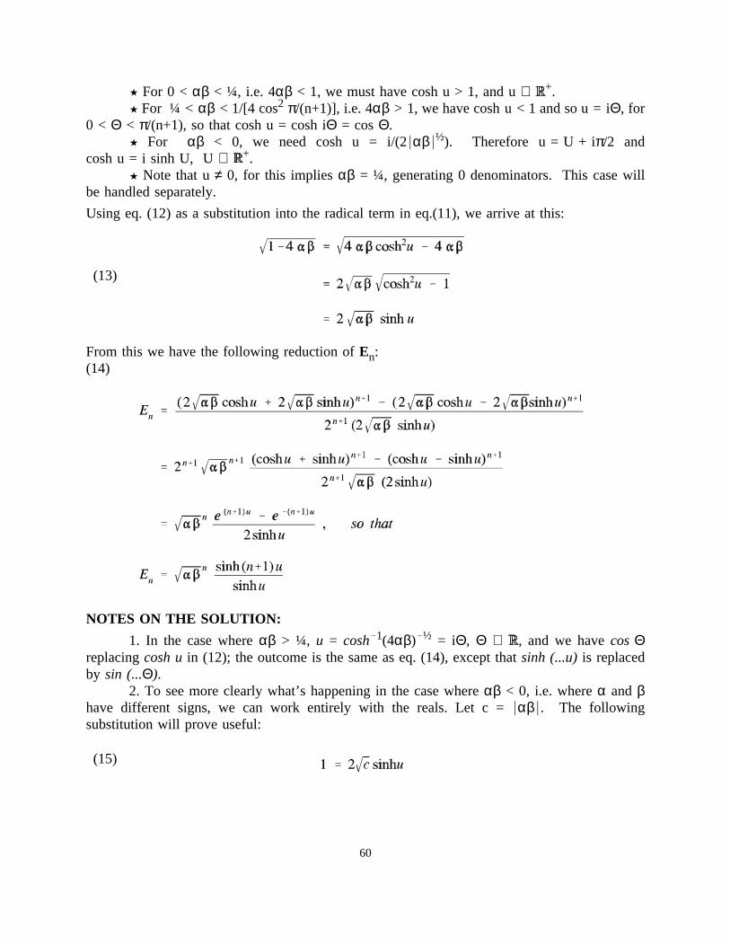
For 0 < αβ < ¼, i.e. 4αβ < 1, we must have cosh u > 1, and u∈ +.For ¼ <αβ < 1/[4 cos2 π/(n+1)], i.e. 4αβ > 1, we have cosh u < 1 and so u = iΘ, for

0 < Θ < π/(n+1), so that cosh u = cosh iΘ = cosΘ.For αβ < 0, we need cosh u = i/(2αβ ½). Therefore u = U + iπ/2 and

cosh u = isinh U, U ∈ +.Note that u≠ 0, for this impliesαβ = ¼, generating 0 denominators. This case will

be handled separately.

Using eq. (12) as a substitution into the radical term in eq.(11), we arrive at this:

From this we have the following reduction ofEn:

(13)

NOTES ON THE SOLUTION:

(14)

1. In the case whereαβ > ¼, u = cosh 1(4αβ) ½ = iΘ, Θ ∈ , and we havecosΘreplacingcosh uin (12); the outcome is the same as eq. (14), except thatsinh (...u)is replacedby sin (...Θ).

2. To see more clearly what’s happening in the case whereαβ < 0, i.e. whereα andβhave different signs, we can work entirely with the reals. Let c =αβ . The followingsubstitution will prove useful:

(15)

60

The radical term and the expressions involving it come out as follows:

Putting these into eq. (11) yields this:

(16)

(17)

(18)

(19)

END OF NOTES.

61

Since the map G:b b* given by (I W n)1 is linear, its properties are fully determined

by its effect on a basis for n. It is instructive, therefore, to calculate the mapek ek*, whereek is the canonical basis vector with 1 in the kth coordinate and 0 elsewhere. Sinceb = bkek,the behavior ofb b* in general is just the additive superimposition of individual terms of theform G(bkek) = bkG(ek) = bkek*.

In terms of the underlying network, the jth coordinate ofek*, πj(ek*), which we will writeas ejk*, represents the isolated effect on the jth node of the unit bias at the kth node, since allnodes except k have bias 0. Because of linearity, effects emanating from different node-biasesdo not interactbut merely superimpose, and once we have calculated the effect of the isolatedunit biases, in principle we have the wherewithal to learn everything about how the networkworks.

What we need to calculate, then, isek* = ( I W n)1 ek. This is simply the kth column

of (I W n)1, whose elements are described by the formulas in eq. (9). The Em’s can be

expressed in the terms given by eq. (14). Starting with j≤ k, that is, node j to the left of nodek, we arrive at the following:

We use the notation (sgn x) = 1 if x≥ 0, 1 if x < 0. Observe that the final denominator term

(20)

in no way depends onj or k; it is strictly a function ofα,β, and n, and therefore reflects aproperty of the network as a whole. We assign it a special symbol:

We arrive at the following expression forejk*:

(21)

To determine the rightward effects of a unit bias at node k, we turn our attention toejk* for

(22)

j ≥ k. Using the second equation in (9), we find

(23)

62

These formulas forejk* depend crucially on two measures of distance: from the node k, andfrom the edges of the network. They evince a division of the node string into 3 segments: thecentral stretch from j to k (or k to j), inclusive, and its flanks. The exponential term pertains tothe central segment; the sinh terms to the flanks.

The exponential term (α/β)(k j)/2 depends on thesigneddistance from node k: leftwardis positive, rightward is negative (these directions could be switched if we usedβ/α instead ofα/β). At node k this term is 1; node k is then like the origin for a simple exponential eax,where a = log(α/β)½. (The minus sign pops up because rightward is positive in the standardcoordinate system.) This term, whenαβ > 0 so that (α/β)½ is real, describes an exponentialdecay or inflation, depending on whetherα/β > 1 or α/β < 1, running smoothly from one endof ek* to the other. If we think of k as fixed and j varying, this can be made even more clearby placing (α/β)(k/2 among the constant terms at the beginning of the expression, leaving (α/β) j/2

as the exponential term.The sinh terms directly reflect the size of the flanks, where by ‘flank’ we mean a

contiguous stretch running from an edge-node to node j (node k resp.) which does not crossnode-k (node j resp.). When j < k, the j-flank runs frome1k* to ejk* and the relevant term is sinhju, as in eq. (22), which counts the number of nodes from node 1 to node j. The k-flank runsfrom enk* to ekk* and its term is sinh (n k+1)u, which counts the number of nodes fromekk*to enk*. When j > k, mirror-image-wise, the j-flank runs fromenk* to ejk*, giving rise to theterm sinh (n j+1)u; the k-flank runs frome1k* to ekk*, yielding sinh ku.

If we think of k as fixed, and vary j, the heart of the activation function for j≤ k and thefunction for j ≥ k can be resolved into the product of an exponential term and a sinh termdependent on j: sinh ju or sinh (n j+1)u. (The sinh term dependent on k is constant within eachof these two conditions.) Using the notation d#(m) to indicate the number of nodes from thedesignated boundary # to node m, we can write

But while the exponential term runs smoothly and montonically throughoutek*, the sinh

(24)

term splits into two parts at the node k. For j≤ k, we have # taken to be the beginning of thenode string, so that d#(j) = j and we are dealing with sinh ju, which runs up from sinh u to sinhk. For k ≥ j, # is the end and d#(j) = n j+1, so that we have sinh d#(j) = sinh (n j+1)u, whichruns down from sinh(n k+1)u to sinh u. Thus we have a near mirror-image pattern in the sinhterm.

63

As noted above, the formulas we have derived do not work forαβ = ¼. In that case, u= 0 and denominators vanishes. However, a limit argument easily establishes the result for thesevalues, which turns out to be of particular interest. In the case of leftward spreading from thenode with unit bias, where j≤ k, we need to ascertain

Since lim (xy) = (lim x)(lim y) if the limits exist, to evaluate expression (24), we break it into

(25)

factors that can be easily analyzed.

Putting these together, we find

(26)

(27)

(28)

(29)

64

Similarly,

(30)

For αβ = ¼, then, the equations simplify remarkably. The exponential term remains asbefore, but the sinh terms become linear. Thinking of k as fixed and j as variable, the sinh termrises as a line with slope 2(n k+1)/(n+1) from node 1 to node k, and falls as line with slope

2k/(n+1) from node k to node n. It is intuitively clear why this should be so: for 0 <αβ < ¼we have the function sinh d#(j)u term which, graphed, is concave upward; forαβ > ¼, thisbecomes sin d#(j)u, whose graph is concave downward; the straight line marks the limiting caseattained as each approaches the other.

*******

From formulas (9), (22), and (23) we can deduce the basic properties of the behavior ofthe DLM asα andβ vary. From the general formulas (9) for entries in (I - Wn)

1 we can derivethe most basic structure of theek*.

We repeat those formulas here for convenience:

It turns out that Em are positive. This can be seen from the following argument. The

(31)

eigenvalues of (I W n)1 are 1/(1 λk), λk an eigenvalue ofWn. The determinant of (I W n)

1

is equal to the product of its eigenvalues. From the eigenvalue calculation in Part II above, eq.(26), it follows that theλk come in positive, negative pairs. (For odd n,Wn also has aneigenvalue 0.) Thus the determinant of (I W n)

1 is the product of terms of the form 1/(1λk2).

Either λk is real and λk < 1, or λk = ip for real p so that 1λk2 = 1+p2. It follows that every

such term is positive, and their product is positive.

65

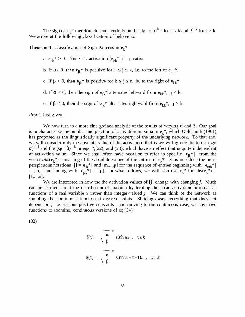
The sign ofejk* therefore depends entirely on the sign ofαk j for j < k andβj k for j > k.We arrive at the following classification of behaviors:

Theorem 1. Classification of Sign Patterns inek*

a. ekk* > 0. Node k’s activation (ekk* ) is positive.

b. If α> 0, thenejk* is positive for 1≤ j ≤ k, i.e. to the left ofekk*.

c. If β > 0, thenejk* is positive for k ≤ j ≤ n, ie. to the right ofekk*.

d. If α < 0, then the sign ofejk* alternates leftward fromekk*, j < k.

e. If β < 0, then the sign ofejk* alternates rightward fromekk*, j > k.

Proof. Just given.

We now turn to a more fine-grained analysis of the results of varyingα andβ. Our goalis to characterize the number and position of activation maxima inek*, which Goldsmith (1991)has proposed as the linguistically significant property of the underlying network. To that end,we will consider only the absolute value of the activation; that is we will ignore the terms (sgnα)k j and the (sgnβ)j k in eqs. ?,(22), and (23), which have an effect that is quite independentof activation value. Since we shall often have occasion to refer to specificejk* from thevectorabs(ek*) consisting of the absolute values of the entries in ek*, let us introduce the moreperspicuous notations [j] =ejk* and [m,...,p] for the sequence of entries beginning withemk*= [m] and ending with epk* = [p]. In what follows, we will also useek* for abs(ek*) =[1,...,n].

We are interested in how the the activation values of [j] change with changingj. Muchcan be learned about the distribution of maxima by treating the basic activation formulas asfunctions of a real variablex rather than integer-valuedj. We can think of the network assampling the continuous function at discrete points. Sluicing away everything that does notdepend onj, i.e. various positive constants , and moving to the continuous case, we have twofunctions to examine, continuous versions of eq.(24):

(32)

66

We need derivatives of these functions. For convenience,let a = log (αβ)½. First, f(x):

An extremum occurs only if

(33)

As we know from the above discussion, the function g(x) is a lightly disguised version

(34)

of f(x). Let us put it into the same form as f(x), so that conclusions drawn from analysis of theone transfer transparently to the other. Let x = n y+1; then we have

We can discard the constant part of the exponential term, as it does not affect the location of

(35)

extrema; we have, then,

The character of the solutions to these equations depends on the status ofu, which in turn

(36)

depends onαβ. There are two basic cases to consider,I. αβ > 0 andII. αβ < 0

Condition I further splits into two subcases:Ia. 0 < αβ < ¼ andIb. ¼ < αβ < [4 cos2 π/(n+1)] 1.

Let us pursue each of these in turn.

67

I. αβ > 0.

For the case ¼ >αβ > 0, general considerations based on the above discussion suggestthe following: there ought to be a single maximum inek*. The exponential term is monotonic;the sinh term rises and then falls. Suppose, for concreteness, thatα > β, so that the exponentialterm increases. The exponential term agrees in direction up to node k with the sinh term; themaximum on this segment lies at node k. On the second segment, from node k to node n, thetwo terms disagree in direction. Because of monotonicity, the interaction is rather simple,allowing for a maximum anywhere between node k and node n, depending on the parametersbut only for one such maximum. As it happens, the caseαβ > ¼ also allows only onemaximum the non-monotonicity of sin x doesn’t get enough room to play. Let us proceed tothe proof of both these assertions.

Theorem 2. Suppose 0 <αβ < ¼. There is single maximum of the absolute value of activationin ek*, for all k, 1≤k≤n . Activation rises monotonically to the maximum, and fallsmonotonically from it.

Proof. Since 0 <αβ < ¼, from 4αβ cosh2u = 1, we have 0 < u <∞. Therefore, ux > 0,both cosh and sinh are strictly increasing, and since cosh y > sinh y, for all y, it follows that eq.(34) has a solution iff a > u . This relation between a=log(α/β)½ and u=cosh1(½(αβ) ½) canalways be arranged, with proper choice ofα andβ, as can a≤ u. To evaluate the character ofthe extremum, we examine f″(x):

(37)

But at f′(x) = 0 we have cosh ux = (a/u) sinh ux, so this comes out as

Since a>u when f′(x) = 0, it follows that f″(x) < 0 at such points. Therefore, all points where

(38)

f′(x) =0 are maxima. Since f′(x) = 0 has exactly one solution when a > u, and none otherwise,f(x) has one and only maximum and that occurs iff a > u. Furthermore, since f′(x) > 0 beforethe maximum and f′(x) < 0 after it, it follows that f is monotonic up to the maximum andmonotonic down from the maximum. For a≤ u, f is monotonic increasing.

Similar remarks apply to g(x). From the direct parallel between h(x) and f(x) we have,immediately, that there is a maximum iff b > u and none iff b≤ u. If b ≤ u, then h(y) ismonotonic increasing, but g(x) monotonically decreasing, because x = n y+1. Since b = a, wehave the following relations between f(x) and g(x):

i) If a> u > 0 > b , then f has a maximum;g decreases.ii) If u ≥ a and u≥ b , thenf increases;g decreases.iii) I f b > u > 0 > a,theng has a maximum;f increases.

68

These results apply to f(x) and g(x) without regard for limitations on the domain of x.Application to the circumscribed domains 1≤ x≤ k and k≤ x ≤ n is, however, straightforward.

i) Suppose a>u>0>b. The function f has a maximum. If it occurs for x < 0, then [1] bearsthe maximum inek*. If it occurs for x > k, then [k] bears the maximum. Otherwise themaximum occurs on [j] =ejk*, for 1 ≤ j ≤ k. Note that activation falls from [k] to [n], since gis decreasing. Note also that since [k] belongs to both spans, we can conclude that everythingin [k,...,n] to the right of k is less than anything in [1,...,k].

ii) Suppose u≥a and u≥b. Then f increases and g decreases. Therefore [k] bears themaximum.

iii) Suppose b>u>0>a. This is just the mirror image of case (i). The maximum falls on[j], k ≤j ≤n.

Let us turn to the case ¼ <αβ < [4 cos2 π/(n+1)] 1. We have u = iΘ, so that coshu = cosΘ, and sinhu = i sin Θ, where 0 <Θ < π/(n+1). (The i divides out, ensuring a realanswer for [j].) The term sinΘj in the activation function therefore ranges over the interval 0< Θj < nπ/(n + 1). The appearance of the sinΘj, which is not monotonic on the interval underconsideration, suggests that new behaviors might arise, but no such untoward event happens.Potential maxima in [1,...,k] are located by solving the equation below, paralleling eq. (34):

(39)

This has a unique solution for any legitimate choice of a=log(αβ)½ andΘ = cos 1(4αβ) ½, namely x =Θ 1 cot 1(a/Θ), where 0 < cot 1φ < π. Furthermore, it is clearthat the expression on the l.h.s starts out positive, turns 0, then remains negative: (Θ cosΘx)starts out at (arbitrarily near)Θ>0, and runs down to (arbitrarily near)Θ, while (a sinΘx) startsout at (arbitrarily near) 0 and ends up back at (arbitrarily near) 0. These lines must cross. Thusthe zero of the first derivative is at amaximum, to which the activation function risesmonotonically and from which it falls monotonically.

69

Correspondingly, a maximum for the function g related to the case j≥k is guaranteed bythe parallel equation withb=log (β/α)½ in place ofa, and y = n x+1 in place of x. Here wehave y =Θ 1 cot 1(b/Θ). Since cot1( φ) = π cot 1(φ), and since b = a, we can derive thefollowing relation between the solution for j≤ k(call it xf) and the solution for j≥ k (call it xg):

Noting thatπ/(n+1) > Θ, i.e. thatπ/Θ > n+1, we conclude that xg < xf. This means that the

(40)

maximum for g(x) occursto the leftof the maximum for f(x). This will lead us immediately tothe following strengthened version of Thm. 2:

Theorem 3. Let α andβ be chosen so that the DLM converges. Supposeαβ > 0. There is singlemaximum of the absolute value of activation inek*, for all k, 1 ≤ k ≤ n . Activation risesmonotonically to the maximum, and falls monotonically from it.

Proof. Theorem 2 establishes the result forαβ < ¼. Two cases remain:αβ > ¼ andαβ = ¼.Let us begin withαβ > ¼.

We know that each activation function has a maximum. We need to show that,nevertheless,ek* = [1,...,n] has only one local maximum. Suppose that the left hemi-network[1,...,k] has a maximum on [j], 1≤j<k. Now we know from the above remarks that the maximumof the continuous activation functiong for the right hemi-network [k,...,n] occursbeforex = j.. Sinceg decreases after its maximum, it follows that activation decreases from [k] to [n].

70

Suppose now that the maximum for the left hemi-network [1,...,k] falls on [k]. In termsof the corresponding continuous activation function f(x) this is ambiguous between two cases:(i) f has a maximum at some x near k, which would entail that [k] is a left maximum; and (ii)the maximum for f(x) is somewhere off to the right, so that f(x) is rising toward it when it is cutoff, as it were by node k. In case (i), g(x) has its maximum on or before x = k, [k] is themaximal node in the whole network. In case (ii), g(x) can have its maximum anywhere fromx=k to x=n, depending on how far to the right the maximum of f(x) falls, and the maximum ofek* will fall in [k,...,n]. This covers all cases forαβ > ¼.

Now, to conclude, we must consider what happens whenαβ = ¼. The relevant continousactivation function and its derivatives are as follows:

When f′(x) = 0, we have

(41)

Notice that the sign of f″(x) depends on the sign of a = log(α/β)½. For this case, then,

(42)

f has both maxima and minima, depending on theα,β parameter settings, so long as a≠ 0: forα>β, there is a maximum at x = 1/a; forα<β, there is a minimum at x = 1/a = 1/a and noother extrema. Of course, in the discrete system we are modeling, there are only positive-numbered nodes. Thus, forα/β > 1, the left hemi-network [1,...,k] has a maximum [j], 1≤ j ≤k. For α/β < 1, activation increases monotonically, and [k] bears the maximum. Parallelconsiderations apply in the usual mirror-image form to the right hemi-network [k,...,n]. Thus,when α/β > 1, so thatβ/α < 1, there is falling activation from node k to node n; the wholenetwork’s maximum then falls in [1,...,k]. Whenα/β < 1, so thatβ/α > 1, the network’smaximum falls in the right hemi-network [k,...,n]. Whenα = β, a = log(α/β)½ = 0, and f(x) risesto infinity on a straight line, g(x) falls the same way, and [k] bears the maximum, which is2k(n k+1)/(n+1), by direct computation.

71

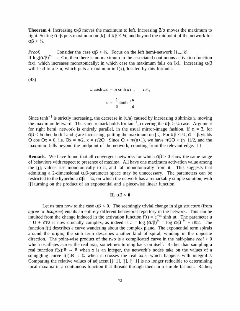
Theorem 4. Increasingα/β moves the maximum to left. Increasingβ/α moves the maximum toright. Settingα=β puts maximum on [k] ifαβ ≤ ¼, and beyond the midpoint of the network forαβ > ¼.

Proof. Consider the caseαβ < ¼. Focus on the left hemi-network [1,...,k].If log(α/β)½ = a ≤ u, then there is no maximum in the associated continuous activation functionf(x), which increases monotonically; in which case the maximum falls on [k]. Increasingα/βwill lead to a > u,which puts a maximum in f(x), located by this formula:

Since tanh1 is strictly increasing, the decrease in (u/a) caused by increasinga shrinksx, moving

(43)

the maximum leftward. The same remark holds for tan1, covering theαβ > ¼ case. Argumentfor right hemi network is entirely parallel, in the usual mirror-image fashion. Ifα = β, forαβ < ¼ then both f and g are increasing, putting the maximum on [k]. Forαβ < ¼, α = β yieldsΘ cosΘx = 0, i.e.Θx = π/2, x = π/2Θ. SinceΘ < π/(n+1), we haveπ/2Θ > (n+1)/2, and themaximum falls beyond the midpoint of the network, counting from the relevant edge.

Remark. We have found that all convergent networks for whichαβ > 0 show the same rangeof behaviors with respect to presence of maxima. All have one maximum activation value amongthe [j]; values rise monotonically to it, and fall monotonically from it. This suggests thatadmitting a 2-dimensionalα,β-parameter space may be unnecessary. The parameters can berestricted to the hyperbolaαβ = ¼, on which the network has a remarkably simple solution, with[j] turning on the product of an exponential and a piecewise linear function.

II. αβ < 0

Let us turn now to the caseαβ < 0. The seemingly trivial change in sign structure (fromagreeto disagree) entails an entirely different behavioral repertory in the network. This can beintuited from the change induced in the activation function f(t) = eat sinh ut. The parameter u= U + iπ/2 is now crucially complex, as indeed is a = log (α/β)½ = log α/β ½ + iπ/2. Thefunction f(t) describes a curve wandering about the complex plane. The exponential term spiralsaround the origin; the sinh term describes another kind of spiral, winding in the oppositedirection. The point-wise product of the two is a complicated curve in the half-planereal > 0which oscillates across the real axis, sometimes turning back on itself. Rather than sampling areal function f(x): → when x is an integer, the network’s nodes take on the values of asquiggling curve f(t): → when it crosses the real axis, which happens with integralt.Comparing the relative values of adjacent [j 1], [j], [j+1] is no longer reducible to determininglocal maxima in a continuous function that threads through them in a simple fashion. Rather,

72

between each pair of node values the associated continuous function loops off into the complexplane and comes back. Consequently, the localistic methods used above are not applicable.Instead, we must directly compare [j] and its neighbors. It turns out to be informative (ultimatelyindeed, more precisely informative than the continuous methods can be) to examine theratiobetween [j] and its immediate neighbors. When [j]/[j 1] > 1 and [j]/[j+1] > 1, we have amaximum at [j].

As a preliminary to the analysis, it is useful to cash in the product of the two complexterms for their real value. For the exponential term, we have

The sinh term becomes

(44)

The trigonometric terms take on the values {0,1, 1} for integralj, while the term ( i)j cycles

(45)

among the values {1, i, 1, i}. Their product ends up real, and alternates between sinh Uj, forj even, and cosh Uj, j odd, as can be seen from the following table:

j ( i) j sinh uj ( i)j sinh uj

4m 1 sinh Uj sinh Uj4m+1 i i cosh Uj cosh Uj4m+2 1 sinh Uj sinh Uj4m+3 i i cosh Uj cosh Uj

We must therefore consider different functions, depending on whether j is even or odd. Writefjk* for [j] = ejk* with all j-free factors divided out, and let r =α/β ½ :

(46)

73

We want to establish the following characterization of the structure of [1,...,k] as the parametersvary:

1. For α <1, [j] rises monotonically to [k], 1≤j≤k.2. For α > 1/(1 β ), activation falls monotonically from [1] to [k].3. For 1 < α < (1 β ) 1, as α increases, a low-amplitude alternating ripple with

maxima on [j], j even, and minima on [j],j odd, j < k, spreads from [1] to [k].The usual mirror-imaging remarks apply to [k,...,n].

Let us now establish a series of assertions that will lead to this characterization. In whatfollows, we assumeαβ < 0. Recall that we are abstracting away from sign alternations and bythe symbol [j] we always mean theabsolute valueof the activation of node j. When discussingthe network segment [1,...,k] we mean by ‘maximum on [j]’ that [j] > [j 1] and [j] > [j+1], for1<j<k; when j=1, we mean only [1] > [2], and when j=k, we mean only [k] > [k 1]. Similarremarks hold for the segment [k,...,n]. It will be useful to introduce the term ‘quasi-maximumon [j]’, by which we mean [j]≥ [j 1] and [j] ≥ [j+1]. All discussion will be centered on the lefthemi-network [1,...,k], since conclusions about it can be immediately converted into conclusionsabout [k,...,n].

Lemma 1. No quasi-maximum occurs on any [j], j≠k, in [1,...,k], if j is even.

Proof. For a quasi-maximum to sit on [j], j even, we must have

But these conditions can never hold simultaneously. The reason is that

(47)

(48)

(49)

74

To establish this, we invoke the following identity, which is easily verified from the definitionof sinh x:

We have, therefore,

(50)

Since this last is self-evident, we follow the implicit chain ofiff’s back up to conclude that

(51)

inequality (49) is sound.

Corollary . There is a choice ofα, β such that a minimum or quasi-minimum can be placed onany even [j] in [1,...,k].

Proof. This follows immediately from inequality (49); an r can always be chosen that fitsbetween l.h.s and r.h.s.

Lemma 2. There is a choice ofα,β such that a maximum or quasi-maximum can be placed onany [j], j odd, in [1,...,k].

Proof. This follows from a calculation analogous to the one just performed, with sinh and coshswapped, due to the change in parity of j. To put a maximum or quasi-maximum on [j], j odd,we must have

There will always be such an r if the far l.h.s is always greater than the far r.h.s., which indeed

(52)

it is. To show this, we need only establish:

(53)

But cosh u > sinh u , u∈ , so that cosh2 mx > sinh2 mx, and sinh2mx > sinh(m+1)xsinh(m 1)x, by identity (50). Observe that the strictness of inequality (53) entails that we cannever have [j 1] = [j] = [j+1].

75

Lemma 3. Even-Odd Rule. If [j 1] ≤ [j] , for some odd j, then [m 1] < [m] for all precedingodd m < j. That is, if we pick r so that there is equality or rise over an even-odd nodesequence, then there is a rise over every preceding even-odd sequence.

Equivalently, by contraposition, if [m 1]≥ [m] for odd m, then [j 1] > [j], m < j, j odd.That is, if there is equality or fall over an even-odd node sequence, then all following even-oddsequences are strictly falling.

Proof. If the assumption holds, then we have:

We need to show that r satisfies the analogous inequality for all preceding odd m < k. This will

(54)

happen if

This relation holds if F(x) = (cosh ux)/sinh u(x 1) decreases strictly with increasing x; which it

(55)

does, because sinh plays steady catch-up with cosh. More formally,

Since this is always negative when defined (x≠ 1), F(x) is strictly decreasing in the interval

(56)

we’re interested in.

76

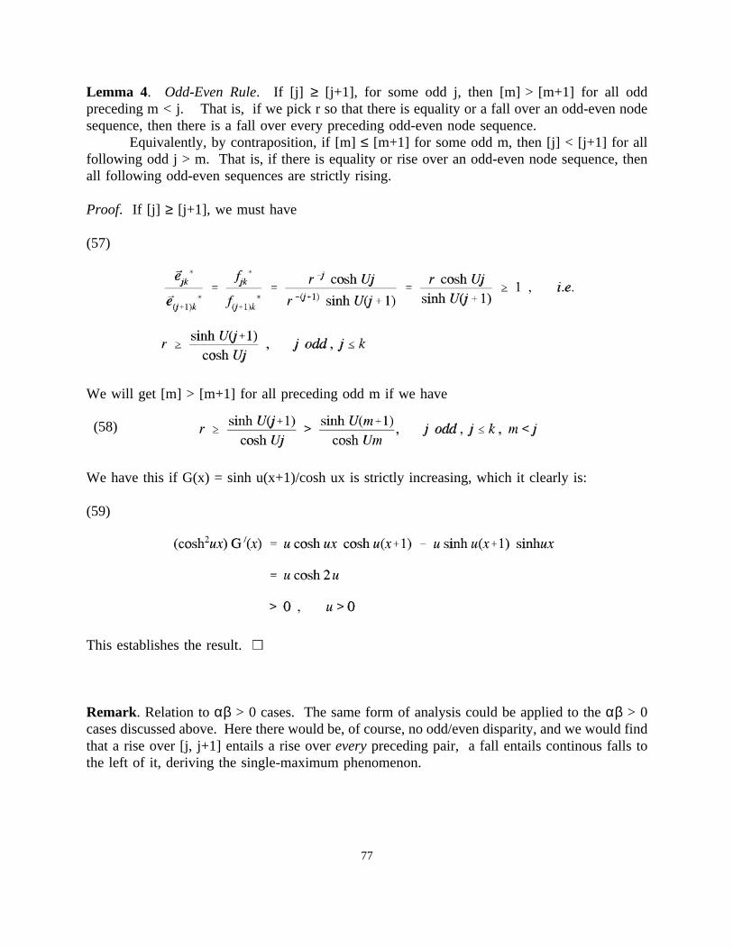
Lemma 4. Odd-Even Rule. If [j] ≥ [j+1], for some odd j, then [m] > [m+1] for all oddpreceding m < j. That is, if we pick r so that there is equality or a fall over an odd-even nodesequence, then there is a fall over every preceding odd-even node sequence.

Equivalently, by contraposition, if [m]≤ [m+1] for some odd m, then [j] < [j+1] for allfollowing odd j > m. That is, if there is equality or rise over an odd-even node sequence, thenall following odd-even sequences are strictly rising.

Proof. If [j] ≥ [j+1], we must have

We will get [m] > [m+1] for all preceding odd m if we have

(57)

We have this if G(x) = sinh u(x+1)/cosh ux is strictly increasing, which it clearly is:

(58)

This establishes the result.

(59)

Remark. Relation toαβ > 0 cases. The same form of analysis could be applied to theαβ > 0cases discussed above. Here there would be, of course, no odd/even disparity, and we would findthat a rise over [j, j+1] entails a rise overeverypreceding pair, a fall entails continous falls tothe left of it, deriving the single-maximum phenomenon.

77

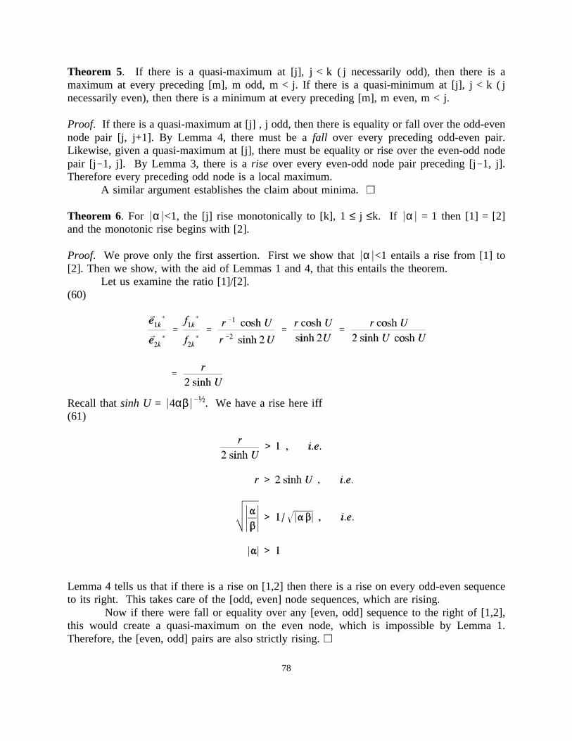
Theorem 5. If there is a quasi-maximum at [j], j < k ( j necessarily odd), then there is amaximum at every preceding [m], m odd, m < j. If there is a quasi-minimum at [j], j < k ( jnecessarily even), then there is a minimum at every preceding [m], m even, m < j.

Proof. If there is a quasi-maximum at [j] , j odd, then there is equality or fall over the odd-evennode pair [j, j+1]. By Lemma 4, there must be afall over every preceding odd-even pair.Likewise, given a quasi-maximum at [j], there must be equality or rise over the even-odd nodepair [j 1, j]. By Lemma 3, there is arise over every even-odd node pair preceding [j 1, j].Therefore every preceding odd node is a local maximum.

A similar argument establishes the claim about minima.

Theorem 6. For α <1, the [j] rise monotonically to [k], 1≤ j ≤k. If α = 1 then [1] = [2]and the monotonic rise begins with [2].

Proof. We prove only the first assertion. First we show thatα <1 entails a rise from [1] to[2]. Then we show, with the aid of Lemmas 1 and 4, that this entails the theorem.

Let us examine the ratio [1]/[2].

Recall thatsinh U = 4αβ ½. We have a rise here iff

(60)

Lemma 4 tells us that if there is a rise on [1,2] then there is a rise on every odd-even sequence

(61)

to its right. This takes care of the [odd, even] node sequences, which are rising.Now if there were fall or equality over any [even, odd] sequence to the right of [1,2],

this would create a quasi-maximum on the even node, which is impossible by Lemma 1.Therefore, the [even, odd] pairs are also strictly rising.

78

Theorem 7. For α > 1/(1 β ), the [j] fall monotonically from [1] to [k], 1≤ j ≤ k.

Proof. First we show that the condition onα entails a fall over node-pair [2,3]. Then we show,with the aid of Lemmas 1 and 3 that this entails a fall throughout the segment [1,....,k].

Since β >0, we have α > 1. Therefore there is a fall over [1,2] which continues over [2,3].

(62)

The fall on [2,3] entails, by Lemma 3, a fall over every [even, odd] pair to its right. This takescare of [even,odd].

Now suppose that there is equality or rise over [odd, even]. Since we have shown that[even, odd] is always falling, this would force a quasi-maximum on an even node, animpossibility by Lemma 1.

We have thus far described the situation in static, implicational terms. The method we have usedto derive these descriptions, however, has also given us sufficient information to put together apicture of how network behavior changes as r =αβ ½ changes.

Theorem 8. As r = αβ ½ increases, [1,...,k] is first monotonically increasing, forα < 1.For 1 < α < 1 β , as r increases, first a ripple of minima on even-numbered nodesspreads from node 2 rightward up to the last even-numbered node before k. Then a uniformlyfalling ramp spreads back from k until, forα > (1 β ) 1, the hemi-network [1,...,k]becomes monotonically decreasing.

79

Proof. We know from the proof of Lemma 3 that a node sequence [even, odd], which we canwrite as [2p, 2p+1], shows equality or rise just in case

Conversely, the sequence [even, odd] shows equality or fall when

(63)

Let’s symbolize the ratio term asC(2p,2p+1).

(64)

We know from the proof of Lemma 4 that a node sequence [odd, even] shows equalityor fall just in case

Conversely, the sequence [odd, even] shows equality or rise when

(65)

Let’s symbolize the ratio term here asS(2p 1,2p).

(66)

From the proofs of Lemma 3 and Lemma 4 we also know thatC(x,x+1) is a strictlydecreasing function; thatS(x 1,x) is strictly increasing; from the proof of Lemma 1 and Lemma2 we know thatS(x 1,x) < C(x,x+1) andS(x+1,x+2) <C(x,x+1). This gives us the followingstrict order:

Odd k:S(1,2) < S(3,4) <...<S(k 2,k 1) < C(k 1,k) <...<C(4,5) < C(2,3)

Even k:S(1,2) < S(3,4) <...<S(k 1,k) < C(k 2,k 1) <...<C(4,5) < C(2,3)

We can tabulate the effect the r-C-S relations as follows:

a. r < S(j 1,j) OE rise over [j 1,j]b. r > S(j 1,j) OE fall over [j 1,j]c. r < C(j,j+1) EO rise over [j,j+1]d. r > C(j,j+1) EO fall over [j,j+1]

With these in hand, it’s easy to see what happens asr increases. Ifr < S(1,2), thenr is less thaneverything, and monotonic increase must occur (cases a,c).

80

Whenr = S(j, j+1) we have [j]=[j+1]. Whenr > S(j, j+1) we get a fall from [j] to [j+1],occasioning a minimum at [j+1] (case b). We also retain the falls [m, m+1], m < j, that havebeen occasioned byr passingS(m, m+1). In this way, a ripple of minima (and concomitantmaxima) spreads rightward from node 1 asr increases, coming to a halt on the last even nodebefore k, which we can callevk.

As r rises past the last of theS’s, we will get r = C(evk, evk+1), inducing[evk] = [evk+1] where previously we had [evk] < [evk+1)]. With r > C(evk, evk+1), we now geta fall over [ev(k), ev(k)+1)] (case b). Recall that all [odd even] pairs are already falling. Thus,a uniformly falling ramp is extended from [k] back to [1] asr increases, until the whole of[1,...,k] is monotonically decreasing.

To complete our basic description ofek* in the conditionαβ < 0, we need to integratethe behavior of the left and right hemi-networks [1,...,k] and [k,...,n].

1. α ≥ 1. Then β <1 since αβ < ¼. The left hemi-network shows oscillatory orfalling behavior, the right side drops off (rapidly).

2. α < 1. If we haveβ <1 too, then [k] is king, and both rise to it.3. α < 1 and β ≥ 1. Then the right side rises or oscillates, and the left hemi-network

falls off (rapidly).

We return below (‘‘Discussion,’’ p. 88 ) to characterization of the gross behavior of the modelin the αβ < 0 condition, noting the following three points:

a. the narrow range of oscillatory behavior.b. the tiny amplitude of oscillationsc. the extreme flatness of activation in oscillatory interval.α ≈ 1, β ≈ α-1.

*******To conclude the overall discussion, we examine the occurence and properties of absolute

equality between neighboring nodes, under any and all conditions of convergence. This has beenexplicitly dealt with in the treatment of the caseαβ < 0, and finessed in the caseαβ > 0. Herewe assault the problem directly.

Theorem 9. Any pair of adjacent nodes inek* can be made exactly equal by appropriate choiceof parametersα andβ.

Proof. We are looking for [j] = [j+1]. Suppose j < k. From eq. (22), we want(67)

81

Dividing out the common material leaves this:

Recall thatu is a function ofαβ. But since α/β ½ can be any positive number whatever, no

(68)

matter what the value ofαβ is fixed at, this equation can always be satisfied.

Similarly, if j ≥ k,

As above, such aβ/α ½ can be always be found.

(69)

An interesting special case arises at either edge.Corollary .

When α = 1, then [1] = [2], if k ≠ 1. That is, the first two nodes have equalactivation in allek* excepte1*.

When β = 1, then [n] = [n 1] if k≠ n. That is, the last two nodes have equal activationin all ek* excepten*.

Proof. Assume k > 1.Then we have

A similar argument applies to the mirror-image case k < n.

(70)

82

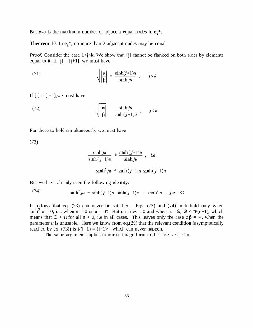
But two is the maximum number of adjacent equal nodes inek*.

Theorem 10. In ek*, no more than 2 adjacent nodes may be equal.

Proof. Consider the case 1<j<k. We show that [j] cannot be flanked on both sides by elementsequal to it. If [j] = [j+1], we must have

If [j] = [j 1],we must have

(71)

For these to hold simultaneously we must have

(72)

But we have already seen the following identity:

(73)

It follows that eq. (73) can never be satisfied. Eqs. (73) and (74) both hold only when

(74)

sinh2 u = 0, i.e. when u = 0 or u = iπ. But u is never 0 and when u=iΘ, Θ < π/(n+1), whichmeans thatΘ < π for all n > 0, i.e in all cases. This leaves only the caseαβ = ¼, when theparameteru is unusable. Here we know from eq.(29) that the relevant condition (asymptoticallyreached by eq. (73)) is j/(j 1) = (j+1)/j, which can never happen.

The same argument applies in mirror-image form to the case k < j < n.

83

Suppose now j=k. We must examine the conditions(75)

Taken together these require

(76)

This is clearly impossible for u∈ , sincesinh is strictly increasing for real arguments. Note as

(77)

u → 0, this becomes (k 1)/k = (n k+1)/(n k), which requires n=0 and so has no relevantsolutions . In the general setting, u∈ , we call on the following identity, a generalized form ofthe one cited above:

(78)

84

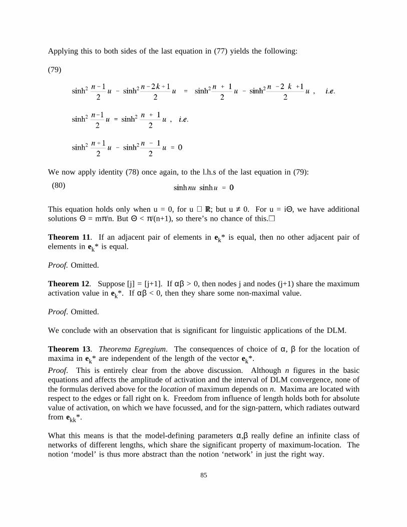
Applying this to both sides of the last equation in (77) yields the following:

We now apply identity (78) once again, to the l.h.s of the last equation in (79):

(79)

This equation holds only when u = 0, for u∈ ; but u ≠ 0. For u = iΘ, we have additional

(80)

solutionsΘ = mπ/n. But Θ < π/(n+1), so there’s no chance of this.

Theorem 11. If an adjacent pair of elements inek* is equal, then no other adjacent pair ofelements inek* is equal.

Proof. Omitted.

Theorem 12. Suppose [j] = [j+1]. Ifαβ > 0, then nodes j and nodes (j+1) share the maximumactivation value inek*. If αβ < 0, then they share some non-maximal value.

Proof. Omitted.

We conclude with an observation that is significant for linguistic applications of the DLM.

Theorem 13. Theorema Egregium. The consequences of choice ofα, β for the location ofmaxima inek* are independent of the length of the vectorek*.

Proof. This is entirely clear from the above discussion. Althoughn figures in the basicequations and affects the amplitude of activation and the interval of DLM convergence, none ofthe formulas derived above for thelocationof maximum depends onn. Maxima are located withrespect to the edges or fall right on k. Freedom from influence of length holds both for absolutevalue of activation, on which we have focussed, and for the sign-pattern, which radiates outwardfrom ekk*.

What this means is that the model-defining parametersα,β really define an infinite class ofnetworks of different lengths, which share the significant property of maximum-location. Thenotion ‘model’ is thus more abstract than the notion ‘network’ in just the right way.

85

Remarks on the Canonical Models and their Relatives.

Here we examine some significant properties of the casesαβ = ¼, which because of thesimplicity of their solution deserve to be called the ‘Canonical Models’. These properties areshared by its relatives in the classαβ > 0, and recognizing them can give insight into the entireclass. The Canonical Models has two free parameters:

(i) the sign parameter:α,β > 0, or α,β < 0, and(ii) the left-right asymmetry parameter determined by the ratioα/β, which enters

into the solution asr = α/β ½.

We will find that parameter (ii) can be readily reinterpreted to refer directly to the node-string rather than to a low-level property of the model.

The ratioα/β can be chosen put a maximum anywhere on a givenek*. For example, astraightforward calculation on the Canonical Models shows that forr = α/β ½ chosen to meetthe following restriction

a maximum will be placed on [j] inek*, if j ≤ k. (For j ≥ k, the maximum falls on [k].)

(81)

From (42), we know that a maximum fallsexactlyon node j, j≤ k, when

This equation can be solved forα (or β, or r) in terms ofj. This is the result:

(82)

This means that the Canonical Models can easily be parametrized in terms of thenodeon which

(83)

it places the maximum in the basis vectorsek*. (This is true for the other models as well, butthe translation between maximal node andr is not attractive.)

Models for whichαβ > 0 can be classified in terms of the sole maximum-node and theedge from which it is calculated. Let us say that we have the j-Model whenr is chosen so thata maximum occurs on [j] inek* if j ≤ k, and on [k] otherwise. Let us say that we have the ( j)-Model whenr is chosen so the maximum occurs on [n j+1] when j≥ k and on [k] otherwise.In the Canonical ( j)-Model this happens with r = e1/j. This classification calls on two notions:the distance from an edge to the where the maximum wants to sit; and the choice of edge.

86

Whenα = β so thatr = 1 and logr = 0, a special condition prevails, since the associatedcontinuous activation functions are monotonic: the maximum is not fixed with respect to anedge, but sits on [k] inek*, whatever k may be. Let us call these the A-Models.

It is informative to examine how a particular choice ofr affects the ensemble ofek*’s.To this end, let us contemplate a linguistic interpretation of the model. Think of theek*’s asrepresenting wordsqua syllable strings (which in fact needn’t be all of the same length wereally need another subscript to indicate the dimension of the vector; we could write, say,mekfor the kth canonical basis vector ofm; but let us put off such refinements). The unit bias inek can be taken to represent a lexical accent on the kth syllable; all other syllables areunaccented. The vectorek* is the result of processingek through DLM the phonology. Notethat every lexical word is assumed to bear one and only accent.

Suppose we want the canonical 3-Model;r = e1/3, from eq.(83). This means thecontinuous activation function f(x) associated with the initial hemi-network [1,...,k] rises to amaximum at x = 3 and falls therefrom. The corresponding activation function g(x) for the finalhemi-network [k,...,n] is falling throughout. What becomes of the variousek under this regime?The vectore1, representing initial lexical accent, has only the degenerate initial hemi-network [1],which therefore gets the maximum ine1*. The vectore2 intercepts the rise of f(x) at [2]; sinceg(x) falls thereafter, [2] bears the maximum ine2* . The vectore3* bears its maximum on [3].So do all other vectorsek* for k > 3, which host a rise to [3] and fall from it inside the initialhemi-network [1,...,k]. The situation boils down to this: lexical accents on or before node 3 winout, and carry the activation maximum, but after node 3 the lexical accent has no tropism for themaximum, which falls only on [3].

The 3-Model, then, has a kind of barrier at node 3. If the bias inek lies beyond thebarrier, it will only have the effect of supplying a reservoir of activation that pumps themaximum on [k]. But any bias which lies before the barrier,i.e. in [1,...,j] for the j-Model,gather the maximum to itself. The ( 3)-Model, of course, shows the same behavior in mirror-image, counting from the end instead of the beginning.

We find, then, two broad classes of models, the A(ccenting)-Models and the B(arrier)-Models, where the latter fall into j-Models and ( j)-Models, depending on which edge is countedfrom. For the Canonical Models, the internal parameters of the networks associated with the±j-Models can be easily determined from ±j itself.

87

Discussion

FORMAL. The findings reported here suggest certain reformulations of the model.

First, if the updating rule is modified to depend on theaverageof incoming activationrather than the simple sum, a number of cluttering factors of 2 and 4 will disappear from thebasic equations. The new rule would look like this:

Or, in matrix form:

(84)

This is equivalent to replacing Goldsmith-Larsonα, β with α/2, β/2. This done, we find that the

(85)

DLM converges iff

The parameteru is now subject to this condition:

(86)

Furthermore, the simple model found foru → 0 is now defined by the conditionαβ = 1.

(87)

A second observation is thatα and β appear in the solution principally in thecombinationsαβ andα/β (or β/α). This suggests that the basic parameters of themodelshouldbe conceived in terms of these combinations, with low-level network parametersα andβ definedfrom these more basic elements.

Suppose we identify two parameters:r, a positive quantity measuring left-rightasymmetry, andc, a quantity measuring the absolute magnitude of the activation. The followingwould provide one fairly natural correspondence with the familiarα, β:

(88)

88

Now α andβ have the following definitions:

Sincer andc are positive by stipulation, we need to add another element to the activation

(89)

rule to incorporate the possibility of sign-alternation . LetσR = ±1 be the sign attached to theactivation coming in from the right, sgn(α); let σL = ±1 be the sign attached to activation comingin from the left, sgn(β). The iteration rule now becomes:

The solutions for the Canonical Models c2 = 1 now become

(90)

The parameteru meets the conditionc2 cosh2 u = σRσL and the DLM converges when

(91)

c < secπ/(n+1). Another plausible candidate for re-parametrization would take c2 = 1/ αβ .We could also contemplate going whole-hog and defineα andβ in terms of the parametersa andu which are central to the maxima-locating equations.

*******

LINGUISTIC. A variety of linguistically promising characteristics of the DLM have been discussedby Goldsmith (1991). The patterns of sign-alternation are obviously relevant to the model’saccount of alternating stress patterns; and the single maximum phenomenon can be equated withPragueanculminationin stress or accent patterns.

Here we will mention several features of the model which emerge from the kind ofanalysis attempted in this paper. The goal is not to provide a tendentious catalogue of themodel’s deficiencies and excellences, but modestly to advance discussion of its properties. Someof these will, of course, call out for further explication, and occasional suggestions will beoffered.

89

1. Maxima. We have seen that for the modelsαβ > 0, the parameters can be chosen puta maximum (more accurately, a barrier) anywhere inek*, measuring from the edges, or to placea maximum on [k] inek*

This finding has attractive characteristics.

(i) As noted above, Theorem 13, it is independent of n, the length of the string, animportant result since string-length figures into the basic equations but not into principles oflinguistic form.

(ii) Barrier-placement allows us to model a situation roughly like that seen in a numberof accent and stress systems, whereby an accent or stress falls as far from an edge as it can, butno farther than some finite measure, usually three syllables (grossly speaking), with speciallexical accents inside the barrier nevertheless being given priority.

However, a couple of remarks:

(i) The linguist’s eye will struck by the fact thatj can be any number, rather than just thefew small ones (1, 2, 1+2) familiar from work on prosody. How can this locality property beobtained in a continuous model with an infinite parameter space? Although one might think thatthe model’s parameters will have to be limited ad hoc to a narrow zone, there may well be amore natural approach. In the Canonical Models, for example, we are guaranteed a barrier onnode j when for r = (αβ)½ we have j/(j 1) >r > (j+1)/j. This divides up range ofr in thefollowing way:

Model # r Range Length

1-Model (∞, 2) ∞2-Model (2, 3/2) 1/23-Model (3/2, 4/3) 1/64-Model (4/3, 5/4) 1/12j-Model (j/j-1, j+1/j) 1/j(j-1)

The range ofr’s that will produce thej-Model narrows rapidly asj increases. (Indeed, it narrowsvery much more rapidly in the noncanonical models, where the length of the range for puttinga maximum onj is 1/(sinh j)(sinh j 1), which falls off exponentially as opposed to quadratically.)This suggests that we can get the locality result by limiting theaccuracywith which parameterscan be set. Suppose, for example, thatr can be specified with no greater accuracy that ±.1.Putting r = 3, say, guarantees a 1-Model, becauser will range from 3.1 to 2.9. Puttingr = 1.8similarly guarantees a 2-Model. But since the interval for 3-Models is less that .17 wide, thereis no choice within it that ensures stability of the model, ifr is allowed to wander over a rangeof .2. A requirement that attained models must be stable, taken with a limitation on accuracyof parameter specification, can give a locality result.

90

The calculation for the ( j)-Models is similar, but shows an interesting shift, because ofthe wayr is defined:

Model # r Range Length

1 (0, 1/2) 1/22 (1/2, 2/3 1/63 (2/3, 3/4) 1/124 (3/4, 4/5) 1/20j (j-1/j, j/j+1) 1/j(j+1)

Where the j-Models deal withr, the ( j)-Models deal with1/r. An accuracy of .1, which wouldallow stable 1- and 2-Models, will only permit a stable ( 1)-Model. If anything, the oppositeresult would be desirable: but this can be achieved by changing the definition of r to depend onβ/α. Formulation of the parameterr must introduce a directional favoritism (which is thenumerator?), which could emerge as descriptively valuable in the context of further assumptionsabout how the model is interpreted.

A further interesting question arises about the stability of A(ccenting)-Models, for whichr = 1, exactly. With an accuracy of .09, the Canonical A-Model will be ambiguous between the11-Model, the ( 11)-Model, and the true article. This may be harmless or least invisible inpractice. (Or perhaps there is something special about 1, so that it can be hit accurately?)

(ii) Equally striking is the high degree of independence of maximum-placement from thelocation of the unit input biask. As noted, the Canonical Models can be straightforwardlyparametrized in terms of the location of a barrier atj, which is measured relative to an edge.What matters is only whereekk, the intrinsic accent, sits with regard to this barrier. Patterns ofaccent, however, often are calculated in relation tok itself, rather than in terms of some absolutemeasure on the string. One obvious example is pre-accentuation, whereby a mark at position kentails an accent on position (k 1). The recessive accent of Ancient Greek,e.g., though oftendescribed in terms reminiscent of the B-Models, is in reality a kind of pre-accenting system (Itô,Mester, and Prince, in prep.). But it is not obvious that there is a way to express this kind ofdependency in the model.

2. Shared Maxima. We have seen that the modelsα,β > 0 can always be configured toplace the maximal activation value on two adjacent nodes. This would seem to be the wrongkind of culmination: placing a stress clash instead of a single peak. One might think that thiscould be interpreted as pre- or post-accentuation. But note that the shared maximum is not aproperty of the A-Models; the implicit maxima of their continuous activation functions are at ±∞.The shared maximum is a phenomenon of the B-Models, and is therefore tied to a specific stringlocation. It works out like this: suppose the parameters are chosen so that the maximum isshared between j and j+1 to the left of k (j<k, r>1); thenek* gets a single maximum on k if k≤ j; but for all k > j, we have [j] = [j+1] and there is a double maximum shared across [j, j+1].Again, it appears that further understanding of how parameters are set is needed to eliminate thispossibility.

91

3. Sign Pattern. We have found that the sign pattern ofek* is determined by the signsof α andβ. Consider the caseαβ < 0; say w.l.o.g. thatα > 0, β < 0. Then the segment [1,...,k]is entirely positive, but in [k,...,n] signs alternate from k: [+,-+,-....]. This configuration standsin need of a linguistic correspondent.

4. The Ripple. The ripple of maxima/minima spreading in from the edge in models forwhich αβ < 0, although of great formal interest, is probably not interpretable linguistically. Forone thing the magnitude of the ripples is extremely slight. The very existence of the ripplesdepends on the difference between cosh u and sinh u, eu, which hits .1 by u= 2.3, .05 at u=3,and so on. The real significance is probably that region in which they occur is extremely, if ofcourse not perfectly flat. This can be grasped grossly from the structure of network, where thefact thatα, say, is near one, andβ therefore relatively near 0, means that immediately copiedmaterial from the right, theα direction, is far more significant that what comes in, tagged bypowers ofβ, from the left. More precisely, consider what it would mean to have a relatively flatstretch going leftward fromekk*:

Now, sinh u can be approximated by eu/2, with an error of only ½eu, so we seek

(92)

In fact, r can easily be madeexactlyequal to eU. We have

(93)

We want

(94)

(95)

92

So when β = α 1, we haver = eU. Now it is easily seen that eU stands exactly in themiddle of the scale of ratios discussed above near (66); consequently, for this value ofr, thealternating pattern runs as far in as it can. But we also have, from approximations (92) and (93),that the alternating stretch is quite flat, since r-j essentially cancels out the sinh Uj and cosh Ujterms, as long as eU is a good approximation of sinh U and cosh U.

A better, grosser characterization of the behavior of theαβ < 0 case with respect to itstreatment ofek, then, would treat it divide it into 3 regions, which we catalogue with left-rightorientation, which is subject to mirror-image reversal by replacingα with β:

(i) α < 0, rise to [k].(ii) 1<α<(1- β ) 1, a relatively narrow band of essentially flat activation in [1,...,k],

followed by a very rapid fall off in [k,...,n]; and(iii) α > (1- β ) 1, fall to [k], followed by extremely rapid fall off in [k,...,n].In terms of the configuration of absolute value of activation (which is what we are

discussing), what distinguishes theαβ < 0 cases from theαβ > 0 cases is the lack of a significantinternal maximum or barrier that is placed at some fixed distance from the edge. What dependson measurement from the edge in theαβ < 0 models is the extent of progress of the ripple; ifwe regard that as essentially flat rather than alternating, then nothing is left that depends absolutestring coordinates. Theαβ < 0 system is thus very k-dependent, responsive to the position ofthe unit bias inek, and is perhaps suitable for representing effects like spreading of pre-attachedtones.

5. Mirror-Image symmetry. The model has, of course, no intrinsic directional bias: anyphenomenon can be replicated in mirror-image form. Linguistic prosody is known to beasymmetric in fundamental respects (Hayes, 1985, et seq.); but the principles guaranteeing thismust be added to the bare-bones time-symmetric formal theory. What’s interesting, and perhapsunexpected, is that the full mirror-image symmetry of the model, taken with its linearity, providesconsiderable powers of global string analysis.

Note first that forr=1 there is perfect mirror-image symmetry among theek*, so thatek*=R(en k+1*), where R is reflection about the mid-point (equivalently, string-reversal);algebraicallym m k+1 for indicesm, so thatejk* = e(n j+1)(n k+1)*. The symmetry is perfectbecause the exponential term, which is based on r, remains at 1 and has a uniform (non-)effecton the activation product. The other terms depend on count from either edge, which transformsproperly under reflection.

Consider the vector kek = (1,1,1,...,1), call it∑, which has 1’s in every position, aplausible candidate for representing a string of syllables undifferentiated as to quantity. Eachek*peaks at [k] =ekk*. Sinceek* = R(en k+1*), the vector∑* will be mirror-image symmetric aboutits midpoint. (Summation, to put it in the Saussurean-Jakobsonian manner, projects theparadigmatic symmetry of theek* into syntagmatic symmetry in∑*.)The symmetry is establishedby the following derivation:

(96)

93

This leads to a stark differentiation of even-length from odd-length∑’s. If ∑ is of length 2q,then [q] and [q+1] are identical. But if∑ is of length 2q+1, [q+1] stands alone.The properties of the vector∑* become fully transparent in the Canonical A-Model (r = 1 andα = β = ±½), where it has a remarably simple formulation. Let us first consider the caseα = β = +½. Then (it is easy to show that)∑j*, the jth node in ∑*, comes out like this:

The value of∑j*, then, is just the product of the length of [1,...,j] times the length of [j,...,n].

(97)

In ∑ of length 2p, the value of∑j* rises from ∑1* = 2p to ∑p = ∑p+1 = p2 and fallssymmetrically back to∑2p = 2p. In ∑ of length 2p+1, the value of∑j* rises from∑1* = 2p to∑p+1 = p(p+1) and falls symmetrically back to∑2p = 2p.

The even-length∑* thus has a high plateau straddling its two halves; the odd-lengthcounterpart has a single peak right in the middle. In this way, the DLM can distinguish odd fromeven without invoking binary alternation, the standard linguistic source of parity-sensitivity. TheDLM can locate the exact center of a string, another distinctly non-linguistic ability of globalstring analysis. Furthermore, the fact that even-length strings have a shared maximum whereasodd-length strings have a sole peak does not have an obvious linguistic analog. (The fact that theexact length of the string can be read right off the activation values may be, however, of nosignificance, if it is not the actual value but the relation of values that is empiricallyinterpretable.)

Let us now turn to the caseα=β= ½. Here the distinction between even and odd lengthsis perhaps even more striking. A general formula for the activation of∑j* can be given, usinga parity functionπ, defined asπ(m) = 0 for even m, 1 for odd m:

(98)

94

Whenn, the length of∑, is odd, this gives the following:

This is an alternating pattern, with maxima on the odd nodes.

(99) Length n of∑ odd

For n even, the following result devolves from eq. (98):

Given∑* of even overall length, a node j (i.e.,∑j*) within it, for j even, has its activation equal

(100) Length n of∑ even

to the length of the initial hemi-network containing it, [1,...j], divided by (n+1). A node∑k*, kodd, has its activation equal to the length of the final hemi-network containing it, [k,...,n], dividedby (n+1). (The factor (n+1) measures the length of the whole network.)

This generates an alternating pattern, with mirror-image symmetry between the two halvesof the vector∑*: if its length is 2p, then the mirrored halves are [1,...,p] and [p+1,..., 2p]. It isclear that within the first half the∑j* are maxima for oddj, inasmuch as (2p j+1) > j 1 for p >j 1, and (2p j+1) > j+1 for p > j. Thesame pattern alternates backward from node 2p.

Whether node p is a maximum within [1,...,p] depends (therefore) on whether p itself isodd or even. Odd [p] has activation (2p - p +1)/n+1 = p+1/n+1, which is greater than itspredecessor [p-1], with activation p-1/n+1. Even-numbered [p] has activation p/n+1, but itspredecessor [p-1] has activation (2p -(p-1)+1)/n+1 = p+2/n+1.

The outcome is that for even length 2p,∑* nevershows an alternating pattern. Rather,it divides cleanly into two alternating halves, which meet at the join, putting maximum againstmaximum, minimum against minimum. If p itself is even, so that∑* is of length 4q, then thereis a ‘lapse’ consisting of adjacent one-sided minima dead in the middle of the vector. If p itselfis odd, then two one-sidedmaximameet. For even length∑*, then, either a stress-clash or astress-lapse is generated, and generated in the exact center of the string.

95

Obviously, such parity-dependent effects (and others that could be cited for∑* as rvaries) are quite unlike those in prosodic systems, which ‘count’ very locally. Furthermore theconstraint against clash is thorough-going and lapses are allowed predominantly at edges;certainly there is no tendency to place themin medias res, which is not a concept of linguisticform at any rate.

This suggests that the linearity of the Goldsmith-Larson DLM will eventually have to becompromised to achieve greater fidelity to the locality of linguistic structure.

6. The 0-Models. The models whereαβ = 0 are the simplest and most easily analyzed,but are not for that reason to be regarded as trivial. Whenα or β = 1, they are the closest insome ways to established linguistic representations in their behavior, and therefore mark thestarting point from which the value of departure should be argued.

Supposeα = β = 0. Then there is no influence of neighbors upon each other andek* = ek. The form derived is the same as the input form or bias vector. For small values ofα,β the derived form will besimilar to the input, though of course the entire range ofr-dependent behaviors can be evoked, writ in small differences of magnitude of activation.

Supposeα = 1, β = 0. Here, after (n 1) iterations, the end state is reached, in whichbk*= i≥k bi; that is, the final derived activation of node k is just the sum of the biases to its right,plus its own innate bias. More generally,bk* = i≥k biα

k i. For theek*, this means that everynode in the the left hemi-network [1,...,k] has the activation 1. (The sum-of-biases expressioncontains only one non-zero term, the bias ofekk.) Every node in [k,...,n] retains its initialactivation of 0. (Note the similarity to the ripple condition in theαβ < 0 models, whereα≈1 andβ≈0.) For α < 0, there is a straight exponential decay back across [1,...,k]; forα > 1, thereis an exponential explosion; in both cases the sequence of node values is [αk 1],[αk 2],...,[α0].

For α = 1, the initial plateau on [1,...,k] could be likened to the spreading of a tone backfrom position k. The role to be played by the exponential rise or fall is less clear, and perhapsrequires a commitment to finer-grained phonetic interpretation of activation levels before itsutility comes to the fore.

Supposeα = 1, β = 0. Models of this character, withα < 1, have been proposed byGoldsmith (1991a) for the analysis of Weri, Warao, and Maranungku. Nowek* will show asimple alternating pattern ..., 1,+1, 1,1k, spreading back from node k, with everything to theright of it remaining 0. This then resembles a ‘perfect grid’ configuration, or half of one. (Fullysymmetric alternation spreading outward from node k can only be achieved in the DLM withbothα andβ negative, and will therefore be accompanied by other effects.) Fore1 anden, withintrinsic initial or final stress, this will spread a perfect grid directionally away from the edges,contingent upon the presence of an edge stress, in the manner suggested in Prince(1983:51) andvan der Hulst (e.g. 1991).

96

Suppose now that the input ise1 + en. If n is even (modelling even-syllabled words), thenwe generate a pattern (0,+1, 1,+1,...,1), since the incoming alternating pattern cancels theintrinsic 1st-node unit bias one1, preventing, as it were, a stress-clash from developing. Evenmore interesting is the effect of exponential decay. Sayα = ½. Then we have, for (e1 + en)*,n even, the vector (1 (½)n 1, ½n 2, ½n 3,..., ½, 1). In this case, the potential clash is resolveddifferently: in sufficiently long words, the first maximum falls on [1], the next on [4], with strictalternation thereafter. This is the familiar Tátamagouchi (as opposed to Atcháfalaya) pattern, andrelated material has been discussed with in Goldsmith (1991b). An interesting feature of theaccount is the dependence between word length and extent of decay, which is not obviouslyattested. Note, in particular, that choice of parameters can impose a distinction between short andlong words. Sayα = .8. Here is a table of relevant patterns for (e1 + en)* as n increases:

n Input Bias Output Pattern Maxima2 1, 1 0.2, 1 - +3 1, 0, 1 1.6, .8, 1 + - +4 1, 0, 0, 1 .5, .6, .8, 1 - + - +5 1, 0, 0, 0, 1 1.4, .5, .6, .8, 1 + - + - +6 1, 0, 0, 0, 0, 1 .7, .4, .5, .6, .8, 1 + - - + - +

Observe that the relation between nodes 1 & 2 is different in the 4-node and 6-node cases.Furthermore, the parameterα can be chosen so that in even-syllabled words of some particularlength, the first two syllables are exactly equal, guaranteeing clash; one need merely find thevalue ofα that satisfies the equation 1αn-1 = αn-2; such a value always exists. (Perhaps thiscan be avoided by the limitation on accuracy suggested above, though.) Here again, the DLMshows an expressive capacity that exceeds that of formal prosody, and it remains to be seenwhether this is a useful subtlety or not. If it is, and if the the severe locality of standard prosodictheory is an approximation that must be surpassed, one must then inquire as to how the choiceof α,β can be limited so as to make most readily accessible the unmarked zones of the parameterspace .

Conclusion, with Retrospective Prolepsis.

The Goldsmith-Larson DLM represents a significant departure from familiar methods ofcombining constraints to arrive at a linguistic description. Although defined in terms of a processof iterative computation, the DLM a low-dimensional non-nonlinear dynamical systemsubmits to exact solution. Here the solution has been derived and some initial steps have takenin analytical exploration of the model’s properties, concentrating on its linear structure, omittingconsideration of thresholds and other refinements. It is to be hoped that this will, along with theextensive experimental work of Goldsmith and Larson [refs.], lead to a deeper understanding ofwhat makes the model work, of how it compares with and differs from familiar symbol-processing models, and how it may be usefully modified and interpreted (see Part I above forextensions of the analysis in these directions).

97

Appendix

1. Eigenvector Notes

We have the eigenvalues:λm = 2 (αβ)½ cos mπ/(n+1). We want the eigenvectors.We need to solve, for eachλm, the set of equations:

(W λmI) x = 0

This amounts to solving the setβxk-2 λmxk-1 + αxk = 0

This is nothing more than a recurrence relation cum 2nd order homogeneous difference equation, of thetype solved previously ("Convergence").

Let xkm be the kth coordinate of the mth eigenvector andθ = mπ/(n+1). Set x0m = 0, and choosex1m to be (β/α)½. Performing the calculation nets the following result:

xkm = (sgnα)k+1 (β/α)k/2 sin(kθ)/ sin θ

For caseλ = 0, which arises with the middle eigenvalue in odd-length nets, for which m = (n+1)/2, so thatθ = π/2, this boils down to

xkm = (β/α)k/2 sin(kπ/2)

where the sin term just says: 0 for even k, +1 for k≡1 mod 4, 1 for k≡ 3 mod 4.Note that this solution is (necessarily) unique only up to a free multiplicative factor that can be chosenindependently for each vector.

The basic fact is that for bm the mth eigenvector we have:

bm* = 1/(1 λm) bm

Thus forλ = 0, the output is an exact copy of the input.Only for αβ > 0 are the eigenvectors real, and therefore representative of a plausible input vector.

2. Polynomial Expression for the Determinant of (I W n)

In the main body of the text (e.g., p. 59) the determinant of En = (I W n) is given in terms ofradicals and is reduced to a more analytically tractable form by a hyperbolic substitution. Directexpansion of the determinant yields a polynomial inαβ, which we display here, without proof:

By [x], we mean the greatest integer not exceedingx.

***

98

References

Liberman, Mark. 1975.The Intonational System of English. Doctoral Dissertation MIT. Published1979, Garland Press: New York.

Goldsmith, John. 1991a. ‘‘Phonology as an intelligent system.’’ InBridges between psychologyand linguistics: a Swarthmore festschrift for Lila Gleitman, eds. Donna Jo Napoli andJudy Kegl. Erlbaum: Hillsdale, NJ.

Goldsmith, John. 1991b. ‘‘Harmonic Phonology,’’ ms. U. of Chicago, to appear in volume ofunknown title.

Goldsmith, John. 1991c. ‘‘Dynamic Computational Models: Accent Systems andSonority,’’ paper delivered at University Illinois conference, ‘‘The Organizationof Phonology.’’

Goldsmith, John. 1992. ‘‘Local modelling in phonology,’’ inConnectionism: Theory andPractice, ed. Steven Davis. London: Oxford University Press.

Goldsmith, John. In press. ‘‘Dynamic computational models,’’ inPrinciples of Organization inPhonology, eds. Jennifer Cole and Charles Kisseberth. Stanford: CSLI. (Written versionof Goldsmith 1991x.)

Goldsmith, John and Gary Larson. 1990. ‘‘Local modelling and syllabification,’’ inChicagoLinguistic Society Parasession on the Syllable in Phonetics and Phonology 26:2, eds.Karen Deaton, Manuela Noske, and Michael Ziolkowski. Chicago: CLS.

Hayes, Bruce. 1985. ‘‘Iambic and Trochaic Rhythm in Stress Rules,’’ BLS 11, 429-445.

Itô, Junko, Armin Mester, and Alan Prince. In prep. ‘‘Recession.’’

Kager, René. 1992. ‘‘Stress in windows.’’ Ms. University of Utrecht.

Hulst, Harry van der. 1991.Notes on the Representation of Stress, ms. University of Leiden,Dept. of General Linguistics.

Larson, Gary. 1992.Dynamic computational networks and the representation of phonologicalinformation.Doctoral Dissertation, University of Chicago. Chicago.

Prince, Alan. 1983. ‘‘Relating to the Grid,’’Linguistic Inquiry14.1, 19-100.

99

Prince, Alan. 1991a. ‘‘Convergence of the Goldsmith-Larson Dynamic Linear Model ofSonority and Stress Structure,’’ ms. Brandeis University. Waltham, MA.

Prince, Alan. 1991b. ‘‘Closed-form Solution of the Goldsmith-Larson Dynamic Linear Model ofSonority and Stress Structure,’’ ms. Brandeis University. Waltham, MA.

Prince, Alan. 1992. ‘‘Remarks on the Goldsmith-Larson Dynamic Linear Model as a Theory ofStress, with Extension to the Continuous Linear Theory, and Additional Analysis,’’ ms. BrandeisUniversity and Rutgers University Center for Cognitive Science. Issued prematurely as RuCCS-TR-1.

Smolensky, P. 1988. ‘‘On the proper treatment of connectionism,’’The Behavioral and BrainSciences, 11:1−74.

100