Embed Size (px)
Citation preview

AD-A233 827
TECHNICAL REPORT BRL-TR-3214
BRLAN ANALYSIS ON THE STABILITY OF
THE MIE-GRONEISEN EQUATION OF STATEFOR DESCRIBING THE BEHAVIOR OF
SHOCK-LOADED MATERIALS
STEVEN B. SEGLETES AT 1 f E QL EC T E:
MMARCH 1991
.\'I'RO%1 I FOR PUBLIC RI-I.J-ASr; DISTRIBUTION UNLIMITED.
U.S. ARMY LABORATORY COMMAND
BALLISTIC RESEARCH LABORATORYABERDEEN PROVING GROUND, MARYLAND
91 3 20 006F ......

NOTICES
Destroy this report when it is no longer needed. DO NOT return it to the originator.
Additicinal copies of this report may be obtained from the National Technical Information Service,U.S. Department of Commerce, 5285 Port Royal Road, Springfield, VA 22161.
The fi- dings of this report P'e not to bc construed Ms an offic;,,i Department of the Army positin,unles. so designated by other authorized documents.
The usu of trade names or manufacturers' names in this report does not constitute indorsementof any commercial product

6. d AUTH0R :-V~ WO 44a592-012-26-620o
1. ~~~~~~~~~~~~~ AGENCY US NY(ev ln)2 EOTDT PR YEADDTSCVREOTNME
I SAri~ l~hlstc eserc Lboarch19Aberdeen1"Fna Provin Grun. D2l9)-56
41. TITLE ANAR O87TESS UDNUBR
A rnalyis oflIh Slnaro'il shock-transition theoyise 14 set.Thquation of state for s nrdce saanaytca vhilc10exres atril rcsur a afuctonofdesiy ndtepertue orineralenrgriiaelasof 31ibtin Ow r ehns i o tf ion).IL02 1AI8
14. SUBJECT TERESORT NUMBER O AE
9.SStaiit.IRONG Cit. Shock AENCio ofMESae Shoc ADing,(ES 1y0.d SPONSRIG/ MONIORIN[~~~~AEC REFR RNORUMBESRAG F BTRC
UNCLASSIFI w UASSIIE UCLASIIE(I S SArmy-3.O Ballistic FRes arch 1-w 4YN:UBCLASSIFIED
INTEINrIONALLY LEFi' BLANK.

TABLE OF CONTENTS
Page
,IST OF IGUJRE ...... ......................................... v
LIST OF TABLES .... ............................................ v
I. INTRODUC'FION ............ .................................... 1
2. THERMODYNAMIC STATES AND THE EQUATION OF STATE ......... 2
3. SHOCK TRANSITION: A THERMODYNAMIC PROCESS ................ 4
4. BASIC SIOCK EQUATIONS ..... ................................. 4
5. THE HUGONIOT .. ... .......................................... 7
6. SOME PROPERTIES OF THE HUGONIOT ............................ 8
1. EXAMINATION OF SEVERAL HUGONIOT FORMS ..................... 9
7. 1 Constant Sound Speed ..... ..................................... 97.2 The Idcal Gas Form .... ....................................... 107.3 The Linear Us-up Form .... ..................................... 117.4 The Polynomial Hugoniot .... ................................... 12
8. THE IMPORTANCE OF DISTURBANCE VELOCITY ONNUMERICAL STABILITY ...................................... 13
MODE I INSTABILITY OF SEVERAL HUGONIOT FORMS .............. 14
1. INTRODUCTION TO THE MIE-GRUNEISEN EQUATION OF STATE ..... 17
11. THE GRUNEISEN PARAMETER .... ............................... 23
12. MODE II INSTABILITY USING THE MIE-GRONEISEN EQUATIONOF STATE ..... ............................................ 25
13. CORRECTIONS FOR MODE II INSTABILITY .......................... 28
14. MODE I[ INSTABILITY USING THE MIE-GRONEISEN EQUATIONOF STATE ..... ............................................ 32
15. OTHER PROBLEMS WITH MIE-GRUNEISEN EOS IMPLEMENTATIONS 37
16. CONCLUSIONS ................................................. 37
tii

Page
17. REFERENCES .. . . . . . . . . . . .. . . . . . . . . . . 39
DISTRIBUTION LIST............................................. 41
Accesgion r
DTIC T,-'. EtUut:[1uouifc(.d LiIjuttiflatlon
Distribution/Avilabiliity Cod.3a
Avail cwd/ol'
Dist SpeuiaJ.
I ;I

LIST OF FIGURES
Lima Page
1. Depiction of Laboratory and Shock Reference Frames, Used to Derive Continuity,Momentum, and Energy Relations for Shock Transition ................. 5
2. Comparison ol Gru-cisen Parameter Fits From CALE and HULL Codes forAluminum With the Currently Proposed Fitting Model, in Light of Mode IIStability C riterion ...... ................ .... ....... ....... .. 31
3. Depiction of Aluminum (p. = 2.7) Hugoniot. Isentrope. and Mode III StabilityRegion for Constant Grinisen Parameter F = 2.09 (3 = 0). Hugoniot Is aCubic Fit, With Parameters .79903, 1.13927, and 1.39792 Mbar,R espectively .. .. . .. .. ... .. .... . ...... .... . ..... . .. .. ... .. 35
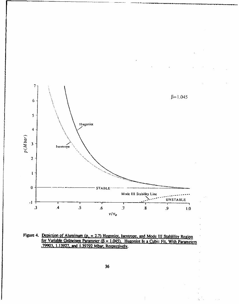
4. Depiction of Aluminum (p0 = 2.7) ltugoniot, Isentrope, and Mode III StabilityRegion for Variable Girneiscn Parameter (3 = 1.045). Hugoniot Is a CubicFit, With Parameters .79903, 1.13927, and 1.39792 Mbar, Respectively .... 36
LIST OF TABLES
Table Page
I. Comparing Internal Energies Resulting From Consiant Compressibility "Isentropic"and "Tensile Shock" Expansions ............................... 21
2. Values of Compression, Relative Volume, and Normalized Values of Sonic Velocity,Pressure, Tangent Bulk Modulus, and Secani Bulk Modulus, Respectively, for theProposed Tension Limiting Model, With g = 20 .................... 23
V

INTENTIONALLY LEFT Br ANK.
I v
iV

I. INrRODUCTION
With the widespread use of numerical (hydro-) codes to describe the behavior of bodies impacting
at high velocity, it is vital that code developers and users be familiar with the various numerical
models in the codes. All too often, cffort is concentrated on the "numerics" of a code, such as
integration and discretization techniques, artificial viscosity formulations, mass lumping and pressure
averagi ng techniques, and mass advection schemes. with the same rigor being absent when considering
the "physics" of the code.
Because code development involves significant effort, it is common for codes to evolve or be
passed down directly, rather than be written from the ground up. With this sort of evolution, it ispossible to avoid "reinventing the wheel." Unfortunately, this mentality, if taken to the extreme,
precludes the ability to redesign the "wheel" and can result in an incompatible combination of "wheel"
and code "e-chicle." Common problems associated with material model evolution are enumerated
below:
(1) Many materia" models are based on assumptions and limitations which are often not passed onwith the model. Thus, material models which are valid only for a particular class of problems
Ce.g. small compression, ductile behavior, etc.) can be erroneously applied to more general
classes of problems.
(2) Goodness of a material model is often judged on its ability to solve a particular set ofproblems, rather than on adherance to fundamental principles. Such heuristic approaches
(e.g., use of non-associated flow rules) can be exercised with caution but often become
institutionalized and taken as fact by an unknowing community.
(3) Many new material models are derived by applying ad hoc modifications to older models,
rather than rederiving the models from basic principles. When this is done carelessly,
conflicting assumptions or limitations can render such models invalid.
(4) Material libraries tend to take on a life of their own and are passed down from generation to
generation without the accompanying experimental data used to generate those libraries.

When this happens, material data are often used under conditions (e.g., strain rates, pressures,
etc.) where those data arc not valid.
One aspect of material modeling which is extremely important to impact codes, and to which all of
the abovementioned problems are relevant, is the equation of state (EOS). In this report, equations of
state for use in impact codes are discussed in general terms, with the Mie-Grdlneisen equation of state
used for specific illustrative purposes since it is the workhorse EOS of the current generation of
hydrodynamic wave codes. Basic derivations, assumptions, and limitations of applicability are all
discussed, with the prime focus being on equation-of-state stability.
2. THERMODYNAMIC STATES AND THE EQUATION OF STATE
To completely describe the volumetric behavior of a material, the values of the thermodynamic
state variables (i.e., the thermodynamic coordinates) are needed for every state of the material.
Thermodynamic state variables are properties which are only dependent on the state of a material and
not on the path taken to arrive at that state. Examples of typical thermodynamic state variables
include pressure and temperature, as well as specific volume, internal energy, enthalpy, entropy, etc.
To describe the state of a simple substance, excluding such phenomena as phase change,
dissociation, or electromagnetic work, a knowledge of the material's pressure, as a function of density
and temperature, is sufficient to completely describe the state of a material. In general, these
thermodynamic state data are related in one of three forms.
Tabulated experimental data is one popular form of representing thermodynamic state data. Steam
tables are probably the most widely used form of tabulated thermodynamic data. Data are tabulated
over a large range of states, and interpolation becomes necessary to obtain data between the tabulated
state points.
Of a similar nature to tabulated thermodynamic data Is graphical thermodynamic data. The
Mollier diagram, which graphically represents the states of water In Its various phases, Is the classic
example of graphically rcprescnted thermodynamic data. To the experienced user, graphical state
tables provide a fast, accurate means of evaluating the change In state variables, When something Is
2

known about the thermodynamic process in question. Like tabulated data, extensive experimental
testing is necessary to generate the data found in graphical thermodynamic state tables.
The third, and possibly most common, way to represent thermodynamic state data is in analytical
form, and is referred to as an equation of state. Traditionally, the EOS expresses pressure in terms of
density and temperature. Describing material by way of an EOS has many advantages. The form is
compact, much more so than exhaustive tabulated data. An EOS may be mathematically codified, thus
making it the most attractive on the basis of programming considerations. Additionally, the
interrelationship of state variables may be mathematically derived, from the EOS, thus providing a
more fundamental understanding of the thermodynamic phenomena at work.
On the other hand, equations of state can suffer from severe deficiencies, which can make their use
prone to error. Invariably, equations of state are formulated, with a host of inherent assumptions about
the nature of the material behavior. Common examples of such assumptions include constant specific
heats, ideal gas, etc. While these assumptions may be valid over a smaU domain of possible states,
they are often poor at describing the material under extreme thermodynamic conditiotts like high/low
pressure, phase change, and the like. This limitation, in and of itself, is not bad. However, those who
use these equations are not always cognizant of the conditions under which a given EOS is valid.
Thus, equations of state may be used in a thermodynamic domain where the EOS parameters are no
longer valid. Also, there can be a problem with EOS forms which, though capturing the essence of
the material behavior, suffer from "higher order" inconsistencies that only manifest themselves
obliquely.
When it comes to hydrocode modeling of material deformation, where the EOS is just a means to
a computational end, sophistocated equations of state, though available in the literature, are rarely used
because of simplicity (i.e., efficiency) considerations. This focus on computational simplicity merely
serves to enhance the likelihood of EOS failure in hydrocode computations.
All equations of state need data with which to drive themselves. In the case of the Mie-Grlneisen
EOS, as used in today's hydrocodes, thermodynamic state variables an: expressed relative to those
states found along an experimentally determined pressure-volume curve which, for the case of impact
data. is usually chosen as the Hugoniot curve. Thus, before the Mie-OrUneisen EOS can be discussca
3

-__
in detail, the reader must acquire an appreciation of the Ilugoniot and the thermodynamic process of
shock transition.
3. SHOCK TRANSITION: A THERMODYNAMIC PROCESS
A shock is a volumetric disturbance vhich travels faster, in a medium, than the bulk speed of
sound (i.e., sonic velocity) characteristic to the state of that medium. A shock is characterized by a
shock front, which itself is very thin (thickness on the order of micrometers), and is analytically
idealized as a discontinuity in physical properties such as density, pressure, and energy. The thinness
of the shock coupled with the high velocity of the shock front ensure the adiabatic nature of shock
transition. Large amplitude disturbances are not necessarily shocks if the thickness of the disturbance
is relatively large. Correspondingly, the amplitude of a shock need not be necessarily large as long as
the disturbance is traveling faster than the sonic velocity.
Shock transition may be thought of as an adiabatic irreversible thermodynamic process which
permits the state of a material to be altered in a fashion similar to isentropic, isothermal, isochoric,
isenthalpic, and isobaric processes. Whereas all of these other thermodynamic processes are
characterized by the constancy of a particular state variable, the process of shock transition is
characterized only by the existence of a shock wave. No thermodynamic state variables remain
constant during shock transition. Nonetheless, the shock transition process can be as well
characterized as any of the other thermodynamic processes, as will be shown from the following
derivation of the basic shock relations.
4. BASIC SHOCK EQUATIONS
Consider a shock disturbance traveling at velocity U, into a stationary medium, with density,
pressure, and specific internal energy of p,, p,. and E0 , respectively. Behind the shock, the material
has acquired a particle velocity, given by up, traveling in the same direction as the shock disturbance.
The density, pressure, and specific internal energy are p, p, and E, respectively. This situation is
depicted in the Laboratory Frame diagram of Figure 1. If an observer could be situated right on the
shock wave, so that the shock were to appear stationary, the situation would appear like that depicted
4

0C) II
V 0E
N 1~
o-
-, C)
I CQ
IICu
D
~IIii~
C
2 ~
C
.2 /U
5

in the Stationary Shock Frame diagram. The continuity, momentum, and energy relations are derived
below by considering an infinitesimally thin contol volume, which fluxes mass dM, over a time
increment dt, which straddics the shock front, in the stationary shock frame. The control volume
projects unit area A onto the shock front.
CONTINUITY:
Mass In poUA dt
Mass Out: p (U, - A di
p~U,Up u,
Or, in terms of compression t:
ooo! up; where I - 1
MOMENTUM:
Decelerative Impulse: (p -P) A dt
Momentum Decrease: dM [U, - (U,-up)] = (p. U, A d) [1U, - (U,-yu]
p-p.=poU,u.; for p°-O, p=p.Uup
EN"ERGY:
Energy In:
Internal Energy In E, dM = E. (pU. A dt)
Kinetic Energy In : 112 dM U, = 1/2 (p. U,, A do U
Net Work on Control Volume: IF dx = (p, A) (U, di) - (p A) [(U,.u) di)
Energy Out:Internal Energy Out E r dM I. (pE U, A dt)
6

Kinetic Energy Out • 112 dM u= 112 (p. U, A dt) (U5-u)2
Internal Energy Accumulated: 0
F - E, = 1/2 (p + po)(l/po - i/p); for p. 0, E -E. = 112 p(l/p - lip)
Or. in terms of compression I:
E-E, = (P;P) t' forp.-0, E-E o - P 92p. (I + gt) 2p. (I + Vt)
5. THE IlUGONIOT
The momentum relation derived above expresscs pressure in terms of shock and particle velocities,
Us and up, respectively. If the nature of the shock or particle velocity relationships are explicitly
known, then the pressure can be expressed in terms of specific volume v, density p, or alternately,
compression p. This pressure-volume relationship for the shock compression process is called the
Rankine-Ilugoniot equation-or more simply, the Hugoniot-and is the locus of states which can be
achieved through the shock transition of a material from a given (p,, v,) state.
It is vital to note that the Hugoniot does not represent the actual path of states through which a
material progresses, when transitioning from the (p., vo) state to (p, v), but rather the locus of final
(p, v) states which can be achieved through shock transition. Also, since we know shock transition to
be a compressive proccess only, a particular Hugoniot curve has one endpoint: the pre-shocked
(p0 , v,) state. From this endpoint, the Hugoniot proceeds in the direction of increasing pressure and
decreasing volume.
Examining the shock energy relationship for the case of an infinitesimal shock, it is seen that
dE = -p0 dv, which exactly equals the reversible work that is done on the material during the
infinitesimal compression. This condition makes the process reversible adiabatic, thus isentropic. The
implicaion is that at its cndpoint, the Ilugoniot is tangent to the iscntropc through that point. Except
7

at its endpoint however, the Hugoniot slope (with respect to dcnsity) is necessarily steeper than theisentrope through a given point.
Unlike other thermodynamic processes, for example isentropic compression, where knowledge of a~single state on an isentropic (p, v) curve is sufficient to completely describe that isenitropic curve,
knowledge of a state point on a Hugoniot curve is not sufficient to define the Hugoniot curve. That is
to say, there ar many (po, v,) states which can possibly shock transition to state (p, v). This isidetical to saying that there are many 1-lugoniots through any state point, as we shall prove in the nextSection.
6. SOME PROPERTIES OF THE HUGONIOT
To prove the assertion that there is no unique Hugoniot through the state point (p, v), let usassume the contrary and show an inconsistency. Consider the Hugoniot referenced to state (p,, v,)
(we will hereafter call this the (p0 , vo) Hugoniot) which goes through state point (p, v). , Consider also
another Hugoniot, referenced to state (P, v,), which also goes through state (p, v). If one assumes
that there is a unique Hugoniot which goes through the state (p, v), then one is forced to conclude that
both states (po, v,) and (P1, v,) lie along this unique Hugoniot. If (p, v,) is in fact on the (po, v,)
Hugoniot, then shock transition can theoretically occur from the state (p, v0) to (pl, v,).
To show the inconsistency which arises from this assumption, consider the changes in specific
internal energies which arise when shock transitioning from states (p, v,) to (p. v), from (p, , v,) to
(p. v) and also from (p, v ) to (P. v,).
E - E, 1/2 (p0 + p) (v, - v),
E - E, =112 (p1 + p) (v,. v)
El- E 1/2 (p. + p1 ) (y. - I
Subtracting the second two equations from the first should produce an identity, but it can be readily
seen that not all of the terms cancel:
8

0= 1/2 [p, (v - v) + p (v0 - vI) - p, (v .
This can be reduced to:
(P] " P,) / (vo - vI) = (P - PI) I(v - v) .
Not only is this expression not an identity, but it will only reduce to a true statement if the Hugoniot
coincides with a Rayleigh line, which is line of constant slope in the (p, v) plane. Additionally,
thermodynamics tells us that there exists a local maxima of entropy along a Rayleigh line, where it is
tangent to an isentrope. Thus, the Hugoniot cannot possibly lie along a Rayleigh line, for to do so
would imply decreasing entropy with increasing shock strength as the shocked state moved beyond the
local entropy maxima on the Rayleigh line.
Thus. the inconsistency has been shown, and one can conclude that the assumption that both
(p0, v.) and (P,, v,) lie on the same unique Hugoniot must be false, even though the Hugoniots
originating at both these points intersect at the point (p, v).
A corollary to this point is that, if one were to proceed from state (p, v.) towards a specific
volume of v, by way of two shocks, the final pressure will not be the same as when specific
volume v is achieved through a single shock, since the new Hugoniot originating at the intermediate
shocked state will differ from original (p0, v.) Hugoniot. In the limit, if the specific volume v is
reached through an infinit, number of infinitesimal shocks, it should not be surprising that the path of
compression will lie along the isentrope through the original (p0, v.) point, since an infinitesimal sho,.k
was shown previously to be isentropic.
In practice, only a single Hugoniot is experimentally determined to characterize the behavior of a
material-that Hugoniot which has as its (p0 , v) state ambient conditions of pressure and specific
volume. Thus, references to "the" Hugoniot for a material refer to a particular "reference" Hugoniot
which has as its origin the ambient (p,, v,) state.
7. EXAMINATION OF SEVERAL HUGONIOT FORMS
7.1 Constant Sound Speed. Constant sound speed implies that all disturbances travel at the same
velocity, or
9

U = Co.
Determining the particle velocity from continuity gives
up = C0 (I - pjp).
It is clear that the particle velocity can never exceed the shock velocity and simultaneously satisfy
continuity, so the implication is that the maximum possible particle velocity is also the shock velocity
C,, and this only occurs as the shocked density becomes infinite. It should be clear from momentum
considerations, therefore, that the maximum pressure achievable in a constant sound speed medium is
p0 C02. Indeed, the relation is given by
(1 +p;)
7.2 The Ideal Gas Form. Much of the work done in thermodynamics is done on the assumption
that the working medium may be approximated as an ideal gas. Unfortunately, at large compressions,
materials do not generally behave in an ideal fashion. Nonetheless, we examine the Hugoniot form for
the sake of academic interest.
An ideal gas is one which obeys the EOS p/p = RT, where R is the gas constant, and T is the gas
temperature. Additionally, an ideal gas is assumed to have constant specific heats cp and c. Under
these conditons of idealness, E = c, T, and the EOS may be expressed as p/p = (R/c,) E. But
R = c - c, by definition, and the ratio c1 /c, is often expressed as y, so that
p = p (y - 1) E.
Cons dcr the shock energy equation, and eliminate energy terms from it by substituting the gamma law
from above. In that case,
PA P.Ph P = (p, +ph) (ip. - I/P)p(Y- I) po(Y -1)
10

This may be solved for the Hugonio, pressure ph~, and expressed in compression form, by substituting
(I + li) for pip0, to give
-Y ( 1 ) -(Y - ) 0y-0
Exprcssed in a (p p) form, 1t becomes
ph -P, 2y l2 - (y - 1) lt
ris Ilugoniot form is seen to approach infinite pressure when
p = /y- 1)
This limit, expressed in termns of dcnsity, is
Y -i
7.3 The Linear U.. u_ Formn. It has been empirically observed for many materials, over a
significant range of pressures, that the relationship between the shock and particle velocity can often
be fit by a straight line, as in
us = C. + S uP.
Thus,
ph -P. P, (C. +SISU u

and from continuity, panicle velocity may be determined as
U ,wherer = 1-p 0 p.I 1-rnS
Particle velocity may be eliminated from these equations to give
: 2-'
P. C.o 1ph -P.(1 S) 2
Expressing this in compression form gives:
P" C L(I + V&)i ~ ( S -1) 11) 2
It can be seen, for S > 1, that this linear U, - up llugoniot equation approaches infinite pressure at
finite compression (t I/[S - 1]), not unlike the ideal gas EOS. Otherwise, for S < 1, the Hlugoniot
pressure converges to p Co2/(S " 1)2 for large I. Also, the special case of S = 0 reduces to the
previously derived situation of constant sound speed. This finite limiting pressure for S < I arises
because the U. function intersects the up function at U, = Cj(1 - S). Since U, must always exceed up,
these limiting values of U, and u, cause the limiting value in pressure too. Though this U, =u
condition is unrealistic, apparently several materials exhibit S < I at lower compressions (Kohn 1969).
Such data can be misleading, and can cause problems if S < I is retained out to larger compressions in
numerical simulations.
7.4 The Polynomial Hugoniot. Often, a form is not assumed on the U, - u relation, or the
compressibility at all, but rather, an empirical fit is made directly to the Hugoniot, as in
p,,-, PO K, V' ,
where Ki are the empirical constants, and n is the order of the polynomial fit. A popular value
for n is three, giving a cubic fit. Note the functionally different forms between this lugoniot form
and the linear U. - up form, for instance. To work the problem in reverse, and obtain the shock
velocity for a cubic Hfugoniot fit, for example, one can manipulate continuity and momentum
equations to get:
12

[K1 (K1 + K) ~ ( 2 +K 3 ) p2 + K3 113] Ip
Note that U ' at g = 0. which is C. 2 , cquals K,/P,.
8. THE IMPORTANCE OF DISTURBANCE VELOCITY ON NUMERICAL STABILITY
Tht, primary emphasis in describing the shock !oading behavior of materials has been on the
ttugoniot fit itself, the Ph VS. gX relation. However, the importance of the disturbance speeds U,
and C i.e.. the shock velocity and local sound speed) cannot be underestimated. In impact
computations, where the wave motions are the important part of the problem solution, knowledge of
disturbance velocities becomes necessary for accuracy, and in explicit schemes, for stability, of the
calculation.
In explicit integration schemes, which arc by far the most prevalent in use for impact calculations,stability requirements place limitations on the integration timestep. In particular, the explicit
integration timestep must be limited so that a disturbance can traverse no more than a single
computational zone per integration cycle. To enforce this requirement, one needs knowledge of both
the particular zone size in question and the disturbance velocity in that computational zone. The
former is simply a function of zone geometry, while the latter is the shock velocity U, when the
material is compressing, and the sound speed C, when the material is expanding. Thus, an accurate
knowledge of disturbance velocities U and C, under various states of loading, is vital to the numerical
stability of explicit integration schemes.
In addition to the effect of the disturbance velocities on the stability of the explicit numerical
integration scheme, these velocities are intimately related to the stability of the EOS calculation itself,even in the absence of a numerical code application. There are thermodynamic considerations which
must be satisfied by any valid EOS.
Three particular modes of EOS instability will be addressed in the following sections. Stated inEnglish. these stability criteria sound almost trivial, since they immediately result from fundamental
thermodynamic statements, which have been known and professed for years. Nonetheless, these
13

criteria, which can be expressed mathematically, and are tested in the framework of the Mie-Grnneisen
EOS, show a necessary interrelation amongst various EOS parameters, which is not commonly
appreciated. As such, indiscriminate choice of parameters to drive the EOS will often cause at least
one of these criteria to be violated. Use of such data in a numerical scheme can result in bizzarre
manifestations of numerical instability.
The three stability criteria are given below and apply to materials where phase changes and/or
porosity are not considered (i.e., simple substances). For the first two criteria, consider a state (p, v),
which lies on the Hugoniot originating from the state (p0, v0).
(1) at the state (p, v), the slope of the Hugoniot with respect to density must exceed the slope of
the Rayleigh line connecting states (p., v.) and (p, v);
(II) at the state (p, v), the slope of the isentrope must lie between the slope of the Hugoniot, and
the slope of the Rayleigh line connecting states (p0 , v.) and (p, v);
(IIl) the slope of an isentrope with respect to density is always greater than zero.
From the second law of thermodynamics, it is known that entropy is monotonically increasing along a
Hugoniot. By definition, entropy is constant along an isentrope. Finally, a Rayleigh line is known to
have one point of maximum entropy. It can be shown (Zuker 1977) that this point of maximum
entropy lies between the states (p., v,) and (p, v). Thus, at the state (p, v) and traveling in the
direction of increasing density, entropy must be decreasing. Criteria I and II express this relational
placement of the Rayleigh line, the isentrope and the Hugoniot. Criterion III simply implies the
obvious, that the speed of sound in a material is a positive quantity.
9. MODE I INSTABILITY OF SEVERAL HUGONIOT FORMS
It was mentioned that a Hugoniot has the slope (with respect to density p or compression g.) of the
isentrope only at tie end point of the Hugoniot. At other points along the Hugoniot, the Hugoniot will
always be steeper than the corresponding isentrope. Let us examine the two most popular Hugoniot
forms (linear U, - UP fit and cubic fit) to check their adherence to these rules. The slope of the
14
Hugoniot at any point on the Hugoniot is simply dpdp. Total derivatives are used since, along the
Hugoniot, pressure is only a function of a single variable (p, i, or v, at the discretion of the user). To
determine thc slope of the iscntrope at that point, one can make use of the definition that dp/lp ,
equals the square of the sonic velocity.
For the case of the linear U, - up lit, recall that
2ph - PO- (1 -(S-1)g) 2
Taking the derivative with respect to i, one may obtain
dp poC, I - (S - 1) pldp [I (S - 1)
The chain rule dictates that dph/dp = dp,/dt dwi/dp. where dlpdp is simply I/p0, so that
dph C2 [1 +(S+ 1)]dp [I - (S- 1) 111,
Without knowing additional information about the EOS, the slope of the post shock isentrope
apIap I = C2, and, thus. the sonic velocity C, cannot be explicitly determined after a shock.
However, the particle vclocity relative to the stationary shock front after a shock, equal to (U, - u), is
known to be subsonic. It may also be shown that o~p/,p along the Rayleigh line connecting the pre-
and post-shocked states exactly equals (U, - ud . If the Hugoniot slope is larger than the slope of the
actual isentrope, then clearly its slope must be larger than that of the Rayleigh line, which represents
the lower bound on the slope of the isentrope.
From continuity, the quantity (U, - u) may be expressed either as U,/(l + gt) or u.. Thus, the
slope of the isentrope .)p/ap I, = C2 mu.;t be greater thn U, 2/(l + I)2, which is the slope of the
Rayleigh line. Now, consider the Rayleigh line slope at some point on the Hugoniot. For the linear
U, - up assumption, U, : C0 + S up. However, it is desired to obtain U, in terms of compression I.
15

Elimination of up from the continuity equation gives,
Up (U, -oQ/ Su- up U= -(U,-C.)/S
Upon solution for U,
U. C'(1 +P[ (-(s-1) P]
Thus, )p/ap IR = U2/(l + g)2 and is given as
ap -_ c.p . 11- (S-_1) p]2
For the Hugoniot slope to exceed the corresponding Rayleigh line slope for all g > 0, the ratio of
dph/dp to ap/p R must always exceed unity. Failure to do so implies that there can exist no valid
equation of state to describe the material. We will call Hugoniots whose slope does not exceed that of
the corresponding Rayleigh line, as Mode I unstable. Mathematically, the condition is stated below:
MODE I CRITERION:
dp~/dp > 1, for p > 0, along the Hugoniot.ap/ap I=
For the linear U. - uP form, the stability ratio, which must exceed unity, is given by
dp=tdp [ +(S+I)pJ > 1, for g > O, along the Hugoniot.
aplapl, [ -(S-IJ
Clearly, for any S greater than zero, the stability criterion is not violated. Thus, the linear U. - UP
formulation is always Mode I stable.
16

Considering now the cubic empirical Hugoniot fit, it is of interest to see how this Hugoniot form
fares with the Mode I stability criterion. Mimicking the operations performed on the U, - up forms,
dm/dp is determined as
dph-a;- = K + 2K2I+ 3K3?&2]/ p
The slope of the Rayleigh line. p/ap I R equals U, 2/(1 + .) 2 , and is given by
ap I K, + (K, + K2 ) I + (K2 + K3 ) P 2 + K3 I 3
pIt p, (1 + p)2
Finally. the Mode I stability criterion, which insures that the slope of the Hugoniot exceeds that of the
Rayleigh line connecting the pre- and post-shocked states, is given as
dph/dp _ (K, + 2K2 p + 3K3 i 2) (1 + I) 2 >1
aplapI, K, + (K 1 + K2) P + (K2 + K,) P2 + K3 p3
for g > 0, along the Hugoniot. Because of the dependence of this term on three independent
parameters, a simple answer cannot be given. However, the data collected and fit by Kohn (1969) into
KI, K2, K3 form can still be checked for slope violations. It was found that 21 of 77, or 27%, of the
materials violated the criterion in part of the compression range where the empirical fit was supposedly
valid. Perhaps this behavior can be attributed to the forcing of a cubic Hugoniot function onto a
highly non-linear material response, possibly due to phase changes. In such cases, Mode I instability
implies that a cubic Hugoniot fit is inadequate. The ramifications of Mode I instability on
computational stability are no: as clear as the other modes to be discussed, where instability is more
likely to guarantee computational catastrophe.
10. IN'TRODUCTION TO THE MIE-GRONEISEN EQUATION OF STATE
Traditionally, an EOS is an equation which describes the pressure of a material as a function of
density and temperature. It is needed to solve the continuity, momentum, and energy equations which
govern the thermodynamic transition of a material. In the case of impact though, thermodynamic
17

states change so rapidly that there is little time for heat transfer. Under these conditions of adiabatic
transition, the energy cquation need not explicitly contain temperature, and the governing equations
may be solved if either the entropy or the internal energy is known as a function of pressure and
density (Zeldovich and Razier 1966). The Mie-Griineisen EOS is of this variety, in that internal
energy, and not temperature, is related to pressure and density. The penalty for not having the
traditional p (p, T) formi lation is that temperature is not a computable state variable.
For impact calculations, accurate description of shock transition states is very important.
Additionally, high pressure material data are usually obtained from shock transition experiments and is
given in the form of a Hugoniot curve. The flugoniot provides the means to ascertain the pressure
and internal energy as a function of compression for those thermodynamic states which can be
achieved through shock compression of a material.
Thus, realizing tha! an EOS is only an approximation to the actual behavior of a material, it seems
desirable to have an EOS which is very accurate along the path where data are available (i.e., along
the experimentally derived Hugoniot). State points other than those found directly on the Hugoniot are
obtained from an EOS which references material back to the state along this reference Hugoniot. The
Mic-Grilneisen EOS provides the framework through which state points can be tied back to an
arbitrary reference function, as described below.
Consider the textbook form of the Mic-Grilncisen EOS (McQuarrie 1976), expressed in terms of
density
P - p 2 dU + rp(E-U),dp
where U is the specific interatomic potential energy (a function of density only), and E is the specific
internal energy comprised of both interatomic potential (i.e., compressive) energy and atomic
vibrational (i.e., thermal) energy. Note that the term p2 dU/dp represents the "cold pressure." which is
that pressure arising from compression at absolute zero temperature, in the absence of specific
vibrational intcmal energy (E-U). The term r is the Grlnciscn coefficient, which Is a function of
density only, derived by assuming a particular form on the vibrational frequencies or the crystal lattice.
If the cold pressure curve is known (or assumed), ,nd if the thermodynamic states a known
along another reference curve (e.g.. Ihe IHugonlot), then the Grolnciscn coefficient may be Inkrred
18

directly, :as a function of density. On the other hand, if the thermodynamic states arc known only
along a "non-cold" reference curve, but if a functional relationship is assumed foi the Grtinciscn
coefficient, then the interatomic potential function may be implicitly removed, by referencing the
thermodynamic state at any point (p. p, E) back to the state along the referencc curve, at the same
density (Wf' p. E,cf). This is done by taking the difference of the Mie-Griineisen EOS, given above,
at the two state points in question. It is this approach which is almost universally adopted by
hydrocodes, to give
(p - p,,) = r p (E - Er,).
It should be noted that the interatomic potential, U, and thus the cold pressure curve, may be
recovered, by solving the following non-linear ordinary differential equation:
dU ru = (p)dp p p2
where 0(p) is a function of density only. obtained from the "non-cold" reference curve and the
assumed Grincisen function:
(p) =p,,- rpE.
For the present purposes, the reference function is chosen as the Hugoniot, so that the Mic-Gruincisen
EOS becomes
(p - P) = F p (E -E).
The quantities ph and Eh are the pressure and specific internal energy of the reference Hugoniot state
point at the same density as the state (p, p, E) in question. Often, the shock energy equation is
substituted directly into the Mic-Griincisen EOS to give
p -- p,(o -rg12) + p,r (1 + p) [E - E,] - porp12.
The ambient conditions p0. E.. are generally pegged at zero, so that the Mie-Grineisen EOS, with
Hugoniot reference, is expressed as
P p (- rpl2) + p*r (I + p) E.
19

Note, in an analogous fashion to thc Mic-GrUnciscn EOS, that ideal gas behavior may be modeled
if Iap) , given by r for solids, is held constant for gases, equal to (y - 1), and if the Hugoniotp aEr[
form is that for an ideal gas; namely,
At -P, 2y IP, 2-(y-1)IL
The Mie-Grunesien EOS, with Hugoniot reference, is only valid where the Hugoniot reference is
valid. If the reference Hugoniot is obtained by shocking material from ambient conditions, then
clcarly the Hugoniot is only valid in some region g > 0. Hydrocode implemcntors often fail to deal
with this fact accurately. It is well known that the Hugoniot curve is a very close approximation to
the isentrope at small values of compression, and so the pressure reference function usually employed
by hydrocodes in tension is the isentrope, which is generally approximated by a curve which matches
value and slope of the Hugoniot at g± = 0. There is nothing wrong with this assumption, but
innaccuracies are introduced when the shock energy equation is still employed directly to compute the
energy reference function, as in EPIC (Johnson, Colby, and Vavrick 1978), which is tantamount to
assuming the existence of a tensile shock.
Clearly, the energy reference function to drive the Mie-Griincisen EOS in tension should not be
the shock energy equation
EL -E, - P~v(whL po. ),2 p°(1 + p)
but rather some physically plausible function-for instance, the isentropic expansion integral of work:
I
oV p° E. f p,)
One possible approximation for the iscntropic release function for It < 0 is to assume constant
compressibility. In this case, where p, = E, = 0 is assumed for simplicity.
20

pr=K, L, and
Ee --foP __o__ _) - (K/p,) [In (I i) -p/(1 - p)]
Comparing the internal energy from this reference function to that computed from the invalid
application of the shock energy equation in the tensile region, given by
E 2. - 2 I
one may obser-e that thc difference in computcd internal energies is significant, as shown in Table 1.
TABLE I. Comparing Internal Energies Resulting From ConstantCompressibility "Isentropic" and "Tensile Shock" Expansions
Sp. E/Ko p. Eh/KoVV (isentropic) (tensile shock) % Error
0.0 1.00 0. 0. 0.
-.2 1.25 0.027 0.025 -7.4-.4 1.67 (.156 0.133 -14.7-.6 2.50 0.584 0.450 -23.1-.S 5.00 2.39 1.60 -33.1
Other reasonablc choices of isentropic release pressure reference functions may also be used in the
rcgion .t < 0. For example, let the reference sound speed for a material in tension (g < 0) be
described with the following function:
C v C,(1 * ,.
For this particular sound speed reference function, the tangent bulk modulus may be computed as
K = K. (I + p)14")
21

This function has many nice properties. Two such advantages are that it reduces to constant
compressibility for g = -1/2, and to constant sound speed for g = 0. Additionally, the sonic velocity is
at the proper value at .= 0 and, for g greater than zero, the sonic velocity drops off to zero when the
material is infinitely expanded (at g = -1). Increasing the exponent g causes the sonic velocity to drop
off more rapidly in tension and will limit the maximum value of tension achievable during an
isentropic expansion, which is a material feature observed experimentally and often modeled
computationally by way of a pin parameter. The reference pressure function is acquired by
integrating the tangent bulk modulus and is given below for g not equal to (-1/2):
,, K = _ [(1 1].f (1 + p) 2 (2g + 2)
The reference energy function (for g not equal to -1/2) is acquired by integrating the reference pressure
function:
.E [(1 f -,). K_ 11 - it (2g + 2)0 P.0l - p.) (2g - 2) (2g + 1) (1 * pt)
For the special case of constant sound speed adiabatic expansion from . = 0, the exponent g equals 0,
and one gets:
p, - K°(i + 2 )/2 , and
W - 2p, (lI )
On the other hand, the reference pressure may be limited to a tensile pressure of Pmin, which occurs at
infinite expansion, by defining the exponent g to be
9 K°2 I&1 .
22
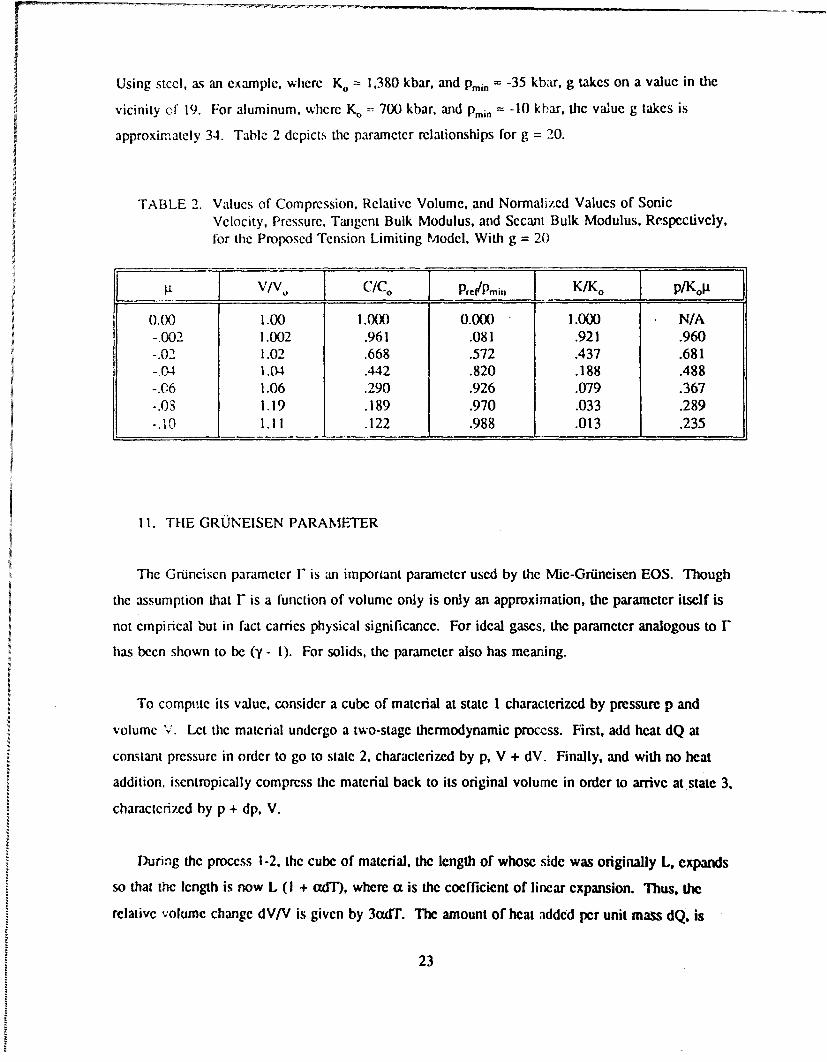
Using steel, as an example, where K. = 1.380 kbar, and Pmin = -35 kbar, g takes on a value in the
vicinity of 19. For aluminum, where K, = 700 kbar, and Pmin = -10 kbar, the value g takes is
approximately 34. Table 2 depicts the paramcter relationships for g = 20.
TABLE 2. Values of Compression, Relative Volume, and Normalized Values of SonicVelocity, Pressure, Tangent Bulk Modulus, and Secant Bulk Modulus, Respectively,for the Proposed Tension Limiting Model, With g = 20
T V/V0 C/Co PrcPmn K/Ko P/K0 p
0.00 1.00 1.000 0.000 1.000 N/A-.002 1.002 .961 .081 .921 .960-.02 1.02 .668 .572 .437 .681-.04 1.04 .442 .820 .188 .488-.06 1.06 .290 .926 .079 .367-.08 1.19 .189 .970 .033 .289-.10 1.11 .122 .988 .013 .235
11. THE GRONEISEN PARAMETER
The Gruneiscn parameter F is an important parameter used by the Mie-Grilneisen EOS. Though
the assumption that F is a function of volume only is only an approximation, the parameter itself is
not empirical but in fact carries physical significance. For ideal gases, the parameter analogous to F
has been shown to be (y - 1). For solids, the parameter also has meaning.
To compuite its value, consider a cube of material at state I characterized by pressure p and
volume V. Let the material undergo a two-stage thermodynamic process. First, add heat dQ at
constant pressure in order to go to state 2, characterized by p, V + dV. Finally, and with no heat
addition, isentropically compress the material back to its original volume in order to arrivc at state 3,
characterized by p + dp, V.
During the process 1-2, the cube of material, the length of whose side was originally L, expands
so that the length is now L ( + adT), where a is the coefficient of linear expansion. Thus, the
relative volume change dV/V is given by 3WET. The amount of heat added per unit mass dQ. is
23

Cr dT. For solids, which are nearly incompressible in comparison to gases, the specific heats at
constant pressure and volume, cp, and c, are nearly identical. Thus, the heat added can be
approximated by c, dT. The temperature change dT may be eliminated by relating dT back to volume
change dV so that
c dVdQ=--
3acV
The work done by the material per unit mass is negative since the volume change is the opposite sense
of the pressure loads and is given by dW = -p dV/(pV). From the first law of thermodynamics, the
internal energy change dE, given by dQ - dW. can be expressed as
dE cdV pdV3aV pV
The process from state 2 to 3 has no heat addition, so dQ = 0. The work done by the system is
dW = (p + dp/2) dV/(pV) which, to the first order, is p dV/(pV). The rise in internal energy is
therefore the negative of the work
p (-dV)| pV
Thus, the difference betwecn the pressures going from state I to 3 is dp, and the rise in internal
energy is
c,,dVdE13 = 3d
The volume of states I and 3 are identical, so that the Gninciscn parameter r will remain constant for
the direct transition from state I to 3. when using the Mie-Grfnciscn EOS, which relates states I and 3
as follows:
---r p --
- (dV) 3aV
24

But path 23 is isentropic, so that dp/(-dV) is )p/aV I, = (-p/V) op/lap I,. But o)p/)p 1, is simply the
square of the sound speed C, or alternately, the ratio of the bulk modulus and the density K/p.
Substuting, and solving for r gives
r 3 C2 3a KCV P CV
From the Mic-Grdnciscn EOS, it is clear that the Griinciscn parameter F relates changes in internalenergy to changes in pressure at constant volume. As can be seen from the dimensional analysis of
the second expression for F which follows, the numerator expresses the pressure rise per increment of
temperature, while the denominator expresses the (volume-based) energy rise per increment of
temperature. These terms combine in a way to produce a non-dimensional expression which
represents the Gnineiscn parameter.
dV V dpr-3aK deg dVIV dpldeg dp _
pc dE p dEldeg pdE
Note: As in other places in this document, dE represents energy change per unit mass.
12. MODE II INSTABILITY OF THE MIE-GRONEISEN EQUATION OF STATE
Though there is nothing inherently wrong with the Mic-Griineisen EOS, there are often situations
where inappropriate choice of data forces a thermodynamic violation. As pointed out in the previous
section dealing with Mode I instability, there are certain empirical Hugoniot fits which may violate
fundamental thermodynamic rules. Clearly, plugging such fits into Mie-Grilneiscn makes the
possibility of catastrophic EOS failure significant. Additionally, there are inconsistent combinations of
flugoniot and Grilneiscn functions which cause thermodynamic violations which arm not immediately
apparent.
To study these, consider a material in the state P. p, Eb on the Hugoniot originating at (p,. v).
From this state, consider two possible paths resulting from a small compressive increment, dp: the
25

path along the isentrope and also the path along the Hugoniot. Along the isentropic path, the pressure
change is
ap dp - C dp.
The internal energy change along the same path is the negative of the work, or
dp = p, (dp/p 2 )ap
Along the Hugoniot, the pressure change is simply (dph,/dp) dp, and the energy change, may be
obtaincd by taking the derivative of the shock energy relation Eh - E, = 1/2 (ph + po) (l/P " l/p),
to get
dE
If is ateialist dpyteMeGnic Othna h est pdp 1/2 [(Ph +Po/]P - (1/p0 - l/p) dpAldp] dp
If tl's material is to obey the Mic-Grilncisen EOS, then at the density p + dp.
ph+ dp (Ph +p rdPh do = rP + I, dp -(E, +. dp)j.
Canceling and substituting terms gives
(Ca - dphidp) = r p (ph/p 2 - 1/2 [(Ph + p)1p2 + (i/p. -/p) dp,,Idp]).
Expressing this in terms of compression .t, and solving for r gives
r 2 [, Ii dh)'. -, po0C21p. [ Ii dphfdp - (ph p)I(l -p) p)]
26

The signi ficance of this expression is that, for a given Hugoniot relationship ph as a function of i, the
Gruneiscn coefficient r and the sound speed C arm related. Since the sound speed is known to have
thermodynamic limitations placed upon it. these limitations translate into constraints on the Gnineiscn
parameter F. Use of the Mie-Grincisen EOS in codes, without the appropriate restraints on r, will
usually result in catastrophic failure of the EOS.
To examine these constraints on F. consider the maximum and minimum possible values on C.
Recall that tie post shock particle velocity relative to the shock front, cqual 1o (U, - U), is known to
be subsonic, but approaches sonic conditions for infinitesimal shocks. Thus, as an absolute lower
bound, let C approach (U, - Up. This choice of C gives an upper bound on F. But (U, - u) equals
U,/(l + Ig), so that (U, - ud)2 is given by
(U,- -_,/(1+ (I + (P, -P/[P. V (I +
Substituting this into the expression for F gives, as an upper bound,
r = 2/px
For the lower bound on r, one may assume that the isentrope approaches the HugonioL In this case,
a)p/d. I = dp/dg. Since )p/j. 1, equals p. C2 by definition, the minimum value on I may be
determined as zero. By combining these two criteria, and calling them the Mode II stability criterion,
one gets
MODE I! CRITERION:
o < r < (2/p)
Failure to satisfy this criterion implies that the slope of the post shock iscntopc does not fall
between that of the Raylcigh! line and the Hugoniot.
Recall, from the ideal gas form, that the parameter analogous to F is constant, and equal to
(y - 1). It may at first appear that the ideal gas form violates he Mode H stability criterion for lage I.
However. recall that Infinite pressure was approached when the ideal gas compmssion pt equaled
27

2/(7 - 1). which is 2/F in Mie-Grilneisen terms. Thus, over the physical . domain of tile ideal gas
form, which is g. < 21T, Mode II stability is not violatcd.
In general though, it becomes clear that the terminal value of tie GrUneisen coefficient, let us call
it F,, must be less than or equal to 2/ga1, where Va, is defined as that value of compression which
produces infinite pressure in the Ilugoniot. For the linear Us - uP form, It, occurs when the
denominator (1 - (S - 1) gt) becomes zero, which occurs only if S exceeds unity. In this case,
'a I - (S- 1).
The value of I,, therefore, should be less than or equal to 2(S - 1). For S 1 1, the linear U, - u
form becomes unbounded only as It approaches the infinite. In this case, F must approach zero.
Similarly, for polynomial fit Hugoniots, shock pressure becomes unbounded only when compression
approaches infinity. Thus, the Gruneisen coefficient F should also approach zero, all the while
remaining less than 2/g., as compressions become very large.
It is unfortunate that data for r are generally only available at the ambient gx = 0 condition. As a
result of this, it has been common practice to leave the value of F constant in numerical computations
for lack of better data. In analyzing the data of Kohn (1969). it is observed that none of the data
presented violate the Mode II stability criterion, 0 < r < 2/pg, for the range of i over which the data
are collected. However, should the data be extrapolated to larger values of It, Mode II instabilities
may result, since 100% of the cubic fits, and 74.5% of the linear U, - up fits described by Kohn
(1969) will violate Mode 11 stability at larger p. if r is held constant at its initial value.
13. CORRECTIONS FOR MODE II INSTABILITY
To enhance Mode 1I stability, some code developers have imposed functional forms on the
Gruneisen coefficient. In the case of the EPIC codes, this is not done, and r is held constant at Fo.
As pointed out, Mode ii criterion will be violated for p > 2/1"o. In HULL (Matuska and Osbom
1987), the value of F is a defined as r = 17 pjp, which in terms of compression p, is
28
r = ro/( + P).
This form can still violatc the Modc II criterion if F. > 2 and g > 2/(10 - 2). DYNA (Hallquist
1989). as well as vcrsions of CALE (Tipton 1989), use a first order correction to r o, which is
cquivalcnt to assuming the form on the GrUncisen parameter as
r = (ro+Ap)I(l + p)
where A is a paramctcr which, when fit to EOS data at moderate pressures, is always greater than or
equal to zero and generally lics in the vicinity of 0.5 for most metals (Tipton 1989). If the value of A
is chosen as zero, the DYNA/CALE form for r reduces into that used by HULL. Even though a
positive value for the parameter A might cause the data to fit better at the pressures of interest, it also
has the side effect of lessening stability at larger compression. If A is positive, the limits on
compression which assure Modc II stability are
(2 - To) + 1(2 - r,) 2 + 8 A A > 0.
2A
For materials like aluminum, with r = 2.09 and A = 0.49, the DYNA/CALE Grilnciscn form has a
limiting compression of stability near 2. This value is better than the limiting value of unity, derived
from the constant P = 2 assumption, but is still prone to failure when simulating hypcrvclocity impact.
MESA (Bolstad 1990) uses a form:
r =y + y1/(1 + p)
which is directly convertable into the CALE version, if one takes 10 = (7o + y1) and A = T. Thus,
the arguments made about the CALE form apply to MESA as well.
From the pcrspectivc of assuring Modc If stability, evcn at very large compressions, an altcrnatc
Grilmniscn form, being proposed here is given as follows:
29

r- ro0
1 + j3ji
where 13 is the newly introduced parameter. Unlike the other forms on F. where stability is a
coincidental by-product of the choice of F., Modc ii stability can always be ensured, with the current
form, given appropriate choice of 13. The form reduces to that used by HULL if 13 is forced to unity
and can be made to approach constant F if [3 equals 0. However, constraining 13 to a value greater
than or equal to 1-J2 will ensure, for any Hugoniot form, that Mode II stability is always satisfied for
any finite g.. The constraint on 13 can be relaxed somewhat if the associated Hugoniot form is valid
only in some finite range 0 < p. < p, An example of such a limited domain Hugoniot is the U, -u
form, with S > 1, where 1-x = l/(S - 1). For these cases, the constraint on 13, to ensure Mode II
stability, is
r, - (21 p,,)
2
To see how this proposed form can match the DYNA/CALE form at lower compressions but still
provide stability at higher compressions, Figure 2 is provided. In it, three Griineisen relationships for
aluminum are shown (data for aluminum, I. = 2.09, and S = 1.33 are extracted from Kohn [1969]).
The A = .49 (CALE) curve shows the functional form of F, using the DYNA/CALE functional form.
The value of A = .49 comes directly from the CALE manual (Tipton 1989) and was fitted from
experimental data. At large compressions (in excess of 2), the CALE Grfneisen form violates Mode II
stability. The A = 0 (HULL) curve shows the DYNA/CALE curve for A = 0, which reduces into the
form used by HULL. This form remains stable out to the limit compression, ., = 3, but does not
follow the CALE curve well at lesser compressions, where experimental data were used to fit the A
parameter. Thc 1 = .72 curve, which follows the functional form of the currently proposed model,
follows the CALE curve well at lower compressions, and retains stability out to the limit compression.
Notice that the minimum value of 1, which is guaranteed to retain stability, can be obtained by
substituting FQ = 2.09 and p 1 = 1/(1.33 - 1) = 3 into the equation above. This minimum value is
computed as 0.712, which thus guided the selection of 1 = .72 for the figure.
30

STABLE~ MoNhde 11 UNSTABLE INON-PHYSICAL2- siabiiy LineI
A= ( I UI. )
r,- 2.9 S- 1.33
Figure 2. ComDAdson of OW Waisn Parame Fis fMM CALF, w4d HULL Qdes for Aluminm
With t Qurmidv Pfoaose FItIn -Model, In Llih of Mode 11 Stablity CHer
31

Note that some non-positive values of f0 are permissable. but only if 17 < 2/g', is. true. For a
polynomial llugoniot fit. where it, is ncessarily infinitc, f3 is necessarily positive. One can combine
the 0 constraint directly with the proposed r relation to obtain th re .ation in terms of r,, ji. and li:
2 r.2 + (r. - 211p,) lIi
14. MODE III INSTABILITY USING TIHE MIE-GRUNEISEN EQUATION OF STATE
Mode III instability arises. when the square of the local speed of sound is computed as negative-
a situation which clearly bears no relation to any real phenomenon. In the Mie-Griineisen EOS, it can
arise, because of the fact that the EOS is linearized about some reference curve, which is the
Hugoniot, for impact computations. Since the real world is rarely linear, this idealized linearization
becomes Icss and less accurate the further one gets from the reference curve. When one gets suitably
distant from the reference curve, the thermodynamic data generated from a linearized EOS can be not
only inaccurate but also in violation of basic thermodynamic principles.
When the situation of imaginary sound speed occurs, many codes (EPIC3, for example) reset their
value to zero and merrily continue on their computational way. Unfortunately, the situation can be
much more serious than just computing an inaccurate sonic velocity. An imaginary sonic velocity
implies that an increment of isentropic compression on an element will result in a DECREASE in
pmcssure. Rectting the sonic veloity to zero does nouthing to prcvcnt thc ihemnodynamic state of the
element from going berserk. It is these sorts of situations which most often result in catastrophic
manifestations of instability over the span of one or several computational iterations--ballooning
elements, collapsing elements, and wild energy fluxes are typical.
The local speed of sound is defined as the rate at which an infinitesimal disturbance propagates
through a medium. Expressed by the symbol "C". it is mathematically expressed as:
apap
32

To derive its functional form for the Mie-Grlneisen EOS.
p-ph= rp(E-E))
take the derivative with respect to an increment of density (dp) along the isentrope. This produces the
following result:
ap - dp r p a, - (E -E ) (1'P)ape dp Tp dp )dp
Converting the derivatives into compr.ssion form, this relation may be ultimately simplified, with
energy terms eliminated, to produce the result:
MODE III CRITERION:
C2 r+I I r ) dI. r/D k .
For the special case of p Ph (i.e., along the Hugoniot), this form expresses the relationship derived
for F in Section XI,
2 [pdpId - pp.C']pt [jtdpj,1dpt-(pA,-p.)j(1 + .)1
which was subsequently used to derive the Mode II criterion. Note, however, that Mode III only
requires the sound speed to be positive at all thermodynamic states, whereas Mode 1I required the
slope of the iscntropc (which is directly related to the sound speed) to be not only positive but
greater than the Rayleigh line slope. Thus, the Mode i criterion is more stringent than Mode !II, but
it only applies along a Hugoniot.
Thus. if the Mode Ill criterion is violated at some state, which happens to lie on the Hugoniot
(Ph, I) then the Mode II criterion will have already been violated at that compression it. However,
33

the full Mode IIl criterion gives the opportunity to study stability at all states in the (p. v) or (p, jt)
plane, not just along the Ilugoniot.
Operational simplitications may be possible when applying the Mode III criterion, depending on
the actual choices of the ph and F functions. As an example, if one adopts the functional form for the
Grncisen cocflicient proposcd in Section XII, F = 1,(I + I3.), then the Grtonciscn derivative terms
simplify nicely:
r1 dr r, l+1
Because of the linearized nature of Mie-Grdneisen, there can be states where Mode III stability is
violated However, their occuruace can be greatly rcduced, given an appropriate choice of Ph and rfunctions. As an example, consider Figure 3, which depicts the (p, v) plane cubic fit Hugoniot for
aluminum with coefficients .79903, 1.13927, and 1.39792 Mbar, respectively, and density of 2.7 g/cm 3
as given in Kohn (1969). if F is held constant at its initial value of 2,09, co.responding to 3 = 0 in
the cuterr.tly proposed model, the Mode Ill stability line, which divides the (p, v) plane into stable and
unstable regions. is seen to produce instability in a large part of the (p, v) plane, including
thermodynamic states in which the simulation might reasonably expect to exist. Note that an
isentrope, when it crosses into the unstable region of the (p, v) plane, changes its slope so that
increased compressions actually cause a decrease in pressure. It is this sort of unstable behavior which
will cause a simulation to come screeching to a halt in no time at all.
On the other hand, if 3 is increased to a value which guarantees Mode I1 stability, as discussed in
the previous section, Mode IIl stability is also greatly enhanced. Since a cubic fit Hlugoniot has no
lim;ting vdue of compression, the value of 03 to guarantee Mode I! sLability must equal or exceed
1'/2, which for the case in point (r. = 2.09), is 1.045. With this new value of P, shown in Figure 4,
the unstable region is limited to a very small portion of the (p, v) plane, which represents material
under very large tensions. In fact, the tensions required to produce instability are so large (391 kbar
at v = v., for the case in point), that aluminum's spall pressure would be. exceeded and material failure
would occur before the material was ever able to approach this unstable thermodynamic state.
34

I7
6-UNSTABLE *STABLE
4-
2-
Isentrope ........
.3 .4 .5 .6 .7 .8 .9 1.0
Figre 3I Depiction of Aluminum (p. 2.7) Hugoniot. Isentrope. and Mode M1 Staibi~ty Regtionfor Constant Grifeisen Parameter r = 2,09 (ft = 0). Hug2niot Is a Cobic Fit. WithParameters 73. 1. 13927, and 1.39792 Mbar. Respectively.
35
6 - j31.045
- I-I ugoniot
4
iscntropc
M(Xtc III SaityLine ----
.3 .. 5. 7.8 .9 1.0
Figure 4. Depiction of Aluminum (o 2.7) Huonjot. Iscntrovec. and Mode II1 Stablility Reionlfor Variable Gr~neisen Prmeter B = 1.045). Huoniot Is a Cubic Fit. With Parametcrs,.79903. 1.13927. and 1.39792 Mbar. ResLectively.
36

15. OTHER PROBLEMS WITH MIE-GRONEISEN EOS IMPLEMENTATIONS
Movement of nodes along Lagrangian contact surfaces may produce occasional values of
compression in excess of that anticipated from analytical considerations. Though such artifacts are
purely computational, they can cause the compression to go out of (p, v) domain of known data or,
worse yet, out of the physically plausible (p. v) domain. When this happens, the code may die
instaotly or generate state values so inaccurate as to cause computational "ripples" which disturb the
rest of the otherwise valid computation. This problem can usually be circumvented by forcing a
smaller intcgration timestep on the computation or, alternately, by using an EOS formulation which
remains physical out to larger values of compression.
16. CONCLUSIONS
A review of fundamental shock-transition theory was presented. The equation of state was
introduced as an analytical vehicle to express material pressure as a function of density and
temperature (or internal energy in the case of adiabatic transition). The importance of thermodynamic
principles was emphasized as a tool to study the stability of various EOS implementations. The
Mie-Griineisen EOS, with a Hugoniot reference function, was singled out for study because of its
relative importance in the computational modeling of shock transition.
Starting from the fundamental laws of thermodynamics, three criteria were developed to measure
the stability of equations of state and were applied specifically to the Mie-Griineisen EOS, with
Hugoniot reference, to investigate the stability characteristics thereof. Results indicate numerous
possibilities of instability under various circumstances. Circumstances which could bring on the
investigated instabilities included: 1) an improperly formulated EOS; 2) the choice of improper data
for an otherwise suitable EOS; 3) the application of given EOS data beyond the thermodynamic region
for which the data were originally intended; and 4) the assumption of parameter constancy when
additional data were not readily available. Several sources of published material data and Hugoniot
forms were investigated for stability. Instability was observed in these data, especially so under
conditions where the applied compression was greater than that for which the data were fiL
Unfortunately, the existence in codes of "EOS material libraries" virtually guarantees the indiscriminate
use of EOS data, thus enhancing the likelihood of EOS instability.
37

Based on this report's findings and the author's experience, it is believed that a significant
percentage of hydrocode computations which fail do so as a direct or indirect result of the EOS
calculation. Typical code failures (for example: negative absolute energies or pressures, exploding or
collapsing elements, and negative element stiffnesscs) are due, probably in part, if not completely, to
internal inconsistencies arising from a misapplied EOS. A basic understanding of thermodynamics and
its relationship to shock transition will permit the thoughtful code developer and user to verify, in
advance of computational solution, the validity of his data and EOS forms.
38

17. REFERENCES
Bolstad, J. "MESA Generator & Generator Window Input Specifications." LA-90-i31, Los AlamosNational Laboratory, Los Alamos, NM, 14 March 1990.
Hallquist, J. 0., and R. G. Whirley. 'DYNA3D User's Manual." UCID-19592, Lawrence LivermoreNational Laboratory, Livermore, CA, Rev. 5, May 1989.
Johnson, G. R., D. D. Colby, and D. J. Vavrick. "Further Development of the EPIC-3 ComputerProgram for Three-Dimensional Analysis of Intense Impulsive Loading." AFATL-TR-78-81, AirForce Armament Laboratory, Eglin AFB, FL, July 1978.
Kohn, B. J. "Compilation of Hugoniot Equations of State." AFWL-TR-69-38, Air Force WeaponsLaboratory, Kirtland AFB, NM, April 1969.
Matuska, D. A., and J. J. Osbom. "HULL Documentation." Orlando Technology, Inc. Report,Orlando, FL, Rev., May 1987.
McQuarrie, D. A. Statistical Mechanics. New York: Harper Row, 1976.
Tiplon, R. "CALE User's Manual, Version 890801." Lawrence Livermore National Laboratory,L.ivcrmore, CA, 1 August 1989.
Zcldovich, Y. B., and Y. P. Razicr. Physics of Shock Waves and High-Temperature HydrodynamicPhenomena. Academic Press: New York, 1966.
Zuker, R. D. Fundamentals of Gas Dynamics. Portland: Matrix Publishers, 1977.
39

INTENTIONALLY LEFT BLANK.
40
No of No ofCopies Organization Copies Orgqanization
2 Administrator 1 CommanderDefense Technical Info Center U.S. Army Missile CommandATIN: DTIC-DDA ATTN: AMSMI-RD-CS-R (DOC)Cameron Station Redstone Arsenal, AL 35898-5010Alexandria, VA 22304-6145
1 CommanderHODA (SARD-TR) U.S. Army Tank-Automotive CommandWASH DC 20310-0001 ATTN: AMSTA-TSL (Technical Library)
Warren, MI 48397-5000Commander
U S. Army Materiel Command 1 DirectorATTN: AMCDRA-ST U.S. Army TRADOC Analysis Command5001 Eisenhower Avenue ATTN. ATRC-WSRAlexandria, VA 22333-0001 White Sands Missile Range, NM 88002-5502
Commander (Clams. only)1 CommandantU.S Army Laboratory Command U.S. Army Infantry SchoolATTN: AMSLC-DI. ATTN: ATSH-CD (Security Mgr.)2800 Powder Mill Road Fort Benning, GA 31905-5660Adelphi, MD 20783-1145
(Unclass. o"ly)l Commandant2 Commander U.S. Army Infantry School
U.S. Army Armament Research, ATTN: ATSH-CD-CSO-ORDevelopment, and Engineering Center Fort Benning, GA 31905-5660
ATTN: SMCAR-IMI-IPicatinny Arsenal, NJ 07806-5000 1 Air Force Armament Laboratory
ATTN: AFATLJDLODL2 Ccmmander Eglin AFB, FL 32542-5000
U.S Army Armament Research,Development, and Engineering Center Aberdeen Proving Ground
ATTN: SMCAR-TDCPicatinny Arsenal, NJ 07806-5000 2 Dir, USAMSAA
ATTN: AMXSY-DDirector AMXSY-MP, H. CohenBenet Weapons LaboratoryU.S. Army Armament Research, 1 Cdr, USATECOM
Development, and Engineering Center ATTN: AMSTE-TDATTN: SMCAR-CCB-TLWatervliet, NY 12189-4050 3 Cdr, CRDEC, AMCCOM
ATTN: SMCCR-RSP-ACommander SMCCR-MUU S. Army Armament, Munitions SMCCR-MSI
and Chemical CommandATTN: SMCAR-ESP-L 1 Dir, VLAMORock Island, IL 61299-5000 ATTN: AMSLC-VL-D
Director 10 Dir, BRLU.S. Army Aviation Research ATTN: SLCBR-DD-T
and Technology ActivityATTN: SAVRT-R (Library)M/S 219-3Ames Research CenterMoffett Field, CA 94035-1000
41

No. of No. ofCopies Organization Copies Organization
2 Director 1 USMC/MCRDAC/PM Grounds Wpns. BrDARPA ATTN: Dan HaywoodATIN: J. Richardson Firepower Div.
MAJ R. Lundberg Quantico, VA 221341400 Wilson Blvd.Arlington, VA 22209-2308 3 Commander
Naval Weapons CenterDefense Nuclear Agency ATTN: Tucker T. Yee (Code 3263)ATTN: MAJ James Lyon Don Thompson (Code 3268)6801 Telegraph Rd. W. J. McCarter (Code 6214)Alexandria, VA 22192 China lake, CA 93555
Commander 2 CommanderUS Army Strategic Defense Command Naval Weapons Support CenterAFN: CSSD-H-LL, Tim Cowles ATTN: John D. BarberHuntsville, AL 35807-3801 Sung Y. Kim
Code 2024Commander Crane, IN 47522-5020USA ARMCATTN: ATSB-CD, Dale Stewart 3 CommanderFt. Knox, KY 40121 Naval Surface Warfare Center
ATTN: Charles R. Garnett (Code G-22)Commander Linda F. Williams (Code G-33)US Army MICOM Mary Jane Sill (Code H-11)ATTN: AMSMI-RD-TE-F, Matt H. Triplett Dahlgren, VA 22448-5000Redstone Arsenal, AL 35898-5250
11 Commander2 Commander Naval Surface Warfare Center
TACOM RD&E Center ATTN: Pao C. Huang (G-402)ATTN: AMCPM-ABMS-SA, John Rowe Bryan A. Baudler (R-12)
AMSTA-RSS, K. D. Bishnoi Robert H. Moffett (R-12)Warren, MI 48397-5000 Robert Garrett (R-12)
Thomas L. Jungling (R-32)2 Commander Richard Caminty (U-43)
US Army, ARDEC John P. MairaATTN: SMCAR-CCH-V, M. D. Nicolich Paula Walter
SMCAR-FSA-E, W. P. Dunn Lis3 MensiPicatinny Arsenal, NJ 07806-5000 Kenneth Kiddy
F. J. Zerilli4 Commander 10901 New Hampshire Ave.
US Army Belvoir RD&E Center Silver Spring, MD 20903-5000ATIN: STRBE-NAE, Bryan Westlich
STRBE-JMC, Terilee Hanshaw 1 DirectorSTRBE-NAN, Steven G. Bishop Naval Civil Engr. Lab.STRBE-NAN, Josh Williams ATTN: Joel Young (Code L-56)
Ft. Belvoir, VA 22060-5166 Port Hueneme, CA 93043
42

No. of No. ofCopies Organization Copies Organization
4 Air Force Armament Laboratory 1 Battelle NorthwestATTN: AFATLIDLJW (W. Cook) ATTN- John B. Brown, Jr.
AFATLJDLJW (M. Nixon) MSIN 3 K5-22AFATL/MNW (LT Donald Lorey) P. 0. Box 999AFATL'MNW (Richard D. Guba) Richland, WA 99352
Eglin AFB, FIL 325421 Advanced Technology, Inc.
8 Director ATTN: John AdamrsSandia National Laboratories P. 0. Box 125ATTN:- Robert 0. Nellums (Div. 9122) Dahlgren, VA 22448-0125
Jim Hickerson (Div. 9122)Marlin Kipp (Div. 1533) 1 Explosive TechnologyAllen Robinson (Div. 1533) ATTN: Michael L. KnaebelWin. J. Andrzejewski (Div. 2512) P. 0. Box KKDon Marchi (Div- 2512) Fairfield, CA 94533R. Glaham (Div. 1551)R. Lafarge (Div. 1551) 1 Rockwell Missile Systems Div.
P. 0. Box 5800 ATTN: Terry NeuhartAlbuquerque, NM 87185 1800 Satellite Blvd.
Duluth, GA 301368 Director
Los Alamos National L abcratory 1 Rockwell Intl./Rocketdyne Div.ATTN: G. E. Curt (MS K574) AT-TN: James Moldenhauer
Tony Rollett (MS K574) 6633 Canoga Ave IHB 23)Mike Burkett (MS K574) Canoga Park, CA 91303Robert Karpp (MS P940)Rudy Henninger (MS K557, N-6) 2 McDonnell Douglas HelicopterRoy Greiner (MS-G740) ATTN: Loren R. BirdJames P. Ritchie (B214, T-14) Lawrence A. MasonJohn Boistad (MS G787) 5000 E. McDowell Rd. (MS 543-D216)
P. 0. Box 1663 Mesa, AZ 85205Los Alamos, NM 87545
1 University of Colorado13 Director Campus Box 431 (NNT 3-41)
Lawrence Livermore National Laboratory ATTN: Timothy MaclayATTN: Barry R. Bowman (L-122) Boulder, C0 80309
Ward Dixon (L-122)Raymond Pierce (L-122) 1 New Mexico :nst. Mining & Tech.Russell Rosinsky (L-122) Campus Station (TERA Group)Owen J. Alford (L-122) AT TN: David J. ChavezDiana Stewart (L-122) Socorro, NM 87801Tony Vidlak (L-1 22)Albert Holt (L-290) 2 Schlumberger Perloratingj & TestJohn E. Reaugh (L-290) ATTN: Manuel T. GonzalezDavid Wood (L-352) Dan MarkielRobert M. Kuklo (L-874) P. 0 Box 1590/14910 Arillne Rd.Thomas McAbee (MS-35) Rosharon, TX 77583-1590Michael J. Murphy
P. 0. Box 808Liverm'rre, CA 94550
43

No. of No. ofCopies Organization Copies Organization
2 Aerojet Ordriance/Exp. Tech. Ctr. 2 Southwest Research InstituteATTN: Patrick Wolf ATTN: C. Anderson
Gregg Padgett A. Wenzel1100 Bulloch Blvd. 6220 Culebra RoadSocorro, NM 87801 P. 0. Drawer 28510
San Antonio, TX 782842 Physics International
ATTN: Ron Funston 2 Battelle - Coiumbus LaboratoriesLamont Garnett ATTN: R. Jameson
2700 Merced St./P. 0. Box 5010 S. GolaskiSan Leandro, CA 94577 505 King Avenue
Columbus, OH 432012 Lockheed Missile & Space Co., Inc.
ATTN: S. Kusumi (0-81-11, Bldg. 157) 3 Alliant Techsystems, Inc.Jack Philips (0-54-50) ATTN: Gordon R. Johnson
P. 0. Box 3504 Tim HolmquistSunnyvale, CA 94088 Kuo Chang
MN 48-2700Lockheed Missile & Space Co., Inc. 7225 Northland Dr.ATTN Richard A. Hoffman Brooklyn Park, MN 55428Santa Cruz Fac./Empire Grade Rd.Santa Cruz, CA 95060 1 S-Cubed
ATTN: R. SedgwickBoeing Corporation P.O. Box 1620AT-TN. Thomas M. Murray (MS-84-84) La Jolla, CA 92038-1620P. 0. Box 3999Seattle, WA 98124 2 California Research and Technology,
Inc.2 Mason & Hanger - Silas Mason Co. ATTN: Roland Franzen
ATTN: Thomas J. Rowan Dennis OrphalChristopher Vogt 5117 Johnson Dr.
Iowa Army Ammunition Plant Pleasanton, CA 94566Middletown, IA 52638-9701
2 Orlando Technology, Inc.Nuclear Metals Inc. ATTN: Dan MatuskaATTN: Jeff Schreiber J. Osborn2229 Main St. P. 0. Box 855Concord, MA 01742 Shalimar, FL 32579
Lockheed Engineering & Space Sciences 3 Kaman Sciences CorporationATTN: Ed Cykowski, MS B-22 AITN: D. Barnette2400 NASA Road 1 D. ElderHouston, TX P. Russell
P. O. Box 74632 Dyna East Corporation Colorado Spring, CO 80933
ATTN: P.C. ChouR. Ciccarelli
3201 Arch St.Philadelphia, PA 19104
44

No. of No. ofCopies Organation Copiets _Q~a~nization
2 Defense Research Establishment Suffieldl 1 PRB S.A.A17 N: Chris Weickert ATTN: M. Vansnick
David MacKay Avenue de Tervueren 168, Bte. 7Ralston, Alberta, TOJ 2NO Ralston Brussels, B-i 150CANADA BELGIUM
1 Defense Research Establishment Valcartier 1 AB Bofors/Ammunition DivisionATTN: Norberi Gass ATTN: Jan HasslidP. 0. Box 8800 BOX 900Courcelette, P0, GOA iRO S-691 80 BoforsCANADA SWEDEN
1 Canadian Arsenals, LTDATTN: Pierre Pelletier5 Montee des ArsenauxViltie dle Gardeur, PO. J5Z2CANADA
1 Ernst Mach InstituteATTN: A. J. ShilpEckerstrasse 4D-7800 Freiburg i. Br.GE RMANY
3 IADGAT-TN: H. J. Raatschen
W. SchittkeF. Scharppf
Einsteinstrasse 20D-8012 Ottobrun B. MunchenGERMANY
I Royal Armament R&D EstablishmentATTN: Ian CullisFort HalsteadSevernoaks, Kent TN14 7BJENGLAND
1 Centre d'Etudes de GramatATTN: SOLVE Gerard46500 GramnatFRANCE
1 Centre d'Etudes de VaujoursAflN: PLOTARD Jean-PaulBoite Postale No. 777181 CountryFRANCE
45

IN-MENiONALLY LE-FT BLANK.
46