Embed Size (px)
Citation preview

- 1 -
Technical Report
Asymptotic Analysis and Variance Estimation for
Testing Quasi-independence under Truncation
*Takeshi Emura and **Weijing Wang
*[email protected], **[email protected]
*Division of Biostatistics, School of Pharmaceutical Sciences, Kitasato University, 5-9-1, Sirokane,
Minato-ku, Tokyo, Japan
**Institute of Statistics, National Chiao-Tung University, Hsin-Chu, Taiwan, R.O.C.
Abstract
A class of weighted log-rank statistics for testing quasi-independence for truncated data is
proposed. This manuscript contains asymptotic analysis for the proposed methods and
simulation studies to evaluate their finite-sample performances. By temporarily ignoring
censoring, we derive large-sample properties of the proposed tests in Section 1 and discuss
variance estimation in Section 2. Section 3 considers the extended situation that accounts for
right censoring. In Section 4, we compare two methods for estimating the variance of the
proposed statistics. One estimator has an analytical formula and the other is the jackknife
estimator. Our simulations indicate that the jackknife variance estimator, which is easier to
implement, has reliable performance. Section 5 contains some concluding remarks. Detailed
proofs are given in the Appendix.
Key Words: Functional delta method; Independence test; Jackknife method; Log-rank
statistics; Mantel-Heanszel test; Two-by-two tables; Weak convergence.

- 2 -
1. LARGE SAMPLE PROPERITES IN ABSENCE OF CENSORING
We consider the truncation setting in which a pair of lifetime variables ),( YX can be
included in the sample only if YX ≤ . Most methods for analyzing truncated data are based on
the assumption of quasi-independence (Tsai 1990) which can be stated as
00 /)()(),(: cySxFyxH YX=π ( yx ≤ ), (1)
where )|,Pr(),( YXyYxXyx ≤>≤=π and XF and YS are right continuous distribution
and survival functions, and 0c is a constant satisfying ∫∫≤
−=yx
YX ydSxdFc )()(0. In this section,
we consider observed data of the form )},,1( ),({ njYX jj K= subject to jj YX ≤ by
temporarily ignoring external censoring.
1.1 The Proposed Test Statistics
For testing 0H , the proposed weighted log-rank type statistics can be written as
∫∫≤
••
−=yx
WyxR
dyxNydxNdydxNyxWL
),(
),(),(),(),( 11
11 ,
where
,),(),(11 ∑ ===j
jj yYxXIdydxN ∑ =≤=•j
jj yYxXIdyxN ),(),(1 ,
∑ ≥==•j
jj yYxXIydxN ),(),(1 , ∑ ≥≤=j
jj yYxXIyxR ),(),( ,
and ),( yxW is a pre-specified weight function. It can be shown that, under 0H ,
),(
),(),(),,|),((E 11
1111yxR
dyxNydxNRNNdydxN ••
•• = . (3)
A useful special case of WL has the form,
∫∫≤
••
−−=yx
yxR
dyxNydxNdydxNyxL
),(
),(),(),(),(ˆ 11
11
ρρ π , (4)
where nyYxXIyxj
jj /),(),(ˆ ∑ >≤=π and ),0[ ∞∈ρ is an arbitrary constant.
When the observations have no ties such that the values of nn YYXX ,,,, 11 KK are all
- 3 -
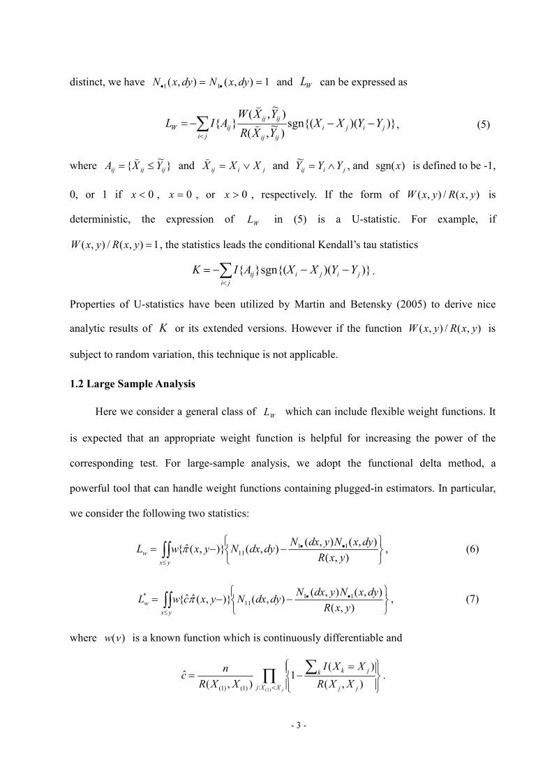
distinct, we have 1),(),( 11 == •• dyxNdyxN and WL can be expressed as
∑<
−−−=ji
jiji
ijij
ijij
ijW YYXXYXR
YXWAIL )})(sgn{(
)~,(
)~,(
}{ (
(
, (5)
where }~
{ ijijij YXA ≤=(
and jiij XXX ∨=(
and jiij YYY ∧=~
, and )sgn(x is defined to be -1,
0, or 1 if 0<x , 0=x , or 0>x , respectively. If the form of ),(/),( yxRyxW is
deterministic, the expression of WL in (5) is a U-statistic. For example, if
1),(/),( =yxRyxW , the statistics leads the conditional Kendall’s tau statistics
∑<
−−−=ji
jijiij YYXXAIK )})(sgn{(}{ .
Properties of U-statistics have been utilized by Martin and Betensky (2005) to derive nice
analytic results of K or its extended versions. However if the function ),(/),( yxRyxW is
subject to random variation, this technique is not applicable.
1.2 Large Sample Analysis
Here we consider a general class of WL which can include flexible weight functions. It
is expected that an appropriate weight function is helpful for increasing the power of the
corresponding test. For large-sample analysis, we adopt the functional delta method, a
powerful tool that can handle weight functions containing plugged-in estimators. In particular,
we consider the following two statistics:
∫∫≤
••
−−=yx
wyxR
dyxNydxNdydxNyxwL
),(
),(),(),()},(ˆ{ 11
11π , (6)
∫∫≤
••
−−=yx
wyxR
dyxNydxNdydxNyxcwL
),(
),(),(),()},(ˆˆ{ 11
11
* π , (7)
where )(vw is a known function which is continuously differentiable and
∏ ∑<
=−=
jXXj jj
k jk
XXR
XXI
XXR
nc
)1(:)1()1( ),(
)(1
),(ˆ .

- 4 -
Notice that wL and *
wL differ in whether the estimator c is involved. Also note that these
two statistics can be considered as approximations of the unbiased statistics
∫∫≤
••
−−yx
yxR
dyxNydxNdydxNyxw
),(
),(),(),()},({ 11
11π ,
∫∫≤
••
−−yx
yxR
dyxNydxNdydxNyxcw
),(
),(),(),()},({ 11
11π ,
respectively. The functional delta method can handle the extra estimation of the
hypothesized weight function in a systematic way.
To simplify the analysis we assume that the distributions of ),( YX under the null
hypothesis in (1) are absolutely continuous. The formula in (6) and (7) can be re-expressed as
the following functional forms:
∫∫ ∫∫ ∧≤∨−−
−∧∨−∧∨
−=**
*)*,(ˆ),(ˆ*)}*)(sgn{()**,(ˆ
)}**,(ˆ{
2 yyxxw yxdyxdyyxx
yyxx
yyxxwnL ππ
ππ
,
∫∫ ∫∫ ∧≤∨−−
−∧∨−∧∨
−=**
* *)*,(ˆ),(ˆ*)}*)(sgn{()**,(ˆ
)}**,(ˆ)ˆ({
2 yyxxw yxdyxdyyxx
yyxx
yyxxgwnL ππ
πππ
where )(⋅g is a functional satisfying )ˆ(ˆ πgc = defined in Appendix A.3. The proofs of the
above theoretical results are provided in the Appendices A.1 and A.3. Briefly speaking, these
functionals can be shown to be Hadamard differentiable functions of π given the
differentiability of )(⋅w . By applying the functional delta method (Van Der Vaart 1998, p. 297),
we obtain the following asymptotic expressions:
)1(),(2/12/1
P
j
jjw oYXUnLn +−= ∑−−,
)1(),(*2/1*2/1
P
j
jjw oYXUnLn +−= ∑−− ,
where ),( jj YXU and ),(* jj YXU are defined in Appendix A.1 and A.3.
Theorem 1: Under 0H , wLn 2/1− converges in distribution to a mean-zero normal random
variable with variance ]),([ 22
jj YXUE=σ where ),( jj YXU is defined in Appendix A.1.

- 5 -
Corollary 1: Under 0H , ρLn 2/1− , a special case of wLn 2/1− with ρvvw =)( converges in
distribution to a mean-zero normal random variable with variance ]),([ 2
jj YXUE ρ , where
*).*,()},(),({
*)}*)(sgn{()**,(
*)*,(),(*)}*)(sgn{()}**,(*)*,({
)**,(2/)1(
),(
**
1
**
2
yxdyxdyYxXI
yyxxyyxx
yxdyxdyyxxyyxxyyYxxXI
yyxx
YXU
ii
yyxx
jj
yyxx
jj
ππ
π
πππ
πρ
ρ
ρ
ρ
+==×
−−−∧∨−
−−−∧∨−∧≥∨≤×
−∧∨−=
∫∫ ∫∫
∫∫ ∫∫
∧≤∨
−
∧≤∨
−
An analytic variance estimator for the ρL class is presented in Section 4.
To study the statistics *
wL , we need to examine the property of c which is closely
related to the marginal estimators of )(tFX and )(tSY . Asymptotic normality of *
wL can be
established under the following condition.
Identifiability Assumption (I): There exists two positive numbers UL xy < such that
0)( >LX yF , 1)( =LY yS , 1)( =UX xF and 0)( >UY xS .
The above statement is an identifiability condition for ))(),(( ⋅⋅ YX SF , which has been routinely
used in theoretical analysis of truncation data. For example, the upper limit Ux plays the same
role as the notation *T in Wang et al. (1986). Assumption (I) also guarantees the condition
that nttR /),( is away from zero asymptotically (Chaieb et al., 2006) so that the denominator
terms ),( )1()1( XXR and ),( jj XXR for c is away from zero. Thus, under 0H and
Assumption (I), c is a reliable estimator of 0c .
Theorem 2: Under 0H and Assumption (I), *2/1
wLn− converges in distribution to a mean-zero
normal distribution with variance ]),([ 2*2
* jj YXUE=σ where ),(* jj YXU is defined in
Appendix A.3.
2. JACKKNIFE ESTIMATOR OF VARIANCE

- 6 -
The asymptotic variance of WL can be estimated by the jackknife estimator:
∑ ⋅− −−
i
W
i
W LLn
n 2)()( )(1
,
where )( i
WL−
has the form of WL without the i th observation and ∑ −⋅ =i
i
WW LnL )()( )/1( .
Asymptotic properties of the jackknife variance estimator are closely related to smoothness of
the corresponding functional expression. Specifically the test statistics wL in the class (6) can
be expressed as )ˆ(πΦ−n , where ),(ˆˆ yxππ = is an empirical process and )(⋅Φ is a
functional defined on a space of function )|,Pr(),( YXyYxXyx ≤>≤== ππ (see
Appendix A.1). In proving the asymptotic normality, we have shown that )(⋅Φ is Hadamard
differentiable with respect to the argument π . However, to show consistency of the jackknife
variance estimator, we need a more strict smoothness condition on )(⋅Φ called continuous
Gateaux differentiability (Shao 1993).
Theorem 3: Under 0H , the asymptotic variances 2σ for wL can be consistently estimated
by the jackknife method.
Theorem 4: Under 0H and Assumption (I), the asymptotic variances 2
*σ for *
wL can be
consistently estimated by the jackknife method.
The proofs of the above theorems are given in Appendix A.4.
3. LARGE SAMPLE PROPERITES UNDER CENSORING
3.1 The Proposed Test Statistics
When iY is further subject to censoring by iC , observed data become ),,{( iii ZX δ
)},...,1( ni = subject to ii ZX ≤ , where iii CYZ ∧= and )( iii CYI ≤=δ . Assume that iC
is independent of ),( ii YX . At an uncensored failure point ),( yx with yx ≤ , we use the
same notations for the cell and marginal counts with the following modified definitions:
∑ ====j
jjj yZxXIdydxN )1,,(),(11 δ , ∑ ≥==•j
jj yZxXIydxN ),(),(1 ,
- 7 -
∑ ==≤=•j
jjj yZxXIdyxN )1,,(),(1 δ and ∑ ≥≤=j
jj yZxXIyxR ),(),( .
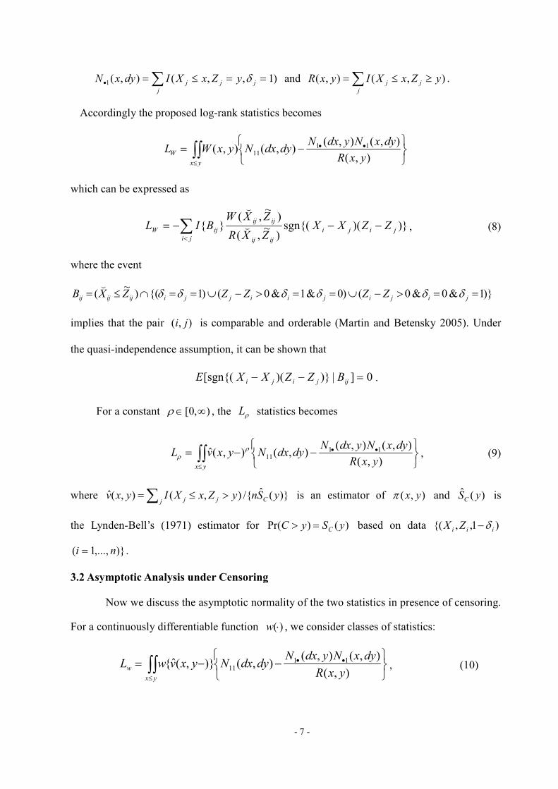
Accordingly the proposed log-rank statistics becomes
∫∫≤
••
−=yx
WyxR
dyxNydxNdydxNyxWL
),(
),(),(),(),( 11
11
which can be expressed as
∑<
−−−=ji
jiji
ijij
ijij
ijW ZZXXZXR
ZXWBIL )})(sgn{(
)~
,(
)~
,(}{ (
(
, (8)
where the event
)}1&0&0()0&1&0()1{()~
( ==>−∪==>−∪==∩≤= jijijiijjiijijij ZZZZZXB δδδδδδ(
implies that the pair ),( ji is comparable and orderable (Martin and Betensky 2005). Under
the quasi-independence assumption, it can be shown that
0]|)})([sgn{( =−− ijjiji BZZXXE .
For a constant ),0[ ∞∈ρ , the ρL statistics becomes
∫∫≤
••
−−=yx
yxR
dyxNydxNdydxNyxvL
),(
),(),(),(),(ˆ 11
11
ρρ , (9)
where ∑ >≤=j Cjj ySnyZxXIyxv )}(ˆ/{),(),(ˆ is an estimator of ),( yxπ and )(ˆ ySC is
the Lynden-Bell’s (1971) estimator for )()Pr( ySyC C=> based on data )1,,{( iii ZX δ−
)},...,1( ni = .
3.2 Asymptotic Analysis under Censoring
Now we discuss the asymptotic normality of the two statistics in presence of censoring.
For a continuously differentiable function )(⋅w , we consider classes of statistics:
∫∫≤
••
−−=yx
wyxR
dyxNydxNdydxNyxvwL
),(
),(),(),()},(ˆ{ 11
11 , (10)

- 8 -
∫∫≤
••
−−=yx
wyxR
dyxNydxNdydxNyxvcwL
),(
),(),(),()},(ˆˆ{ 11
11
**. (11)
where jjXX min)1( = and
∏ ∑<
=−=
jXXj jj
k jk
XXR
XXI
XXR
nc
)1(:)1()1(
*
),(
)(1
),(ˆ .
Asymptotic normality of the modified statistics is only briefly sketched in Appendix
A.5 since the related formula under censoring are too complicated and provide no new insight.
Define ncCyYxXIcyxHj jjj /),,(),,(ˆ ∑ >>≤= which is the empirical estimator of
)|,,Pr(),,( ZXcCyYxXcyxH ≤>>≤= . It follows that
*)*,*,(ˆ),,(ˆ*)}*)(sgn{(
)**,***,(ˆ
*)}**,;ˆ({
2 ***
cyxHdcyxHdyyxx
ccyyccyyxxH
ccyyxxHwnL
ccyyxxw
−−×
−∧∧∧−∧∧∧∨
∧∧∧∨−= ∫∫ ∫∫ ∫∫ ∫∫ ∧<∧≤∨
ϕ
,
*)*,*,(ˆ),,(ˆ*)}*)(sgn{(
)**,***,(ˆ
*)}**,;ˆ()ˆ({
2 ***
**
cyxHdcyxHdyyxx
ccyyccyyxxH
ccyyxxHHgwnL
ccyyxxw
−−×
−∧∧∧−∧∧∧∨
∧∧∧∨−= ∫∫ ∫∫ ∫∫ ∧<∧≤∨
ϕ,
where ),;( yx⋅ϕ and )(* ⋅g are functions such that ),;ˆ(),(ˆ yxHyx ϕν =− and )ˆ(ˆ ** Hgc = ,
each of which is defined in Appendix A.5. Asymptotic normality of wL and *
wL can be
established by applying the functional delta method based on the facts that both of them are
Hadamard differentiable functions of H and the process )ˆ(2/1 HHn − converges weakly to
a Gaussian process. Similar to the uncensored case, consistency of the jackknife variance
estimator is built based on the continuous Gateaux differentiability of the corresponding
functional expression. The proof is similar as that for Theorem 3 and 4 and hence is omitted.
4. EMPIRICAL VARIANCE AND JACKKNIFE VARIANCE ESTIMATOR
In absence of censoring, asymptotic variance of the ρL test defined in (4) has a
- 9 -
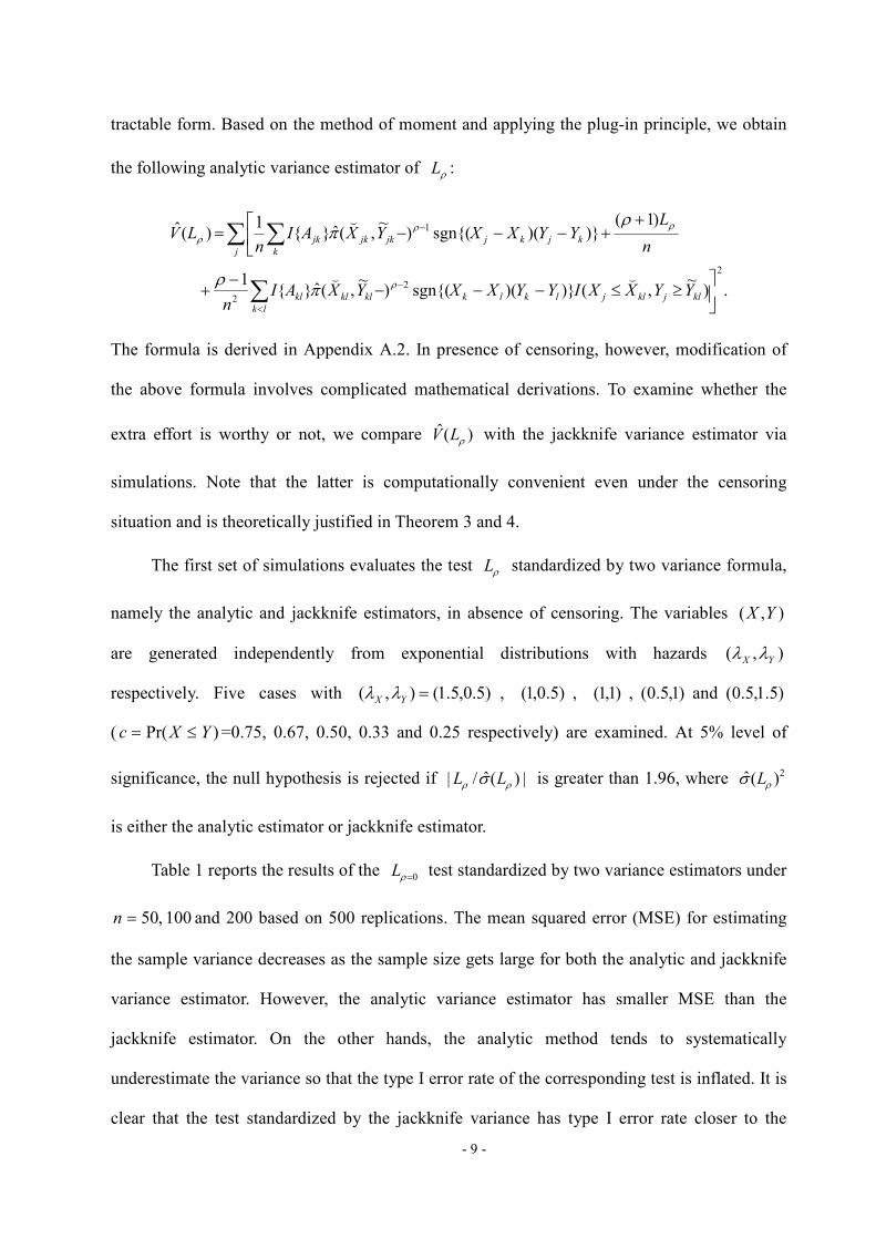
tractable form. Based on the method of moment and applying the plug-in principle, we obtain
the following analytic variance estimator of ρL :
.)~
,()})(sgn{()~,(ˆ}{
1
)1()})(sgn{()
~,(ˆ}{
1)(ˆ
2
2
2
1
≥≤−−−
−+
++
−−−=
∑
∑ ∑
<
−
−
lk
kljkljlklkklklkl
j k
kjkjjkjkjk
YYXXIYYXXYXAIn
n
LYYXXYXAI
nLV
((
(
ρ
ρρρ
πρ
ρπ
The formula is derived in Appendix A.2. In presence of censoring, however, modification of
the above formula involves complicated mathematical derivations. To examine whether the
extra effort is worthy or not, we compare )(ˆ ρLV with the jackknife variance estimator via
simulations. Note that the latter is computationally convenient even under the censoring
situation and is theoretically justified in Theorem 3 and 4.
The first set of simulations evaluates the test ρL standardized by two variance formula,
namely the analytic and jackknife estimators, in absence of censoring. The variables ),( YX
are generated independently from exponential distributions with hazards ),( YX λλ
respectively. Five cases with )5.0,5.1(),( =YX λλ , )5.0,1( , )1,1( , )1,5.0( and )5.1,5.0(
( )Pr( YXc ≤= =0.75, 0.67, 0.50, 0.33 and 0.25 respectively) are examined. At 5% level of
significance, the null hypothesis is rejected if |)(ˆ/| ρρ σ LL is greater than 1.96, where 2)(ˆ ρσ L
is either the analytic estimator or jackknife estimator.
Table 1 reports the results of the 0=ρL test standardized by two variance estimators under
100,50=n and 200 based on 500 replications. The mean squared error (MSE) for estimating
the sample variance decreases as the sample size gets large for both the analytic and jackknife
variance estimator. However, the analytic variance estimator has smaller MSE than the
jackknife estimator. On the other hands, the analytic method tends to systematically
underestimate the variance so that the type I error rate of the corresponding test is inflated. It is
clear that the test standardized by the jackknife variance has type I error rate closer to the

- 10 -
nominal 5% level in all the cases. Table 2 summarizes the results of the 1=ρL test. Both
variance estimators tend to overestimate the true variance but the jackknife estimator has
slightly smaller MSE and still produces more accurate type I error probability than the analytic
estimator. The results indicate that the test standardized by the jackknife variance estimator has
more reliable performance in most situations.
The second set of simulations evaluates the test WL standardized by the jackknife
variance estimator in presence of censoring in which the analytic formula is not available.
Three independent variables ),,( CYX are generated from exponential distributions with
hazard rates ),,( CYX λλλ =(1.5, 1.0, 0.5) respectively yielding )(* ZXPc ≤= =0.5. Table 3
summarizes the results for three tests 0=ρL , 1=ρL and loginvL under =n 50, 100 and 200
based on 500 replications. The jackknife variance method, on the average, is quite accurate.
The MSE for estimating the variance gets small as the number of sample increases.
Furthermore the type I error rates for the three statistics are all close to the nominal level.
5. CONCLUSION
To establish asymptotic normality, we apply the functional delta method which can
handle more general forms of statistics than the approaches based on U-statistics or rank
statistics. The expression of the proposed statistics as a statistically differentiable functional
allows us to derive an analytic variance estimator and justify the use of the jackknife method in
variance estimation. Simulation analysis indicates that the jackknife method is a better
alternative because its convenience and reliable results. Nevertheless one may try to modify the
analytic variance formula by including more omitted terms in the Taylor expansion to see if the
bias can be reduced. However the derivations will be very tedious and may not be worthy from
a practical point of view.

- 11 -
APPENDIX: ASYMPTOTIC ANALYSIS
Let }),0{[ 2∞D and )},0{[ ∞D be the collection of all right-continuous functions
with left-side limit defined on 2),0[ ∞ and ),0[ ∞ respectively, under which the norms are
defined by |),(|sup),( , yxfyxf yx=∞
for }),0{[ 2∞∈Df and |)(|sup)( xfxf x=∞
for )},0{[ ∞∈Df . We assume that the function 0/)()(),( cySxFyx YX=π is absolutely
continuous. Hereafter, expectation symbols represent the conditional expectation given
YX ≤ . The notation )1(Po is short of random variables that converge to zero in
probability, under the conditional probability induced by 0/)()(),( cySxFyx YX=π . The
empirical process on the plane is defined as:
∑ >≤=j
jj yYxXIn
yx ),(1
),(π .
It can be shown that )),(),(ˆ(2/1 yxyxn ππ − converges weakly to a mean 0 Gaussian
process ),( yxV on }),0{[ 2∞D with the covariance given by
),(),(),()},(),,({ 221121212211 yxyxyyxxyxVyxVCov πππ −∨∧= ,
for any ),( 11 yx , 2
22 ),0[),( ∞∈yx .
A.1 Proof of Theorem 1
By some algebraic manipulations, the statistic wL in (6) can be expressed in terms of
the weighted sum of signs such that
∫∫≤
••
−−=yx
wyxR
dyxNydxNdydxNyxwL
),(
),(),(),()},(ˆ{ 11
11π
,)})(sgn{()
~,(ˆ
)}~,(ˆ{
}{2
1
)})(sgn{()
~,(ˆ
)}~,(ˆ{
}{1
)})(sgn{()
~,(
)}~,(ˆ{
}{
,
∑
∑
∑
−−−
−−=
−−−
−−=
−−−
−=
<
<
ji
jiji
ijij
ijij
ij
ji
jiji
ijij
ijij
ij
ji
jiji
ijij
ijij
ij
YYXXYX
YXwAI
n
YYXXYX
YXwAI
n
YYXXYXR
YXwAI
(
(
(
(
(
(
π
π
π
π
π

- 12 -
where the last equation use the facts that each term is symmetric for indices ),( ji and
),( ij and that 0)})(sgn{( =−− jjjj YYXX . Using the property that
iyYxXnyxd
ii somefor
otherwise
,
0
/1),(ˆ
==−
=π ,
the above expression can be written as
),ˆ(
*)*,(ˆ),(ˆ*)}*)(sgn{()**,(ˆ
)}**,(ˆ{
2 **
π
ππππ
Φ−≡
−−−∧∨−∧∨
−= ∫∫ ∫∫ ∧≤∨
n
yxdyxdyyxxyyxx
yyxxwnL
yyxxw
where the definition of the functional R→∞⋅Φ }),0{[:)( 2D is given by
∫∫∫∫ ∧≤∨−−
−∧∨−∧∨
=Φ**
*)*,(),(*)}*)(sgn{()**,(2
)}**,({)(
yyxxyxdyxdyyxx
yyxx
yyxxwππ
ππ
π .
The argument }),0{[ 2∞∈Dπ in the preceding equation does not need to be
0/)()(),( cySxFyx YX=π , but if so, the above integral can be interpreted as an expectation
under quasi-independence. It can be shown that 0)( =Φ π since
,}~,|)})({sgn{(
)~,(2
)}~,({
}{
)})(sgn{()
~,(2
)}~,({
}{)(
12122121
1212
121212
2121
1212
121212
−−
−
−=
−−
−
−=Φ
YXYYXXEYX
YXwAIE
YYXXYX
YXwAIE
((
(
(
(
ππ
ππ
π
and
0}~,|)})({sgn{( 12122121 ===−− yYxXYYXXE
( for yx ≤ .
Here, the last equation follows from Chaieb et al. (2006). The basic idea of the functional
delta method is to find the asymptotic behavior of )ˆ(πΦ through a differential analysis of
)(πΦ in a neighborhood of 0/)()(),( cySxFyx YX=π . A first order expansion would have
the form:
)ˆ()()ˆ()ˆ( πππππ π −Φ′≈Φ−Φ=Φ .
where )(⋅Φ′π will be rigorously defined later. The analysis turn the weak convergence of
)ˆ(πΦ into the weak convergence of ππ −ˆ , which will next be further investigated in a

- 13 -
rigorous fashion.
By direct calculations, we can prove the Hadamard differentiability of )(⋅Φ . The
linearly differentiable map of )(⋅Φ at arbitrary argument }),0{[ 2∞∈Dπ with direction
}),0{[ 2∞∈Dh is:
∫∫∫∫
∫∫∫∫
∫∫∫∫
∧≤∨
∧≤∨
∧≤∨
−−−∧∨−∧∨
+
−−−∧∨−∧∨−∧∨
−
−−−∧∨−∧∨−∧∨′
=
Φ′
yyxx
yyxx
yyxx
yxdyxdhyyxxyyxx
yyxxw
yxdyxdyyxxyyxxhyyxx
yyxxw
yxdyxdyyxxyyxxhyyxx
yyxxw
h
*
* 2
*
*)*,(),(*)}*)(sgn{()**,(
)}**,({
*)*,(),(*)}*)(sgn{()**,()**,(2
)}**,({
*)*,(),(*)}*)(sgn{()**,()**,(2
)}**,({
)(
πππ
ππππ
ππππ
π
,
where uuwuw ∂∂=′ /)()( . By applying the functional delta method (Van Der Vaart 1998, p.
297), we obtain the following asymptotic linear expression:
),1()(
)1()}ˆ({
)}()ˆ({
)ˆ(
),(
2/1
2/1
2/1
2/12/1
P
j
YX
P
w
on
on
n
nLn
jj+−Φ′−=
+−Φ′−=
Φ−Φ−=
Φ−=
∑−
−
πδ
ππ
ππ
π
π
π
where ),(),(),( yYxXIyx jjYX jj>≤=δ . It is easy to see that the sequences,
)(),( ),( πδπ −Φ′≡jj YXjj YXU for nj ,,1K= ,
are iid random variables with 0)],([ =jj YXUE at 0/)()(),( cySxFyx YX=π since
0)0(
])[()]([ ),(),(
=Φ′=
−Φ′=−Φ′
π
ππ πδπδjjjj YXYX EE
.
Based on the central limit theorem, wLn 2/1− converges in distribution to a mean 0 normal
random variable with variance ]),([ 22
jj YXUE=σ .
A.2 Analytic Variance Estimator for the ρL Test
The ρL statistics forms a nice subset of wL such that 2σ can be expressed by

- 14 -
analytic formula. The functional expression has the form ),ˆ(πρ Φ−= nL where
∫∫∫∫ ∧≤∨
− −−−∧∨=Φ**
1 *)*,(),(*)}*)(sgn{()**,()2/1()(yyxx
yxdyxdyyxxyyxx ππππ ρ
for }),0{[ 2∞∈Dπ and 0)( =Φ π for 0/)()(),( cySxFyx YX=π . Specifically, the
corresponding derivative map is given by
∫∫∫∫
∫∫∫∫
∧≤∨
−
∧≤∨
−
−−−∧∨+
−−−∧∨−∧∨−=
Φ′
.*)*,(),(*)}*)(sgn{()**,(
*)*,(),(*)}*)(sgn{()**,()**,(2/)1(
)(
**
1
**
2
yyxx
yyxx
yxdyxdhyyxxyyxx
yxdyxdyyxxyyxxhyyxx
h
ππ
πππρ
ρ
ρ
π
The variance ]),([ 22
jj YXUE=σ can be estimated by nj YX jj
/)ˆ(2
),(ˆ∑ −Φ′ πδπ , where
*)*,(ˆ)},(ˆ),({
*)}*)(sgn{()**,(ˆ
*)*,(ˆ),(ˆ*)}*)(sgn{()}**,(ˆ*)*,({
)**,(ˆ2/)1(
)ˆ(
**
1
**
2
),(ˆ
yxdyxdyYxXI
yyxxyyxx
yxdyxdyyxxyyxxyyYxxXI
yyxx
jj
yyxx
jj
yyxx
YX jj
ππ
π
πππ
πρ
πδ
ρ
ρ
π
+==×
−−−∧∨−
−−−∧∨−∧≥∨≤×
−∧∨−=
−Φ′
∫∫∫∫
∫∫∫∫
∧≤∨
−
∧≤∨
−
.
Turning the integral to the double summation, we obtain
.)})(sgn{()~,(ˆ}{
2
)})(sgn{()~,(ˆ}{
1
)})(sgn{()~,(ˆ}{
1
)~
,()})(sgn{()~,(ˆ}{
1)ˆ(
1
2
1
1
2
2
2),(ˆ
∑
∑
∑
∑
<
−
−
<
−
<
−
−−−−
−−−+
−−−−
−
≥≤−−−−
=−Φ′
lk
lklkklklkl
k
kjkjjkjkjk
lk
lklkklklkl
lk
kljkljlklkklklklYX
YYXXYXAIn
YYXXYXAIn
YYXXYXAIn
YYXXIYYXXYXAInjj
ρ
ρ
ρ
ρπ
π
π
πρ
πρ
πδ
(
(
(
((
The second and fourth terms combine to form nL /)1( ρρ + . Thus we get
.)~
,()})(sgn{()~,(ˆ}{
1
)1()})(sgn{()
~,(ˆ}{
1)ˆ(
2
2
1
),(ˆ
∑
∑
<
−
−
≥≤−−−−
+
++−−−=−Φ′
lk
kljkljlklkklklkl
k
kjkjjkjkjkYX
YYXXIYYXXYXAIn
n
LYYXXYXAI
njj
((
(
ρ
ρρπ
πρ
ρππδ

- 15 -
Based on the above expressions, we can estimate 2)( σρ nLAVar = by the following
empirical estimator:
.)~
,()})(sgn{()~,(ˆ}{
1
)1()})(sgn{()
~,(ˆ}{
1ˆ
2
2
2
12
≥≤−−−
−+
++
−−−=
∑
∑ ∑
<
−
−
lk
kljkljlklkklklkl
j k
kjkjjkjkjk
YYXXIYYXXYXAIn
n
LYYXXYXAI
nn
((
(
ρ
ρρ
πρ
ρπσ
A.3 Proof of Theorem 2
The statistic *
wL involves c which is the estimator of the normalizing constant 0c .
From the result of He and Yang (1998), c can be written as
∫∞
=0
)(ˆ)(ˆˆ uFduSc XY ,
where ∏<
−−=
ut
Xuu
udtF
),(ˆ
)0,(ˆ1)(ˆ
ππ
and ∏≤
−∞
+=tu
Yuu
udtS
),(ˆ
),(ˆ1)(ˆ
ππ
are the product limit
estimators of )Pr( tX ≤ and )Pr( tY > respectively (Lynden-Bell 1971). Define
)ˆ(ˆ πgc = and we will show that the map cg ˆˆ: aπ is the composition of two Hadamard
differentiable maps:
∫∞
0)(ˆ)(ˆ))(ˆ),(ˆ(),(ˆ uFduSySxFyx XYYX aaπ . (A.1)
It is well-known for right-censored data that the product limit estimator is Hadamard
differentiable function of the corresponding empirical processes. For truncation data, we
apply the arguments of Example 20.15 in Van Der Vaart (1998) to show the Hadamard
differentiability of the maps from }),0{[ 2∞D to )},0{[ ∞D :
)(ˆ),(ˆ tFyx Xaπ , )(ˆ),(ˆ tSyx Yaπ .
To prove the former statement, we decompose each map into three differentiable maps. For
example, one can write
- 16 -
,)}(ˆ1{)(ˆ
),(ˆ
)0,(ˆ)(ˆ)),(ˆ/1),0,(ˆ(),(ˆ
0
∏
∫
<Λ−=
−=Λ−
ut XX
t
X
udtF
uu
udtxxxyx
a
aaππ
πππ
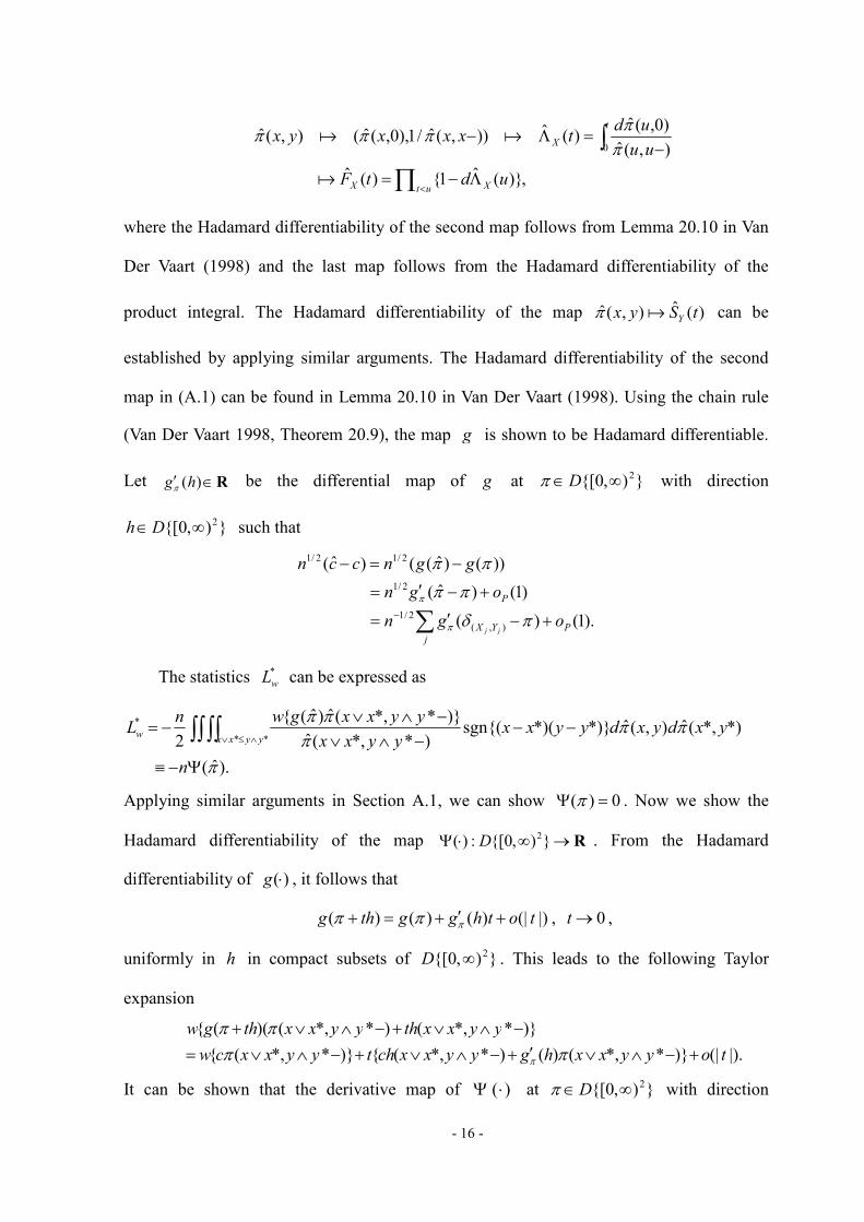
where the Hadamard differentiability of the second map follows from Lemma 20.10 in Van
Der Vaart (1998) and the last map follows from the Hadamard differentiability of the
product integral. The Hadamard differentiability of the map )(ˆ),(ˆ tSyx Yaπ can be
established by applying similar arguments. The Hadamard differentiability of the second
map in (A.1) can be found in Lemma 20.10 in Van Der Vaart (1998). Using the chain rule
(Van Der Vaart 1998, Theorem 20.9), the map g is shown to be Hadamard differentiable.
Let R∈′ )(hgπ be the differential map of g at }),0{[ 2∞∈Dπ with direction
}),0{[ 2∞∈Dh such that
).1()(
)1()ˆ(
))()ˆ(()ˆ(
),(
2/1
2/1
2/12/1
P
j
YX
P
ogn
ogn
ggnccn
jj+−′=
+−′=
−=−
∑− πδ
ππ
ππ
π
π
The statistics *
wL can be expressed as
).ˆ(
*)*,(ˆ),(ˆ*)}*)(sgn{()**,(ˆ
)}**,(ˆ)ˆ({
2 **
*
π
πππ
ππ
Ψ−≡
−−−∧∨
−∧∨−= ∫∫∫∫ ∧≤∨
n
yxdyxdyyxxyyxx
yyxxgwnL
yyxxw
Applying similar arguments in Section A.1, we can show 0)( =Ψ π . Now we show the
Hadamard differentiability of the map R→∞⋅Ψ }),0{[:)( 2D . From the Hadamard
differentiability of )(⋅g , it follows that
|)(|)()()( tothggthg +′+=+ πππ , 0→t ,
uniformly in h in compact subsets of }),0{[ 2∞D . This leads to the following Taylor
expansion
|).(|)}**,()()**,({)}**,({
)}**,()**,()(({
toyyxxhgyyxxchtyyxxcw
yyxxthyyxxthgw
+−∧∨′+−∧∨+−∧∨=
−∧∨+−∧∨+
ππππ
π
It can be shown that the derivative map of )( ⋅Ψ at }),0{[ 2∞∈Dπ with direction

- 17 -
}),0{[ 2∞∈Dh can be written as
.*)*,(),(*)}*)(sgn{()**,(
)}**,({
*)*,(),(*)}*)(sgn{()**,()**,(2
)}**,()({
*)*,(),(*)}*)(sgn{(2
)}**,({)(
*)*,(),(*)}*)(sgn{()**,()**,(2
)}**,({)(
)(
*
* 2
*
*
∫∫∫∫
∫∫∫∫
∫∫∫∫
∫∫∫∫
∧≤∨
∧≤∨
∧≤∨
∧≤∨
−−−∧∨−∧∨
+
−−−∧∨−∧∨−∧∨
−
−−−∧∨′′
+
−−−∧∨−∧∨−∧∨′
=
Ψ′
yyxx
yyxx
yyxx
yyxx
yxdyxdhyyxxyyxx
yyxxw
yxdyxdyyxxyyxxhyyxx
yyxxgw
yxdyxdyyxxyyxxwhg
yxdyxdyyxxyyxxhyyxx
yyxxwg
h
πππ
πππππ
πππ
πππππ
π
π
By applying the functional delta method, we obtain the following asymptotic linear
expressions:
)ˆ(2/1*2/1 πΨ−=− nLn w )}()ˆ({2/1 ππ Ψ−Ψ−= n
),1()( ),(
2/1
P
j
YX onjj
+−Ψ′−= ∑− πδπ
where the sequences,
)(),( ),(
* πδπ −Ψ′≡jj YXjj YXU ),,1( nj K= ,
are mean 0 i.i.d. random variables. From the central limit theorem, *2/1
wLn− converges
weakly to a mean 0 normal distribution with the variance ]),([ 2*2
* jj YXUE=σ .
A.4 Consistency of the Jackknife Estimator
We have shown that wLn 2/1− is asymptotically normal with a finite variance. Now we
show consistency of the jackknife variance estimator of wL . According to Theorem 3.1 of
Shao (1993), we need to show the continuous Gateaux differentiability of )(πΦ at
}),0{[ 2∞∈Dπ . Note that the Hadamard differentiability is stronger than the Gateaux
differentiability and hence the Gateaux derivative map is given by )(hπΦ′ , available from
Section A.1. We only need to show the continuous requirement of the derivative map. For
sequence }),0{[ 2∞∈Dkπ satisfying 0→−∞
ππ k and 0→kt for K,2,1=k , we need
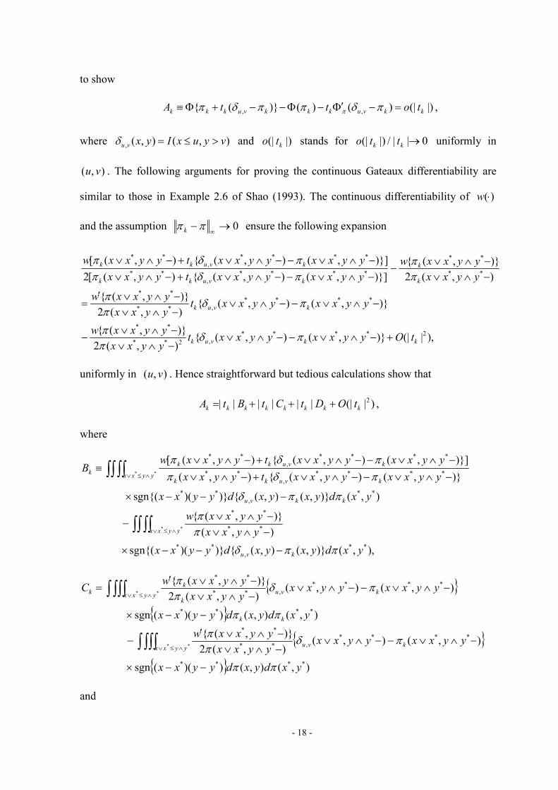
- 18 -
to show
|)(|)()()}({ ,, kkvukkkvukkk tottA =−Φ′−Φ−−+Φ≡ πδππδπ π ,
where ),(),(, vyuxIyxvu >≤=δ and |)(| kto stands for 0||/|)(| →kk tto uniformly in
),( vu . The following arguments for proving the continuous Gateaux differentiability are
similar to those in Example 2.6 of Shao (1993). The continuous differentiability of )(⋅w
and the assumption 0→−∞
ππ k ensure the following expansion
),|(|)},(),({),(2
)},({
)},(),({),(2
)},({
),(2
)},({
)}],(),({),([2
)}],(),({),([
2****
,2**
**
****
,**
**
**
**
****
,
**
****
,
**
kkvuk
kvuk
k
k
kvukk
kvukk
tOyyxxyyxxtyyxx
yyxxw
yyxxyyxxtyyxx
yyxxw
yyxx
yyxxw
yyxxyyxxtyyxx
yyxxyyxxtyyxxw
+−∧∨−−∧∨−∧∨−∧∨
−
−∧∨−−∧∨−∧∨−∧∨′
=
−∧∨−∧∨
−−∧∨−−∧∨+−∧∨
−∧∨−−∧∨+−∧∨
πδππ
πδππ
ππ
πδππδπ
uniformly in ),( vu . Hence straightforward but tedious calculations show that
)|(||||||| 2
kkkkkkkk tODtCtBtA +++= ,
where
,),()},(),({)})(sgn{(
),(
)},({
),()},(),({)})(sgn{(
)},(),({),(
)}],(),({),([
**
,
**
**
**
**
,
**
****
,
**
****
,
**
**
**
yxdyxyxdyyxx
yyxx
yyxxw
yxdyxyxdyyxx
yyxxyyxxtyyxx
yyxxyyxxtyyxxwB
kvu
yyxx
kkvu
yyxxkvukk
kvukk
k
ππδ
ππ
ππδ
πδπ
πδπ
−−−×
−∧∨−∧∨
−
−−−×
−∧∨−−∧∨+−∧∨
−∧∨−−∧∨+−∧∨≡
∫∫ ∫∫
∫∫ ∫∫
∧≤∨
∧≤∨
{ }
{ }{ }
{ } ),(),())((sgn
),(),(),(2
)},({
),(),())((sgn
),(),(),(2
)},({
****
****
,**
**
****
****
,**
**
**
**
yxdyxdyyxx
yyxxyyxxyyxx
yyxxw
yxdyxdyyxx
yyxxyyxxyyxx
yyxxwC
kvuyyxx
kk
kvuyyxx
k
kk
ππ
πδππ
ππ
πδππ
−−×
−∧∨−−∧∨−∧∨−∧∨′
−
−−×
−∧∨−−∧∨−∧∨−∧∨′
=
∫ ∫∫∫
∫ ∫∫∫
∧≤∨
∧≤∨
and

- 19 -
).,(),()})(sgn{(
)},(),({),(2
)},({
),(),()})(sgn{(
)},(),({),(2
)},({
****
****
,2**
**
****
****
,2**
**
**
**
yxdyxdyyxx
yyxxyyxxyyxx
yyxxw
yxdyxdyyxx
yyxxyyxxyyxx
yyxxwD
yyxxkvu
kk
yyxxkvu
l
kk
ππ
πδππ
ππ
πδππ
−−×
−∧∨−−∧∨−∧∨−∧∨
−
−−×
−∧∨−−∧∨−∧∨−∧∨
≡
∫∫ ∫∫
∫∫ ∫∫
∧≤∨
∧≤∨
Under the assumption that 0→−∞
ππ k , it can be seen that kB kC and kD have order
)1(o . This proves the theorem 3.
To show the consistency of the jackknife variance estimator for *
wL stated in theorem
4, we only need to check whether the continuity of the Gateaux differential map of )(πΨ
which is available in Section A.3. The continuity requirement for the Gateaux differentiable
map )(hπΨ′ in Section A.3 can be verified after tedious algebraic operations similar to the
above arguments.
A.5 Asymptotic Analysis in Presence of Censoring
Based on the product integral form of the Lynden-Bell’s estimator )(ˆ ySC , we obtain
the expression
),;ˆ(}),,(ˆ),,(ˆ1{
),,(ˆ),(ˆ yxH
uuuHduuuH
yyxHyx
yu
ϕν ≡−−+
−−=−∏≤
. (A.2)
By some algebraic work, the event ijB can be written as )~~
(}{ ijijijij CYXIBI <≤=(
.
Then, we obtain the following functional expression:
∑
∑∫∫
−−−∧−∧
∧<≤×−=
−∆=
−−=<≤
••
ji
jiji
ijijijijij
ijijij
ijijij
ji
ij
ijij
ijij
ij
yx
w
YYXXCYCYXH
CYXHwCYXI
n
n
ZXR
ZXHwBI
yxR
dyxNydxNdydxNyxvwL
,2
1111
)})(sgn{()
~~,
~~,(ˆ
)}~~
,;ˆ({}
~~{
1
2
2
1
)~
,(
)}~
,;ˆ({2}{
),(
),(),(),()},(ˆ{
(
((
(
(
ϕ
ϕ

- 20 -
*)*,*,(ˆ),,(ˆ*)}*)(sgn{(
)**,***,(ˆ
*)}**,;ˆ({
2 ***
cyxHdcyxHdyyxx
ccyyccyyxxH
ccyyxxHwn
ccyyxx
−−×
−∧∧∧−∧∧∧∨
∧∧∧∨−= ∫∫ ∫∫ ∫∫ ∧<∧≤∨
ϕ.
Here, the last equation follows from the property
===
=otherwise
somefor,,
0
/1),,(ˆ
jcCyYxXncyxHd
jjj.
Based on similar arguments with Section A3, we can express the estimator *c as a function
of H such that )ˆ(ˆ ** Hgc = . Similar algebraic operations can be applied to obtain the
functional expression of *
wL .
- 21 -
REFERENCES
Chaieb, L. Rivest, L.-P. and Abdous, B. (2006), “Estimating Survival Under a Dependent
Truncation,” Biometrika, 93, 655-669.
Harrington, D. P., and Fleming, T. R. (1982), “A Class of Rank Test Procedures for
Censored Survival Data,” Biometrika, 69, 133-143.
He, S. and Yang, G. L. (1998), “Estimation of the Truncation Probability in the Random
Truncation Model,” Annals of Statistics. 26, 1011-1027.
Lynden-Bell, D. (1971), “A Method of Allowing for Known Observational Selection in
Small Samples Applied to 3RC Quasars,” Mon. Nat. R. Astr. Soc.,155, 95-118.
Martin, E. C. and Betensky, R. A. (2005), “Testing Quasi-independence of Failure and
Truncation via Conditional Kendall’s Tau,” Journal of the American Statistical
Association, 100, 484-492.
Shao, J. (1993), “Differentiability of Statistical Functionals and Consistency of the
Jackknife,” The Annals of Statistics, 21, 61-75.
Tsai, W. -Y. (1990), “Testing the Association of Independence of Truncation Time and
Failure Time,” Biometrika, 77, 169-177.
Van Der Vaart. A. W. (1998), “Asymptotic Statistics,” Cambridge Series in Statistics and
Probabilistic Mathematics, Cambridge: Cambridge University Press.
Wang, M. C., Jewell, N. P. and Tsai, W. Y. (1986), “Asymptotic Properties of the
Product-limit Estimate and Right Censored Data,” Annals of Statistic, 13, 1597-1605.

- 22 -
Table 1. Comparison of two (jackknife vs. analytic) variance estimators of
0
2/1
=−
ρLn in absence of censoring when 500 replications for pairs
X and Y are generated from independent exponential distributions
)Pr( YX
c
≤
=
n
Variance of
0
2/1
=−
ρLn
Average (MSE) of
the variance estimators Type I error (5%)
Jackknife Analytic Jackknife Analytic
0.75 50 0.819 0.870 (0.146) 0.653 (0.077) 0.048 0.092
100 0.872 0.955 (0.121) 0.786 (0.054) 0.062 0.078
200 0.930 0.997 (0.081) 0.875 (0.039) 0.066 0.078
0.67 50 0.735 0.885 (0.188) 0.652 (0.059) 0.058 0.084
100 0.859 0.941 (0.110) 0.774 (0.051) 0.062 0.074
200 0.923 0.957 (0.065) 0.846 (0.039) 0.064 0.072
0.50 50 0.688 0.872 (0.194) 0.630 (0.056) 0.048 0.068
100 0.820 0.943 (0.146) 0.762 (0.053) 0.056 0.076
200 0.814 0.981 (0.118) 0.851 (0.043) 0.048 0.056
0.33 50 0.723 0.897 (0.231) 0.630 (0.071) 0.044 0.078
100 0.733 0.931 (0.172) 0.738 (0.052) 0.050 0.064
200 0.837 0.941 (0.092) 0.815 (0.039) 0.050 0.064
0.25 50 0.696 0.852 (0.163) 0.604 (0.053) 0.046 0.062
100 0.802 0.903 (0.123) 0.720 (0.053) 0.064 0.082
200 0.896 0.960 (0.100) 0.825 (0.050) 0.052 0.066

- 23 -
Table 2. Comparison of two (jackknife vs. analytic) variance estimators of
1
2/1
=−
ρLn in absence of censoring when 500 replications for pairs of X and Y are
generated from independent exponential distributions
)Pr( YX
c
≤
=
n
Variance of
1
2/1
=−
ρLn
( 100× )
Average (MSE) of
the variance estimators
( 100× )
Type I error (5%)
Jackknife Analytic Jackknife Analytic
0.75 50 7.493 7.468 (0.0263) 7.604 (0.0264) 0.058 0.036
100 7.037 7.072 (0.0110) 7.159 (0.0118) 0.048 0.040
200 6.794 6.800 (0.0055) 6.850 (0.0057) 0.062 0.056
0.67 50 5.438 6.553 (0.0366) 6.614 (0.0377) 0.036 0.026
100 5.935 6.194 (0.0115) 6.263 (0.0119) 0.056 0.042
200 5.616 5.889 (0.0062) 5.928 (0.0065) 0.056 0.040
0.50 50 4.097 5.321 (0.0330) 5.352 (0.0340) 0.028 0.014
100 4.487 4.917 (0.0094) 4.964 (0.0101) 0.050 0.040
200 4.086 4.665 (0.0074) 4.689 (0.0077) 0.044 0.038
0.33 50 3.901 4.369 (0.0157) 4.426 (0.0168) 0.038 0.024
100 3.454 3.981 (0.0098) 4.015 (0.0103) 0.038 0.032
200 3.481 3.756 (0.0042) 3.779 (0.0044) 0.034 0.030
0.25 50 3.414 4.085 (0.0190) 4.124 (0.0203) 0.036 0.024
100 3.336 3.624 (0.0068) 3.660 (0.0073) 0.040 0.034
200 3.334 3.376 (0.0027) 3.400 (0.0028) 0.046 0.042

- 24 -
Table 3. Performance of WLn 2/1− standardized by the jackknife variance estimator
in absence of censoring when 500 replications for pairs X , Y and C are generated
from independent exponential distributions
Test statistics n
Variance of
WLn 2/1−
Average (MSE) of
the jackknife
variance estimator
Type I error (5%)
0
2/1
=−
ρLn 50 0.4678 0.5858 (0.06398) 0.050
100 0.5205 0.6142 (0.04585) 0.046
200 0.5828 0.6461 (0.02702) 0.050
1
2/1
=−
ρLn 50 0.0745 0.0777 (0.00103) 0.050
100 0.0720 0.0710 (0.00036) 0.052
200 0.0613 0.0658 (0.00020) 0.054
log
2/1
invLn− 50 0.2075 0.2560 (0.01580) 0.038
100 0.2382 0.2342 (0.00402) 0.052
200 0.2010 0.2190 (0.00253) 0.050