The Variance of Spectral Estimates - NASA · Technical Report No. 32-892 The Variance of Spectral Estimates Eugene R. Rodemich Richard M. Goldstein, Manager Communications Systems

I r .. ." .": ., -. .

- * I <,: h .

N A T I O N A L A E R O N A U T I C S A N D S P A C E A D M I N I S T R A T I O N . ._ . *.> ,, - ,L ..

* - -. L .. * .-- * . I .

- 1 *

Technical Report No. .32-892

The Variance of Spectral Estimates

Eugene R. Rodemich

. -

C-ALWORNIX t P i s r r ~ u r ~ OF TECHNOLOGY PASADENA, CALIFORNIA

March 31, 1966

https://ntrs.nasa.gov/search.jsp?R=19660016085 2018-09-22T05:27:56+00:00Z

, '

Technical Report No. 32-892

The Variance of Spectral Estimates

Eugene R. Rodemich

Richard M. Goldstein, Manager Communications Systems Research Section

J E T PROPULSION L A B O R A T O R Y CALIFORNIA 1NSTlTUTE O F TECHNOLOGY

P A S A D EN A, C A L I FOR N I A

March 3 1, 1966

Copyright 0 1966 Jet Propulsion Laboratory

California Institute of Technology

Prepared Under Contract No. NAS 7-100 National Aeronautics & Space Administration

JPL TECHNICAL REPORT NO . 32-892

CONTENTS

1 . Introduction . . . . . . . . . . . . . . . . . . . . . 1

II . Estimates for the Moments of &&) . . . . . . . . . . . 2

111 . The Means of Functions of the @v(kl . . . . . . . . . . . 10

IV . TheMainTheorem . . . . . . . . . . . . . . . . . . 15

V . The Value of F'(0) . . . . . . . . . . . . . . . . . . . u)

References . . . . . . . . . . . . . . . . . . . . . . . 21

Figure 1 . The function F (z) when y (XI takes four values with a ratio of 1:4 . . . . . . . . . . . . . . . . 21

' .

In this Report the main result proved is a generalization of a formula of Goldstein (Ref. I ) , who showed that if the estimate s^( 0 ) for the spectral density is computed by the use of the function y ( x ) = sgn( z), and if the spectrum is flat, then the dominant term in the variance of s (̂o) is W 1~' K I N . Theorem 3 evaluates this term for non-flat spectra and for more general functions y ( x ) .

This analysis shows that the loss in accuracy caused by working with y ( x ) instead of with x itself can be decreased considerably by using, for y( x ) , a step function with more than two values.

1. INTRODUCTION

The spectral density S (o), 10 I L r, of a discrete stationary Gaussian process { x k } , - 00 < k < 00, of mean

A simple choice of fi, (k) is zero, can be expressed in terms of the correlations R= (k) = E ( x n x n + k ) by

a

S (0) = Z eib R, (k) = R, (0) + 2 Z cos k0 R, (k). 00 where N is large. Each term in the sum has the expected

value R,(k) and the variance of this expression ap- proaches zero as N 3 co. Hence, for large N, the value

ability. However, for large N the evaluation of the sum can be quite time-consuming.

k = - a k = 1

An estimate of S (") can be obtained from observations of of this expression is to R z (kh with a high Prob- { x k } by --ting the series and replacing the quantities R,(k) with appropriate estimates &(k). If we assume that R,(O) = E(rQ is known, then the xLIs can be normalized so that R, (0) = 1, and the estimate for S (0 ) is It has been observed (Ref. 1) that if

1

JPL TECHNICAL REPORT NO. 32-892

then R, ( k ) = E ( y , ~ ~ + ~ ) satisfies the relation

R,(k) = sin[$R.(k)].

This suggests using

(3)

For large N, and for K small compared with N, this formula for 8,(k) can bz evaluated much more rapidly than (2) (Ref. 1). When S (a) is evaluated by (1) and (3), the problem of estimating its mean and variance arises. It is hoped that the mean is close to S ( 0 ) and the variance is small.

A more general method is considered here. We take y i = y ( x i ) , where y ( x ) is any odd, bounded, nondecreasing function, normalized so that E ( y ? ) = 1. It is shown by Lemma 3 that there is a function F ( t ) such that

In general, F ( t ) is not an entire function, but is analytic in a region of the complex plane including the open

interval - 1 < t < 1. For the present purposes, F (t) may be extended in any way to a continuous function on - 03 < t < 03. We take

With this definition, it is shown (Theorem 3) that, except for a term of the order 1/N, E [S (o)] is

and E {g (w)’} is approximately SK (o)*, with a leading error term of the order K / N , which is given explicitly, and another error term o ( K / N ) , the exact order of which depends on the degree of regularity assumed for S ( O ) . This result is obtained for a large class of summation methods (or windows) substituted for Eq. (l), including CBsaro sums.

The hypothesis on S (w) in Theorem 3 is satisfied if S(O) is a periodic function of bounded variation which satisfies a Lipshitz condition of order a, (I > 0 (Ref. 2).

II. ESTIMATES FOR THE M O M E N T S OF Bv(kl Lemma 1. Let f ( z ) , z = (zl, . . . , z,) be analytic in a

convex region D containing the origin, with I f (.)I 4 M . Let { T k ( z ) } be a set of products of the zj’s such that in the power series expansion of f ( z ) at (0, . ’ . ,O), every term is divisible by one of the rL’s. If I: is n point whose 6-neighborhood

where dk is the degree of T k .

2

Proof. Suppose p of the (j’s have absolute value less than 6/3. By renaming the coordinates, these may be taken to be [,,[‘, . . . ,&,. Then if

z is in the region D. It follows that the power series expansion


converges in the region (4, and

Because of the convexity of D, there is a sequence of over- lapping regions of this type converging to zero, in which f ( z ) is analytic and Eq. (5) is valid. Hence (5) is also valid in a nEighborhood of the origin. There we have

If Y T ~ (z) is obtained from l i k (z) by omitting the factors zj, with j > p, then each term in Eq. (6) must be divisible by one of the quantities 4. It follows that the same is true in Eq. (5). The sum of the absolute values of all terms in (5) which are divisible by one of the products &(z) is dominated by

where d; is the degree of (z). At z = 5, this is, at most,

since, in the last step, only factors of the form 3/6 Iz j l ,

i 1 p + 1, were added.

Summing over the = i s accounts for each term in Eq. (5) at least once. Hence, the result follows.

Lemma 2. Let { x i } be a statwnay Gaussian process with m a n zero and variance 1, and a spectral density S (o), Io I d x, which is integrable.

Then for any positive m, there is a constant P m > 0 such that any m x m covariance matrix [&(pi - pk)]j,k=i:..,m, pl < p 2 < . . . < p,,, has its eigenvalues 1 Pm.

Proof. We will use induction on m, and let pm be the infimum of eigenvalues for matrices of rank rn. It will be shown that pLm > 0, and p m L p + , - l for m 1 2 .

For m = 1, the matrix is the identity. Hence, p1 = 1.

Suppose we have determined that pl, . . . ,pin-1 art? positive. We have

m

h = inf 2 ajak Rz ( p j - p k ) - all+ . . . + a,'=i j , k = 1 m < m < . . . <Pnl

By putting a, = 0, pm-l can be obtained from this expression. Hence If p,,, = p+l, it also is positive. Therefore we may assume pm < pmw1. Expressing &(pi - p k ) in terms of S (o),

By the Riemann-Lebesgue lemma,

Hence there is a number no such that if n > %, this integral has an absolute value less than (p,,-l - pm)/4m. If one of the differences p ; + l - p ; , 1 L 14 m - 1, is greater than %,

It follows that such sets of p i s need not be considered in finding p,,,, and

where

3


This is the minimum eigenvalue of a certain matrix, and it is the value of the integral when (al, . . . ,%) is the corresponding eigenvector. This value is positive, since S (w) > 0 on a set of positive measure, and the other factor in the integrand has only a finite number of zeros. Hence pn, > 0.

Remark: If S ( w ) is bounded below by a positive constant 5, we may take pill = _S for all m.

Lemma 3. Let y ( x ) be an odd, monotonic increasing function of x, with y (x) = 0 (x") as x + co for some power n. Let xl and xz be random variables with mean 0 and variance 1, and a bivariate Gaussian distribution. Let y i = y ( x i ) , i = 1,2, and assume E ( y f ) = 1. There is a function f ( z ) of the complex variable z and an inverse function F (z) , depending only on the function y (x), such that E ( y l y 2 ) = f { E (xIx2)}, E (xJ,) = F { E ( y l y Z ) } . The functions f and F are odd, and are analytic in a region of the complex plane containing the open interval -1 < z < 1. Also, f(+l) = kl, F(t1) = t l , and f ( z ) and F ( z ) are continuous, increasing functions of real z on -1LzLl .

Proof. Define

1 (7) x; + xi - 2zx1x2

2(1 - 2) --

for - 1 < Re z < 1, taking the branch of the square root which is positive for z real. The integral converges uniformly in any compact subset of this strip; hence it defines an analytic function there. Define f(1) = 1, f(-1) = -1.

Differentiating,

1 u + (XI - zxJ (x, - zxl)

x [- 1 - z' (1 - z - ")'

and using integration by parts,

which is positive for - 1 < z < 1. It follows that f ( z ) has an inverse F ( z ) , which is analytic in a neighborhood of the image under f of { -1 < z < l}.

We must show

lim f ( z ) = +1, 2-11

taking the limit through real z with put x2 = zx1 + t ( 1 - z2)'h:

zI < 1. In Eq. (7),

f ( z ) = g d x , y ( ~ ~ ) e - M ~ 1 ~ dte- 'ht2y[zx, +t(l-z')U].

Since y [ zxl + t (1 - z2)'i5] = 0 (1 + I x1 I + I t I "), then, by the dominated convergence theorem,

' J s lim f ( z ) = - dx, y (x,) e-Mc1' dt e-". t' y (x,) = 1.

2-1- 2 H ' J s Since f ( z ) is clearly an odd function,

lim f ( z ) = -1. I + - l +

Hence the analytic inverse function F ( z ) is defined in a region which intersects the real axis on -1 < z < 1. If the definition F ( t l ) = +1 is used, all the conclusions of the lemma follow.

Hypothesis A. The sequence ( x i } is a Gaussian process with E(x i ) = 0, E (x?) = 1 for all i, such that for any set of distinct integers il, iZ, . . ' , in, the covariance matrix [R, (ii, i k )] i , k=ls . . . ,n, is positive definite with its minimum eigenvalue at least p,,,, a positive constant.

The function y ( x ) is an odd, bounded, nondecreasing function on - w < x < w with E [y ( x i ) ' ] = 1. The random process ( y i } is defined by y i = y(Xi ) .

This hypothesis will be used in several lemmas. How- ever, in some of the lemmas, the full strength of the hypothesis is not necessary. For example, in Lemma 4, y (x) may be any bounded measurable function.

4


Lemma 4. Assume Hypothesis A, with I y (x) I 6 Y. Let n,, . . . ,n, be integers, of which only ni,, . . ' , niq are

- A

distinct. Then there-is an analytic function

Fn, . . . n, ({zkjll sk.= j sq )

of ?hq (q - 1) complex variables such t k t

E(yn, . . . y "P ) =Fn,...n,((R=(nik,nij)}lLk<j

The function Fnl . . . np depends rmly on y (x) and on the coincidences in the sequence n,, . . . ,%, and is analytic in the convex region D, fomted by the union of the regions

where (pmn) is any positive definite symmetric q X q matrix with 1's along the diagonal, and p[(pmn)] is its minimum eigenvalue. In D,,

In particulur, this inequality is valid if

Proof. Define the q X q matrix M by

Let

where l j is the number of appearances of ni j among n,, . . . ,n,. Let { p k j } be a value of { z k j } at which M is positive definite. It will be shown that in the region (9), det (M) # 0, and the integral in Eq. (11) converges uniformly. Since the union of all these regions is a convex set, there is a unique continuation of [ det (M)] through- out D,, subject to the condition [det (M)] ' /$ > 0 if M is positive definite. The bound of (10) will be established in the region (9).

Let M , be the value of M when {zkj} = { p k j } . Then if we set

M = M,, + MI,

the elements of A4, have absolute value less than p/4p in (9), where p = p [(pi)]. 211, has a positive definite square root M,W. In terms of the norm

of a complex q-vector u, we have

and in (9)

Hence

This shows that the expansion

converges, and

m x ( - 1)"(M,+4M1 M , % ) . U =\I n = ,

Two consequences are

for real u, and

By the last inequality,

(13)

5


In Eq. (ll), put t = M,Uu. We then have

9 1 ui(M2M;'Mt)ijuj

Using (12) and (13), the integral converges uniformly in (9), and

~F,,l...np/L-Y~,(dul . . . d u q e x p ( - - i 1 ut) 3 i = l

Lemma 5. Assume Hypothesls A. Let p be a fixed positive integer, and let nj , mi, i = 1, . . . , p be integers, with m j > nj . It follows that

where the sum is over all products d n ) of correlations R, ( l , , 12) , with l , , 1, taken from {n, , ' . . , m,,} and 1, # l,, which have the following properties (and are minimal in this respect):

( i ) . Each of the 2p letters appears an odd number of

(ii). For each pair (nj, mj), there is an even number of factors-at least two-with exactly one index in the pair

times.

(nj, mj).

Proof. First assume that n , , . . . , m, are all distinct. Expand the product

P = II [ y n j y m j - E ( y n j y r n , ) ]

into a sum of products of y i s and expectations. Taking the expected value term by term, we find by Lemma 4 that E (P) is the value of a function G,, . . . ,,,, ({zkj}) which is analytic in the region D,,,, with

( Gnl . . . mp I < 2p (2lh Y)'),.

Lemma 1 will be applied to this function. A product which is minimal with respect to (i) and (ii) has a degree less than 3 (2{), since no correlation may appear more than three times. Hence it suffices to show that in the expansion of G,, . . . n i l , about the origin, every term possesses these two properties. For simplicity, we may consider the corresponding expansion of E (P), which is valid if all the correlations are small.

Replacing any one of the variables y n j (or y n l j ) with its negative changes the sign of E ( P ) . This may be ac- complished by replacing xni with -xnjr which changes the sign of RE(nj ,2) for Z#nj. Hence E ( P ) is odd in these correlations, which shows that each term has the first property.

NOW, for a given i L p , consider the correlations R z ( n j , l ) , Rz (mj , l ) for l # n j or mi. Replacing x , ,~ and xmi with -xnj and - x m j changes the signs of these correlations, and leaves E (P) unchanged. Therefore, E (P) is an even function of these correlations. Also, if all of these correlations were zero, we would have

Hence each term is of positive degree in { R J ( n j , 2 ) , R, (mi, I ) , 1 # nj or m j } , so satisfying the second property.

If the values of n,, . . . ,m,, are not all distinct, thc above procedure shows that

where, instead of satisfying (i) and (ii), each product satisfies the following properties :

(i'). Any number which is the value of an odd (or even) number of subscripts appears an odd (or even) number of times.

(ii'). Each pair (n j , m,) which is distinct from the other subscripts satisfies (ii).

In one of the factors R,. ( y l , q-.) of onc of the products X ' ( P ) , there is no unique way of assigning one of the letters n,, . . . , m,, to y1, unless 4, is the valucl of only one letter. Suppose that this assignment is made in any

6

JPL TECHNICAL REPORT NO. 32-892 L

permissible way. Then X ’ ( P ) can be modified, without changing its value, so that it satisfies (i) and (ii).

First,(i) will be satisfied. Let I,, . . . ,Z, be a set of equal letters. For 1 L i L m - 1, insert into T’(P) the factor R, ( Z i , Zm) ( = l ) , if necessary, to make Z j appear an odd number of times. Then by (i’), 4, appears an odd number of times. After this procedure is applied to each set of equal letters, (i) is satisfied.

Property (i) implies that for each j , ~ ’ ( p ) contains an even number of the factors R,(nj,l), R,(mj,Z), with I#nj or mi. If this number is zero, then by (ii’) one of the letters-e.g., nj-is equal to another letter 1,. Insert into ~ ’ ( p ) the factor R, ( n j , I$ . If this is done for each i, (ii) is satisfied.

Lemma 6. Assume Hypothesis A. Let { x i } be stationary, with a spectral density S(0), l w l LT, which is in L2. Define

Suppose p i s a fixed positive integer. Then for large N and for arbitrary positive k,, . . . , k,,

fi [& ( k j ) - R, (kj)] j = i

Proof. By definition,

Applying Lemma 5, with mj = ni + k j , it follows that this quantity is

The number of products it suffices to show

depends only on p . Thus

Since S (0 ) is in L’,

For 1 4 i A p, if I , , 1, are selected from nj, mi, and 4, 1, from the other subscripts, by Schwarz’ inequality

nj = I J

and similarly,

If necessary, let some of the factors of T ( p ) be removed to make it a product 7’) which is a minimal product with the property that for each i, the total number of appearances of nj and mj is at least two, and none appear in the combination R,(ni - mi). Note that the degree of T’ is at least p.

Consider

n,, . . . . n,,= 1

For any i, if n j or mi occur in exactly two factors of T’, we may estimate the sum from above by summing over nj and applying (14). If there is only one such factor, (15) may be applied. This gives a s u m over less indices of a product of lower degree. Reiteration of this procedure eventually leads to a product in which, for any i such that ni or mi appears, there are at least three factors containing n j or mi. By the minimal property of T‘, there are no factors remaining.

Let v 2 be the number of times Eq. (14) was applied, and V, the number of times Eq. (15) was applied. Then

7


The degree of X' is v1 t 2v2 A p; also, v1 + v Z I p . There- fore we conclude that

Lemma 7. In Lemma 6, if we add the condition

it follows that

[ f i , ( k j ) - R , ( k , ) ] = 0 (N-[(p+1)/21), i = i 1

where [ ( p + 1)/2] denotes the integral part of ( p + 1)/2.

Proof. In the proof of Lemma 6, whenever a factor N S is introduced into the estimate by the use of Eq. (15),

This expected value is at least as large as

82mPr{ l f?u(k) - R , ( k ) l > S } .

Thus we obtain the desired result.

Theorem 1. Let G (zl, . . . , zm) be analytic in a domain of complex m-space which contains the set

- 1 < Z j < 1, j = 1, . . . ,m,

and assume that G (z, , . . . , zm) is defined and bounded when all the zi's are real. Let {xi} be a stationary Gaussian process .with mean 0 and variance 1, and a spectral density s(,) in L'. Let y ( ~ ) be an odd, bounded, m n - decreasing function with E[y(xi) '] = 1. Put

y i = y ( x i ) ,

R, (4 = E ( Y n Y n + k ) ,

1 N

R , ( k ) = 7 2 y f l y f l + k . A

n - I

Then for fixed p , large N , and arbitrary k , , 1

. .

where

Proof. Let p 2 be the quantity of Lemma 2. Then for k > 0, and for real tl , t2, could be used instead. Thus, in the estimate 0 (N-pI2), if

p/2 is not an integer, we may replace it by the next larger integer [ ( p + 1)/2]. t f + ft + 2tlt2 R, ( k ) p2 (t: + ti).

Lemma 8. Under the hypotheses of Lemma 6, for f ied m and 6, and for arbitrary k > 0, This implies IR,(k)I 1 - p2. By Lemma 3, IR,(k) l

A f ( l - p.) < 1. P r { l a , , ( k ) - R , ( k ) I > S } =O(N- '" ) .

Proof. If we take p = 2m in Lemma 6. and k , , . . . , k,, For sufficiently small p, the set of ( z , , . . . ,znJ such = k, we obtain that

8


for some C , . . . , t with

lies in the region of analyticity of G(z, . . . ,z,,,). Thus it follows that for any kl, 1 . . k, the set

lies in this region.

Suppose

Then

A By Lemma 8, the probability that (17) is not satisfied by zj = R,,(ki) for all i is O(N--(p+l)/z). Hence

By Schwarz's inequality and Lemma 6,

Thus, since the terms with 2 q = 1 have expectation 0, taking the expected value of the left members in Eq. (18) term by term yields the desired result.

Theorem la. I f , in addition to the hypotheses of Theorem 1, we assume

the error t e n in E q . (16) is 0 (N-[p/zl-l).

Proof. The proof is similar to that of Theorem 1; however Lemma 7 is used instead of Lemma 6.

9


111. THE MEANS OF FUNCTIONS OF THE E,(&)

Lemma 9. Assume Hypothesis A.

where the sum is over all products T:l of three distinct correlations R, (ni - n j , ) with j # i’ such that each index n,, . . . ,n, occurs in the product.

(b). Let vi = y,l,y,llj -- E (y,ljyllli), i = 1, . . . ,4. Then

+ E (u,u,) E (u,u,) + 0 (E I 7:: I),

where the sum is ouer all products T: of three distinct correlations R , ( q j , q , , ) with 9 j = n j or m j , 9 j , = nj. or ml, such that the three pairs (i, i’) include 1 , 2 , 3 and 4.

Proof. (a). Assume first that nl, . . . , n, are distinct. Consider the expansion of E (yly,y:ly,) in a power series when the correlations are all small. Since y(x) is odd, each term involves every subscript. Therefore the only terms not divisible by one of the products rIr3 are those which contain only two distinct correlations. There are three possible choices for these correlations: R, (n,, n,) and R, (wl, n,) , and the two other pairs obtained by permutation of the indices. The same applies to the quantity

But if all correlations are zero except R,(nl,n,) and R,(n,,n,), or one of the similar pairs, Q is zero. Hence (a) is true by Lemma 1.

If n, = n, # qI, n, # n4 # ~ 1 ,

For small values of R, (nl, n,,), R,. (n , , n , ) , R, (n:{, n,), Q may be expanded in a power series in these correlations. Consider first the terms which involve only one of these correlations. The terms involving only R,. (nl , PI) give the value of Q when R, (n , , n,) = R,. ( t ~ , ~ , n,) = 0, which is zero. Consequently there are no such terms. Similarly, there are no terms which do not contain at least two distinct correlations. Thus, by Lemma 1 ,

Inserting the factor R,(n,,n,) (=1) in each term gives O ( 2 [Til).

The cases with more than one pair of equal subscripts may be treated similarly.

(b). The proof of Lemma 9b is analogous to that of 9a. Therefore, only the case of distinct subscripts will be considered.

In the expansion of

Q* = E ( u ~ u ~ u ~ u , ) - E (u,u,) E (u:$u,)

every term which is not divisible by one of the products -.’, contains only correlations which may be put into two classes: After a permutation of subscripts, one class of correlations depends on n , , m,, n2, m,; the other class depends on n,, m,{, n,, m, . However, setting all correlations zero which are not in one of these classes makes Q4 = 0, since then

E ( u , v : , ) = E ( u , v , ) = 0.

Consequently there are no such terms. The result follows by Lemma 1.

Lemma 10. Assume Il!ypothcsis A, with { x i ) stationary and

1 0


l and

Let

Then, for arbitrary N, K > 0,

form = 3 or 4 and O L t L m ,

Proof, By Lemma ga, with mi = nj + k, i = 1, 2, 3, ml = nr + 1,


where each product 7: is a product of three distinct correlations involving different nj's, such that n,, . . . ,n, all occur. By summing in the proper order, using estimates such as

we find that for any such product,

By the application of Lemma 7,

We have

Therefore, using Lemma 9a,

where each product x : ~ is the product of three distinct correlations of pairs of the variables xnl, xnl+k, xnp , xnZ+l, such that all subscripts occur. By summing in the proper manner, using estimates such as (%),

1 A- \

The contribution of the first two terms in the sum on the right in (27) is 0 ( K N - ' ) ; since R,) ( j ) = 0 ( I R, ( j ) I ). Thus

and summing (26) yields (19). Similarly, an equation analogous to (27) shows that (21) is true.

12


For the left side of (Z), instead of Eq. (27), we now have

Since R, ( j ) = 0 ( I R, ( j ) I), each R, on the right may be replaced by R,. The term 1 x3 I contributes 0 (N- l ) , as before. Expanding the rest of the summand into a

sum of products, we obtain a sum of terms of the type x:%. Hence (22) is true.

The remaining relations, (20), (23), and (24), depend only on Lemma 7:

and

Theorem 2. Let G ( z ) and H ( z ) be odd functions, analytic in a region including the interval -1 < z < 1 and defined and bounded for all real z. Let ak, b k ,

k = 1,2, . . . be numbers of absolute oalue at most 1.

Assume that { x i } is a stationary Gaussian process with mean 0 and variance 1, with

Let y(x) be an odd, bounded, nondecreasing function with E { ~ ( x ~ ) ~ } = 1.

1 3


Then for arbitrary positive integers K , N ,

1 ’I’

akbl G [& (k ) ] H [ f i , ( z ) ] } = $, akbt G [ R , ( k ) ] H [R, ( Z ) ] + G’(0) ” ( 0 ) 2 akbt ~1 2 E ( k , l = i k , 1 2 i k , l = i nl .n?=l

X [ R , (n, - n2) R, (n, - n2 + k - 1) + R, (n, - n2 + k ) R, (n, - nz - 1 ) 1

+ 0 (N- l + ).

Proof. Apply Theorem l a to the function G (2,) H (zJ. For p = 4 we have

j i i G ( t ) [ R , ( k ) ] [R,(Z)] E { G rR/ (VI HC(fi, ( 4 1 1 = G [E!/ @ ) I H 1% (41 + Ill i = 2 f E = fI t ! (m - t ) !

X E ( [ $ f k ) - R , ( k ) l t [ & ( I ) - R, (Z) ]m- t } + O ( N - 3 ) .

Similarly,

(31) 1

E ( G [ $ ( k ) l } = G [ R , ( k ) ] + ~ G ” [ R , ( k ) l E { [ k , ( k ) - & ( k ) ] ’ } + o ( N - ’ ) .

The expressions on the left in (28) and (29) may be expressed in terms of (30) and (31). The O-terms in these equations contribute 0 (K2N-3) to Eq. (29) and 0 (KN-’) to Eq. (28). The contributions of the other terms will now be investigated.

For any derivative of G (or H ) which occurs, we have

since G ( z ) is odd. Eliminate the derivatives in Eq. (30) in this way, multiply by akb,, and sum over k and 1. By applying Eqs. (19) through (23) of Lemma 10, Eq. (29) results.

Similarly, by the use of Eq. (24), Eq. (28) follows from Eq. (31).

Lemma 11. Suppose g (w) , I 0) I 4 7, has the Fourier .?cries

-L

g ( W ) = 2 akeikw. 14 k--m

Let f ( z ) be analytic in I z I < p, with f (0) = f’ (0) = f” (0)

< p. I f g ( W ) has bounded variation, and = O . L e t b k , - m < k < ~ , b e s u c h t h a t b k = f ( a k ) i f I a k I

then the function

has a continuous second derivative.

Proof. Choose r between 0 and p. There are at most a finite number of values of k for which I ak I > r ; removing the corresponding terms from the series for g ( 0 ) and h(,) cannot affect the conclusion. From this we may assume that I ak I A r for all k . Then bk = 0 (I ak I ’).


- 2 kzbkeik”

is a continuous function, since the series converges uN- formly. The function h(o) is obtained by integrating twice.

IV. THE MAIN THEOREM

Theorem 3. Aszume that { x i } is a stntionuy Gaussian and for 0 < 0 < x

process with E (x,) = 0, E (x?) = 1,

E {g (0)2} = Sg ( o ) ~ + F ’ ( o ) z s , (0)’ -k 6, (3) 5 IR,(k)l < m,

and a spectral density S (@), I o I L T , which is a function of bounded variation. Let y ( x ) be an odd, bounded, non-

= 1. Define y, = y ( x i ) and

- X

where

1 * y = F Z c i decreasing function on - 00 < x < a, such that E [y(x , )Z] 1. = 1

and & satzsfies the following bounds: A 1 ’ Ry(k) =N Z y n y n + k . ( i ) . For 0 such that

n - 1

Let S u ( m ) be the spectral density of { y , } , and F ( z ) the s (0’) = s (0) + 0 (10 - “’I”), (34) function of Lemma 3, with its definition extended to all real z so that F (2) is bounded for z real where 0 < a L 1,

Let {ck, k = 1, . . . , K } be a nonincreasing sequence of numbers with c1 L 1, cK h 0.

0 (K1-“ N-l), O < a < l , (35) 0 ([ 1 + log K ] N-I) , a = l . (36)

Define (ii). If is such that the derivative S’ (0) exists, and

; ( w ) = 1 + 2 k = 5 1 c k c o s k ~ F [ a y ( k ) ] , s (0’) = s (0) + (a’ - 0 ) S’ (0 ) + 0 ( I 0’ - 0 I l i q, (37)

where ,8 > 0,

6 = 0 ( N - I ) (38) T h m for any positive integers K , N with K 4 N ,

E {s^(w)) = S K ( w ) + O ( N - ’ ) Proof. B y applying Lemma 3 and Lemma 11, S, ( 0 ) sat-

(32) isfies all the hypotheses for S (0) .

1 5


1% Theorem 2, take ak = bk = ck cos kw, G ( z ) = H (2) = F (z). Using the series for S ( W ) , we find that (32) is true for K L N , and

li 1 3‘

E {g ( w ) z } = S, (“), + 4F’(O)’ 2 ckcl cos k, cos NL 2

+ R,(n, - n2 + k) Ru(nl - n, - 2 ) ) + O(N-’).

This sum may be expressed in terms of S, (0) by the relation

{E, (n, - %) R, (?h - n, + k - 2) k . I L I w . n l = l

We find that (33) is true, with

F’ (O)’ I/ dw’do” S, (0’) S, (0”) OI (0, a’, 0”) + 0 ( N - I ) ,

where

Integrating term by term,

By the second mean value theorem (Ref. 3) , since cf is monotonic, for some index K ‘ A K

ti ti’ ti

Z c ~ c o s ~ ~ ~ = c : ~ 0 ~ 2 k w + c k ~ 0 ~ 2 k w + O ( 1 ) = 0 ( 1 ) ,

for 0 < 0 < X . Hence

and

1 6

JPL TECHNICAL REPORT NO. 32-892 . where

By virtue of the identities

N 2 1 2

v sin2 - (0‘ - 0”)

sin2 - (0’ - 0”)

2 .i ( U l - 0 ” ) (nl-nn) = , n,. n?= 1

we have

N P sin2 - (ol - w )

sinz-(mi - 0 )

2

2

sin’ - (0’ - 0”) 1 2 1 t&jm (0, w‘, 0”) = - N2

Also,

where

G j m = JJdW’dw” [ S y (0’) S y (a”) - S y ( w ) ’ ] &jnz (0, 0’) 0”).

Since

it is sufficient to show that & j , satisfies (35), (36), or (38).

BY (4%

N P sin‘- (0’ - 0”)

sin2 - (0’ - O r f ) W 1 . P

sin2 - (wl - 0 )

sin2- (mi - 0 )

2 2

2 2 2 1 do‘&“ I S , ( w ’ ) Sy(0”) - S , ( w F I

Using the fact that S, (w) is an even function,

1 7


If we assume (34), it follows that

Eq. (41) may be estimated by using the relations

n 2 1

sin2 - w’

sin’ - w’ s’ 2

&’ = an,

We find for 0 < a < 1,

0 (n’-”), O < a < l ,

0 (1 + logn), Q = 1.

Gj,n=O Z ( N - p 1 1 - 0 1 + p N - i - a ) 1 = o ( K l - u N - l ) , 1 p . j , N I

and for a = 1,

GInl. = 0 ([ 1 + log K] N-’),

verifying (35) and (36).

If we now assume (37), this implies that

cos w - cos 0‘

sin o S h ( w ) + O(Ic0sw - COSw’(’+q, s, (w’) = s, ( 0 ) +

s, (w’) s, (w”) - s, 2 cos 0 - cos 0’ - cos off

sin o = s, (w) s: (0 )

+ O ( 1COS“ - cosw’I’+~ + Jcosw - cosw”(’+fl

+ lcosw - COSO’I l c o s w - cosw”)).

By a procedure analogous to that above, using the estimate

JPL TECHNICAL REPORT NO. 32-892 . This integral may be evaluated by integrating the series for ai, term by term. Most of the terms give no contribution. We have

&/-/ A'do"2 cos 0 - cos 0' - cos 0") airn (0,"') 0")

m i n ( j , m ) 2 - - - c o s 0 z cos2kuJ N k = i

n i i n ( j , m )

k = 1

1 - -- sin0 Z sin2kw + 0 (N-l) = 0 (N-l).

Hence &jm = 0 (N-*).

l?.purk: For simple choices of S (o), a more explicit formula for the variance of S (0) may be given. For example, if

S ( 0 ) = 1 +2R,(l)coso,

in the terms of order N-I only the quantities

occur. For ordinary partial sums (cl, . . . , c K = l), we find that

1 N - -F'(O)' [2 + 8 p + 2v + 47 + 8a - 18p2]

1 N _ - [ F ' ( 0 ) 2 - F'(p)'] [ 2 v + 47 + 4a - lop'] + O(KN-*).

For small values of R7(l), the terms following the first on the right decrease the average variance.

1 9


V. THE VALUE OF F’(O1

If $(u) is evaluated by the first method described in the introduction (using y(x) = x), it is easily verified that the conclusion of Theorem 3 applies: e.g., if S(u) satisfies (ii) of Theorem 3,

n = 3: a, = 0.327,

a’ = 1.030,

a3 = 1.951,

h 2yK E {S (w)’} = S,(o)‘ + - S (0)’ + 0 (N-I ) , N c, = 0.659,

cz = 1.447, F ’ ( 0 ) = 1.062.

for O < O < T . The term of the order K/N given in Theorem 3 differs from this in the replacement of S(W)’ with S , (u), and the introduction of the factor F’ (0)’. If these numbers are compared with the value F’(0)

= 1.571 for n = 1, it is seen that taking n = 2 reduces F ’ ( 0 ) most of the way to I.

It can be shown that S , ( m ) always lies between the same bounds as S(a) , and has the same average value. Thus the esect of the factor S,(w) is to increase the variance of S (0 ) in some places, and decrease it in others. In the construction of an autocorrelator using such a

steD function. it is convenient if all nonzero values of y(x) have ratios which are powers of 2. If we modify the function given above for n = 2 by making a2 = 4al, and then choose the best value of c,, we get the function

The factor F‘ (0)’ gives a uniform increase in variance for all w. BY differentiating Eq. (7) in the Proof of Lemma 3, we have

F ’ ( 0 ) = l /f’(O) = E {xy ( x ) } - ’ . ( 1.608, x > 0.943,

0 < x < 0.943,

x < 0,

In particular, for y(x) = x, F ’ ( 0 ) = 1, and for y(x) = sgn(x), F’(0) = ~ / 2 . It can be shown that for any other choice of y(x) which is an odd nondecreasing function such that E ( y ( x ) , } = 1, F’(0) lies between these limits.

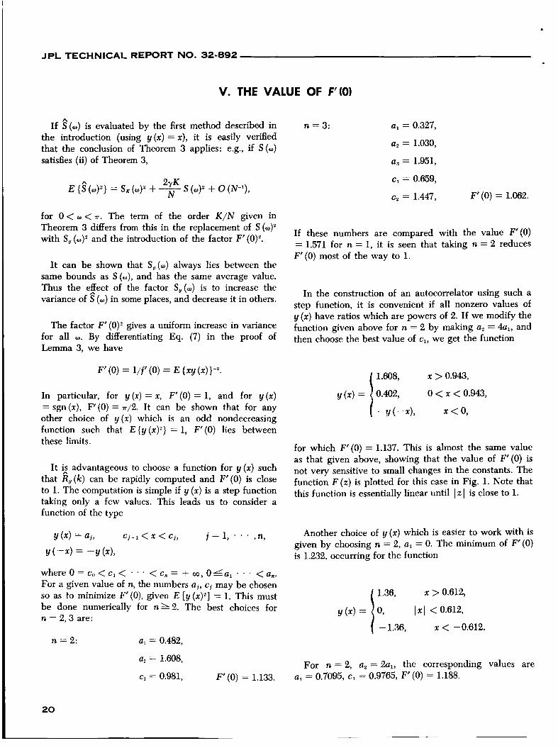
for which F ’ ( 0 ) = 1.137. This is almost the same value as that given above, showing that the value of F ’ ( 0 ) is not very sensitive to small changes in the constants. The function F ( z ) is plotted for this case in Fig. 1. Note that this function is essentially linear until I z I is close to 1.

It $ advantageous to choose a function for Y (X) such computed and F’ (0) is close

is simple if Y (x) is a step function that R~ (k) can be to The taking only a few values. This leads us to consider a function of the type

Another choice of y(x) which is easier to work with is given by choosing n = 2, al = 0. The minimum of F’ (0) is 1.232, occurring for the function

Y (x) = ai, Cj-1 < x < Cj, i = 1 , . . . 9 n,

Y ( - X ) = - Y ( 4 , whereO=c , ,<c ,< . . . < c , = + o o , O I a , . . . <a,. For a given value of n, the numbers aj, c, may be chosen so as to minimize F’(O) , given E [y(x)’] = 1. This must be done numerically for n s 2 . The best choices for n = 2 ,3 are:

1.36, x > 0.612,

y(x) = 0, 1x1 < 0.612,

x < -0.612. I - 1.36, n = 2: al = 0.482,

a2 = 1.608, For n = 2, a’ = 2al, the corresponding values are

c1 = 0.981, F ’ ( 0 ) = 1.133. a, = 0.7095, c1 = 0.9765, F ’ ( 0 ) = 1.188.

20

JPL TECHNICAL REPORT NO. 32-892 a

f

I

I-

Fig. 1. The function F (z) when y (XI takes four values with a ratio of 1:4

REFERENCES

1. Goldstein, R. M., Radar Exploration of Venus, Technical Report No. 32-280, Jet Propulsion laboratory, California lnstitude of Technology, Pasadena, California, May 25, 1962.

2. Zygmund, A., lrigonometrical Series, 2nd edition, Chelsea Publishing Co., New York, N. Y., 1952, p. 136.

3. Courant, R., Differential and Integral Calculus, Vol. 1, lnterscience Publishers Inc., New York, N. Y., 1949, p. 256.

2 1

Documents

The Variance of Spectral Estimates - NASA · Technical Report No. 32-892 The Variance of Spectral Estimates Eugene R. Rodemich Richard M. Goldstein, Manager Communications Systems