1

TECHNICAL ANALYSIS WITH UNCERTAIN PREDICTIVE POWER:

THE EFFECTS ON PORTFOLIO CHOICE

TYLER TSZWANG KWONG*

Latest revision: 12th November, 2015

Abstract. Deviating from a conventional statistical testing approach, we analyze the economic relevance of technical analysis. Specifically, we assess how uncertainty in predictive power of technical analysis affects investors’ portfolio choice. Calibrating our model with CRSP stock index data, we find that, accounting for such uncertainty, investors allocate substantially less to stocks and time the market less aggressively. These effects are stronger under longer investment horizons. Furthermore, the utility loss of ignoring this uncertainty is sizable and increases with horizon at an increasing rate. JEL Code: G11 Keywords: portfolio choice, technical analysis, estimation risk

* School of Banking and Finance, The University of New South Wales, Australia; Email: t.w.kwong@unsw.edu.au

2

Technical Analysis with Uncertain Predictive Power:

The Effects on Portfolio Choice

1 Introduction

When an investor receives a “buy” signal from a technical trading rule,

how much should he trust this signal and adjust his allocations to stocks? The

literature provides limited guidance in answering this question because it is

commonly assumed that investors use an all-or-nothing strategy, namely they

allocate 100% of wealth to stocks whenever a buy signal is observed but

nothing otherwise. This assumption, however, is unrealistic because it

overlooks at least two important issues.

First, investors do not necessarily have strong faith in technical analysis.

After all, empirical findings of its usefulness are mixed and inconclusive. Early

studies, for example, Fama and Blume (1966) and Jensen and Benington

(1970), question the profitability of technical analysis in stock markets.

Although later studies increasingly provide evidence defending the usefulness

of technical analysis, for example, Brock, Lakonishok, and LeBaron (1992)1

and Lo, Mamaysky, and Wang (2000)2, there is still counter evidence such as

the works by Allen and Karjalainen (1999), Ready (2002), and Bajgrowicz and

Scaillet (2012).

Second and more importantly, investors’ allocations to stocks should be

optimally chosen in a utility maximization framework: an investor’s optimal

allocation may depend on, for example, his degree of risk aversion, wealth

level, prior belief and current assessment of the predictive power of the trading

1 Sullivan, Timmermann, and White (1999) show that their results are robust even after adjustment is made for data-snooping. However, the results are weakened in out-of-sample testing. 2 More recent studies include Han, Yang, and Zhou (2013) and Neely et al. (2014).

3

rule. When stock returns are possibly predictable, the optimal strategy may also

depend on the investment horizon.

Failing to account for these two issues, the ad hoc all-or-nothing

assumption is unlikely to represent a sensible use of technical analysis in real

world. In this paper, we study portfolio choice with technical analysis in a

utility maximization framework, with an emphasis on how uncertainty in

predictive power of technical analysis affects portfolio choice. We consider an

investor who uses a linear prediction model to forecast stock returns with a

binary “technical signal” (buy or sell) as the predictive variable. In this context,

uncertainty in predictive power is equivalent to an unknown slope parameter.

We assume that the investor follows a simple Bayesian approach to use the

sample evidence to update prior beliefs about the model parameters 3 and

incorporates the precision of the estimators into his expected utility. He then

chooses how to allocate his wealth optimally, between a risk-free asset and a

risky stock, by maximizing expected utility. This optimization problem is

typically called “portfolio choice with parameter uncertainty”. Also, the

uncertainty in model parameters is commonly called “estimation risk”.

We focus on the moving average crossover rule 4 as an example of

technical analysis. This rule uses two moving averages5 to generate technical

signals: a “buy” signal is generated when the shorter average is above the longer

average and a “sell” signal vice versa. The principle of this rule is to follow a

market and detect if a new upward trend has begun or that an old trend has

ended or reversed.

Our perspective differs from most previous studies in that we view

technical analysis as a source of information that is potentially useful to forecast

3 We also assume that the intercept parameter is unknown. 4 The moving average crossover rule is one of the most widely used technical trading rules by practitioners and is commonly studied in the literature. 5 For discretely observed data, an -periodn moving average is an average of the previous n

data.

4

returns and there is no reason why investors have to commit to any trading rule.

Our approach offers a number of useful insights about technical analysis. First,

instead of testing whether the slope parameter is statistically significant, we can

incorporate the prediction model in a portfolio choice problem to study

economic relevance of technical analysis—how much would a utility

maximizing investor trust a “buy” signal and adjust his allocations to stocks?

Second, we derive an approximated solution for the optimal allocation to stocks,

which is explicit up to the investors’ moment estimates and investment horizon.

Third, we show quantitatively how the uncertainty in predictive power of

technical analysis affects market timing, while such uncertainty concern is

omitted from most previous studies. Fourth, we show that investors with shorter

investment horizons do not bear much utility loss even if they ignore such

uncertainty. By contrast, such utility loss is sizable for investors with longer

horizons. This implication helps to explain why short-term speculators seem to

favor technical trading even though the usefulness of technical analysis is often

questioned.

Although, to the best of our knowledge, there is no direct study

addressing our topic, we do get some useful insights from the current state of

literature. The effect of uncertain stock return predictability on portfolio choice

is studied by, for example, Stambaugh (1999), Barberis (2000), and Xia (2001).

They show that when a predictive variable has uncertain predictive power, a

sensible investor would choose his portfolio allocation according to his current

assessment of the conditional mean and the variance of his estimate for the

slope parameter. Further, the portfolio allocation may be sensitive to the

investment horizon. The authors also show that, in general, ignoring estimation

risk results in a substantial opportunity cost to the investor. We, however,

consider technical signals rather than the dividend yield which is commonly

studied in the literature. We shall show that it is slightly more complicated to

5

account for estimation risk when the predictive variable is a technical signal.

The reason is that the law of motion of the technical signal (as a function of past

stock prices) is determined by the prediction model itself but not an external

model. Therefore, the same source of estimation risk, namely having unknown

parameters in the prediction model, concurrently affects the forecasts of stock

returns and technical signals. We use a relatively simple, but otherwise

standard, Bayesian approach to account for estimation risk—selecting the most

appropriate econometric approach is beyond the scope of this paper.6 Zhu and

Zhou (2009) develop a model to justify why technical analysis, specifically the

moving average trading rule, can improve an investor’s opportunity set. Instead

of constructing unconditional forecasts of stock returns, we assume the investor

continuously infers information from technical signals to make conditional

forecasts7. Based on a similar conceptual framework to that of Zhu and Zhou

(2009), Zhou, Zhu, and Qiang (2012) test their one-period moving average

strategies and conclude that the proposed strategies outperform other strategies

that completely disregard the usefulness of moving averages. We instead

consider a long-horizon investor and study the effects of estimation risk on

portfolio choice and investor welfare, which are understudied in the context of

technical analysis.

Beyond academic studies, technical analysis has been widely used by

sophisticated practitioners and is considered an important tool for stock

investment. Menkhoff (2010) carries out a survey of fund managers 8 in

2003/2004. The respondents are 692 fund managers in five countries: United

6 There are alternative approaches to address estimation risk, for example, out-of-sample testing, correction factors, and randomization methods such as bootstrapping and Monte Carlo simulation. 7 We use “conditional forecast” to mean any approach that goes beyond using a single overall average, or unconditional mean, for forecasting. 8 The author justifies his sample choice by two reasons: first, fund managers have evolved as the most important group in modern financial markets; second, fund managers are highly qualified market participants compared to typical individual investors.

6

States, Switzerland, Germany, Italy, and Thailand and the majority of the

surveyed fund managers specialize in stock markets. The survey indicates that

87% of respondents use technical analysis and a major group (18%) prefers

technical analysis to other tools for investment decisions, including learning

fundamental information from the market. This survey shows that a substantial

proportion of technical analysis users has high reasoning power. Therefore, it is

relevant to consider a more realistic use of technical analysis through a portfolio

choice model and examine its economic relevance by studying the model

implications.

The paper is organized as follows. The next section discusses some issues

about technical analysis and portfolio choice with a prediction model. Section II

introduces our model. Section III describes the data and calibrates the model.

Section IV studies the model implications. Section V summarizes and concludes

the paper.

2 Background

There are four issues about technical analysis that are worth clarifying.

First, if stock returns are predictable9, then some technical signals may have

predictive power; if stock returns are independent and identically distributed,

then no technical signal can have predictive power. By analogy, no accounting

information or macro variable can have predictive power either. At minimal,

technical analysis summarizes some time-series properties of stock prices,

although their statistical properties are not well studied.

Second, technical analysis is a study of market price adjustments. The

equilibrium price adjusts to new information every day. The adjustment reflects

shifts in demand and supply as a result of the reactions of all market participants

9 For example, Bossaerts and Hillon (1999) provide strong evidence for in-sample return predictability using an international stock market dataset, although they fail to demonstrate out-of-sample predictability. However, Cochrane (2008) points out that poor out-of-sample performance is not a test against predictability.

7

to new information. However, this adjustment can be sluggish due to various

reasons such as noise, market frictions, and investors’ herding behavior. Noisy

rational expectations models and feedback models, among others, attempt to

provide theoretical justification for sluggish price adjustments. For example, see

Working (1958), Brown and Jennings (1989), and Wang (1993) for noisy

rational expectations models; De Long et al. (1990) and Shleifer and Summers

(1990) for feedback models. The common implication of these models is that

systematic adjustments in stock prices induce short-term serial correlations.

That is, the current price need not fully reveal all available information.

Therefore, technical signals may indicate the likely direction of price

adjustment.

Third, showing predictive power of a trading rule does not itself rebut

market efficiency10. Forecast errors can be large regardless of the quality of

parameter estimation. Therefore, the investor’s portfolio need not generate any

significant abnormal return after adjustment for risk and transaction costs.

However, an investor may disadvantage himself if he completely ignores

technical signals. For example, Han, Yang, and Zhou (2013) show that some

technical signals contain unique economic information that is not already

contained in other information sources.

Fourth, investors may well recognize that technical signals need not be

the most powerful class of predictive variables11 for stock returns, but other

variables are typically not observed frequent enough for real-time trading. In

particular, technical signals can be valuable to investors who engage in high

frequency trading, for example, investment banks, pension funds, mutual funds,

and other buy-side institutional traders.

10 Fama (1970) emphasizes that the notion of market efficiency does not necessarily imply successive price changes to be statistically independent. 11 There are many well-studied predictive variables for stock returns, for example, dividend yields, earnings-price ratio, term spreads, and expected inflation.

8

There are two features about portfolio choice with a prediction model that

are worth emphasizing. First, the true values of the model parameters are not

necessarily relevant to an investor with a finite horizon. To be precise, consider

the following linear prediction model for stock returns: Rt+1 = β0 + β1Xt + εt ,

where Xt is a binary technical signal12. Given a sample of T observations on

Rt+1 and Xt , let 0 1,ˆ )ˆ( T Tβ β denote some estimators of 0 1( , ).β β The true values of

the model parameters are often justified by the probability limit given by

(β0 ,β1) = plim T →∞(β0T , β1

T ). However, the finite sample estimates 0 1,ˆ )ˆ( T Tβ β are

the parameter values directly relevant for constructing forecasts, even though

their values need not be close to the hypothetical true values.

Second, a sensible investor who uses technical signals for forecasting

stock returns would take into account estimation risk when determining the

optimal allocation. Indeed, even if the estimators have good statistical

properties, the sample evidence need not fully reflect the future predictive

power because of the random variation of sampling. Under the Bayesian

approach, the investor integrates his expected utility over the unknown

parameter space for portfolio optimization. The resulted optimal portfolio

strategy incorporates the degree of uncertainty about the unknown parameters,

often measured by the covariances of the estimators 0 1ˆ ˆ, )( .T Tβ β Studies sharing

this idea include Bawa, Brown, and Klein (1979), Kandel and Stambugh (1996),

Brennan (1998), Barberis (2000), Jacquier, Kane, and Marcus (2005), and Xia

(2001).

12 For example, a “buy” signal is represented by 1tX = and Xt = 0 for a “sell” signal.

9

3 The Model

3.1 The Basic Setting

Consider an investor with a long horizon who trades continuously in a

two-asset economy in which a risk-free asset pays an instantaneous rate of

interest r, and a risky stock represents the aggregate equity market.

We fix a finite horizon [0, ].T The cum-dividend stock price grows

according to the following process:

*dd d ,t

t tt

Pt B

Pµ σ= +

where the percentage volatility σ is a known parameter; Bt* is a Brownian

motion defined on the probability space * *),( ,Ω P F with a standard filtration

* * : .t t T= ≤F F However, the instantaneous percentage drift, µt , is unknown to

the investor.

The investor observes a technical signal ,tX a function of past stock

prices, that is potentially useful to estimate ,tµ or equivalently, to forecast

d / .t tP P Let S and ,L with 0 ,S L T< < < be two lookback periods. We define

X t =1 if Dt

S ,L > 0,

0 otherwise,

where

, 1 1d d

t t

t S t

S Lt

L

P PDS L

τ ττ τ− −

≡ −∫ ∫

is the difference of two moving averages of stock prices. We assume the history

Pt : −L ≤ t ≤ 0 is known. It is also useful to note that the dynamics of ,S L

tD are

given by

, 1 1( ) ( )d d .S L

t t t S t t LP P

LD t

SP P− −

−

= − −

10

Let P denote the investor’s subjective probability measure, and

: ,t P tτ τ= ≤F with *,t t⊂F F denote the investor’s information set at time t.

Under the reference model probability ,P the investor conjectures a linear

predictor β0 + β1Xt of µt , and thus the cum-dividend stock price is represented

by the following “linear prediction model”:

d Pt

Pt

= (β0 + β1Xt )d t +σ d Bt ,

where 0 1( , )β β are unknown model parameters; tB is a standard -BrownianP

motion adapted to the investor’s information set .tF While the same linear

prediction model is also used in Xia (2001), there are two structural differences

for our predictive variable: first, the technical signal t

X is a binary variable;

second, it is a function of past stock prices only with no assumption on its law

of motion required. The common assumption that the predictive variable

follows a (univariate) Markovian mean-reverting process is therefore not

applicable. Here, we also relax the assumption that the intercept parameter is

known.

For any fixed point of time t in [0,T ), given an initial wealth Wt and the

investment horizon T , the investor chooses a portfolio allocation ξ to

maximize his expected utility of wealth,

max E[ |( ],)T tU Wξ

F

given the wealth dynamics

dWτ

Wτ

= r dτ + ξ(β0 + β1Xτ − r)dτ + ξσ d Bτ .

We use the notation τ above because the letter t is already used to denote the

fixed chosen point t. Note that ξ is a constant to solve for each point of time .t

11

We call the sequence of solutions to ξ a “rolling strategy” because it is

essentially a “buy-and-hold strategy” with continuous rebalancing.13 Since the

conditional distribution of WT varies over time due to continuously updated

information, so does the maximizer

* argmax E[ ( ) | ].t T tU W

ξ

ξ ≡ F

We call *tξ the “optimal allocation”14 conditional on current information. Our

behavioral assumption that the investor follows this rolling strategy may be

strong. A more realistic model would allow for a dynamic strategy to account

for the possibility of learning the model parameters in the future, as in Brennan

(1998) and Xia (2001). However, we believe that this “rolling” assumption can

also give us useful implications for portfolio choice and investor welfare

because it allows us to obtain a traceable solution for optimal stock allocations.

In this paper, we assume the power-utility function

1

( ) , 1,1

TT

WU W

γ

γγ

−

>−

=

where γ is the investor’s risk-aversion parameter. We shall only consider

investors with a risk-aversion parameter greater than the logarithmic case.

3.2 The Investor’s Optimization Problem

It is useful to rewrite the utility function as

U (WT ) =

exp[(1−γ ) logWT ]

1−γ

and apply Ito’s rule to obtain log ,TW

13 The buy-and-hold strategy is considered by, for example, Stambaugh (1999), Barberis (2000), and Avramov (2002). 14 The solution is “optimal” subject to our model assumptions and specifications.

12

22

20 1( )

( ),

log log [ ]( )T t

T

Tt

t

W W r r

BB

T tσξ β β ξ

ξσ

= + + + − −

+ −

−X

where we define the variable

,1

d

T

Tt

t

XT t

τ τ≡− ∫X

which can be interpreted as the average value of the technical signals over the

period [ , ].t T Since 0 1, , )( Ttβ β X are not adapted to ,tF they are considered

random variables at time t.

Let 0 1T

t tθ β β≡ + X denote the “average percentage drift” over the

remaining investment horizon. By the law of total expectation, we have

) )E[ ( | ] E[ ( | ( )d, ] | ,T t T tt t t tU W U W θ φ θ θ=R

∫F F F (1)

where )( |t tφ θ F is the conditional density of tθ and the integral is taken over the

real line .ℝ By log-normality, the expectation inside the integral is

2

(1 )( )

2

E[ ( , ]) | )

exp (1 ) ( )( )

(

.

r T tT t t t

t T

U W e U W

tr

γ

γσ

θ

γ ξ θ ξ

− −=

− −× − −

F

Suppose that tθ follows a conditional Gaussian distribution with mean

E[ | ]t ttm θ≡ F and variance Var ],|[t t tv θ≡ F then equation (1) satisfies:

2

2

) |

exp (1 ) ( )

E[ ( ]

) [ (1 ( ,)] ( )

T t

t tm v T

U W

T t trξγ ξ γσ γ− − + − −∝ − −

F (2)

where the notation “ ∝ ” indicates that the expression holds as an equality

subject to a multiplicative term independent of ξ.

Even if θt is non-Gaussian, we can approximate it by a Gaussian process

that matches the first and the second moments. We take (2) as the true

expression and optimize it with respect to ξ to obtain the optimal allocation

13

*

2.

( ( )1)t

t

t

m r

T tvξ

γσ γ −−=

+ − (3)

3.3 The Investor’s Inference Problem

Let us use the notation β ≡ (β0 ,β1). By the law of total expectation, we

can evaluate tm as follows,

0 1

0 1

E[ | ] E E [ | , ] |

E[ | ] E[ ( ) | ],

t t t t

t

Tt t

t t

mβθ β β β

β β β

≡ = +

= +

X

X

X

E

F F F

F F

where we define the function 2:t →XE R R by

( E[ , ]) | ,Tt t tβ β≡XE X F

which is a function of β to be found. The operator E β ⋅ indicates that the

expectation is taken over the distribution of β , and similarly, TtX for E [ ].⋅X In

the reference model ,P the random process : TX tτ τ< ≤ is determined by

: ,P t Tτ τ< ≤ which depends on ,β thus the expectation E[ | ],Tt t βX F also

depends on β and cannot be factored out from the outer expectation E .β ⋅ By

contrast, if the law of motion of tX were not determined by the prediction

model itself, we would simply have 0 1E[ | ] E[ | ] E[ | ],t t t t

T

tm β β ⋅= + XF F F which

would be linear in the conditional expectations of 0 1( ), .β β

Similarly, by the law of total variance, we can evaluate vt as follows,

0 1

0 1

21 10

Var Var

V

[ | ] E [ | ,

ar

) | V

] |

E [ | , ] |

E[ ( ] ar[ ( ) | ],

Ttt t tt

Tt

t tt

t

t t

t

v β

β

θ β β β

β β β

β β β β β

≡ = +

+ +

= + +

X

X

X X

X

X

V E

F F F

F F

F F

where we define the function 2:t+→X

V R R by

) Var[ | ,( ],Ttt tβ β≡X

V X F

which is a function of β to be found. The operator Var β ⋅ indicates that the

variance is taken over the distribution of β , and similarly, TtX for Var [ ].⋅X

14

Let E[ | ]t tmβ β≡ F and [V | ]t tv

β β≡ F denote the conditional mean and the

variance-covariance matrix of the investor’s estimate of β. We assume that the

investor has a bivariate Gaussian prior probability distribution over β , with

mean vector m0β and variance-covariance matrix v0

β . Following Liptser and

Shiryaev (2001), the distribution of β conditional on tF is also Gaussian with

mean vector mtβ and variance-covariance matrix vt

β .

Proposition 1. Given the prior probability distribution of β is Gaussian with

mean vector m0β and variance-covariance matrix v0

β , the solutions to mtβ and

vtβ are

1

0 002

0 0

2

d( )d ,

t t

t

v v Pm I X X Xm

P

β ββ β τ

τ τ ττ

τσ σ

−

= + +

⊤∫ ∫

1

002

0

( )d ,

t

t

vv I X X v

ββ β

τ τ τσ

−

= +

⊤∫

where (1, )t tX X=

⊤ is a 2 ×1 vector; I is a 2 × 2 identity matrix.

We use the following notation to denote the elements of mtβ and vt

β ,

mtβ =

mtβ0

mtβ1

, vt

β =vt

β0 vtβ0 ,β1

vtβ0 ,β1 vt

β1

.

Also, we use /[ ]i if f β≡∂ ∂ ∂ and 2, [ ] / ,i j i jff β β≡∂ ∂ ∂ ∂ , 0,1,i j = to denote

the partial derivatives of a given function .f

Proposition 2. Suppose that the functions tXE and t

XV are continuously

differentiable around ,t

mβ

then mt can be expressed as the following Taylor

series

15

0 1 1 0

1 1

1 0 1

01

,02

1 1,1

,0 0,1

12

[ ] ( [ ])

( [ ] [ ])

( [ ] [ ]) ,

t t t t t

t

t t

t t

t t

t

t t t

m m m m v

m v

m v H

β β β β

β β

β β β

= + +

+ +

+ + +

X X

X X

X X

E E

E E

E E

∂

∂ ∂

∂ ∂

(4)

and vt can be expressed as the following Taylor series

1 1 1 0

1 1

1 1

1 1

1 1 0 1

2 2 20,0 0

21 1,1

21

20 0,1

,0

12

1

12

[[( ) ] ( ) [ ] (1 )

2 [ ] ( ) [ ]

( )

2 [ ]

2(1 )( ) ,

]

[ ]

[ ] ( )

[ ] [ ]

t t t

t t t

t t

t t

t t

t t t t t

t t

t t

t

t t tt

t

t

v m m m v

m m

m v

m m

m m v O

β β β β

β β

β β

β β

β β β β

= + + +

+ + +

+ +

+

+ + + +

+

X X X

X X X

X X

X X

X X X

V V E

V V V

E E

V V

E E E

∂ ∂

∂ ∂

∂

∂ ∂

∂ ∂

(5)

where ,tXE ,t

XV and their partial derivatives are evaluated at mt

β; Ht and Ot

are remainder terms.

We give the proofs of these propositions in Appendix A.

To our knowledge, closed-form solutions for tXE and t

XV are not feasible.

Therefore, we develop estimators and use Monte Carlo simulation to estimate

these functions. Given any arbitrary positive integer n, we define the quantities

/ ,t T n∆ ≡ / ,nL T≡ℓ and / ,s nS T≡ where “ ” is the floor function. For a

sufficiently large n, we have L t∆≃ ℓ and .S s t∆≃ The notation “ ” means

“approximately equal to or equal to”. We partition the time interval [ , ]t T− ∆ℓ

into n+ℓ equidistant subintervals,

00 ,s nL t tt TS t− −− < < << − < = < =ℓ ⋯ ≃ ⋯ ⋯≃

and approximate any t in [ , ]L T− by jt if 1 ,jjt t t− < ≤ , , .nj = − …ℓ Next, we

consider the following Euler approximation scheme:

1 0 1ˆ ˆ ( )ˆ ˆ ,j j j j jt t t t tP P P X t tβ β σ+ + ∆ + ∆ = + ε (6)

1

, , 1ˆ ˆ ˆ ˆ ˆ1( ) ( )ˆ ,j j s j jj j

S L S Lt t t tt tD

sD P P P P− −+

= + − − − ℓℓ (7)

16

11

,ˆif ˆotherwis

,

0 e,

1 0j

j

S L

tt

DX +

+

>=

(8)

with Pt j

= Pt− j∆t if ,j i≤ , 10, ;i n −= … jtε are independent standard Gaussian

random variables.

To simulate a trajectory of Xt j

: j = i,…,n −1, , 10, ,i n −= … we start

from the initial values ( ,ˆ ˆ )i it t t tP XP X= = and proceed recursively according to

the Euler scheme (6)-(8). We then calculate the sum

1

1 ˆˆj

n

tTt

j i

X tT t

−

=−

≡ ∆∑X

to approximate the stochastic integral .TtX Let ,

ˆ Tt kX denote the sum calculated

using the k -th trajectory, , .1,k K= … To estimate the moment ,( )t βXE we use

the estimator

1

,ˆˆ ( )

1; ,T

t t k

K

k

tK

β=

≡ ∑XεE X

and similarly,

2

1

,2

1

,ˆ ˆˆ 1 1

; (( )) T Tt t k

K

k k

t

K

ktK K

β= =

−

≡

∑ ∑

XXεV X

for the moment ( ),t βXV where 1 1

,1 ,( , , )j j

n nt t j i t K j i

− −= == …

ε ε ε is an (n − i) × K matrix

of independent standard Gaussian random numbers. We use the argument ( ); t⋅ε

to emphasize that the values of tXE and t

XV depend on .t

ε By fixing t

ε for each

,t the estimators tXE and t

XV are smooth in β. Thus, we can evaluate the partial

derivatives in the Taylor series of mt and vt , given by (4)-(5), using finite

difference approximation. We present the required formulas in Appendix B.

17

4 Data, Model Calibration, and Some Empirical Facts

We measure the horizon T in years and consider daily intervals (with

step size 1252 )t∆ = small enough for good discrete approximations to the

continuous-time processes in the model. We use the inflation adjusted CRSP

index (including distributions) on a value-weighted basket of stocks listed in

NYSE, AMEX, and NASDAQ as an example of the risky stock. We obtain the

nominal daily index data for the period 2nd January 1980 to 31st December 2014

from the CRSP VWRETD file under the folder named “Index/Stock File

Indexes”. Then, we make a month-by-month inflation adjustment by dividing

the stock index series by the consumer price index (CPI), using January 1980 as

the base month. The CPI data are obtained from the CRSP inflation file under

the folder named “US Treasury and Inflation Indexes”. The standard deviation

of the daily inflation adjusted index returns is 1.083%. Dividing this figure by

t∆ gives σ = 0.172. We also obtain the nominal monthly interest rate data

from the CRSP 30-day Treasury bill file. The monthly average interest rate is

0.382%, and 0.267% for the monthly average of the rate of change in CPI.

Thus, the implied daily real interest rate is 0.004%. Dividing this figure by t∆

gives r = 0.01. For the Euler approximation scheme, we use 2000K =

trajectories, although we find that even 500K = would give similar results.

As an example, we use the moving average crossover rule with 1-day and

100-day moving averages. In terms of the model notation, we have s = 1 and

100.=ℓ To obtain reasonable priors 0 0( , ),m vβ β we use the inflation adjusted

index data for the subsample period 2nd January 1980 to 22nd December 1994

(leaving 20 252× days for the out-of-sample period) to run the regression:

1

0 1( ) ,j j

j j

j

t tt t

t

PPtX

Pβ β ε+ −

= + ∆ +

18

where 1jtX = if the 1-day moving average is above the 100-day moving

average at time ,jt and zero otherwise. We then take the ordinary least squares

estimates as the priors:

m0β =

0.058

0.061

, v0

β =0.004 −0.004

−0.004 0.006

.

Figure 1 plots the time series of the intercept and the slope estimates

when the investor starts investing on 23rd December 1994 with the prior

Gaussian distribution with mean vector and variance-covariance matrix

0 0( , ).m v

β β These time series end on the last trading day of year 2014. Observe

that the slope estimates roughly follow a downward trend over the horizon but

clearly stay above zero. The estimates of the intercept loosely form a mirror

image of that of the slope estimates. Although the intercept estimates are larger

than the slope estimates in general, it is evident that the slope estimates have a

clear impact on the conditional forecasts of stock returns. In summary, the data

may encourage some investors to believe that the technical signals possibly

have predictive power on stock returns (even if the true but unknown value of

1β is zero).

5 Analysis and Results

5.1 Mean and Variance Decompositions

We express the expected value and the variance of the average percentage

drift, ( ),,t tm v as the following linear forms:

0 1 0 11 010 , ,t t t t t t t t tm v v v Hmβ β β βπ π π= + + + +ɶ (9)

0 1 0 10 1 01 , .t t t t t t t ttv v v v Ovβ β β βλ λ λ= + + + +ɶ (10)

The remainders Ht and Ot correspond to the ones in Proposition 2, and the

definitions of the coefficients follow accordingly: 0 1 ,t t t tmm mβ β≡ +ɶ

XE

1 2( ) ,t t tmvβ≡ɶ XV and so on. We call ,( )

t tm vɶ ɶ the “basic component” of ( ).,

t tm v We

19

also call ,( )t t

m vɶ ɶ the “estimation-risk ignorant estimates” because they disregard

any estimation risk adjustment. For simplicity, we approximate mt and vt by

summing only the first four terms, although one could improve the

approximation by including higher-order moments and derivatives.

We divide equation (9) by mt to obtain

0 1 0 11 01 ,0

0 1 01

,

1 ,

t t t t t t t t

t t t t t

t t t t

m v v vm m m m m

M M

m

MM

β β β βπ π π= + + +

= + + +

ɶ

ɶ

where t

Mɶ is the percentage composition of the basic component ;t

mɶ

0 1 01, and , ,t t t

M M M for the estimation-risk adjustment components. Similarly, we

divide equation (10) by vt to obtain

0 1 0 10 1 01 ,

0 1 01

,

1 ,

t t t t t t t t

t t t t t

t t t t

v v v vv v v v v

V V

v

VV

β β β βλ λ λ= + + +

= + + +

ɶ

ɶ

where t

Vɶ is the percentage composition of the basic component ;t

vɶ

0 1 01, and , ,t t t

V V V for the estimation risk adjustment components.

We consider four investment horizons, 5,10,15,20.T = For each horizon,

we perform the mean and the variance decompositions at five points of time,

,t Tδ= 3 2511 14 2 4 2520, , , , .δ = Panel A of Table I displays the results of the mean

decomposition. We observe that the basic component accounts for roughly

100% of tm most of the time while the estimation risk adjustment components

are relatively small. Our results suggest that ignoring estimation risk does not

materially bias the expected value of average percentage drift .t

θ

Panel B of Table I displays the results of the variance decomposition. We

observe that the size of the estimation-risk ignorant component is materially

smaller than that of the estimation risk adjustment components. Notably, the

estimation-risk ignorant component becomes essentially 0% towards the end of

20

the horizon. Our results suggest that ignoring estimation risk materially

underestimates the variance of the average percentage drift.

Note that both ( , )t t

m v and ( , )t t

m vɶ ɶ depend on the technical trading rule and

the stock price data. Therefore, their relative sizes can only be determined

empirically. Without actual data, we would have an inconclusive theoretical

discussion.

5.2 Horizon Effect and Hedging Demand

Let us define the “suboptimal allocation” by

2

.( (1) )

tt

t

r

T t

m

vξ

γσ γ −−≡

+ −

ɶɶ

ɶ (11)

This is the allocation that would be made if the investor used the estimation-risk

ignorant estimates, ).( ,t t

m vɶɶ Equivalently, we obtain t

ξɶ by setting 0 0 11 ,( , , )t t t

v v vβ β ββ

to zero in the optimal allocation *

tξ given by (3). Both the optimal and the

suboptimal allocations depend on the remaining investment horizon, :T t−

directly through the denominators; and indirectly through the mean and the

variance of average percentage drift ( , , , ).t t t t

m v vm ɶɶ The influence of the

remaining horizon on the portfolio allocation is commonly called the “horizon

effect”. Also, we call the difference of the two allocations, * ,t t t

ξ ξ−∆ ≡ ɶ the

investor’s “hedging demand”. We can interpret this quantity as an allocation to

hedge against estimation risk.

We consider three values of the risk-aversion parameter, 5,7,9.γ = For

each investment horizon, 5,10,15,20,T = we calculate the optimal allocation,

the suboptimal allocation, and the hedging demand at five points of time,

,t Tδ= 3 2511 14 2 4 2520, , , , .δ = Table II displays our results. Consider time 0.t =

Observe first that, for all values of ,γ the optimal allocation monotonically

decreases as the horizon increases while the suboptimal allocation is not

21

sensitive to the horizon. This is because the empirical values of t

vɶ are

sufficiently small that the adjustment term ( )t

v T t−ɶ in (11) does not have a

strong effect on the suboptimal allocations. Second, the optimal allocation

decreases more sharply for higher value of γ as the horizon increases. Overall,

the hedging demand is increasing in horizon but decreasing in risk-aversion

parameter.

Next, we look at other points of time along the investment horizon. Our

results show that the horizon effect is clear. At time 34 ,t T= with only a quarter

of horizon remaining, the values of the hedging demand are still above 2%.

However, the hedging demand declines with the remaining horizon. The reason

is that as the estimates become more precise and the remaining horizon

decreases, the compounding effect of estimation risk becomes less severe.

The notion that investors bearing estimation risk may allocate less to

stocks for longer horizon is not new. For example, in the context of an IID

model for returns, Brennan (1998) finds that the dynamic allocation declines

monotonically as the horizon is reduced when the investor is more risk tolerant

than a logarithmic investor; in the context of a predictive VAR model for

returns, Barberis (2000) finds that the allocation can decrease with horizon

when the investor uses a buy-and-hold strategy. Stambaugh (1999) and Xia

(2001) also show that the allocation can decline eventually when the horizon

becomes sufficiently long, although the allocation can first increase with

horizon. Our results are consistent with these findings.

However, in these studies, the portfolio allocation equation is not

characterized in a form that signifies the role of remaining horizon, .T t−

Jacquier, Kane, and Marcus (2005) derive a closed-form solution for a buy-and-

hold strategy that incorporates estimation risk in the context of an IID model for

returns. Their findings on horizon effect are qualitatively consistent to that of

Brennan (1998). Similarly, we make the role of remaining horizon more

22

tractable in the context of a prediction model. Because our conclusion on

horizon effect depends on our model assumptions, model specifications, data,

and estimation strategy, it is not a direct consequence of known results.

5.3 Market Timing Effect

When stock returns are possibly predictable, the portfolio allocation can

depend on the current value of the predictive variable. This is called the “market

timing effect”. For our model, when the estimate of the slope parameter is

positive, then a buy signal implies a higher expected stock return. This attracts

the investor to increase his allocation in the risky stock. However, since the

portfolio allocation also depends on other state variables, not just the technical

signal, it is difficult to study the market timing effect conditional on all other

state variables. As a compromise, for any given portfolio allocation strategy ,ξ

we calculate the averages of | 1t t

Xξ = and | 0t t

Xξ = in a fixed time interval

and interpret their difference as the unconditional average market timing effect.

We again consider the optimal and the suboptimal strategies for four

investment horizons, 5,10,15,20,T = and three values of risk-aversion

parameters, 5,7,9.γ = We compute the averages using the subsample period

from 23rd December 1994 to 20th December 1999 ( 5 252× trading days)

because it is the widest time interval in which our portfolios are built using the

same data. During this subsample period, we observe a reasonable mix of buy

and sell signals. Our analysis tries to study how the market timing effect varies

with horizons.

We display the results in Table III. Firstly, observe that the average

market timing effect is positive and it has a range of 1% to 5.5% (per trading

day). While we consider this effect economically significant, it is far from 100%

for all portfolios considered in this paper. In this regard, it is hard to justify the

use of all-or-nothing strategy commonly assumed in the literature. Secondly, we

23

observe two patterns of average market timing effect: it decreases as investment

horizon increases; and it also decreases as the risk-aversion parameter increases.

Thirdly, we note that the average market timing effect associated with the

optimal strategy decreases more notably with horizon compared to that of the

suboptimal strategy. We highlight the differences in average market timing

effect between the optimal and the suboptimal strategies in Figure 2. We see

that, except for the shortest horizon considered ( 5),T = the average market

timing effect is stronger for the suboptimal strategy. We also see that the

differences are more notable as the horizon increases and the risk-aversion

parameter decreases. Overall, our results show that market timing strongly

depends on risk aversion, investment horizon, and attitude towards estimation

risk.

Our findings relate to that of Zhu and Zhou (2009) in the following sense.

Although our models differ in how the investor infers information from the

technical signals, we show that it is optimal for the investor to allocate an

additional proportional of his wealth to the stock when he observes a buy signal.

Our model, however, allows the investor to continuously assess the predictive

power of the signals based on sample evidence and he adjusts his portfolio

allocation accordingly. In particular, while the estimates of the slope parameter

remain positive in our sample period, it is possible to become negative. In that

case, the investor would actually decrease his allocation to the risky stock even

though a “buy” signal is observed. This is possible because if the current price

is well above the moving averages, the chance of a price reversal is also high.

Therefore, the sign of the slope estimate depends on whether the data suggest

that the buy signals are more often related to new upward trends or price

reversals on average. When the statistical relationships are mixed, the slope

estimate can be close to zero and the signals become uninformative. Our idea

differs from the conventional assumption that the investor necessarily increases

24

his allocation (and by the same proportion of wealth) whenever he observes a

buy signal.

5.4 Welfare Costs of Ignoring Estimation Risk

Given an allocation t

ξ to the risky stock, we define a function J by

2

2

( , , , ; )

( )exp ( ) [ (1 ( )1 ) ( ) (] ) .t

t t t t

t t t tm v T t

J t W m v

U W r T tξ

ξ

γ ξ γσ γ≡ − − − −−− +

This is the investor’s maximized expected utility at time .t Next, we define the

“welfare cost” of using the suboptimal allocation t

ξɶ by the quantity t

∇ that

satisfies the equality

*( ,1, , ; ) ( ,1 , , ; ).t t t t t t t

J t m v J t m vξ ξ= + ∇ ɶ

The welfare cost t

∇ measures the percentage wealth compensation

required to leave the investor, who has $1 today to invest up to the horizon,

indifferent between the optimal and the suboptimal allocation strategies. Similar

measures are used in the literature, for example, Campbell and Viceira (1999),

Xia (2001), and Han, Yang, and Zhou (2013). By construction, the value of J is

maximized at all time t if t

ξ is the optimal allocation *.t

ξ Hence, the welfare

cost t

∇ is always non-negative. We are interested to see the size of this value to

study how costly is it to an investor if he ignores estimation risk.

We again consider four investment horizons, 5,10,15,20,T = and three

values of risk-aversion parameters, 5,7,9.γ = For each horizon, we compute

the welfare cost at five points of time, ,t Tδ= 3 2511 14 2 4 2520, , , , .δ = Table IV

displays the results. We see two patterns of welfare cost. First, it increases

substantially as the horizon increases. For the shortest horizon considered

( 5),T = at time 0,t = its range is 0.352% to 0.530%. By contrast, for the longer

horizons, 15,20,T = the range is 6.394% to 21.474%, and the welfare cost

remains above 3% for at least one quarter of the horizon. Our results imply that

25

it can be costly to ignore estimation risk for investors with a longer horizon.

This is because the suboptimal strategy results in more severe overinvestment

for longer horizons. Relatively speaking, estimation risk may be less of a

concern for investors with shorter horizons. To further signify the magnitude of

welfare cost, we fix the time at 0t = and plot it as a function of horizon and

risk-aversion parameter in Figure 3. The results show that the welfare cost

increases with horizon at an increasing rate. The second pattern we observe is

that the welfare cost increases as the risk-aversion parameter decreases and the

increase is stronger for longer horizons. For example, for 10,T = the welfare

cost increases from 2.245% to 3.434% as γ decreases from 9 to 5 at time 0t = ;

for 20,T = the welfare cost increases from 13.469% to 21.474%.

To summarize, using historical data on stock returns and technical

signals, we gain some insight about the opportunity cost to an investor if he

ignores the uncertain predictive power of the technical signals generated by the

moving average trading rule. Our results complement studies using other

predictive variables, prominently the dividend yield. Although the general

effects of neglecting estimation risk in portfolio choice are well studied, without

an actual application to technical analysis, it would be hard to speculate the

magnitude of these effects in real world.

6 Conclusion and Future Work

We have analyzed an investor’s portfolio choice problem in which he

forecasts stock returns using technical signals. We calibrate our model with

CRSP stock index data and find that if an investor considers the uncertainty in

predictive power of technical signals, he allocates substantially less of his

wealth to stocks and time the market less aggressively, the longer his

investment horizon. Moreover, we find that the opportunity cost of ignoring

such uncertain predictive power increases sizably with horizon at an increasing

26

rate. Our model implications contrast with the common assumption that

investors allocate 100% of wealth to stocks whenever they observe a buy signal

but nothing otherwise.

This study is only an initial attempt to incorporate information from

technical signals in a Bayesian portfolio choice problem. Although we have

considered the role of estimation risk, we have assumed that the investor

ignores the possibility of learning the model parameters in the future. An

important extension is to consider a dynamic portfolio strategy as in Brennan

(1998) and Xia (2001). Also, we have only considered the moving average

trading rule. Given our data and this particular trading rule, our results suggest

that ignoring estimation risk does not materially bias the expected average drift

of returns but materially underestimates its variance. As a consequence, the

optimal portfolio allocation is sensitive to the remaining horizon. Other more

elaborate rules, such as those depend on charting patterns considered by Lo,

Mamaysky, and Wang (2000), may give us a different insight. Our model can

be easily modified for these rules.

Appendix A. Proofs of Propositions

Proof of Proposition 1: This is a direct application of Theorem 12.7 in Liptser

and Shiryaev (2001, p. 36). Q.E.D.

Proof of Proposition 2: Equation (4) is the second-order Taylor series

expansion of 0 1

E[ | ] E[ ( ) | ]tt t t

m β β β= + XEF F around the point 0 1( , ).

t tm m

β β To

obtain equation (5), we find the second-order and the first-order Taylor series

expansions of the first and the second terms of

1 10

2 ) | VE[ ( ] ](ar[ ,) |t t tt t

v β β β β β= + +X XV EF F

respectively. Q.E.D.

27

Appendix B. Formulas for Finite Difference Approximation

We use the following partial derivative approximations:

0 01 1

0

, ) , ))

(,

2

(( t tt t

t

t

t

tm m m m

mβ ββ β

β δ δδ

+ −−≈

X X

X E EE∂

10 10

1

, ) , ))

2

(( ,

(t tt t t

t

t

t

m m m mm

β ββ ββ δ δ

δ+ −−

≈X X

X E EE∂

1 0 10 0 1

20,0

( ( ((

, ) 2 , ) , )) ,t tt t tt

tt

t t tm m m m m m

mβ β ββ β β

β δ δ

δ

− +≈

+ −X X X

X E E EE∂

1 0 10 0 1

21,1

( ( ((

, ) 2 , ) , )) ,t tt t t t

t

tt t

t

m m m m m mm

β β ββ β ββ δ δ

δ

− ++ −≈

X X X

X E E EE∂

0 0 0

0 0

1 1 1

1 1 0 1

0 1

20,1

2

2

( ( ((

(

, ) , ) , ))

2

, ) ( (

2

2 (

, ) , )

)

2

,.

t t t t t t

t

t t t t t t

t t

t t t

t

t t t

t

m m m m m mm

m m m m m m

m m

β β ββ β ββ

β β ββ β β

β β

δ δ δ δ

δ

δ δ δ δ

δ

δ

− −+ + +≈

+

− − − −−

+

+ −

X X X

X

X X X

X

E E EE

E E E

E

∂

Similar formulas are used for .t

XV We set 0.01.δ =

REFERENCES

Allen, F., & Karjalainen, R. (1999). Using genetic algorithms to find technical trading rules. Journal of Financial Economics, 51(2), 245-271.

Avramov, D. (2002). Stock return predictability and model uncertainty. Journal

of Financial Economics, 64(3), 423-458.

Bajgrowicz, P., & Scaillet, O. (2012). Technical trading revisited: False discoveries, persistence tests, and transaction costs. Journal of Financial

Economics, 106(3), 473-491.

Barberis, N. (2000). Investing for the long run when returns are predictable. Journal of Finance, 55(1), 225-264.

Bawa, V. S., Brown, S. J., & Klein, R. W. (1979). Estimation Risk and Optimal

Portfolio Choice (North-Holland, New York).

Bossaerts, P., & Hillion, P. (1999). Implementing statistical criteria to select return forecasting models: what do we learn?. Review of Financial Studies, 12(2), 405-428.

28

Brennan, M. J. (1998). The role of learning in dynamic portfolio decisions. European Finance Review, 1(3), 295-306.

Brock, W., Lakonishok, J., & LeBaron, B. (1992). Simple technical trading rules and the stochastic properties of stock returns. Journal of Finance, 47(5), 1731-1764.

Brown, D. P., & Jennings, R. H. (1989). On technical analysis. Review of

Financial Studies, 2(4), 527-551.

Campbell, J. Y., & Viceira, L. M. (1999). Consumption and portfolio decisions

when expected returns are time varying. Quarterly Journal of Economics, 114(2), 433-495.

Cochrane, J. H. (2008). The dog that did not bark: A defense of return predictability. Review of Financial Studies, 21(4), 1533-1575.

De Long, J. B., Shleifer, A., Summers, L. H., & Waldmann, R. J. (1990). Noise trader risk in financial markets. Journal of Political Economy, 98(4), 703-738.

Fama, E. F. (1970). Efficient capital markets: A review of theory and empirical work. Journal of Finance, 25(2), 383-417.

Fama, E. F., & Blume, M. E. (1966). Filter rules and stock-market trading. Journal of Business, 39(1), 226-241.

Han, Y., Yang, K., & Zhou, G. (2013). A new anomaly: The cross-sectional profitability of technical analysis. Journal of Financial and Quantitative

Analysis, 48(05), 1433-1461.

Jacquier, E., Kane, A., & Marcus, A. J. (2005). Optimal estimation of the risk premium for the long run and asset allocation: A case of compounded estimation risk. Journal of Financial Econometrics, 3(1), 37-55.

Jensen, M. C., & Benington, G. A. (1970). Random walks and technical theories: Some additional evidence. Journal of Finance, 25(2), 469-482.

Kandel, S., & Stambaugh, R. F. (1996). On the predictability of stock returns: An asset-allocation perspective. Journal of Finance, 51(2), 385-424.

Liptser, R., & Shiryaev, A. N. (2001). Statistics of Random Processes: II.

Applications (Springer-Verlag, New York).

Lo, A. W., Mamaysky, H., & Wang, J. (2000). Foundations of technical analysis: Computational algorithms, statistical inference, and empirical implementation. Journal of Finance, 55(4), 1705-1765.

Menkhoff, L. (2010). The use of technical analysis by fund managers: International evidence. Journal of Banking and Finance, 34(11), 2573-2586.

29

Neely, C. J., Rapach, D. E., Tu, J., & Zhou, G. (2014). Forecasting the equity risk premium: the role of technical indicators. Management Science, 60(7), 1772-1791.

Ready, M. J. (2002). Profits from technical trading rules. Financial

Management, 31(3), 43-61.

Shleifer, A., & Summers, L. H. (1990). The noise trader approach to finance. Journal of Economic Perspectives, 4(2), 19-33.

Stambaugh, R. F. (1999). Predictive regressions. Journal of Financial

Economics, 54(3), 375-421.

Sullivan, R., Timmermann, A., & White, H. (1999). Data-snooping, technical trading rule performance, and the bootstrap. Journal of Finance, 54(5), 1647-1691.

Wang, J. (1993). A model of intertemporal asset prices under asymmetric information. Review of Economic Studies, 60(2), 249-282.

Working, H. (1958). A theory of anticipatory prices. American Economic

Review, 48(2), 188-199.

Xia, Y. (2001). Learning about predictability: The effects of parameter uncertainty on dynamic asset allocation. Journal of Finance, 56(1), 205-246.

Zhou, G., Zhu, Y., & Qiang, S. (2012). Asset allocation: can technical analysis add value?. International Journal of Portfolio Analysis and Management, 1(1), 43-58.

Zhu, Y., & Zhou, G. (2009). Technical analysis: An asset allocation perspective on the use of moving averages. Journal of Financial Economics, 92(3), 519-544.

30

Figure 1. Estimates of intercept and slope parameters of the linear prediction model.

This figure plots the time series of the intercept and the slope estimates when the investor

starts investing on 23rd December 1994 until 31st December 2014 ( 20 252× trading days). The ordinary least squares estimates for the subsample period 2nd January 1980 to 22nd December 1994 are used as the priors.

31

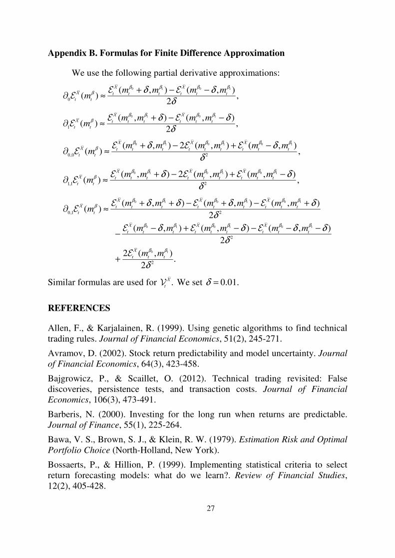
Table I

Mean and Variance Decompositions of Average Percentage Drift

This table presents the results of the mean and the variance decompositions of the average

percentage drift. The expected value of the average percentage drift, ,t

θ is denoted by ;t

m

tMɶ denotes the percentage composition of the basic component ;t

mɶ 0 1 01( , , )t t tM M M denote

the percentage compositions of the estimation risk adjustment components associated with 0 0 11 ,( , , ).t t tv v v

β β ββ The variance of the average percentage drift is denoted by ;t

v tVɶ denotes the

percentage composition of the basic component ;t

vɶ 0 1 01( , , )t t tV V V denote the percentage

compositions of the estimation risk adjustment components associated with 0 0 11 ,( , , ).t t tv v vβ β ββ

The results show that ignoring estimation risk does not materially bias the expected value of average percentage drift but materially underestimates its variance. The figures are measured in percent.

Panel A: Mean Decomposition Panel B: Variance Decomposition

mt Mt

0 Mt1 Mt

01 vt Vt0 Vt

1 Vt01

0t =

T 5 9.246 100.996 -0.028 4.523 -5.492 0.170 2.394 272.706 141.971 -317.070 10 9.218 101.522 -0.247 4.430 -5.705 0.164 1.238 283.437 147.039 -331.714 15 9.239 101.352 -0.206 4.523 -5.668 0.162 0.833 286.983 148.586 -336.401 20 9.259 101.173 -0.164 4.590 -5.599 0.161 0.630 289.006 149.615 -339.251

14

t T=

T 5 10.483 100.703 -0.027 3.867 -4.543 0.158 2.502 273.141 158.191 -333.834 10 11.248 100.650 -0.101 3.450 -3.999 0.141 1.174 293.917 171.028 -366.119 15 11.148 100.650 -0.027 3.303 -3.926 0.133 0.627 299.737 160.516 -360.881 20 12.099 100.529 -0.061 2.936 -3.405 0.120 0.285 309.165 179.205 -388.656

12

t T=

T 5 11.377 100.508 -0.076 3.315 -3.747 0.151 3.132 273.353 175.882 -352.368 10 12.134 100.487 -0.076 2.892 -3.303 0.124 0.818 299.676 181.614 -382.108 15 9.997 100.822 -0.099 2.918 -3.642 0.115 0.771 276.053 144.729 -321.552 20 10.358 100.418 -0.027 2.748 -3.138 0.102 0.503 280.635 161.321 -342.459

34

t T=

T 5 10.814 100.470 0.231 2.780 -3.480 0.167 3.766 234.774 103.979 -242.518 10 9.845 101.110 -0.140 2.587 -3.557 0.126 2.045 250.804 121.513 -274.361 15 10.234 100.277 0.049 2.704 -3.031 0.101 0.908 272.862 158.706 -332.477 20 9.742 100.204 0.021 2.579 -2.804 0.094 1.999 265.410 154.560 -321.969

251252

Tt =

T 5 13.348 100.000 0.000 0.000 0.000 0.157 0.000 219.977 319.977 -439.954 10 11.645 100.000 0.000 0.000 0.000 0.139 0.000 191.320 291.320 -382.640 15 11.412 100.000 0.000 0.000 0.000 0.122 0.000 185.458 285.458 -370.916 20 10.649 100.000 0.000 0.000 0.000 0.105 0.000 198.146 298.146 -396.292

32

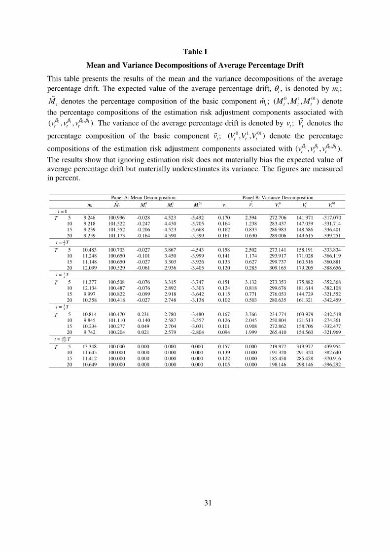
Table II

Horizon Effect and Hedging Demand against Estimation Risk

This table presents the optimal stock allocation, the suboptimal stock allocation, and their difference as the hedging demand against estimation risk. The optimal allocation is defined

by * 2( ) / [ 1( ( )])t t tm r T tvξ γσ γ− + −≡ − and the suboptimal allocation is defined by

2( ) / [ ( ( )]) ,1t t tvm r T tξ γσ γ− +≡ −−ɶ ɶɶ where γ and T are the investor’s risk-aversion

parameter and investment horizon. The hedging demand is defined by * .t t tξ ξ−∆ ≡ ɶ We

consider four investment horizons, 5,10,15,20,T = and present *( , , )t t tξ ξ ∆ɶ at five points of

time, namely ,t Tδ= 3 2511 14 2 4 252

0, , , , .δ = The results show that, at time 0,t = the optimal

allocation monotonically decreases with horizon, while the suboptimal allocation is not sensitive to the horizon. As the remaining horizon decreases, the hedging demand decreases and eventually becomes close to zero. The figures are measured in percent.

Optimal Strategy Suboptimal Strategy Difference

T 5 10 15 20 5 10 15 20 5 10 15 20

0t = γ 5 45.606 38.736 33.829 30.049 56.392 56.531 56.565 56.589 -10.787 -17.796 -22.736 -26.540

7 32.147 27.075 23.499 20.774 40.264 40.364 40.388 40.405 -8.118 -13.289 -16.890 -19.631 9 24.821 20.810 18.001 15.874 31.310 31.387 31.406 31.419 -6.489 -10.577 -13.405 -15.545

t = 1

4T

γ 5 55.548 54.121 49.116 50.645 64.691 69.889 69.263 75.714 -9.143 -15.768 -20.146 -25.069 7 39.290 38.052 34.377 35.346 46.195 49.909 49.465 54.076 -6.905 -11.857 -15.088 -18.730 9 30.394 29.341 26.442 27.146 35.924 38.813 38.469 42.057 -5.530 -9.472 -12.027 -14.911

t = 1

2T

γ 5 63.969 64.753 49.594 49.833 70.665 75.917 61.607 63.805 -6.696 -11.164 -12.013 -13.972 7 45.392 45.782 34.952 35.053 50.464 54.221 43.999 45.571 -5.072 -8.439 -9.047 -10.518 9 35.176 35.408 26.985 27.035 39.244 42.170 34.219 35.442 -4.068 -6.761 -7.234 -8.407

t = 3

4T

γ 5 63.103 55.407 56.918 52.733 66.888 60.765 62.899 59.421 -3.784 -5.359 -5.981 -6.688 7 44.901 39.355 40.387 37.366 47.770 43.399 44.925 42.436 -2.868 -4.043 -4.538 -5.070 9 34.849 30.515 31.297 28.934 37.151 33.752 34.940 33.002 -2.302 -3.237 -3.643 -4.069

t = 251

252T

γ 5 83.809 72.292 70.716 65.557 83.837 72.314 70.734 65.572 -0.028 -0.022 -0.018 -0.015 7 59.862 51.636 50.510 46.826 59.883 51.653 50.524 46.837 -0.022 -0.016 -0.014 -0.011 9 46.559 40.161 39.285 36.420 46.576 40.174 39.297 36.429 -0.017 -0.013 -0.011 -0.009

33

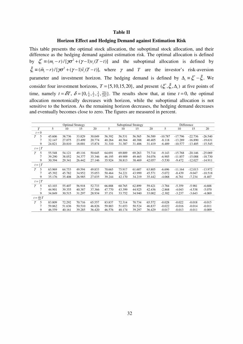
Table III

Average Market Timing Effect

This table presents the difference in the averages of | 1t tXξ = and | 0t tXξ = for the optimal

and the suboptimal allocations, *( , ),t t tξ ξ ξ= ɶ using the subsample period from 23rd December

1994 to 20th December 1999 ( 5 252× trading days), where 1tX = if the 1-day moving

average is above the 100-day moving average at time t and 0tX = otherwise. We use this

difference as a measure of the average effect of a buy signal ( 1)tX = on stock allocation. The

results show that, on average, the investor allocates an additional proportion of his wealth to the risky stock when a buy signal is observed. The average market timing effect is mild but economically significant. The figures are measured in percent.

Optimal Strategy Suboptimal Strategy Difference

T 5 10 15 20 5 10 15 20 5 10 15 20 γ 5 5.819 3.068 2.549 2.218 5.485 3.333 3.176 3.115 0.334 -0.265 -0.627 -0.897

7 4.151 2.169 1.789 1.547 3.917 2.381 2.268 2.225 0.234 -0.212 -0.480 -0.678 9 3.226 1.677 1.377 1.188 3.047 1.852 1.764 1.730 0.180 -0.175 -0.387 -0.543

34

Figure 2. Differences in average market timing effect between the optimal and the

suboptimal allocation strategies. This figure plots the difference in the average market timing effect between the optimal and the suboptimal allocations as a function of the investment horizon T and the risk-aversion parameter ,γ using the subsample period from

23rd December 1994 to 20th December 1999 ( 5 252× trading days). The results show that, except for the shortest horizon considered ( 5),T = the average market timing effect is

stronger for the suboptimal strategy. The differences are more notable as the horizon increases and the risk-aversion parameter decreases. The figures are measured in percent.

35

Table IV

Welfare Cost for Ignoring Estimation Risk

This table presents the welfare cost which measures the percentage wealth compensation required to leave the investor, who has $1 today to invest up to the horizon, indifferent between the optional and the suboptimal allocation strategies. We consider four investment

horizons, 5,10,15,20,T = and present the results at five points of time, namely ,t Tδ=3 2511 1

4 2 4 2520, , , , .δ = At time 0,t = the welfare cost is strongly increasing in horizon. For the

longer horizons, 15,20,T = the welfare cost remains above 3% for at least one quarter of

the horizons. The results show that it is costly for a long-horizon investor to ignore estimation risk. The figures are measured in percent.

T 5 10 15 20

t = 0 γ 5 0.530 3.434 9.954 21.474

7 0.426 2.730 7.829 16.644 9 0.352 2.245 6.394 13.467

t = 1

4T

γ 5 0.269 1.789 4.851 10.927 7 0.217 1.436 3.869 8.648 9 0.180 1.187 3.186 7.084

t = 1

2T

γ 5 0.091 0.540 0.992 1.859 7 0.074 0.436 0.797 1.495 9 0.061 0.362 0.660 1.237

t = 3

4T

γ 5 0.014 0.058 0.109 0.187 7 0.011 0.046 0.089 0.151 9 0.009 0.038 0.074 0.126

t = 251

252T

γ 5 0.000 0.000 0.000 0.000 7 0.000 0.000 0.000 0.000 9 0.000 0.000 0.000 0.000

36

Figure 3. Welfare cost for ignoring estimation risk at time zero. This figure plots the welfare cost as a function of the investment horizon T and the risk-aversion parameter γ at

time 0.t = The results show that the welfare cost increases with horizon at an increasing rate. Besides, the welfare cost increases as the risk-aversion parameter decreases and the increase is stronger for longer horizons. The figures are measured in percent.