Team 3 Final Report Boeing Blended Wing Body Project

16.100: Aerodynamics Fall 2003

Amy Brzezinski Tanya Cruz Garza

x_______________________ x_______________________

Julia Thrower Brady Young

x_______________________ x_______________________

Table of ContentsIntroduction................................................................................................................................................. 2Overview of Models Used........................................................................................................................... 2

Scaled Wind Tunnel ................................................................................................................................. 2Athena Vortex Lattice (AVL)................................................................................................................... 3Euler Computational Fluid Dynamics ...................................................................................................... 3

Section 1: Wind Tunnel Model .................................................................................................................. 41.1 Wind Tunnel Testing Procedure......................................................................................................... 41.2 Wind Tunnel Data Reduction ............................................................................................................. 41.3 AVL Procedure for Wind Tunnel Conditions .................................................................................. 101.4 Wind Tunnel Data Analysis.............................................................................................................. 13

Section 2: Athena Vortex Lattice Model................................................................................................. 242.1 Introduction to AVL ......................................................................................................................... 242.2 Approach Conditions without Flaps ................................................................................................. 242.3 Approach Conditions with Flaps ...................................................................................................... 242.4. Conclusion....................................................................................................................................... 34

Section 3: Fluent Model............................................................................................................................ 353.1 Fluent Assumptions .......................................................................................................................... 353.2 Fluent Methods ................................................................................................................................. 353.3 Convergence and Residuals.............................................................................................................. 363.4 Fluent Results and AVL Comparisons for Mach 0.50...................................................................... 373.5 Fluent Results and AVL Comparisons for Cruise at Mach 0.85 ...................................................... 393.6 Static Stability................................................................................................................................... 413.7 Fluent Results and AVL Comparisons for Cruise Angle-of-Attack at Varying Mach Number....... 41

Interim Conclusion ................................................................................................................................... 43Section 4: Redesign Strategy.................................................................................................................... 44

4.1 AVL Redesign Methods ................................................................................................................... 444.2 Fluent Redesign Methods ................................................................................................................. 454.3 Sensitivity Tests Results ................................................................................................................... 454.4 Final Design Decisions..................................................................................................................... 46

Section 5: Redesign Analysis Using AVL................................................................................................ 485.1 Approach Conditions with Flaps ..................................................................................................... 485.2 Cruise Condition Analysis with AVL.............................................................................................. 575.3 Conclusion ........................................................................................................................................ 57

Section 6: Fluent Model Analysis of Redesign........................................................................................ 586.1 Fluent Analysis Overview ................................................................................................................ 586.2 Fluent Results and AVL Comparisons for Redesign BWB Geometry Cruise at Mach 0.85 ........... 586.3 Static Stability................................................................................................................................... 616.4 Fluent Results and AVL Comparisons for Cruise Angle-of-Attack at Varying Mach Number....... 61

Final Conclusion........................................................................................................................................ 63Appendix A: Distribution of Tasks.......................................................................................................... 64Appendix B: Tables of Numerical Quantities........................................................................................ 65Appendix C: Design Team vs. Hammock ............................................................................................... 67Appendix D: Matlab Code for Fluent Graphs ....................................................................................... 68

1

IntroductionThe Blended Wing Body (BWB) is vehicle whose highly aerodynamic design intends to

maximize lift versus drag ratio and thus increase overall fuel efficiency. The main challenge of the BWB design, which resembles that of a flying wing, is stability. The vehicle lacks the typical configuration of control surfaces used in conventional aircraft, such as a rudder and elevator in a separate tail. Thus, it is important to determine the static stability of the BWB’sunique configuration, especially at approach and cruise conditions.

A low speed aerodynamic model of the BWB was created to evaluate these stability characteristics. Numerous methods of modeling aerodynamic flow are available and commonly used for this type of task, and in order to obtain the best possible model for our problem, a combination of several methods was applied and compared for consistency.

Overview of Models UsedThis project necessitated multiple methods of modeling the aerodynamic performance of

the BWB aircraft. Each of these models has its own merits and weaknesses. The methods used in this experiment were: scaled wind tunnel modeling, Athena Vortex Lattice (a computerizedvortex lattice method), and Euler Computational Flow Dynamics.

Scaled Wind Tunnel In the wind tunnel, a 1/47th scale model of the BWB was used. The airflow was

simulated by changing the angle of attack of the mock-up aircraft and measuring the various forces on it for freestream speeds of 50mph and 100mph. For this to be an accurate model, it is assumed that the geometry of the scaled down BWB is the same as the full sized airplane, and that the streamlines of the wind tunnel test follow this geometry in the same way that the streamlines flow around the actual aircraft.

To create an accurate model, it is necessary to match Mach number and Reynolds number with the desired flight situation. Unfortunately, due to the limits of our facilities, it was impossible to test at velocities higher than 100mph and were limited to using atmosphericpressure. Given unlimited resources, these parameters could be matched by pressurizing the tunnel, cooling the tunnel, or changing the fluid from air to a more viscous fluid.

However, for the purposes of this project, it is not necessary to match these valuesexactly. The Mach numbers tested are around .15 and therefore don't create wave drag at any point on the aircraft. The Reynolds numbers used are small enough that the viscous effects are relatively insensitive to moderate variation of Reynolds number. This means that the drag estimates from the wind tunnel are low, but not enough to make a noticeable difference in the experimental data.

The primary sources of error from the wind tunnel model stem from physical variations in the experiment's setup and execution. There are measurement errors and rounding errors associated with the load cell. The location of the model's attachment to the load cell must be very precisely measured in order to return accurate results, especially moments. The cylindricalsupport, as well as the balance arm and other appendages necessary for running the experiment,change the geometry of the BWB model. While significant effort to adjust the measurements to account for these variations was taken, their effect cannot be completely ignored. The wind tunnel itself is also not a perfect model of the atmosphere the actual BWB will experience, as there are wall effects, imperfect freestream flow, high temperatures, as well as others.

2

Athena Vortex Lattice (AVL) AVL is a computer program that uses 3D vortex lattice methods to simulate flow around

three dimensional bodies comprised of flat vortex panels. Because it uses vortex lattice methods,it assumes an incompressible, irrotational, inviscid flow. These assumptions limit it to calculating lift and induced drag only. AVL cannot determine viscous effects of a fluid, and likewise cannot simulate flow separation. This limits its usefulness to small angles of attack where there is little or no separation, and skin friction estimates must be made outside the program. Because it requires an incompressible flow, it is also only accurate at lower Mach numbers and becomes rapidly less accurate in the transonic and supersonic regions.

To account for the lack of skin friction, a rough estimate was performed outside of AVL using flat plate theory. Flat plate theory models the body in question as a flat plate parallel to the freestream flow. This has several limitations: it assumes that all properties of the flow are uniform across the plate (pressure, velocity, turbulent or laminar flow). This is certainly not the case with the BWB; the shape of the wing causes flow to go faster in some places than others, as well as many other irregularities. This also assumes totally attached flow. These assumptionscause the total estimates to be a little low.

Because the drag estimates are low and the lift estimates are optimistic, this would implythat moment coefficients are also higher than they should be.

Euler Computational Fluid Dynamics The final model done in Fluent, a Euler Computational Fluid Dynamics program. Similar

to AVL, it is a computerized flow simulator that models the flow around a 3D body. Unlike AVL, it only assumes an inviscid flow and is able to model compressible and rotational flows.

The usual constraining factor when fluent is being used is the accuracy of the body entered in the program. Because it is a numerical method using panels on the aircraft and cells in the surrounding flow, the precision of the model is directly related to how dense the mesh is.This is especially important in critical areas such as the leading edge, where a sharp edge is liable to trip turbulent flow and cause a suction peak, significantly increasing pressure drag. The trade-off with a high density mesh is the computing power necessary to carry out all of the calculations.

Unfortunately, due to the complexity of the equations involved, the iterative nature of the process, and the sheer number of cells to evaluate, CFD models take much longer to calculate than AVL (several hours as compared to a few seconds.) This makes CFD impractical to use for many tasks such as parameter optimization, where many solutions to the flow equations are required. Like AVL, it is unable to make skin friction estimates. This limits the usefulness of CFD to modeling the transonic and supersonic regions of the flow, regions where the accuracy of AVL breaks down. Through the subsonic region, AVL and CFD should return very nearly identical results, and because AVL is so much faster, it is usually the tool of choice. A more detailed comparison of AVL and CFD at cruise conditions is provided later in this text.

3

Section 1: Wind Tunnel Model

1.1 Wind Tunnel Testing Procedure With a Blended Wing Body (BWB) model, scaled to 1/47th of the actual aircraft, wind tunnel tests were conducted in the Wright Brothers Wind Tunnel. The experimental procedure involved a tuft flow visualization, an audio test, flow observation with a smoke wand, and force measurements on the model at varying velocities and angles of attack. First, for the tuft flow visualization, yarn tufts were arranged on the top surface of the BWB model. The wind tunnel airflow speed was set at 50 miles per hour, and the angle of attack of the model was inclined from 0 degrees to 16 degrees, in 2 degree increments. The tuft movement due to the flow behavior was observed as the angle of attack was varied. Secondly, an audio test was performedaround the BWB model body with a microphone, in order to detect areas of turbulence, indicated in the test by the presence of white noise. For the audio test, the angle of attack was once again varied from 0 degrees to 16 degrees, in 2 degree increments. The microphone was placed along the body surface, at the leading and trailing edges, and above the body surface. Next, a smokewand was used to observe the streamlines of the flow around the body. The angle of attack of the body was varied from 0 to 6 degrees, in 2 degree increments. The streamlines were observed over and behind the BWB model. Finally, force measurements were taken on the model at varied angles of attack for two velocities. Specifically, the forces of lift, drag, and pitching moment were measured. For the first velocity, 50 miles per hour, the angle of attack was first varied from -3 to 3 degrees in 1 degree increments, and then varied from 3 to 15 degrees in 2 degree increments. For the second velocity, 100 miles per hour, the model angle of attack was varied from -3 to 3 degrees in 1 degree increments, and then varied from 3 to 9 degrees in 2 degree increments. The values for the lift, drag, and pitching moment were recorded continuously for each angle of attack.

1.2 Wind Tunnel Data Reduction In order to analyze the wind tunnel results, the lift, drag, and pitching moment data needed to be corrected for errors and reduced to non-dimensional coefficients. First, the lift and drag forces were converted from millivolts, to Newtons, and the pitching moment was converted frommillivolts, to Newton meters. Next, the experimentally collected data points needed to be reduced from continuously collected data, to single averaged values for each distinct angle of attack. To do so, 30 data points were taken for each angle of attack from the converted measurements, within the regions of steady flow after the transient due to the angle of attack adjustments had settled out. The selected data points were then averaged for each angle of attack and each airflow velocity.

1.2.1. Experimental Parameters In order to correct for errors and evaluate the experimental results, several model and flow parameters were calculated. First, for the model itself, the location of the mean aerodynamicchord, c , of the BWB was estimated. The length of the mean aerodynamic chord was given in project documentation as a design parameter. In order to find the x and y coordinates for the mean aerodynamic chord leading edge, the AVL software was used. First, the x and y values for the chord lengths closest to the mean aerodynamic chord were recorded from the AVL BWB dimensions. See Figure 1.1 below.

4

BWB Wing Section

y

•(x1, y1)

Figure 1.1: BWB Wing Section Chord Analysis

Secondly, a linearization of the span location as a function of the chord length was created, written as

ccccyy

yyc 212

122 (Eq. 1.1)

Where c was substituted into the linearization to find the span location, y, for c . Next, a linearization of the leading edge x location as a function of the span was derived as

cc yyyyxx

xx 212

122 (Eq. 1.2)

Substituting the value forc

y found above into this equation produced the x location of the mean

aerodynamic chord leading edge, cx . The quarter chord point of the mean aerodynamic chord

was used as the quarter chord point for the entire BWB craft.

Next, flow parameters were derived. The air density for both 50 and 100 miles per hour was computed with the equation

RT

P (Eq. 1.3)

x

c2cc1

•(x , y )

•(x2, y2)c c

5

Where is the static pressure of the air flow, measured experimentally,P R is the specific gas

constant for air, and is the static temperature of the air flow, measured experimentally. Given the density, the dynamic pressure for both 50 and 100 miles per hour was calculated with the equation

T

2

2

1Vq (Eq. 1.4)

Where is air density, as calculated above, and is the airflow velocity. The Reynolds Number for both 50 and 100 miles per hour was also calculated with the equation

V

v

cVRe (Eq. 1.5)

Where is the freestream air velocity, V c is the mean aerodynamic chord, and is the kinematicviscosity for air at standard pressure and 85 degrees Fahrenheit.

v

1.2.2. Force Corrections

In order to obtain accurate results from the BWB Wind Tunnel test, corrections needed to be made to the drag and moment measurements. See Figure 1.2 below for a schematic of the modelsetup in the wind tunnel and the relevant model dimensions.

BWB Model

Balance Arm

BalanceSupportCylindrical

Support

bah

bal

babcylh

cyldbsh

bsl

Figure 1.2: BWB Wind Tunnel Model Setup

First, the drag measured in the tunnel included drag due to the cylindrical support, the balance arm, and the balance support, in addition to the drag force on the BWB model. Therefore, the total drag force on the BWB model was derived as follows:

bsbacstesttotal DDDDD (Eq. 1.6)

6

Where is the drag force experimentally measured in the wind tunnel, is the drag force

on the cylindrical support, is the drag force on the balance arm, and is the drag force on

the balance support.

testD csD

baD bsD

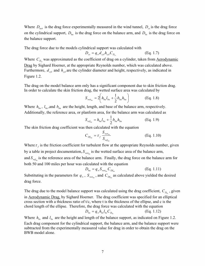
The drag force due to the models cylindrical support was calculated with

csDcylcylcs ChdqD (Eq. 1.7)

Where was approximated as the coefficient of drag on a cylinder, taken from AerodynamiccsDC

Drag by Sighard Hoerner, at the appropriate Reynolds number, which was calculated above.Furthermore, and are the cylinder diameter and height, respectively, as indicated in

Figure 1.2.cyld cylh

The drag on the model balance arm only has a significant component due to skin friction drag.In order to calculate the skin friction drag, the wetted surface area was calculated by

babababawet hblhSba 2

12 (Eq. 1.8)

Where , ,and are the height, length, and base of the balance arm, respectively.

Additionally, the reference area, or planform area, for the balance arm was calculated as bah bal bab

babababaref hblhSba 2

1(Eq. 1.9)

The skin friction drag coefficient was then calculated with the equation

ba

ba

ba

ref

wetfDf S

SC (Eq. 1.10)

Where f is the friction coefficient for turbulent flow at the appropriate Reynolds number, given

by a table in project documentation, is the wetted surface area of the balance arm,

and is the reference area of the balance arm. Finally, the drag force on the balance arm for

both 50 and 100 miles per hour was calculated with the equation

bawetS

barefS

baba Dfwetba CSqD (Eq. 1.11)

Substituting in the parameters for , , and as calculated above yielded the desired

drag force.

qbawetS

baDfC

The drag due to the model balance support was calculated using the drag coefficient, , given

in Aerodynamic Drag,bsDC

by Sighard Hoerner. The drag coefficient was specified for an elliptical cross section with a thickness ratio of t/c, where t is the thickness of the ellipse, and c is the chord length of the ellipse. Therefore, the drag force was calculated with the equation

bsDbsbsbs ClhqD (Eq. 1.12)

Where and are the height and length of the balance support, as indicated on Figure 1.2.

Each drag component for the cylindrical support, the balance arm, and the balance support were subtracted from the experimentally measured value for drag in order to obtain the drag on the BWB model alone.

bsh bsl

7

A correction also needed to be made to the moment measured in the wind tunnel testing. Due to the force of drag on the model cylindrical support, a moment component was generated. The drag per unit length along the cylindrical support was calculated by

csDcylcs CdqD' (Eq. 1.13)

Then the drag per unit length was integrated in order to obtain the moment as given by the equations

2

0'

2

1' cscscs

h

cs hDxdxDMcs

(Eq. 1.14)

Where is the height of the cylindrical support. The moment is negative because it is a

nose down moment, whereas the convention defines a nose up moment as positive. Therefore, the moment on the BWB can be calculated with the equation

csh csM

cstestbwb MMM (Eq. 1.15)

Where is the moment measured in the wind tunnel, is the moment acting on the

BWB model, and is the moment due to the drag on the cylindrical support.testM bwbM

csM

1.2.3. Calculation of Coefficients

After correcting for errors in the experimentally measured data, the coefficients of lift, drag, and moment could be calculated. First, the lift coefficient could be calculated with the equation

ref

testL Sq

LC (Eq. 1.16)

Where is the lift measured in the wind tunnel testing and is the reference, or planform,

area of the BWB model, given in the project documentation.testL refS

Next, given the lift coefficient, a correction was needed to be made to the angle of attack. The effective angle of attack in the wind tunnel is actually larger than the effective angle of attack in an unbounded flow. This disparity was due to an upwash effect from the wind tunnel walls.Several wind tunnel geometry parameters needed to be defined in order to specify the boundary correction factor, , for the wind tunnel. First, the aspect ratio of the tunnel was calculated, given by

W

H (Eq. 1.17)

Where H is the wind tunnel height, and W is the wind tunnel width. Additionally, the effective span to jet width ratio was defined by

W

bk e (Eq. 1.18)

Where W is the wind tunnel width, and is the effective span, given by eb

bbe 9. (Eq. 1.19)

Where b is the physical span of the BWB model. The parameters of and allowed the value

of the boundary correction factor, eb

, to be specified from a table in given project documentation. Another necessary parameter is the cross sectional area of the tunnel, given by

8

22HW

C (Eq. 1.20)

Where W is the wind tunnel width, and H is the wind tunnel height. The change in angle of attack induced by the upwash could then be quantified with the equation

Lref

i CC

S180 (Eq. 1.21)

Where180

is a unit conversion from radians to degrees, is the boundary correction factor

from above, and C is the tunnel cross sectional area. With this calculation for the change in the angle of attack, the angle of attack for the BWB model in an unbounded flow for the samecoefficient of lift can be obtained from the equation

itest (Eq. 1.22)

Where test is the angle of attack setting recorded from the wind tunnel testing. The effective

angle of attack was calculated for each tested angle of attack and corresponding coefficient of lift.

Next, the coefficient of drag was calculated for both 50 and 100 miles per hour. Using the total drag as calculated above, the total drag coefficient from the wind tunnel measurements was calculated with the equation

ref

totalD Sq

DC

total (Eq. 1.23)

Then, further calculations were made in order to correct for the induced drag decreases due to upwash effects caused by the wind tunnel walls. The change in induced drag was calculated with the equation

iLD CCi 180

(Eq. 1.24)

Where the numerical factor is a unit conversion of i from degrees to radians. Next, the final

coefficient of drag, including wind tunnel wall effects, was calculated with the equation

itotalfinal DDD CCC (Eq. 1.25)

Then, the coefficient of moment about the quarter chord was derived for each angle of attack, for both 50 and 100 miles per hour. First, the coefficient of moment about the model and cylindrical support joint was calculated from the experimental data as follows:

ref

bwbM Sq

MC

test (Eq. 1.26)

Where is the corrected moment value about the model and cylindrical support joint, is

the dynamic pressure, and is the reference area of the BWB model. In order to translate the

moment from the model and support joint and compute the coefficient of moment about the quarter chord, the following equation was used:

bwbM q

refS

c

xxCCC csc

LMM testc

4/4/

(Eq. 1.27)

9

Where is the x coordinate of the cylindrical support joint with respect to the nose of the

BWB model, is the x coordinate of the mean aerodynamic quarter chord point with respect

to the nose of the BWB model, and

csx

4/cx

c is the mean aerodynamic chord used to non-dimensionalize the x distance. Similarly, the moment about the aerodynamic center was calculated using Equation 1.27.

1.2.4. Center of Pressure and Aerodynamic Center

The center of pressure was calculated for the BWB model for each angle of attack. The center ofpressure is defined as the x coordinate on the aircraft where the pitching moment and the pitching moment coefficient are zero. For comparison and further analysis, the center of pressure for the model was non-dimensionalized by the quarter chord. The non-dimensionalizedcenter of pressure was calculated with the equation

L

Mccp

C

C

c

x

c

xc 4/4/ (Eq. 1.28)

Similarly, the aerodynamic center was calculated for the BWB at each angle of attack. The aerodynamic center is defined as the x coordinate on the aircraft about which the moment is constant with respect to changes in lift. In order to find the point where the moment is constantwith respect to lift, it was necessary to calculate the change of the moment coefficient with respect to the change in the lift coefficient. To find the derivative for a given alpha n , where

n,..., 21 are the consecutive values of alpha tested in the wind tunnel, a local linearization

around n was calculated to find the local slope about that angle, given by the equation

11

14/14/4/

nn

ncncc

LL

MM

L

M

CC

CC

dC

dC(Eq. 1.29)

Where and are the coefficients of moment for the angles of attack above and

below the angle of attack of concern, and the and are the coefficients of lift for the

angles of attack above and below the angle of attack of concern. Then, the non-dimensionalizedvalue for the aerodynamic center with respect to the nose of the BWB model was calculated by the equation

14/ ncMC14/ ncMC

1nLC1nLC

L

Mcac

dC

dC

c

x

c

xc 4/4/

(Eq. 1.30)

1.3 AVL Procedure for Wind Tunnel Conditions

AVL software was used to simulate the BWB aircraft flying at wind tunnel conditions for both 50 and 100 miles per hour. The resultant lift, drag, and moment coefficients were measured

10

through the AVL simulation. In the AVL software, the appropriate Mach number and angle of attack were specified, and the lift, drag, and moment coefficients for those conditions were calculated by the program. The Mach numbers corresponded to 50 and 100 miles per hour at standard pressure and temperature. The angles of attack used for the simulation were equivalent to those used in the experimental wind tunnel testing, varying from -3 to 3 degrees in 1 degree increments, and then from 3 to 15 degrees in 2 degree increments.

The coefficients of lift, drag, and moment were calculated in the AVL simulation and recorded.Since the AVL simulation is an inviscid model, the AVL drag results did not include a component of drag due to skin friction. Therefore, after the AVL results were obtained, the drag coefficient was corrected by adding a skin friction drag coefficient and a pressure drag coefficient.

y Geometry for Skin Friction Estimate

Figure 1.3: Geometry for Skin Friction Drag Estimate

The skin friction drag coefficient was approximated by dividing the wing of the BWB into two trapezoidal sections, as depicted in Figure 1.3, and then estimating the skin friction drag for each section. First, the chord lengths in each section were defined as functions of the spanwise location, given by the equations:

rm

rmi ly

y

llc (Eq. 1.31)

and

lr

lm

lt

x

li

lo

ci

co

ym

yt

11

mmmt

mto lyy

yy

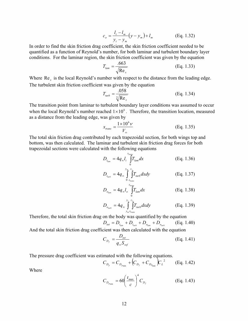
llc (Eq. 1.32)

In order to find the skin friction drag coefficient, the skin friction coefficient needed to be quantified as a function of Reynold’s number, for both laminar and turbulent boundary layer conditions. For the laminar region, the skin friction coefficient was given by the equation

x

lamTRe

663. (Eq. 1.33)

Where is the local Reynold’s number with respect to the distance from the leading edge.

The turbulent skin friction coefficient was given by the equation xRe

5 Re

058.

x

turbT (Eq. 1.34)

The transition point from laminar to turbulent boundary layer conditions was assumed to occur when the local Reynold’s number reached . Therefore, the transition location, measuredas a distance from the leading edge, was given by

6101

Vxtrans

6101 (Eq. 1.35)

The total skin friction drag contributed by each trapezoidal section, for both wings top and bottom, was then calculated. The laminar and turbulent skin friction drag forces for both trapezoidal sections were calculated with the following equations

trans

lam

x

lamii dxTlqD0

4 (Eq. 1.36)

m i

trans

turb

y c

x

turbi dxdyTqD0

4 (Eq. 1.37)

trans

lam

x

lamoo dxTlqD0

4 (Eq. 1.38)

t

m

o

trans

turb

y

y

c

x

turbo dxdyTqD 4 (Eq. 1.39)

Therefore, the total skin friction drag on the body was quantified by the equation

turblamturblam ooiitot DDDDD (Eq. 1.40)

And the total skin friction drag coefficient was then calculated with the equation

ref

totD Sq

DC

f (Eq. 1.41)

The pressure drag coefficient was estimated with the following equations.2

minminLDDDD CCCCC

Pfpp (Eq. 1.42)

Where

fp DD Cc

tC

4

max60min

(Eq. 1.43)

12

Where is the mean maximum thickness of the wing. Please see Appendix B for actual

values of the drag coefficients calculated in Maple using the process described above. maxt

The skin friction and pressure drag coefficients were added to the AVL drag result to obtain a corrected value of drag. The corrected drag could then be used in comparison with the experimental wind tunnel results. The AVL coefficient of moment result also required translation. The moment coefficient in the simulation was taken about the origin for the BWBdesign, and needed to be translated to the quarter chord point using the equation

c

xCCC c

LMM originc

4/4/

(Eq. 1.44)

Where is the coefficient of moment about the BWB origin, as given by AVL. originMC

1.4 Wind Tunnel Data Analysis

The results from both the experimental wind tunnel model and the theoretical AVL model can be compared to each other to evaluate the advantages and limitations of each model. To comparethe lift results, the coefficient of lift versus the angle of attack was plotted for each model.

Experimental Wind Tunnel Coefficient of Lift vs. Angle of Attack

-0.5

0

0.5

1

1.5

2

-5 0 5 10 15 20

Angle of Attack [deg]

Co

effi

cien

t o

f L

ift

(C_L

)

C_L for 50 mph C_L for 100 mph

Figure 1.4: Plot of Experimental Wind Tunnel Lift Data

As can be seen in Figure 1.4, the coefficient of lift for the experimental data follows a linear trend with respect to the angle of attack for angles below 9 degrees. Towards higher angles of attack, the graph resembles a more quadratic trend. This nonlinearity is due to the onset of stall as the angle of attack increases. Due to the viscosity of the flow, the flow begins to separate over the top of the wing surface at higher angles of attack, leading to a decrease in lift, observable in Figure 1.4.

13

AVL Wind Tunnel Coefficient of Lift vs. Angle of Attack

-0.5

0

0.5

1

1.5

2

2.5

-4 -2 0 2 4 6 8 10 12 14 16

Angle of Attack [deg]

Co

effi

cien

t o

f L

ift

(C_L

)

C_L for 50mph C_L for 100 mph

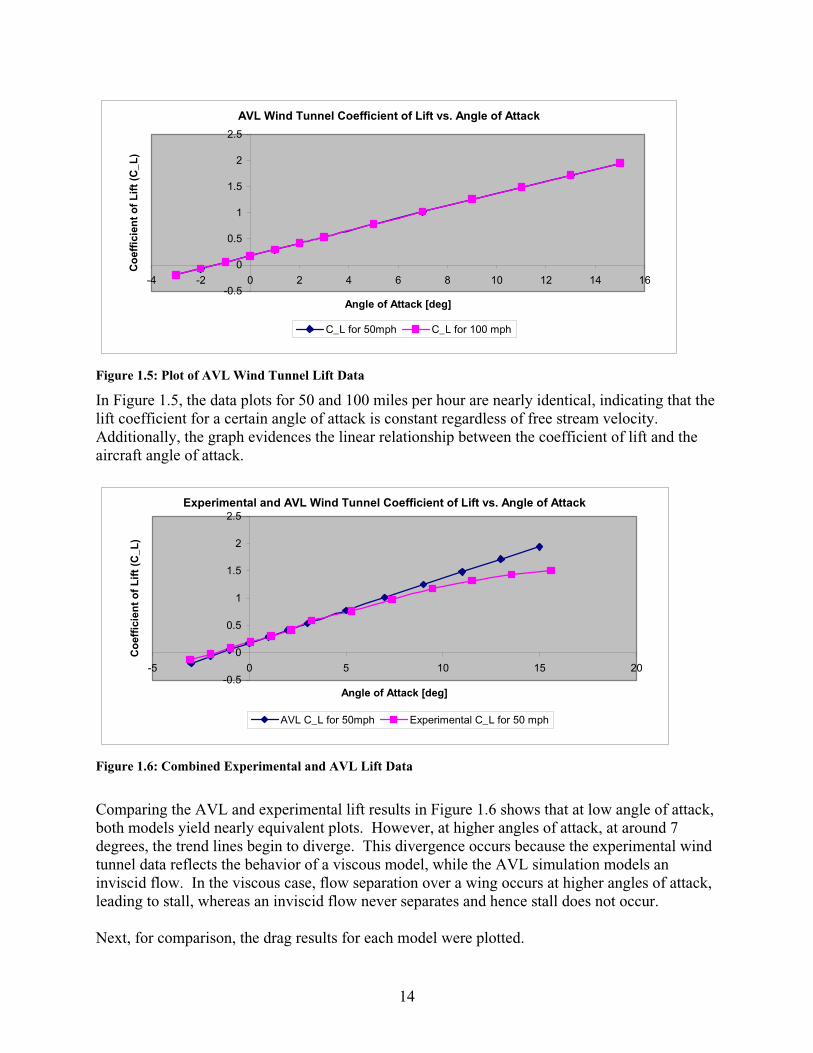
Figure 1.5: Plot of AVL Wind Tunnel Lift Data

In Figure 1.5, the data plots for 50 and 100 miles per hour are nearly identical, indicating that the lift coefficient for a certain angle of attack is constant regardless of free stream velocity.Additionally, the graph evidences the linear relationship between the coefficient of lift and the aircraft angle of attack.

Experimental and AVL Wind Tunnel Coefficient of Lift vs. Angle of Attack

-0.5

0

0.5

1

1.5

2

2.5

-5 0 5 10 15 20

Angle of Attack [deg]

Co

effi

cien

t o

f L

ift

(C_L

)

AVL C_L for 50mph Experimental C_L for 50 mph

Figure 1.6: Combined Experimental and AVL Lift Data

Comparing the AVL and experimental lift results in Figure 1.6 shows that at low angle of attack, both models yield nearly equivalent plots. However, at higher angles of attack, at around 7 degrees, the trend lines begin to diverge. This divergence occurs because the experimental wind tunnel data reflects the behavior of a viscous model, while the AVL simulation models an inviscid flow. In the viscous case, flow separation over a wing occurs at higher angles of attack, leading to stall, whereas an inviscid flow never separates and hence stall does not occur.

Next, for comparison, the drag results for each model were plotted.

14

Experimental Wind Tunnel Drag Polar

-0.5

0

0.5

1

1.5

2

0 0.05 0.1 0.15 0.2 0.25 0.3 0.35 0.4

Drag Coefficient (C_D)

Lif

t C

oef

fici

ent

(C_L

)

50 mph 100 mph

Figure 1.7: Experimental Wind Tunnel Drag Coefficient

Figure 1.7 shows the relationship between the lift coefficient and the drag coefficient for the BWB in the wind tunnel model. At lower angles of attack, the coefficient of drag does not change dramatically with the coefficient of lift, but as the angle of attack increases, the drag coefficient increases at a faster rate than the lift coefficient increases. The drag polar is significant in that the ideal operating angle of attack can be obtained for maximum lift with minimum drag, where the slope of the lift coefficient curve with respect to the drag coefficient is maximum. From these results, that point occurs around where the lift coefficient is .15 and the drag coefficient is around .025, at an angle of attack around 1 degree. Comparing the results of the 50 and 100 mph results, the 100 mph drag coefficient is greater than the 50 mph drag coefficient at lower angles of attack, where the force measurements in the wind tunnel were mostaccurate. This result is not consistent with theoretical drag coefficients compared at different speeds. In theory, the drag coefficient should decrease as the freestream velocity and the Reynold’s number increases. The wind tunnel results do not match theoretical concepts due to error in the data reduction. Approximations for the drag components due to the balance arm,balance support, and cylindrical support were not exact, and therefore the final reduced BWBdrag was slightly erroneous.

15

AVL Wind Tunnel Drag Polar

-0.5

0

0.5

1

1.5

2

2.5

0 0.05 0.1 0.15 0.2 0.25

Coefficient of Drag (C_D)

Co

effi

cien

t o

f L

ift

(C_L

)

C_D for 50 mph C_D for 100 mph

Figure 1.8: AVL Wind Tunnel Drag Polar

Figure 1.8 accurately shows that the lift and drag coefficients are independent of the free streamvelocity. As high angles of attack are approached, the drag coefficient changes at an increasingly faster rate relative to the change in lift.

Combined Experimental and AVL Drag Polar

-0.5

0

0.5

1

1.5

2

2.5

0 0.05 0.1 0.15 0.2 0.25 0.3 0.35 0.4

Coefficient of Drag (Cd)

Co

effi

cien

t o

f L

ift

(Cl)

AVL for 50 mph Experimental for 50 mph

Figure 1.9: Combined Experimental and AVL Drag Polar

When the lift and drag coefficient results for both models are plotted together as in Figure 1.9, at low angles of attack, the data is well matched. However, at higher angles of attack, disparity in both the lift and drag is revealed. As seen in the plots for the coefficient of lift versus angle of attack, at higher angles the lift in the experimental model is not as high as for the AVL modeldue to the absence of stall in the AVL model. Also due to stall, the drag coefficient for the experimental model is larger than that for the AVL model at high angles of attack. The drag coefficients may also differ due to approximations made in the reduction of the experimentalwind tunnel data. For example, the drag on the cylindrical support, the balance arm, and the balance support may have been underestimated. Therefore the final drag coefficient data for the wind tunnel experiment may contain some drag due to components of the wind tunnel setup

16

other than the BWB model itself. However, in any case, the drag on components other than the model itself are relatively small, and would not cause too great of an offset in final results ifestimated slightly inaccurately.

Experimental Wind Tunnel Quarter Chord Moment Coefficient vs. Coefficient of Lift

-0.2

0

0.2

0.4

0.6

0.8

1

-0.5 0 0.5 1 1.5 2

Coefficient of Lift (C_L)

Co

effi

cien

t o

f M

om

ent

(C_M

)

50 mph 100 mph

Figure 1.10: Experimental Wind Tunnel Quarter Chord Moment Plot

Figure 1.10 shows that the coefficient of moment is linearly proportional to the coefficient of lift.The pitching moment is caused by the lift distribution, so this relationship makes sense.

AVL Quarter Chord Moment Coefficient vs. Coefficient of Lift

-0.2

0

0.2

0.4

0.6

0.8

1

-0.5 0 0.5 1 1.5 2 2.5

Coefficient of Lift (C_L)

Co

effi

cien

t o

f M

om

ent

(C_M

) at

c/4

50 mph 100 mph

Figure 1.11: AVL Wind Tunnel Quarter Chord Moment Plot

Figure 1.11 confirms the linear relationship between the coefficient of moment and the coefficient of lift, and that the coefficient of moment and coefficient of lift are independent of air speed.

17

Experimental and AVL Quarter Chord Moment Coefficients, 50 mph

-0.2

0

0.2

0.4

0.6

0.8

1

-0.5 0 0.5 1 1.5 2 2.5

Coefficient of Lift (Cl)

Co

effi

cien

t o

f M

om

ent

(C_M

)at

c/4

AVL Experimental

Figure 1.12: Combined Experimental and AVL Moment Plot

Figure 1.12 shows a similar slope for the experiment and AVL coefficient of moment plots.Also, some disparity in magnitude is evident between the two lines. The experimentalcoefficient of moment is slightly higher than the AVL coefficient of moment. This error is partially due to the presence of upwash induced by the wind tunnel walls which are not part of the AVL model. Additionally, there may be error in the estimation of the moment on the cylindrical support due to drag, causing the total moment estimation to be higher than actual.

Experimental Wind Tunnel Aerodynamic Center Moment Coefficient vs.Coefficient of Lift

0

0.05

0.1

0.15

0.2

0.25

0.3

0.35

0.4

0.45

0.5

-0.4 -0.2 0 0.2 0.4 0.6 0.8 1 1.2 1.4 1.6Coefficient of Lift (C_L)

Co

effi

cien

t o

f M

om

ent

(C_M

_Xac

)

50 mph 100 mph

Figure 1.13: Experimental Aerodynamic Center Moment Plot

Figure 1.13 plots the moment coefficient about the aerodynamic center for the experimental wind tunnel results. The moment is positive, indicating stability. As the coefficient of lift increases, the moment coefficient increases, and therefore the BWB margin of stability increases. The values for the 100 mph data are smaller than that for the 50 mph data. This disparity is due to error in the moment data. Since the cylindrical support about which the moment force was measured was very close to the aerodynamic center, the actual recording of the data was not very

18

accurate. Additionally, the moment due to drag on the cylindrical support was not estimatedperfectly, causing error in the final results.

AVL Aerodynamic Center Moment Coefficient vs. Coefficient of Lift

-0.09

-0.08

-0.07

-0.06

-0.05

-0.04

-0.03

-0.02

-0.01

0-0.5 0 0.5 1 1.5 2 2.5

Coefficient of Lift (Cl)

Co

effi

cien

t o

f M

om

ent

(C_M

_Xac

)

50 mph 100 mph

Figure 1.14: AVL Aerodynamic Center Moment Plot

In Figure 1.14, the coefficient of moment about the aerodynamic center was plotted for the AVL data results. The results for the 50 and 100 mph conditions are nearly identical. Since the moment coefficient is negative, the BWB is unstable at all angles of attack. Around the coefficient of lift for which lift is equal to weight, the slope of the plot becomes zero. This occurs due to the fact that the aerodynamic center is defined as the point where the change in moment with respect to lift is constant.

Experimental and AVL Aerodynamic Center Moment Coefficients, 50 mph

-0.2

-0.1

0

0.1

0.2

0.3

0.4

0.5

-0.5 0 0.5 1 1.5 2 2.5

Coefficient of Lift (Cl)

Co

effi

cien

t o

f M

om

ent

(C_M

_Xac

)

AVL Experimental

Figure 1.15: Combined Experimental and AVL Moment Plot

The combined plot of experimental and AVL data in Figure 1.15 shows a great disparity between the two sets of data. This difference is due to the error inherent in the experimental momentdata, as mentioned previously.

19

The center of pressure and aerodynamic center was calculated for both the experimental and AVL models, as plotted below.

Experimental Center of Pressure and Aerodynamic Centervs. Coefficient of Lift, 50 mph

00.5

11.5

22.5

33.5

44.5

-0.5 0 0.5 1 1.5 2Coefficient of Lift (C_L)

Lo

cati

on

/ C

ho

rd L

eng

th(x

_cp

/c,

x_ac

/c)

Center of Pressure, 50 mph Aerodynamic Center, 50 mph

Figure 1.16: Experimental Center of Pressure and Aerodynamic Center

Figure 1.16 indicates that the center of pressure spikes about the point of zero lift, as expected.For lower values of lift, the aircraft is unstable in that the center of pressure is behind the aerodynamic center. However, at higher angles of attack, the center of pressure moves ahead of the aerodynamic center and is therefore stable. The plot of the aerodynamic center is nearly horizontal, as expected, since for a given wing configuration, the aerodynamic center location is constant with respect to changes in lift.

AVL Center of Pressure and Aerodynamic Center vs. Coefficient of Lift, 50 mph

0

0.5

1

1.5

2

2.5

3

3.5

4

-0.5 0 0.5 1 1.5 2 2.5Coefficient of Lift (C_L)

Lo

cati

on

/ C

ho

rd L

eng

th(x

_cp

/c, x

_ac/

c)

Aerodynamic Center Center of Pressure

Figure 1.17: AVL Center of Pressure and Aerodynamic Center

20

Figure 1.17 of the AVL data has more consistent trends. For positive lift, the aircraft is unstable in that the center of pressure is behind the aerodynamic center. The aerodynamic center is clearly constant across changes in lift coefficient.

Experimental and AVL Center of Pressure, 50 mph

1.5

2

2.5

3

3.5

4

4.5

-0.5 0 0.5 1 1.5 2 2Coefficient of Lift (Cl)

Lo

cati

on

/ Ch

ord

Len

gth

(x_

cp/c

)

.5

AVL Experimental

Figure 1.18: Experimental and AVL Center of Pressure

Figure 1.18 shows similar center of pressure locations away from the point of zero lift, where thecenter of pressure spikes in magnitude. The difference between the plots is due to the differences in the moment coefficients between the experimental and AVL models.

Experimental and AVL Aerodynamic Center, 50 mph

1

1.5

2

2.5

3

3.5

-0.5 0 0.5 1 1.5 2 2.5Coefficient of Lift (Cl)

Lo

cati

on

/ C

ho

rdL

eng

th(x

_ac/

c)

AVL Experimental

Figure 1.19: Experimental and AVL Aerodynamic Center

The aerodynamic center for the experimental and AVL results are nearly equivalent in value, as depicted in Figure 1.19.

21

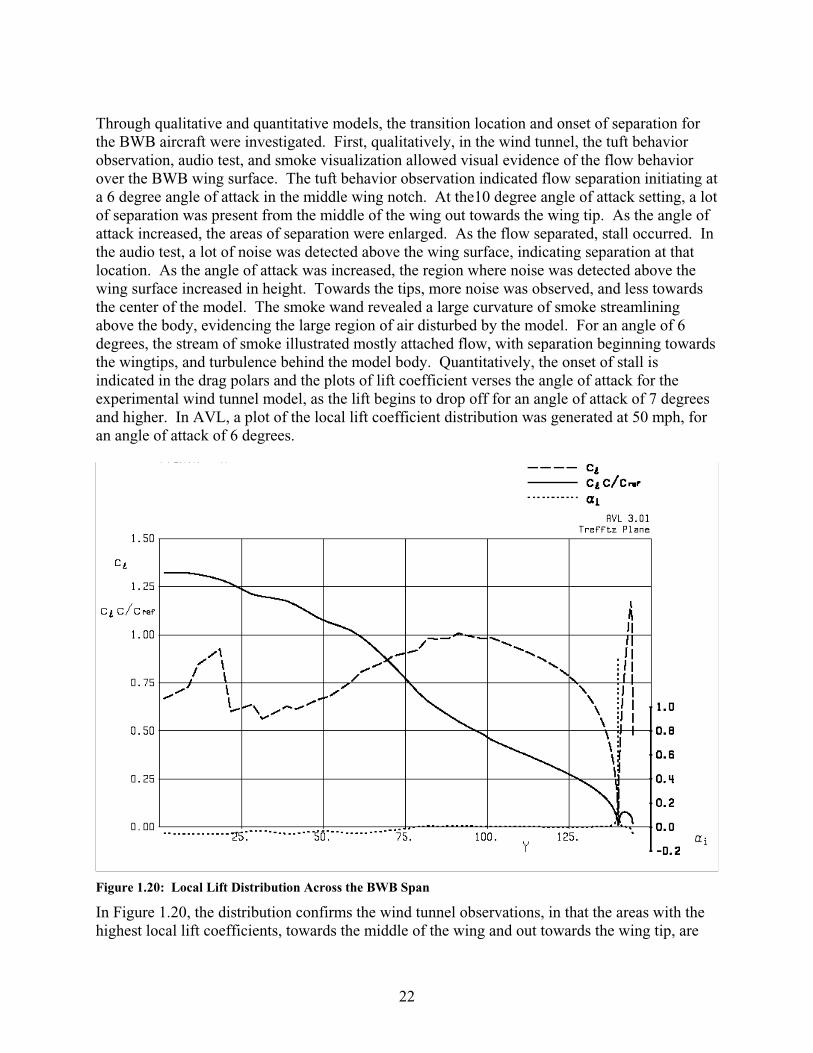
Through qualitative and quantitative models, the transition location and onset of separation for the BWB aircraft were investigated. First, qualitatively, in the wind tunnel, the tuft behavior observation, audio test, and smoke visualization allowed visual evidence of the flow behavior over the BWB wing surface. The tuft behavior observation indicated flow separation initiating at a 6 degree angle of attack in the middle wing notch. At the10 degree angle of attack setting, a lotof separation was present from the middle of the wing out towards the wing tip. As the angle ofattack increased, the areas of separation were enlarged. As the flow separated, stall occurred. In the audio test, a lot of noise was detected above the wing surface, indicating separation at that location. As the angle of attack was increased, the region where noise was detected above the wing surface increased in height. Towards the tips, more noise was observed, and less towards the center of the model. The smoke wand revealed a large curvature of smoke streamliningabove the body, evidencing the large region of air disturbed by the model. For an angle of 6 degrees, the stream of smoke illustrated mostly attached flow, with separation beginning towardsthe wingtips, and turbulence behind the model body. Quantitatively, the onset of stall is indicated in the drag polars and the plots of lift coefficient verses the angle of attack for the experimental wind tunnel model, as the lift begins to drop off for an angle of attack of 7 degrees and higher. In AVL, a plot of the local lift coefficient distribution was generated at 50 mph, for an angle of attack of 6 degrees.

Figure 1.20: Local Lift Distribution Across the BWB Span

In Figure 1.20, the distribution confirms the wind tunnel observations, in that the areas with the highest local lift coefficients, towards the middle of the wing and out towards the wing tip, are

22

the areas where the onset of flow separation was observed. In conclusion, the qualitative and quantitative results from the wind tunnel testing and from AVL are well correlated, in that the onset of stall begins in the middle notch of the wing and at the wing tip, at around a 7 degree angle of attack. The separation regions increase in size above and on the wing surface as the angle of attack increases, mostly occurring towards the wingtips before towards the root of the wing.

23

Section 2: Athena Vortex Lattice Model

2.1 Introduction to AVLAs discussed earlier, AVL is a vortex lattice program that can quickly calculate lift and

induced drag along any given wing, however it is unable to simulate viscous or high Mach number flows. This prevents it from accurately simulating cruise conditions of the BWB, but it is ideally suited for simulating slower speed situations, such as approach. It is also equipped to calculate the local cl at any point along the wing. If the cl of separation is determinedexperimentally, then AVL can be used to predict when and where separation and stall begin, despite the fact that AVL assumes an attached flow.

Approach for landing flight provides unique requirements and conditions for any type of aircraft. This is especially true for the BWB due to its blended aerodynamic design. The mostimportant considerations for approach flight are the speed of approach, the angle of approach for trimmed flight, the stall angle, and the static stability of the BWB. In order to analyze how the BWB stabilizes at approach conditions, various AVL simulations were run that examined the BWB performance without flaps and with flaps.

2.2 Approach Conditions without Flaps Before approach conditions with flaps were considered, AVL simulations of the BWB

without flaps were run. These simulations were run at Mach .2328 with varying angle of attack from –3 degrees to 15 degrees. The stall angle was determined by the angle at which a sectional coefficient of lift just equaled 1.6 (simulating a BWB with slats). The stall angle of attack for these conditions was found at around 10 degrees, with a coefficient of lift of 1.373. Using equation (1) where L=2 950 000 N (dry weight+ max payload + 25% fuel remaining), 225.1

kg/m , S= 728.36 m , and =1.3732 2LC

Lstall CSvL 2

2

1 (Eq. 2.1)

a stall velocity of = 69.39 m/s was calculated. However, one of the approach constraints is

that the maximum approach speed be 77.2 m/s (150 knots) and that this approach speed be 1.3* . With the stall speed calculated above, the approach speed would have to be 90.21 m/s,

which exceeds the maximum approach speed. From equation (1), it can be seen that in order to lower the stall speed, a larger coefficient of lift is needed. A larger coefficient of lift can be achieved by manipulating the flaps on the BWB.

Stallv

stallv

2.3 Approach Conditions with Flaps

2.3.1. Flap Correlation Between BWB and AVL In order to determine the flap correlations between the BWB and the AVL model, a

diagram of the BWB was measured with a ruler and the lengths of the flaps were recorded.Then, the total length of all the flaps was added and divided by fourteen in order to find the length of each evenly spaced AVL flap. Then, by examination between the BWB flap lengths and the AVL flap length, flap numbers from AVL were assigned to flap numbers on the BWB.

24

Table 2.1 displays the flap assignments between the BWB and AVL, with flap one being closest to the center of the plane.

BWB Flap # (As measured from center outward toward winglet)

AVL Flap # (As measured from centeroutward toward winglet)

1 1-22 3-73 8-94 10-125 136 14

Table 2.1: Flap correlations between BWB and AVL model

2.3.2. Optimal Flap Settings and Stall Conditions Optimal flap settings were calculated from the operating condition specifications and

constraints for approach conditions. Stall conditions were first examined. From the conditions of a maximum approach speed =77.2 m/s (150 knots, mach .2328) and =1.3*

(for safety), a maximum stall speed of =59.6 m/s (115.83 knots, mach .179) was found. By

assuming that lift equals total weight of the BWB (with payload and remaining fuel), and by using (Eq. 2.1) with the same variable values as before, along with =59.6 m/s, it is found

that . This coefficient of lift is the minimum value at which the two approach

speed conditions will be fulfilled.

approachv approachv Stallv

Stallv

Stallv

829.1stallLC

In order to find the necessary flap settings to fulfill the approach speed conditions, theminimum coefficient of lift ( ) for stall conditions was entered into the computer

program AVL, along with a stall Mach number of .179 (59.6 m/s). AVL generated a plot showing the sectional coefficient of lifts for the span of the BWB. Figure 2.1 shows the sectional coefficient of lift values on approach at stall conditions without flaps.

829.1stallLC

25

Figure 2.1: Sectional coefficient of lift at stalled approach conditions without flap deflection

Some of these sectional coefficients of lift were greater than =1.6, the requirement of

maximum sectional coefficient of lift with slats before stall of the BWB occurs. Slats are additional physical appendages added to the front of aircraft wings in order to eliminate suctionpeak at the leading edge, decrease drag, and increase allowable sectional coefficient of lift beforestall occurs. Places where the sectional coefficients of lift were especially large were around where BWB flaps three and four were. The flaps on the BWB were manipulated until the sectional coefficients of lift were all less than or equal to 1.6. At this point, the angle of attack for stall conditions was calculated as

lc

stall =18.67 o . Table 2.2 gives the flap settings for the

BWB in order to satisfy minimum stall speed and approach speed.

BWB Flap # (As measured from center outward toward winglet)

Angle of Flap Deflection(In Degrees)

1 -82 03 -234 -195 -106 -3

Table 2.2: Flap settings for BWB approach conditions.

As seen from the table, the flaps are set at negative values, meaning that they are deflected upwards with respect to the body of the BWB. Upward flaps contribute to the static

26

stability of the BWB as it approaches for landing by causing the center of pressure to move closer to the nose.

2.3.3. Trim ConditionsTrim conditions for the BWB with flaps deflected were found by using equation (2.1)

with values of L=2 950 000 N (dry weight+ max payload + 25% fuel remaining), 225.1

kg/m , S= 728.36 m , and =77.2 m/s. By solving for coefficient of lift, a value of

and

2 2approachv

085.1trimLC trim =12.06 o was found.

2.3.4. Coefficient of LiftFigure 2.2 shows the coefficient of lift versus angle of attack for approach conditions with flaps deflected. Stall and trim conditions are also highlighted.

Approach Conditions with Flaps: Cl vs. Angle of Attack

-1

-0.5

0

0.5

1

1.5

2

2.5

-5 0 5 10 15 20 25

Angle of Attack (degrees)

Co

effi

cien

t o

f L

ift

(Cl)

AVL data points collected for approach conditions w ith f laps Stall Trim

Figure 2.2: Coefficient of lift vs. angle of attack for approach conditions of BWB with flaps deflected.

Upon first view of this graph, it may seem strange that the angles of attack for stall and trim conditions are so high. However, when it is considered that the BWB is coming in forapproach with flaps deflected upwards in order to pitch the nose up, these values of alpha makesense. A good analogy to the BWB to think of when considering approach conditions is the space shuttle. The space shuttle, although not entirely like the BWB, does have a delta wing andthus can be viewed more as like the BWB than standard tube and wing designs of current commercial aircraft. As the shuttle approaches for landing, it flies at a high angle of attack, in order to keep stability and to use drag to help decrease its speed. This is the similar reason why the BWB has high angles of attack for approach trim and stall conditions.

2.3.5. Drag Polar Figure 2.3 shows the drag polar of the BWB with flaps deflected for approach conditions.

The two plots in the figure are of a drag polar just considering induced drag from AVL simulations and a drag polar including a skin friction drag estimate. This skin friction drag

27

estimate was calculated using the same flat plate approximation methods as explained in the wind tunnel section of this report. A final skin friction drag coefficient value of =.002535

was calculated and added to the induced drag coefficient in order to obtain the total coefficient ofdrag values. Pressure drag was neglected as its contributions to total drag were negligible as compared to other contributors. Wave drag was also neglected due to the low mach number at approach conditions. Stall and trim points considering total drag coefficients are noted in the figure.

fDC

Approach Conditions w ith flaps: Drag Polar

-1

-0.5

0

0.5

1

1.5

2

2.5

0 0.05 0.1 0.15 0.2 0.25

Coe f f i c i e nt of Dr a g ( Cd)

AVL induced drag AVL induced drag plus skin friction estimate Stall Trim

Figure 2.3: Drag polar for approach conditions of BWB with flaps deflected.

2.3.6. Moment Coefficient The moment coefficient about the trim aerodynamic center versus the coefficient of lift of

the BWB at approach conditions with flaps deflected is shown in Figure 2.4.

28

Approach Conditions with Flaps: Xac Moment vs. Cl

0

0.05

0.1

0.15

0.2

0.25

0.3

0.35

0.4

-1 -0.5 0 0.5 1 1.5 2 2.

Coefficient of Lift (Cl)

Mo

men

t C

oef

fici

ent

(Cm

) at

c/4

5

AVL data points collected for approach conditions with flaps Stall Trim

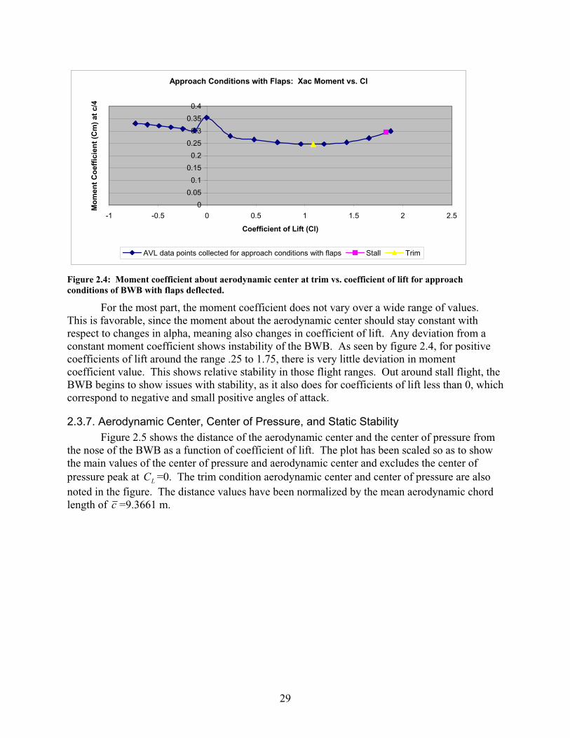
Figure 2.4: Moment coefficient about aerodynamic center at trim vs. coefficient of lift for approachconditions of BWB with flaps deflected.

For the most part, the moment coefficient does not vary over a wide range of values.This is favorable, since the moment about the aerodynamic center should stay constant with respect to changes in alpha, meaning also changes in coefficient of lift. Any deviation from a constant moment coefficient shows instability of the BWB. As seen by figure 2.4, for positive coefficients of lift around the range .25 to 1.75, there is very little deviation in momentcoefficient value. This shows relative stability in those flight ranges. Out around stall flight, the BWB begins to show issues with stability, as it also does for coefficients of lift less than 0, which correspond to negative and small positive angles of attack.

2.3.7. Aerodynamic Center, Center of Pressure, and Static StabilityFigure 2.5 shows the distance of the aerodynamic center and the center of pressure from

the nose of the BWB as a function of coefficient of lift. The plot has been scaled so as to show the main values of the center of pressure and aerodynamic center and excludes the center of pressure peak at =0. The trim condition aerodynamic center and center of pressure are also noted in the figure. The distance values have been normalized by the mean aerodynamic chord length of

LC

c =9.3661 m.

29

Approach with Flaps: Xac and Xcp

0

1

2

3

4

5

-1 -0.5 0 0.5 1 1.5 2 2

Coefficient of Lift (Cl)

Dis

tan

ce f

rom

No

se

.5

Xac from nose Xcp from nose Trim Xac Trim Xcp

Figure 2.5: Aerodynamic center and center of pressure vs. coefficient of lift for approach conditions of BWBwith flaps deflected.

As discussed in the wind tunnel section, the non-dimentionalized coefficient of pressure is calculated by the equation

L

Mccp

C

C

c

x

c

xc 4/4/ (Eq. 1.29)

and the non-dimensionalized aerodynamic center is calculated by

L

Mcac

dC

dC

c

x

c

xc 4/4/ (Eq. 1.31)

By definition, the center of pressure is the point at which the net moment on the BWB is equal to zero. The aerodynamic center is defined as the location where the net moment on the BWB is constant with respect to changes in angle of attack. The relative relation in positionbetween these two quantities determines if an aircraft is stable.

The large peak in center of pressure (x ) occurs around =3 and is due to the net lift

on the BWB approaching zero. As seen by Eq. 1.29, if is very small, the term /

becomes very large and therefore the distance of the center of pressure from the nose of the BWB becomes very large. In this case, the center of pressure has actually left the body. The aerodynamic center tends to stay constant as coefficient of lift values change. This makes sense, as the definition of the aerodynamic center is the point at which the moment is constant with respect to changes in angle of attack, and the coefficient of lift is dependent on angle of attack.

cp LC o

LC4/cMC LC

30

The BWB is statically stable if the center of pressure is at least a distance of 5% of the mean aerodynamic chord away from the aerodynamic center in the direction of the nose. For stability to occur, the center of pressure must be closer to the nose than the aerodynamic center.In general, aircraft tend to be more stable around higher angles of attack. As seen by figure 2.5, the BWB is unstable for angles of attack from -3 to 3 degrees due to the fact that the aerodynamic center is ahead of the center of pressure. For angles of attack greater than 3 degrees, the coefficient of pressure is ahead of the aerodynamic center.

At a trimmed approach with flaps, the location of the BWB’s center of pressure is at 2.433, as normalized by the mean aerodynamic chord ( c =9.3661 m). The location of the aerodynamic center at this condition is 2.670. In order for the BWB to be statically stable, there must be a distance of at least 5% of the mean aerodynamic chord between and x cp , with x

ahead of . Because the above values are non-dimensionalized, in order for the BWB to be

statically stable, there must be a difference of at least .05 between and x . By subtracting

x cp from , a static margin of .237 or 23.7% is found.

acx cp

acx

acx cp

acx

2.3.8. Lift Distribution

2.3.8.1. Approach at Trim ConditionsFigure 2.6 shows the span loading and sectional coefficient of lift distribution for the

BWB at trimmed approach conditions on half of the body. It may be assumed that this distribution is symmetrical for the whole body.

31

Figure 2.6: Span loading and sectional coefficient of lift vs. span length for approach conditions of BWB withflaps deflected at trim.

The dashed line is the sectional coefficient of lift ( ) distribution. This distribution

gives the coefficient of lift at each span location of the wing by examining the chord length and the conditions on that section of the wing. It is evident from the plot that the sectional coefficients of lift are well within the constraint of being less than 1.6 (with slats on the BWB).The flaps have a “leveling affect,” meaning that the sectional coefficient of lift is fairly similarfor each span section. At the end of the wing, the sectional coefficient of lift falls off to zero, this satisfying the boundary condition at that point. The large peak in near the edge of the

wing is due to the winglet, and was not considered as part of the requirement of less than 1.6.

lc

lc

lc

The solid line in figure 2.6 is the span loading on the wing. Span loading is the amountof weight a wing section of span supports. As seen by the figure, the BWB is loaded most around the root of the wing, with wing loading decreasing as the wing is traveled out towards the tips. This is favorable because if too much load is placed more on the outward areas of the BWB,more stresses will occur near the center sections, thus causing problems with structural strength.Near the outer half of the span, span loading becomes more uniform, thus preventing any excessive bending moments and increasing stability. Loading at the end of the wing falls to zero, thus satisfying the boundary condition, and there is only a small amount of loading on the wingtip.

32

The lift over drag ratio at trimmed approach conditions with flaps can be calculated by finding the ratio of the coefficient of lift over the coefficient of drag. With =1.085 and

=.0871LC

DC

D

L=12.463

2.3.8.2 Approach at Stall Conditions The span loading and sectional coefficient of lift distribution for the BWB at stalled

approach conditions is shown in figure 2.7. This plot is similar in notation of sectionalcoefficient of lift and span loading to that of figure 2.6.

Figure 2.7: Span loading and sectional coefficient of lift vs. span length for approach conditions of BWB withflaps deflected at stall.

As figure 2.7 shows, the sectional coefficients of lift at stall conditions are all at or belowthe value of 1.6. Again, is constant with some variances across the span. The values have

some peaks near the root of the wing, which is due to slight local flow separation near the root lc lc

33

area of the leading edge. As with the previous figure, the sectional falls to zero at the end of

the wing, and the large spike at the end of the wing is due to the winglet. lc

At stall conditions, as with trim conditions, the majority of span loading occurs at and near the center body of the BWB. Loading values are greater in this case, and near the middlearea of the BWB the loading decreases in a more linear manner than in the case of trimconditions. Boundary conditions at the end of the span are again satisfied.

The lift to drag ratio for stall, as calculated with coefficients, is found to be

D

L=9.745

This ratio is smaller than the ratio at trimmed conditions because the BWB in at stall.

2.3.9. Cruise Condition Stability At cruise (Mach number 0.85), the BWB is considered trimmed at an angle of =

1.656 o . At these conditions, the aerodynamic center is located =2.814 from the nose, and the

center of pressure is x =3.050, which are non-dimensionalized values as normalized by the

mean aerodynamic chord (

acx

cp

c =9.3661 m). At these conditions, the center of pressure is located behind the aerodynamic center. As explained earlier, this configuration leads to aerodynamicinstability of the BWB. The static margin is equal to x subtracted from , and thus the static

margin is equal to -.236 or -23.6%. cp acx

2.4. Conclusion Although the BWB satisfies the required approach condition specifications and constraints, it needs large flap deflections in order to do so. Even with these necessary deflections, the static stability margin isn’t terribly large. In addition, the current configuration of the BWB flying at approach conditions likely experiences local flow separation which causes further problems withstability. The current BWB configuration needs revision in order to further improve its performance and stability.

34

Section 3: Fluent Model

3.1 Fluent Assumptions Fluent is a calculation of 3D, inviscid, compressible, rotational flow with shocks. It

solves conservation of mass, momentum, and energy across grid elements around the body for a given freestream Mach number, pressure, temperature, and freestream velocity vector. A freestream pressure of 19,678 Pa and a freestream temperature of 216.65 K are used for all cruise Fluent calculations. All Fluent runs are for trimmed conditions. The grid utilized for this analysis is especially coarse around the leading edge of the vehicle causing drastic suction peaks and thus larger drag estimates. The only drag effects that are calculated with Fluent are induced drag and wave drag.

3.2 Fluent MethodsFor each Fluent run, a freestream Mach number and freestream velocity unit vectors are

indicated. Each case was run for at least 1,000 iterations. The convergence of these iterations are discussed in the next section. The products of a Fluent run are values of force coefficients of Cx and Cy in the freestream coordinate system and moment coefficient Cm about the Fluent origin. The Fluent origin is located 5.864 meters upstream of the BWB nose.

In order to back out coefficients of lift and drag from the Fluent data the following equations where used:

)sin()cos( xyL CCC (Eq. 3.1)

)cos()sin( xyD CCC (Eq. 3.2)

where is freestream angle of attack, Cx is the force coefficient in the x-direction of the freestream coordinate system, Cy is the force coefficient in the y-direction of the freestreamcoordinate system, CL is the coefficient of lift on the BWB, and CD is the drag coefficient on the BWB.

It should be noted that the moment coefficient about the origin in Fluent Cm is measuredat positive for a nose down moment. Thus, the values of Cm given by Fluent will be the negated in the following equations. To back out Cm about the quarter chord, the following equations were used:

fluentmm CC _ (Eq. 3.3)

c

xxCCC xaccruisetonosenosetoorigin

Lmxaccruiseaboutm (Eq. 3.4)

Where Cm is the coefficient of moment given by Fluent about the Fluent origin, CL is ascalculated in (Eq. 3.1), xorigin_to_nose is the distance from the Fluent origin to the nose of the BWB,xnose to cruise xac is the distance from the nose of the BWB to the quarter chord, c is the meanaerodynamic chord, and Cm sbout cruise xac is the moment coefficient about the aerodynamic center at trim cruise conditions. The following equations where used to calculate the distance of the aerodynamic center from the nose of the BWB, normalized by mean chord xac and distance of the center of pressure from the nose of the BWB, normalized by mean chord xcp:

)1()1(

)1()1(4/4/4/

LL

mmctonoseac CC

CC

c

xx cc (Eq. 3.5)

35

L

mctonosecp C

C

c

xx c 4/4/ (Eq. 3.6)

Note that the derivative of with respect to CL is estimated in equation (Eq. 3.5).

Since with respect to CL are functions of alpha in the analysis they are used in,

4/cmC

4/cmCL

m

dC

dCc 4/ is

approximated by the change difference between 4/ one degree above and below the angle-of-

attack it is calculated for divided by the CL one degree above and below the angle-of-attack it is calculated for. For the largest and smallest values of and CL, the difference is just taken

between their values at the given angle of attack and their values at the most adjacent values.

cmC

4/cmC

3.3 Convergence and Residuals A converged Fluent solution is usually desired for adequate flow analysis. For our

purposes, a fully converged solution is not necessary. Only values of CL, CD, and Cm are of interest, thus only converge within a reasonable degree of these values are needed. It is sufficient to have converged values of CL or Cm in order to have a satisfactory solution. The plots in figures 3.1 and 3.2 show CL and Cm values versus iteration number in Fluent. These figures specifically show the behavior for a Mach number of 0.85 at angles-of-attack of -1 to 5.For the 1,000 iterations run, values of CL and Cm are well converged.

Figure 3.1: Fluent CL vs. Iterations plot for Mach 0.50

36

Figure 3.2: Fluent Cm vs. Iteration about the quarter chord for Mach 0.85

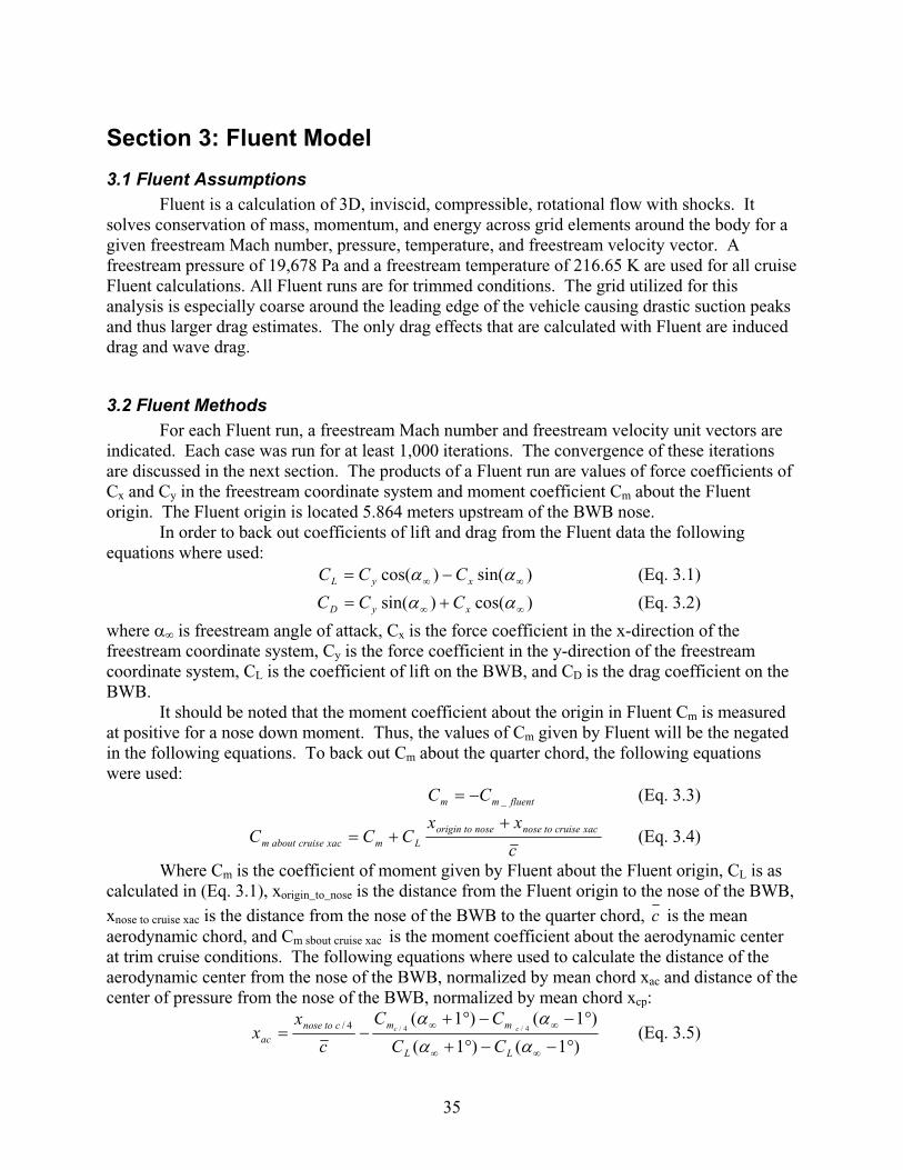
3.4 Fluent Results and AVL Comparisons for Mach 0.50 Initially Fluent cases for a freestream Mach number of 0.50 and angles-of-attack of 0, 1,

2, and 3 degrees where run and compared with the same cases run in AVL. This was done to verify that the Fluent results for the coarse BWB mesh were relatively accurate at low Mach numbers since as the drag measured at higher Mach numbers would be greater due to the coarseness of the mesh.

Figures 3.3 and 3.4 are plots of CL versus angle-of-attack and drag polar for Fluent and AVL. The values of CL versus for Fluent and AVL in figure 3.3 are only about a 0.01 difference.

37

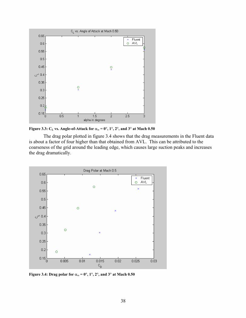
Figure 3.3: CL vs. Angle-of-Attack for = 0 , 1 , 2 , and 3 at Mach 0.50

The drag polar plotted in figure 3.4 shows that the drag measurements in the Fluent data is about a factor of four higher than that obtained from AVL. This can be attributed to the coarseness of the grid around the leading edge, which causes large suction peaks and increases the drag dramatically.

Figure 3.4: Drag polar for = 0 , 1 , 2 , and 3 at Mach 0.50

38

3.5 Fluent Results and AVL Comparisons for Cruise at Mach 0.85The main differences between AVL and Fluent is that AVL is irrotational, subsonic

incompressible, and assumes small disturbances. AVL is a vortex panel model. The figures below are results from Fluent runs compared with AVL results for cruise conditions at a Mach number of 0.85 and for angles of attack varying from -1 to 5 degrees.

Figure 3.5 shows lift versus angle of attack for both Fluent and AVL. Only smallnumbers of angle-of-attack can be compared again due to the course grid used in Fluent. At the cruise angle-of-attack of 1.656 , the required CL of 0.503 is generated. Note the large difference in CL for an angle-of-attack of 5 degrees.

Figure 3.5: Lift vs. for varying from -1 to 5 at Mach 0.85

Figure 3.6 is plot of drag polar computed in both Fluent and AVL. Fluent calculates a higher drag than AVL. At a transonic Mach number of 0.85, there is a significant influence of wave drag in the Fluent result that is not seen in the AVL computation. Note that the drag in this plot does not include the skin friction drag correction. Because the correction is the same linear contribution for both AVL and Fluent, it would not affect the relationship between the two results.

39

Figure 3.6: Drag polar for varying from -1 to 5 at Mach 0.85

Figure 3.7 is a plot of moment coefficient about the aerodynamic center location at cruise angle of attack versus lift coefficient. Values of Cm about the cruise aerodynamic center are relatively a factor of two different between AVL and Fluent. This variation in values of momentcoefficients can only be attributed to the large difference in drag between AVL and Fluent. For this cruise Mach number, there is a noticeable amount of wave drag predicted by Fluent that cannot be predicted by AVL. It increase in drag noticeably effects the moment on the vehicle.

Figure 3.7: Moment about xac at cruise vs. Lift for varying from -1 to 5 at Mach 0.85

40

Figure 3.8 is a plot of distance of the aerodynamic center and center of pressure from the nose of the BWB normalized by mean chord length. Notice that for the larger coefficients of lift, AVL and Fluent data are quite similar especially for xcp. The Fluent data has a very large relative xcp and xac values for low CL.

Figure 3.8: Distances of aerodynamic center and center of pressure from the nose of the BWB normalized by mean chord length vs. CL for varying from -1 to 5 at Mach 0.85

3.6 Static Stability The results from the Fluent calculations for distance of the aerodynamic center and center

of pressure from the nose of the BWB normalized by mean chord length that can be seen on figure 3.8 indicate that the center of pressure distance from the BWB nose is greater than the aerodynamic center distance from the BWB nose. The values of xac – xcp = { -3.0846 , -0.2876, -0.1039, 0.0161, -0.0220, -0.0499} for corresponding CL = {0.0204, 0.2128, 0.4090, 0.6227, 0.8428, 1.1788}. Thus, the Fluent results indicate the BWB is generally unstable at cruise conditions.

3.7 Fluent Results and AVL Comparisons for Cruise Angle-of-Attack at Varying Mach Number

The cruise angle-of-attack was calculated to be 1.656 . Figure 3-9 is a plot of CD

(without the skin friction correction) versus Mach numbers of 0.20, 0.30, 0.40, 0.50, 0.60, 0.70, 0.80, 0.90, 0.95, and 0.99. Note the large difference between the AVL and Fluent drag results around the transonic regions. This can be attributed to the fact that Fluent includes wave drag and AVL does not.

41

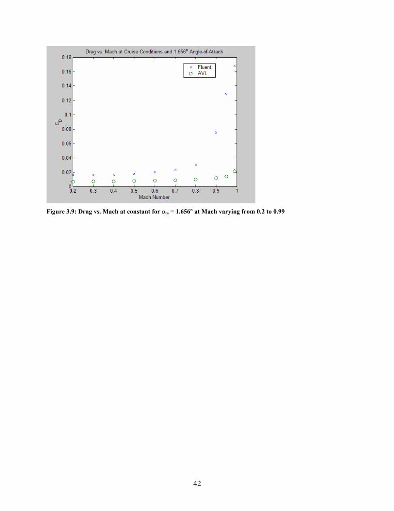
Figure 3.9: Drag vs. Mach at constant for = 1.656 at Mach varying from 0.2 to 0.99

42

Interim ConclusionIn this experiment, it was shown that the current configuration of the Blended Wing Body

design can be trimmed using flaps to meet the requirements of the approach conditions, however it cannot meet the requirements of the designated cruise conditions. All requirements can be metfor both conditions except for margin of static stability. This is the constraining parameter forthese requirements.

On approach, the BWB flies at a slower speed and higher angle of attack. This allows for the use of flaps, which AVL data shows increases stability. After some manipulation of flapsand increasing angle of attack to compensate, a satisfactory configuration was found. For this flap and alpha configuration, AVL data shows that the aircraft is stable and that the margin of stability is higher than 5%. This configuration meets the requirements for approach conditions.No redesign is required.

However, at cruise conditions, flaps would be impractical, as the body must be as streamlined as possible at high speeds. In a no-flaps configuration, at an angle of attack necessary to maintain straight and level flight at Mach .85 (cruising speed,) AVL simulationsshow a negative moment about the quarter chord. Therefore the aircraft is unstable at these conditions. This could possibly be corrected with automatic feedback control systems, however there are certain drawbacks to these systems. In an unstable aircraft, even the best feedback system will still cause an extremely bumpy ride. In order to obtain static stability at cruiseconditions, the actual shape of the aircraft must be altered.

The current configuration of the BWB cannot meet all of the requirements of this project.The body shape must be redesigned in order to meet the stability requirement.

43

Section 4: Redesign Strategy

The approach to redesign consisted of a series of sensitivity testing of different designs to find which strategy would best meet the redesign needs. In testing, only one geometriccomponent was changed in order to test the sensitivity of the component to changes in flight characteristics such as lift distribution and stability. The geometric components tested where sweep, geometric twist, and reflex. These parameters where chosen because they are commonfeatures varied on tailless aircraft to improve stability1. These sensitivity tests where analyzedwith AVL to choose a parameter for that would be used for the design iteration. These preliminary sensitivity cases are as follows:

10% increase in geometric twist10% decrease in geometric twist10% increase in sweep angle 10% decrease in sweep angle 10 increase in reflex at 70% chord The geometric twist variations are equivalent to a 10% change in the magnitude of the

local angles of attack. Thus if the local angle of attack is 1 a 10% increase would result in a local angle of attack of 1.1 . Zero degree local angles of attack remain the same. The sweep was changed by moving the airfoil sections relative to the center sections to increase and decrease the angles of sweep. The reflex was changed by using XFOIL to turn the trialing 30%of each of the fifteen airfoil sections into flaps that were deflected by the specified amounts. The reason that the reflex was added at 70% chord was due to the notice of convention for the Northrop YB-491.

After the results of these sensitivity cases where analyzed, two more cases with the chosen design iteration parameter where analyzed with AVL and with Fluent. One of the twocases where chosen, and a full analysis was done for the chosen design iteration. These two iteration parameters where as follows:

3 increase in reflex at 70% chord 4 increase in reflex at 70% chord

The following sections describe the AVL analysis for the sensitivity tests, the Fluent analysis forthe sensitivity tests, the results of the sensitivity tests, and rationale for design decisions.

4.1 AVL Redesign Methods

The various ideas for the redesigned BWB were tested through the examination ofapproach lift distributions and specific flight conditions at approach and cruise. The sectional lift distribution of the BWB at approach conditions, with no flaps deflected was examined first. Lift distributions of new designs were compared with that of the baseline BWB. It was decided thatthe new BWB design must have a lift distribution similar to, or with values less than the baseline BWB. This redesign decision was made due to the fact that the baseline design required large flap deflections on approach in order for the sectional coefficient of lift to stay below the

1 Applied Aerodynamics, “Tailless Aircraft”,<http://www.desktopaero.com/appliedaero/>, Version 4.1, DesktopAerodynamic Inc., November 13, 2003.

44

required value of 1.6 at all points on the plane. Although it was agreed that flap deflection at approach was necessary in order for stability, it was decided that it was more favorable to choose a new design that would require the same or less flap deflection on approach.

Static stability was the main component considered in our redesign and sensitivitytesting. Specifically, the static stability margin was examined for three distinct flight conditions-approach at stall, approach at trim, and cruise at trim. For the approach conditions, flaps were not deflected. The stall and trim flight conditions were determined by specific coefficient of lift values. The approach at stall coefficient of lift was found from given flight requirements, while the approach at trim and cruise at trim coefficients were found by using the equation

SV

WCL 2

2

and by assuming that lift is equal to weight at trim. Table 4.1 gives the flight conditions for the three points tested in order to determine the static stability margin.

Flight Condition Approach at Stall Approach at Trim Cruise at Trim Mach Number 0.179 0.2328 0.85

Coefficient of Lift 1.82911 1.085 0.503

Table 4.1: Flight conditions tested in sensitivity analysis

It was decided that the most important requirement in the sensitivity testing was that at the flight condition of cruise at trim, the BWB redesign be statically stable with a margin of at least 5%. This requirement was chosen as being key in the redesign because approach conditions stability and coefficient of lift distribution could be improved through the use of flaps. Flaps are not used at cruise conditions, and thus the BWB required redesign that made it automaticallystable at cruise.

4.2 Fluent Redesign Methods

The two design iteration parameter of 3 increase in reflex at 70% chord and 4 increasein reflex at 70% chord were analyzed in Fluent as well at AVL. This Fluent analysis was done solely to verify static stability predictions at cruise conditions found in the AVL analysis. This analysis in Fluent was necessary before a final design iteration geometry was chosen since the wave drag not calculated by AVL could change stability determined by Fluent. This consisted ofanalysis of redesign geometry at a cruise Mach number of 0.85 and angles of attack of -1 , 0 ,1 , 2 , and 3 . For these angles of attack CL and stability margin where analyzed.

4.3 Sensitivity Tests Results

Only cruise stability margin at trim conditions compared for each design variationbecause it was determined from our baseline geometry tests that stability could be obtained at

45

approach using flap deflection. The results of AVL analysis of the cruise stability margin at trimconditions are shown in Table 4.2.

Table 4.2: Stability margins for sensitivity testing geometry variations

Design Variation Stability Margin (%)10% increase in geometric twist -2110% decrease in geometric twist -26

10% increase in sweep angle -20.9410% decrease in sweep angle -25.72

10 increase in reflex at 70% chord 106.183

4.4 Final Design Decisions

The results of the sensitivity testing indicate that reflex was a highly influential parameterto control stability. Because the stability for a 10 reflex was much greater than expected, the relationship between static margin and reflex angle where scaled linearly and it was decided that either a 3 or 4 reflex would give satisfactory results.

AVL indicated a 16.037% and 29.288% stability margin for the 3 or 4 reflexrespectively. Figure 4.3 indicates the Fluent CL versus angle-of-attack. This plot was included to indicate approximately what angle of attack zero lift occurs.

Figure 4.3: CL vs. for varying from -1 to 3 at Mach 0.85

46

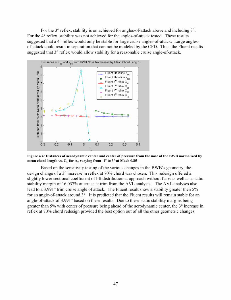
For the 3 reflex, stability is on achieved for angles-of-attack above and including 3 .For the 4 reflex, stability was not achieved for the angles-of-attack tested. These resultssuggested that a 4 reflex would only be stable for large cruise angles-of-attack. Large angles-of-attack could result in separation that can not be modeled by the CFD. Thus, the Fluent results suggested that 3 reflex would allow stability for a reasonable cruise angle-of-attack.

Figure 4.4: Distances of aerodynamic center and center of pressure from the nose of the BWB normalized by mean chord length vs. CL for varying from -1 to 3 at Mach 0.85

Based on the sensitivity testing of the various changes in the BWB’s geometry, the design change of a 3 increase in reflex at 70% chord was chosen. This redesign offered a slightly lower sectional coefficient of lift distribution at approach without flaps as well as a static stability margin of 16.037% at cruise at trim from the AVL analysis. The AVL analyses also lead to a 3.991 trim cruise angle of attack. The Fluent result show a stability greater then 5% for an angle-of-attack around 3 . It is predicted that the Fluent results will remain stable for an angle-of-attack of 3.991 based on these results. Due to these static stability margins being greater than 5% with center of pressure being ahead of the aerodynamic center, the 3 increase in reflex at 70% chord redesign provided the best option out of all the other geometric changes.

47

Section 5: Redesign Analysis Using AVL

5.1 Approach Conditions with Flaps

5.1.1 Flap Correlation Between BWB and AVL for RedesignIn the redesigned BWB, it was decided to keep the flap correlations between the BWB

and AVL the same as in the baseline design. This decision was made with the motivation of keeping the redesign as simple as possible, along with the consideration that changing flap sizes, as signified by changing the BWB and AVL correlation, would affect other considerations of the BWB design, such as structural strength or manufacturing ability. Thus, the flap correlation between the BWB and AVL in the redesign is the same as in the baseline, and is given in Table 2.1 in section 2.

Although the flap correlation remained the same in the redesigned BWB, flap settings were changed in order to accommodate for the slightly changed sectional lift distribution. As in the baseline design, the sectional lift distribution on approach conditions at stall had to be below 1.6 at all points on the wing. Thus, it was necessary to deflect flaps so as to lower the sectional coefficient of lift over the entire BWB body to within specifications. The stall conditions used were and M=.179, as calculated in section 2. Figure 5.1 gives the sectional

coefficient of lift and span loading at stall conditions on approach with no flap deflection.

829.1stallLC

Figure 5.1: Redesign sectional coefficient of lift at approach stall conditions with no flap deflection

48

Based on the examination of this distribution, and on its similarity to the baseline coefficient of lift distribution before flaps, as shown by figure 2.1 in section 2, the approach flap settings obtained for the redesigned BWB were configured as described in table 5.1.

BWB Flap # (As measured from center outward toward winglet)

Angle of Flap Deflection(In Degrees)

1 -62 03 -234 -195 -96 0

Table 5.1: Flap settings for Redesigned BWB at approach conditions

5.1.2 Trim and Stall Conditions for Redesign The coefficient of lift and Mach number for both trim and stall conditions were specified

by approach requirements. The lift coefficients were calculated using equation 2.1 as described in section 2 and are the same as the baseline lift coefficients for trim and approach. However, due to geometry changes, the angles of attack of the baseline BWB at these flight points are different from that of the redesign. The redesigned BWB’s angles of attack at trim and stall on approach were found by entering the lift coefficient and mach number for the specific flight point and then backing out the angle of attack from the output.

At stall, with a coefficient of lift of 829.1stallLC and M=.179, the redesign’s angle of

attack is =20.63 degrees. At trim, with a coefficient of lift of 085.1stallLC and M=.233, the

redesign’s angle of attack is =14 degrees.

5.1.3 Coefficient of Lift Comparison Figure 5.2 shows the coefficient of lift versus angle of attack for approach conditions

with flaps deflected for both the baseline and redesigned BWB. The stall and trim conditions of the redesigned BWB are also noted in the figure.

49

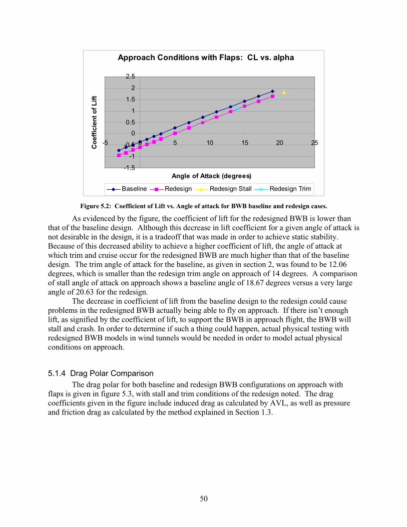
Approach Conditions with Flaps: CL vs. alpha

-1.5

-1

-0.5

0

0.5

1

1.5

2

2.5

-5 0 5 10 15 20 25

Angle of Attack (degrees)

Co

effi

cien

t o

f L

ift

Baseline Redesign Redesign Stall Redesign Trim

Figure 5.2: Coefficient of Lift vs. Angle of attack for BWB baseline and redesign cases.

As evidenced by the figure, the coefficient of lift for the redesigned BWB is lower than that of the baseline design. Although this decrease in lift coefficient for a given angle of attack is not desirable in the design, it is a tradeoff that was made in order to achieve static stability.Because of this decreased ability to achieve a higher coefficient of lift, the angle of attack at which trim and cruise occur for the redesigned BWB are much higher than that of the baseline design. The trim angle of attack for the baseline, as given in section 2, was found to be 12.06 degrees, which is smaller than the redesign trim angle on approach of 14 degrees. A comparisonof stall angle of attack on approach shows a baseline angle of 18.67 degrees versus a very large angle of 20.63 for the redesign.

The decrease in coefficient of lift from the baseline design to the redesign could cause problems in the redesigned BWB actually being able to fly on approach. If there isn’t enough lift, as signified by the coefficient of lift, to support the BWB in approach flight, the BWB willstall and crash. In order to determine if such a thing could happen, actual physical testing with redesigned BWB models in wind tunnels would be needed in order to model actual physical conditions on approach.

5.1.4 Drag Polar Comparison The drag polar for both baseline and redesign BWB configurations on approach with

flaps is given in figure 5.3, with stall and trim conditions of the redesign noted. The drag coefficients given in the figure include induced drag as calculated by AVL, as well as pressure and friction drag as calculated by the method explained in Section 1.3.

50

Approach Conditions with Flaps: Drag Polar

-1.5

-1

-0.5

0

0.5

1

1.5

2

2.5

0 0.05 0.1 0.15 0.2 0.25

Coefficient of Drag (total)

Co

effi

cien

t o

f L

ift

Baseline Redesign Redesign Stall Redesign Trim

Figure 5.3: Drag Polar for Baseline and Redesigned BWB on Approach with Flaps

The drag coefficient of the redesign is in general slightly less than that of the baseline forany given coefficient of lift. This is most likely in part due to the redesigned BWB having less lift for any given angle of attack than the baseline. Such a difference would cause a decrease in the induced drag of the redesigned BWB from the baseline. Induced drag is dependent on the coefficient of lift, and thus for lower coefficients of lift, the induced drag is lower. Having a lower drag coefficient for the redesigned BWB is a plus, although in this case it signifies the lower lift values achieved by the BWB in approach flight.

5.1.5 Moment Coefficient About Aerodynamic Center Comparison The moment coefficient, as measured around the aerodynamic center, versus the

coefficient of lift is shown in figure 5.4. These values are for the BWB baseline and redesign on approach with flaps deflected. Stall and trim conditions of the redesign are also noted for reference.

51

Approach Conditions with Flaps: Mac vs. CL

0

0.2

0.4

0.6

0.8

1

1.2

1.4

-1.5 -1 -0.5 0 0.5 1 1.5 2 2.5

Coefficient of Lift

Mo

men

t C

oef

fici

ent

abo

ut

Xac

Baseline Redesign Redesign Stall Redesign Trim

Figure 5.4: Moment about aerodynamic center vs. coefficient of lift for approach with flaps.

The redesigned BWB has a linear relationship between moment coefficient and coefficient of lift, although this relationship is not constant, as would be expected. The definition of the aerodynamic center is the location at which the moment is constant with respect to changes in angle of attack. Since angle of attack and coefficient of lift have a linear relationship, as seen by figure 5.2 in this section, the moment about the aerodynamic center should also be constant for changes in lift coefficient. The baseline BWB appears to mirror that relationship with only small variances.

The significance of these results is that for the redesigned BWB, a change in coefficient of lift (and thus angle of attack) will increase the moment about the aerodynamic center, causing the nose of the plane to pitch up. This could cause problems in dynamic stability and could also affect static stability by causing the true aerodynamic center (as given by the definition) to movearound with increase in alpha, thus affecting the static stability margin as compared with the center of pressure.

5.1.6 Aerodynamic Center, Center of Pressure, and Static Stability for Redesign Figure 5.5 shows the distance of the aerodynamic center and the center of pressure from

the nose of the BWB as a function of coefficient of lift. The trim flight point’s aerodynamiccenter and center of pressure are also noted in the figure. The distance values have been normalized by the mean aerodynamic chord length of c = 9.3661 m. The figure does not include a large dip in center of pressure that occurs at LC 0 with an =-42. The figure has been

made to highlight usual flight conditions so as to properly examine the static stability of the redesigned BWB.

cpx

52

Redesign at Approach Conditions, With Flaps: Xac and Xcp

-2

-1

0

1

2

3

4

5

6

-1.5 -1 -0.5 0 0.5 1 1.5 2

Coefficient of Lift (Cl)

Dis

tan

ce f

rom

No

se (

m)

Aerodynamic Center Center of Pressure Trim Xac Trim Xcp

Figure 5.5: Aerodynamic center and center of pressure vs. lift coefficient for approach conditions of redesigned BWB with flaps deflected.

As explained in section 2, static stability requires the center of pressure to be in front ofthe aerodynamic center by a certain distance. This distance is a specification of design, and for the BWB is given in the form of a margin of 5%. This means that the aerodynamic center is a distance of at least 5% of the mean aerodynamic chord away from the center of gravity. As our values are non-dimensionalized by the mean aerodynamic chord, the above figure shows the redesigned BWB to be stable if the aerodynamic center and center of pressure are at least a distance of .05 apart.

As seen by figure 5.5, the redesigned BWB is quite stable for a wide range of lift coefficients. It becomes unstable for negative lift coefficients around LC -0.2. This is a highlyfavorable outcome, since the main goal in redesign was to make sure the BWB remainedstatically stable. However, due to the amount of lift generated per angle of attack, the corresponding angle of attack with LC -0.2 is around 3 degrees. Although this is a usual flight angle for an aircraft, it isn’t likely that on approach a plane would fly with this low of an angle of attack.

At trimmed approach with flaps, the location of the redesigned BWB’s non-dimensionalized center of pressure is at cpx 2.726. The aerodynamic center’s location is at

3.056, thus giving a static stability margin of .330, or 33%. acx

At stalled approach with flaps, the location of the center of pressure for the redesigned BWB is at 2.825, with an aerodynamic center location of cpx acx 2.888. These values yield a

static stability margin of 6.33%. The fact that the redesigned BWB is statically stable even at stall is favorable to the design.

The redesign, as compared with the baseline BWB, is more statically stable. Figure 5.6 shows the difference between and versus lift coefficient for the baseline and redesign acx cpx

53

configurations of the BWB. This difference gives the static stability margin as represented in decimal form. Positive values indicate stability, while negative values indicate instability. The trim conditions for both the baseline and redesign are also noted in the figure.

Static Stability Margin vs. Lift Coefficient

-2

-1.5

-1

-0.5

0

0.5

1

1.5

2

-1.5 -1 -0.5 0 0.5 1 1.5 2 2.5

Lift Coefficient

Sta

tic

Sta

bili

ty M

arg

in

Baseline Redesign Baseline Trim Redesign Trim

Figure 5.6: Static Stability Margin vs. Lift Coefficient comparison for baseline and redesigned BWB.

Figure 5.6 shows that the redesigned BWB is in general more stable than the baseline.Especially notable is the stability of the redesign near LC 0, which is a complete change fromthe baseline design. Although both configurations are unstable for lift coefficients less than 0.5, the redesign is less stable than the baseline.

In general, these results indicate that the main goal of the redesign, to increase staticstability, has been achieved. There are more values of for which the BWB is stable in the redesign than in the baseline. In addition, as seen by the figure, static stability at trim, an important flight point, has been increased through the redesign, from 23.6 % margin to 33% margin. Although not noted on the figure, the stability margin at stall has also been increased due to redesign. The baseline BWB was not stable and had a margin of 2.0%. However, through redesign, that margin has increased to 6.3%, thus showing static stability as specified by the design constraints.

LC

5.1.7 Lift Distribution and Span Loading for Redesign

5.1.7.1 Approach at Trim ConditionsFigure 5.7 shows the span loading and sectional coefficient of lift distribution for the

BWB at trimmed approach conditions on half of the body. It may be assumed that this distribution is symmetrical for the whole body. This plot is similar in notation to those provided earlier.

54

Figure 5.7: Span loading and sectional coefficient of lift vs. span length for approach conditions of redesignedBWB with flaps deflected at trim.

As compared with these quantities at baseline, as seen in figure 2.6 of section 2, the distributions are almost exactly similar. The only barely imperceptible difference can be seen near the trailing edge, where the sectional coefficient of lift and span loading values of the redesign are only slightly higher than that of the baseline. This change is due to the slight difference in flap settings between the baseline and redesign approach configurations. As withthe baseline, the redesign’s large peak in sectional lift coefficient near the edge of the airfoil is due to the winglet. The span loading, similar to the baseline design, is greatest near the root of the wing and decreases significantly around the half point of the wing. The lift to drag ratio at trimmed approach conditions with flaps can be calculated by finding the ratio of the coefficient of lift over the drag coefficient. In section 2, the ratio of the baseline design was found to be 12.463. The redesign’s lift to drag ratio is

D

L=13.045

55

56

A larger lift to drag ratio is more favor use it represents more lift with less dragenalty, a major consideration in flight. From the information about the comparison in lift

does

The span loading and sectional coefficient of lift distribution for the BWB at stalled5.8.

Fi ithflaps

em that they are almost exactly similar. One minor goal of the redesign ions similar to the baseline, so as to not have to redesign or

able, becapcoefficient between the redesign and the baseline, along with this lift to drag ratio, it can be seen that although the redesign does have less lift for a given angle of attack than the baseline, itnot suffer in drag penalties. The fact that the lift to drag ratio is greater for the redesign is positive and makes up for some of its shortcomings ability to generate lift.

5.1.7.2 Approach at Stall Conditions

approach conditions is shown in figure

gure 5.8: Span loading and sectional coefficient of lift vs. span length for approach conditions of BWB w deflected at stall.

Again, when this figure is compared with the distributions of the baseline in figure 2.7 of ection 2, it can be ses

was to keep sectional lift distribut

reconfigure flaps. It was decided that such a goal would keep the BWB redesign simple and thuseasier to make stable, as it was found that the baseline BWB on approach was statically stable.Thus, flap settings for the redesign on approach were kept similar, causing sectional coefficienof lift and span loading distributions to remain the same for approach at trim and stall.

The lift to drag ratio for stall of the redesign, on approach, was found to be

t

D=10.302

L

as compared with that of the baseline, calculated in section 2, of 9.745. Again, this signifies a favorable change, even though through other risons between the baseline and redesign show a decrease in the redesign’s lift for a given angle of attack. As was true with the baseline

ll

ndition Analysis with AVLWith the redesign, at cruise (Mach number 0.85) the BWB is considered trimmed at an

angle of

lift compa

configuration, the lift to drag ratio is smaller at stall than at trim because more drag exists at staon the aircraft.

5.2 Cruise Co

=3.99 degrees. At these conditions, the aerodynamic center is locatedure is x =3.062, which are non-acx =3.222 from the nose, and the center of press cp

dimensionalized values as normalized by the mean aerodynamic chord ( c = 9.3661 m). At thesconditions, the center of pressure is located in front of the aerodynamic center, thus

esignifying a

sta irement for

The redesigned BWB satisfies the required approach conditions specifications and constraints and is also stable at cruise. The stability margin has been increased, although this

a design trade off of a decreased coefficient of lift for a given angle of nough

edn

ble arrangement. The static stability margin is 16%, satisfying the stability requthe BWB. As compared with the baseline redesign, in which the BWB at cruise was very unstable (margin -23.6%), this is very much an improvement.

5.3 Conclusion

increase has causedattack. This decrease in lift could cause problems in real physical flight by not providing eforce to keep the BWB aloft. Although this design trade off exists, drag has also been decreasthrough the redesign, with lift to drag ratios increasing, showing that although lift generatiocapabilities of the redesign have been lessened, there is no significant increase in drag penalty.Large flap deflections are still needed to fulfill approach requirements, which could cause problems with local flow separation and stability. However, the redesign’s positive changes from the baseline appear to outweigh the negative changes. Further physical testing would be needed to decide if the redesign would fly well in real flight conditions.

57

Section 6: Fluent Model Analysis of Redesign

6.1 Fluent Analysis Overview Fluent is a calculation of 3D, inviscid, compressible, rotational flow with shocks. It

solves conservation of mass, momentum, and energy across grid elements around the body for a given freestream Mach number, pressure, temperature, and freestream velocity vector. A freestream pressure of 19,678 Pa and a freestream temperature of 216.65 K are used for all cruise Fluent calculations. All Fluent runs are for trimmed conditions. The grid utilized for the redesign analysis is much coarser than the grid used to analyze the baseline geometry in the section above. It is especially coarse around the leading edge of the vehicle causing drastic suction peaks and thus larger drag estimates. Thus, drag calculated by Fluent is expected to be relatively large due to the coarseness of the grid. The only drag effects that are calculated with Fluent are induced drag and wave drag. All Fluent runs where allowed to run to convergence to avoid error.

6.2 Fluent Results and AVL Comparisons for Redesign BWB Geometry Cruise at Mach 0.85

The figures below are results from Fluent runs compared with AVL results for a 3 reflex at 70% chord for cruise conditions at a Mach number of 0.85 and for angles of attack varying from -1 to 4 degrees. All plots have drag values not corrected for pressure and friction drag since these corrections would add the same values to both the Fluent and AVL results and makeno change in the comparison of the two CFD methods.

Figure 6.1 shows lift versus angle of attack for both Fluent and AVL. Only smallnumbers of angle-of-attack can be compared again due to the course grid used in Fluent. Note the large difference in CL for an angle-of-attack of above 0 . This can be attributed to the coarseness of the Fluent mesh in addition to the wave drag calculated by Fluent not calculated by AVL. For the cruise trim angle-of-attack of 3.991 , Fluent predicts that the required CL of 0.503 is not obtained. This is unfortunate.

58

Figure 6.1: Lift vs. for varying from -1 to 4 at Mach 0.85

Figure 6.2 is plot of drag polar computed in both Fluent and AVL. Fluent calculates a higher drag than AVL. At a transonic Mach number of 0.85, there is a significant influence of wave drag in the Fluent result that is not seen in the AVL computation. Note that the drag in this plot does not include the skin friction drag correction. The drag calculated by Fluent is approximately a factor of seven higher than the drag calculated by AVL. This large drag difference can be contributed mainly to the coarseness of the redesign Fluent grid.

Figure 6.2: Drag polar for varying from -1 to 4 at Mach 0.85

59

Figure 6.3 is a plot of moment coefficient about the cruise trim aerodynamic center location versus lift coefficient for varying angles of attack. There is a large inconsistencybetween Fluent and AVL for Cm versus CL. It can be noted from figure 6.4 below that Fluent and AVL xac values are pretty constant and approximately the same values. The xcp values in figure 6.4 between Fluent and AVL are more different. This varied relative motion of xcp for thedifferent CFD calculation methods offers some explanation of the plot in figure 6.3. Otherwise, the difference between Cm versus CL for Fluent and AVL can not be explained. The Fluent results make more sense based on the definition of moment about aerodynamic center.

Figure 6.3: Moment about xac at cruise vs. lift for varying from -1 to 4 at Mach 0.85

60

Figure 6.4: Distances of aerodynamic center and center of pressure from the nose of the BWB normalized by mean chord length vs. CL for varying from -1 to 4 at Mach 0.85

6.3 Static Stability The results from the Fluent calculations for distance of the aerodynamic center and center

of pressure from the nose of the BWB normalized by mean chord length that can be seen on figure 6.4 indicate that the center of pressure distance from the BWB nose is greater than the aerodynamic center distance from the BWB nose for CL values less than 0 and the center of pressure distance from the BWB nose is less than the aerodynamic center distance from the BWB nose for CL values greater than about 0. The values of xac – xcp = {-0.4940, -0.7278, -1.3339, -5.3050, 2.7662, 1.1036} for corresponding CL = {-0.2058, -0.1448, -0.0826, -0.0210, 0.0403, 0.1006}. Thus, the Fluent results indicate the BWB is stable at cruise conditions. Yay!

6.4 Fluent Results and AVL Comparisons for Cruise Angle-of-Attack at Varying Mach Number

The cruise angle-of-attack was calculated to be 3.991 . Figure 6.5 is a plot of CD

(without the skin friction correction) versus Mach numbers of 0.20, 0.30, 0.40, 0.50, 0.60, 0.70, 0.80, 0.90, 0.95, and 0.99. Note the large difference between the AVL and Fluent drag results around the transonic regions. This can be attributed to the fact that Fluent includes wave drag and AVL does not.

61

Figure 6.5: Drag vs. Mach at constant for = 3.991 at Mach varying from 0.2 to 0.99

62

Final Conclusion In the Interim Report, it was determined that the baseline geometry of the Blended Wing

Body aircraft did not meet the requirements of this project. According to both AVL and Fluent simulations, the baseline geometry was not stable at cruise conditions. With significant flapdeflection, a configuration for approach conditions was found in which the aircraft was stable, however this design could not operate under cruise conditions.

The goal of the redesign phase was to change the geometry of the aircraft to increase stability at cruise conditions. After running a series of sensitivity tests using AVL, it was determined that adding a reflex to the shape of all the airfoils along the BWB could cause a significant improvement in the stability of the aircraft. New BWB models were then createdwith reflexes of 1, 2, 3, 4 and 10 degrees. AVL simulations were run on each of these airfoils and it was discovered that a reflex of 3 degrees caused the aircraft to be statically stable with a reasonable margin of stability. This geometry was selected as the final redesigned geometry.

To support the AVL simulations, an equivalent geometry was tested using Fluent. The results corroborated the conclusion that the redesigned BWB was statically stable, but the Fluent simulation returned a much smaller CL at the angle of attack AVL determined to be necessary at cruise conditions. This data suggests that the wave effects and suction peaks that AVL cannot simulate may reduce the CL of the redesigned BWB to the point where it cannot fly.

However, the Fluent calculation of the CL may be significantly underestimated. The meshes created for testing the redesigned aircraft were particularly coarse, especially along the leading edge. This means that the Fluent flow solution may contain large suction peaks where the actual redesigned aircraft in flight would not experience them. This would cause the Fluent predicted lift to be too low and the drag to be too high.

Since such a large discrepancy was observed between the AVL and Fluent models, it can be assumed that neither model is entirely accurate. Whether the redesigned aircraft can actually generate enough lift to stay aloft at cruise conditions cannot be determined for certain by either one of these methods. More extensive wind tunnel testing at higher Mach numbers may be necessary to gain a better estimate for actual lift generated at cruise conditions.

Through Fluent and AVL simulations, it was determined that the redesigned BWBaircraft is statically stable at cruise conditions, however results differed as to whether the redesigned aircraft could generate enough lift to fly at the specified conditions. Further testing is necessary to determine lift with any certainty.

63

Appendix A: Distribution of Tasks

Interim Report

Written deliverables: Introduction: Tanya Overview of Methods Used: Brady Section 1: Wind Tunnel Model: JuliaSection 2: AVL Model: AmySection 3: Fluent Model: Tanya Interim Conclusion: Brady

Non-deliverable contributions: Wind Tunnel post processing: JuliaAVL data collection: AmyAVL spreadsheet maintenance: Brady and Amy Fluent data collection and post processing: Tanya Compiler: Brady

Final Report

Written deliverables: Corrections to Interim Report: same team member who wrote original deliverableSection 4: Redesign Strategy: Amy and TanyaSection 5: Redesign Analysis Using AVL: Amy Section 6: Redesign Analysis Using Fluent: TanyaFinal Conclusion: BradyAppendix B: Frequently Used Parameters: Julia

Non-deliverable contributions: Skin friction and Pressure Drag calculation: BradySkin friction and Pressure Drag write-up: JuliaRedesign Strategy: all team members collaborated to come up with strategy Generated Redesigned Geometry in Matlab: Tanya, with some help from JuliaSensitivity testing on AVL: AmySenitivity testing post-processing: JuliaFinal design testing on AVL: Amy and Brady Final design testing on Fluent: Tanya Spreadsheet Maintenance: Brady and Amy

64

Appendix B: Tables of Numerical Quantities

Parameter Symbol Value UnitsReference Area

refS 728.36 2m

Wetted AreawetS 1423.74 2m

Span Length b 88.09 mMean AerodynamicChord

c 9.37 m

X Location of Mean Aerodynamic Chord

cx 27.17 m

Y Location of Mean Aerodynamic Chord

cy 24.14 m

Quarter Chord Point 4/cx 29.51 m

Max Take Off Weight

MTOW 662546.75 lbs

5% Stability Margin 0.05 NA

Table B.1: BWB Dimensional Quantities

Parameter Symbol Value UnitsDynamic Pressure q 50 mph: 302.04

100 mph: 1197.24 2ms

kg

Height of Wind Tunnel H 2.134 mWidth of Wind Tunnel W 3.048 mWind Tunnel Aspect Ratio 0.7 NAEffective Span to JetWidth Ratio

k 0.5534 NA

Table B.2: Wind Tunnel Dimensional Quantities

Parameter Symbol Value50 mph | 100 mph

Reynolds Number Re 510*557.2 510*108.5Mach Number M 0.067 0.135Cylindrical Support Drag Coefficient

csDC 0.8 0.8

Balance Arm Skin Friction Coefficient

fc 0.005 0.0045

Balance Arm Drag Coefficient

baDC 0.01 0.009

Balance Support Drag Coefficient

bsDC 0.35 0.35

Table B.3: Wind Tunnel Calculated Values

65

Parameter Symbol Value UnitsFreestream Density at 39000 ft

0.31753m

kg

Speed of Sound at 39,000 ft

a 350.79

s

m

Freestream Mach cruiseM 0.85 NA

Skin Friction Drag Coefficient

fDC 0.0083034 NA

Pressure Drag Coefficient, Trim

pDC 200869.000038704.0 lC NA

Table B.4: Cruise Conditions

Parameter Symbol Value UnitsSpeed of Sound at Sea Level, STPconditions

a 331

s

m

Density of Air at Sea Level

1.253m

kg

Freestream Mach at Trim

trimM 0.2328 NA

Freestream Mach at Stall

stallM 0.179 NA

Skin Friction Drag Coefficient

fDC 0.01041 NA

Pressure Drag Coefficient

pDC 2018995.00004854.0 lC NA

Table B.5: Approach Conditions

66

Appendix C: Design Team vs. Hammock

Figure C.1: From left to right: Tanya “The Imaginary One” Cruz Garza, Julia “Paranoid” Thrower, John D.“Bring Me To The Party” Anderson, Amy “Distracted” Brzezinski, Brady “Forgetful” Young, one very

stressed out hammock

67

Appendix D: Matlab Code for Fluent Graphs (see attached sheets for code)

Figure 3.1 Fluent CL vs. Iterations plot for Mach 0.50Filename: plot_resid_cl.m

Figure 3.2 Fluent Cm vs. Iteration about the quarter chord for Mach 0.85 Filename: plot_resid_cm.m

Figure 3.3 CL vs. Angle-of-Attack for = 0 , 1 , 2 , and 3 at Mach 0.50Filename: machhalf.m

Figure 3.4 Drag polar for = 0 , 1 , 2 , and 3 at Mach 0.50Filename: machhalf.m

Figure 3.5 Lift vs. for varying from -1 to 5 at Mach 0.85 Filename: macheightyfive.m

Figure 3.6 Drag polar for varying from -1 to 5 at Mach 0.85 Filename: macheightyfive.m

Figure 3.7 Moment about xac at cruise vs. Lift for varying from -1 to 5 at Mach 0.85 Filename: macheightyfive.m

Figure 3.8 Distances of aerodynamic center and center of pressure from the nose of the BWBnormalized by mean chord length vs. CL for varying from -1 to 5 at Mach 0.85Filename: macheightyfive.m

Figure 3.9 Drag vs. Mach at constant for = 1.656 at Mach varying from 0.2 to 0.99 Filename: alphaoneptsix.m

Figure 4.3 CL vs. for varying from -1 to 3 at Mach 0.85Filename: macheightyfive_sensitivitytests.m

Figure 4.4 Distances of aerodynamic center and center of pressure from the nose of the BWBnormalized by mean chord length vs. CL for varying from -1 to 3 at Mach 0.85 Filename: macheightyfive_sensitivitytests.m

Figure 6.1 Lift vs. for varying from -1 to 4 at Mach 0.85 Filename: macheightyfive_redes.m

Figure 6.2 Drag polar for varying from -1 to 4 at Mach 0.85 Filename: macheightyfive_redes.m

Figure 6.3 Moment about xac at cruise vs. lift for varying from -1 to 4 at Mach 0.85

68

Filename: macheightyfive_redes.m

Figure 6.4 Distances of aerodynamic center and center of pressure from the nose of the BWBnormalized by mean chord length vs. CL for varying from -1 to 4 at Mach 0.85 Filename: macheightyfive_redes.m

Figure 6.5 Drag vs. Mach at constant for = 3.991 at Mach varying from 0.2 to 0.99 Filename: alphathree.m

69