VSGCP-E-91-001 C3

VIRGINIA SEA GRANTCOLLEGE PROGRAM

TEACHERS’ GUIDE FORUSING APT SATELLITE IMAGERYTO TEACH SCIENCE AND MATH

This work is the result of research sponsored in partby the National Oceanic and Atmospheric Administration,U.S. Department of CommerceSea Grant No. NA9OAA-D-SG840

Tri-Space, Inc.P.O. Box 7166

MC Lean, Virginia 22106

VSG-91-05

This work is a result of researchsponsored in part by the NationalSea Grant College Programof the National Oceanic andAtmospheric Administration,U.S. Department of Commerce,under Grant No. NA86AA-D-SG042 to the Virginia MarineScience Consortium and theVirginia Sea Grant College Pro-gram. The U.S. Government isauthorized to produce anddistribute reprints for govern-mental purposes notwithstand-Ing any copyright notation thatmay appear hereon.

TEACHERS’ GUIDE FORUSING APT SATELLITE IMAGERYTO TEACH SCIENCE AND MATH

Author: E. Ann BermanCo-author: Jim FletcherMeteorological Consultant: Hank Brandli

July 1991

Tri-Space, Inc.P.O. Box 7166MC Lean, Virginia 22106

This work is a result of research sponsoredin part by the National Oceanic and Atmospheric Administration,U.S. Department of Commerce Sea Grant No. NA90AA-D-SG840

Acknowledgements

This work could not have been undertaken without the assistance of the Virginia SpaceGrant Consortium, a coalition of five Virginia colleges and universities, NASA, stateeducational agencies, museums, private industry associations, and other institutions withdiverse education and aerospace interests. Throughout this effort the Consortium hasworked diligently on enhancing public awareness of the benefits of space related researchand in the use of satellite APT imagery to enhance science and math curricula. Theirpromotion of strong science and math programs is to essential to the success of this Guide.

I wish to extend my gratitude to Jim Fletcher, who not only contributed the Unit onAgricultural Applications, but devoted many hours to capturing the west coast images usedthroughout the Guide. His interest in the Guide and encouragement along the way wereinvaluable. I extend my thanks also to Hank Brandli who provided most of themeteorological annotation and interpretation for the images used herein. Hank alsoprovided substantial insight and guidance on the content of the meteorological units.Thanks also to my husband Jim for his patience while this book was in preparation, hissuggestions and careful editing of the document.

This work was sponsored in part by NOAA, Sea Grant, Department of Commerce, underGrant NA90AA-D-SG840. The image of twin hurricanes off the coast of the Baja Peninsulawas provided courtesy of Lockheed Missiles and Space, Austin Division. The GOES imagewas provided courtesy of Thomas Jefferson Science High School, Fairfax County, Virginia.

TABLE OF CONTENTS

Introduction

Unit 1: Remote Sensing Mechanics - Image Processing

1.1 What Is a Pixel? 1.11.2 The Value of Grey Shades 1.21.3 Intermediate Study: Understanding Histograms 1.31.4 Advanced Study: Image Enhancement/Contrast Stretching 1.41.5 Summary Discussion 1.6

Unit 2: Remote Sensing - The Electromagnetic Radiation

2.1 Waves are Patterns not Matter 2.12.2 Electromagnetic Spectrum 2.32.3 Planck’s Law - The Brightness of the Sun and Earth 2.32.4 The TIROS-N AVHRR is a Radiometer 2.42.5 Reflectance is the Key to Meteor and Band 2 Images 2.52.6 Temperature is the Key to Bands 3 and 4 2.112.7 Intermediate Study: Black Body Radiation 2.132.8 The Atmosphere’s Content 2.142.9 Advanced Study: Radiative Transfer in the Atmosphere 2.152.10 Summary Discussion 2.16

Unit 3: The State of the Atmosphere - How Clouds are Formed

3.1 Temperature and Atmospheric Circulation 3.13.2 Pressure and Atmosphere 3.13.3 Thermodynamics 3.23.4 Water Vapor 3.33.5 How Clouds Form 3.43.6 Summary Discussion 3.9

Unit 4: Cloud Types - How Do We Recognize Them

4.1 Classifying Clouds4.2 Low Clouds4.3 Middle Clouds4.4 High Clouds4.5 Summary Discussion

4.14.44.84.104.12

Unit 5: Upper Level Air Flow

5.1 Ridges and Troughs5.2 Waves5.3 The Jet Stream5.4 Summary Discussion

Unit 6: Weather Systems

6.1 Fronts 6.16.2 Severe Storms 6.66.3 Tropical Storms 6.96.4 Summary Discussion 6.15

Unit 7: Applications of Infrared Images to Oceanography

7.1 Tracking Ocean Currents 7.17.2 Ocean Fronts and Eddies 7.27.3 Locating Fish 7.37.4 Summary and Discussion 7.6

Unit 8: Applications of Visible Images to Agriculture

8.1 Timing of Tillage and Field Operations 8.18.2 Herbicide Selection and Timing of Application 8.18.3 Timing of Additional Field Operations 8.38.4 A Winter Wheat Season in the Palouse 8.38.5 Summary and Discussion 8.9

5.15.45.75.9

Appendix A: Glossary A-l

List of Images

-

Image 1.1

Image 1.2

Image 1.3

Image 2.1

Image 2.2

Image 2.3

Image 2.4

Image 2.5

Image 2.6

Image 2.7

Image 2.8

Image 2.9

Image 3.1

Image 3.2

Image 3.3

Image 3.4

Image 3.5

Image 3.6

Image 3.7

Image 3.8

Increasing grey shades improves the information displayed in an images.

A Soviet Meteor image of the Gulf Coast of the United States.

The same Meteor image stretched over a range of pixel values from 24 to 64.

Illustration of an upper level wave over the Western United States.

Stretched Meteor image of the Gulf Coast of the United States.

Visible (band 2) image of the Northeastern United States on a clear day.

Meteor visible image showing reflectance characteristics of ice, snow and water.

Meteor image showing the dendritic pattern of snow.

Meteor image showing the reflectance of sand and soils.

TIROS-N band 2 image showing the reflectance of everglades vegetation.

In thermal infrared images, warm features are black and cold objects are white.

TIROS-N infrared image of twin hurricanes off the West Coast of Mexico.

Fog in California’s San Joaquin Valley.

Fog in Western Rocky Mt. Valleys.

Clouds form due to orographic lifting over the Blue Ridge Mountains.

Cloud dissipation on the leeward side of the Sierra Nevadas.

Lifting attributed to convergence of air as it passes through the Casper Gap.

GOES infrared image showing the ITCZ and the subtropical high pressure belts.

Sea breezes.

Santa Ana winds cause upwelling cold water off the coast. Air is sinking in theclear areas.

Image 4.1 Cloud height relates to temperature on infrared images.

Image 4.2 Infrared view of low level cumuliform and stratiform clouds.

Image 4.3 FengYun infrared view of stratocumulus cloud streaks.

Image 4.4 Visible image of various cumulus and stratus clouds over the northeast.

Image 4.5 Infrared image of cumulus and stratus cloud forms.

Image 4.6 Open cell cumulus over the Pacific Ocean from NOAA 11.

Image 4.7 Band 2 view of mid level clouds.

Image 4.8 Infrared view of mid level clouds.

Image 4.9 Visible image of cumulonimbus storm clouds.

Image 4.10 Infrared image of cumulonimbus clouds with coldest cloud tops blackened.

Image 4.11 Band 2 image of cirrus and cirrostratus clouds.

Image 4.12 Infrared image of cirrus and cirrostratus clouds.

Image 5.1 Troughline over the Pacific Ocean seen in a band 2 image.

Image 5.2 Troughline over the Atlantic Ocean seen in an infrared image.

Image 5.3 Ridgelines are marked by upper level cirrus clouds.

Image 5.4 Zonal Flow over the eastern U.S. marked by cirrus clouds in

Image 5.5 Zonal Flow over the western U.S. marked by the jet stream.

Image 5.6 Jet stream cirrus clouds are grey in a visible image.

Image 5.7 Jet stream cirrus clouds are white in an infrared image.

Image 6.1 A cold front off the east coast of the United States.

Image 6.2 An occluded front.

Image 6.3 An occluded front with rain and snow forecast.

Image 6.4 A rope cloud marks the edge of the frontal system.

the jet stream.

Image 6.5 Gust fronts form in advance of thunderstorms.

Image 6.6 Squall lines form in advance of fronts.

Image 6.7 Visible image of storm system.

Image 6.8 Infrared image of storm system.

Image 6.9 Cold front with thunderstorm activity.

Image 6.10 Tropical storm Lili at about 3 p.m. on October 11, 1991.

Image 6.11 Infrared view of tropical storm Lili.

Image 6.12 Tropical storm Lili late afternoon on October 12, 1991.

Image 6.13 By morning of October 13, 1991 tropical storm Lili has burned itself out.

Image 6.14 Hurricane Bertha on 31 July, 1991.

Image 6.15 Close up view of hurricane Bertha in the visible band.

Image 7.1 Warm core eddies and cold core rings developing at the Gulf Stream boundary.

Image 7.2 Three warm core eddies along the continental shelf.

Image 8.1 Infrared image of a storm affecting herbicide application.

Image 8.2 The Palouse wheat growing region of eastern Washington.

Image 8.3 Rain after planting starts the crop off right.

Image 8.4 November’s first snowfall is disappointing at lower elevations.

Image 8.5 December’s frigid air and high winds cause widespread damage.

Introduction

Overview:

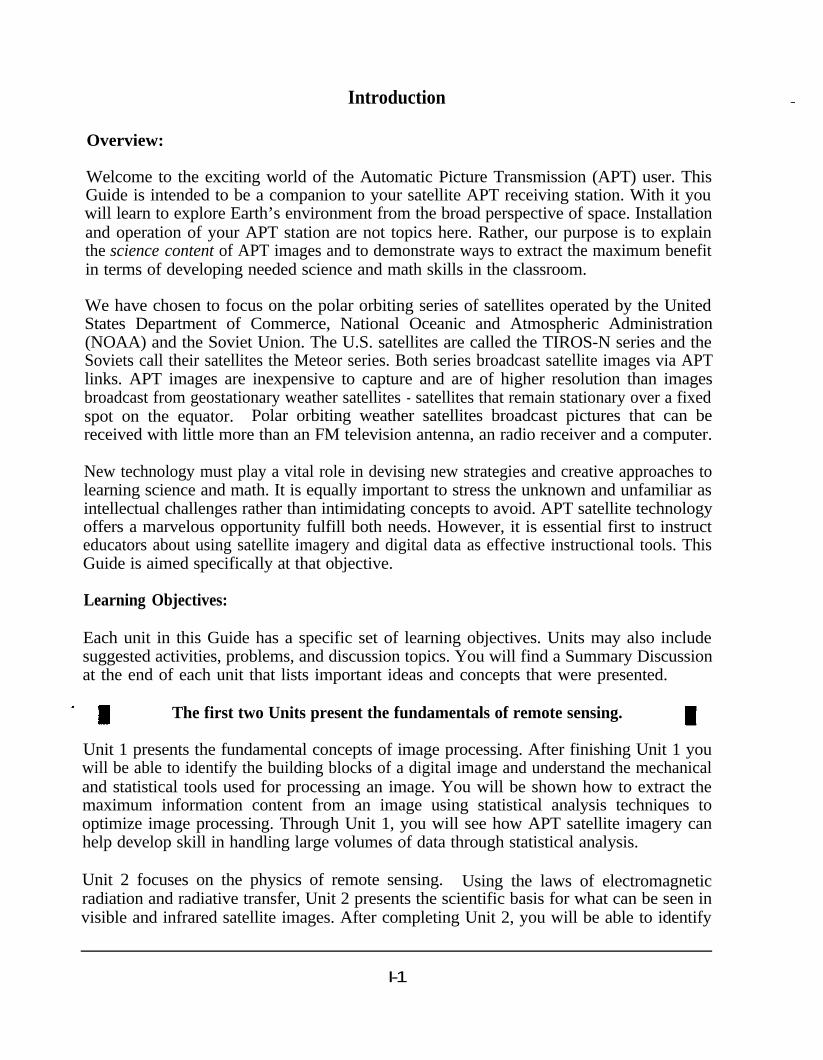
Welcome to the exciting world of the Automatic Picture Transmission (APT) user. ThisGuide is intended to be a companion to your satellite APT receiving station. With it youwill learn to explore Earth’s environment from the broad perspective of space. Installationand operation of your APT station are not topics here. Rather, our purpose is to explainthe science content of APT images and to demonstrate ways to extract the maximum benefitin terms of developing needed science and math skills in the classroom.

We have chosen to focus on the polar orbiting series of satellites operated by the UnitedStates Department of Commerce, National Oceanic and Atmospheric Administration(NOAA) and the Soviet Union. The U.S. satellites are called the TIROS-N series and theSoviets call their satellites the Meteor series. Both series broadcast satellite images via APTlinks. APT images are inexpensive to capture and are of higher resolution than imagesbroadcast from geostationary weather satellites - satellites that remain stationary over a fixedspot on the equator. Polar orbiting weather satellites broadcast pictures that can bereceived with little more than an FM television antenna, an radio receiver and a computer.

New technology must play a vital role in devising new strategies and creative approaches tolearning science and math. It is equally important to stress the unknown and unfamiliar asintellectual challenges rather than intimidating concepts to avoid. APT satellite technologyoffers a marvelous opportunity fulfill both needs. However, it is essential first to instructeducators about using satellite imagery and digital data as effective instructional tools. ThisGuide is aimed specifically at that objective.

Learning Objectives:

Each unit in this Guide has a specific set of learning objectives. Units may also includesuggested activities, problems, and discussion topics. You will find a Summary Discussionat the end of each unit that lists important ideas and concepts that were presented.

The first two Units present the fundamentals of remote sensing.

Unit 1 presents the fundamental concepts of image processing. After finishing Unit 1 youwill be able to identify the building blocks of a digital image and understand the mechanicaland statistical tools used for processing an image. You will be shown how to extract themaximum information content from an image using statistical analysis techniques tooptimize image processing. Through Unit 1, you will see how APT satellite imagery canhelp develop skill in handling large volumes of data through statistical analysis.

Unit 2 focuses on the physics of remote sensing. Using the laws of electromagneticradiation and radiative transfer, Unit 2 presents the scientific basis for what can be seen invisible and infrared satellite images. After completing Unit 2, you will be able to identify

I-1

objects in a image by their physical properties; reflectance and thermal emissivity. You willalso be able to explain the influence of the atmosphere on radiation reflected and emittedfrom Earth. The information presented in Unit 2 will assist you in developing a learningenvironment where students’ critical thinking and problem solving skills are challenged.

I Satellite Meteorology is the subject of Units 3 through 6. I

Unit 3 describes the physical properties of the atmosphere. The relationship between theseproperties is used to explain how clouds are formed. After finishing Unit 3, you willunderstand how the temperature and pressure of an air mass must change to cause cloudsto develop and dissipate. You will be able to locate regions of rising and sinking air on asatellite image and to draw inferences about local and regional circulation patterns. Thematerial in Unit 3 will help develop skills in detecting change and in analysis of relationaldatabases.

The objectives of Unit 4 are to be able to recognize clouds in satellite images and explaintheir implications as they relate to prevailing weather conditions. Cloud shape, content, andheight are used to explain the appearance of a variety of cloud types on visible and infraredsatellite images. Skills in pattern recognition and comparison are emphasized throughoutthis unit.

Unit 5 examines upper level atmospheric air flow and its relationship to surface weatherconditions. The objectives of this unit are to be able to classify the upper level patterns ona satellite image and then draw inferences about changing weather conditions at the surface.This unit provides an opportunity to extend pattern recognition skills to interpretingpatterns, and inferring change.

Unit 6 presents the concepts of weather prediction. The objectives are to learn to identifycombinations or systems of patterns and to predict their change. After completing this unityou will be able to locate weather fronts and various types of storm conditions in satelliteimages. By understanding the scientific principles of storm development, you will be ableto predict changes.

IUnits 7 and 8 illustrate the application of satellite imagery to real-world prob1ems.l

The objectives of unit 7 and unit 8 are to show how remotely sensed satellite data canprovide solutions to actual real-world problems. Unit 7 describes the value of infraredocean images to maritime industries. The role of the ocean’s in Global Change is alsointroduced. Satellite imagery as it applies to various agricultural activities is explained inUnit 8.

Vocabulary:

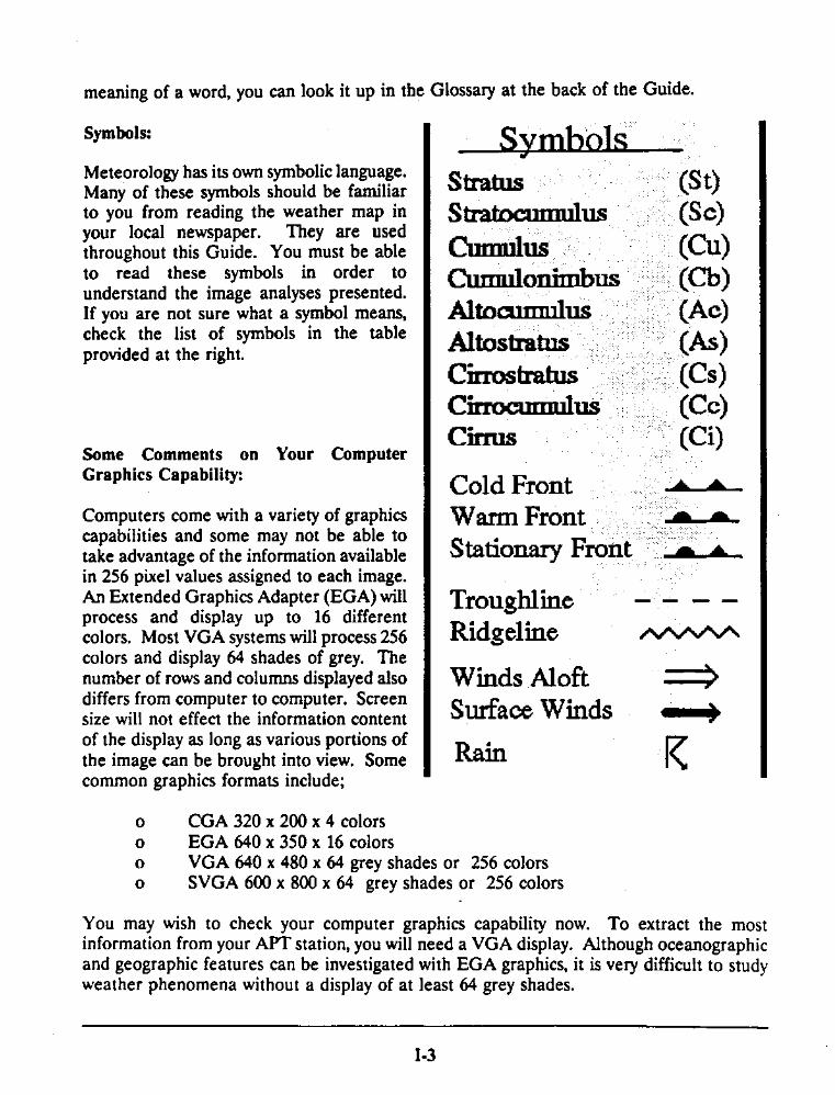
This Guide presents many new words in remote sensing and earth science. Important wordswhose meanings should be learned are printed in bold faced type. If you don’t recall the

I-2

--

_,

Unit 1.0 Remote Sensing Mechanics - Image Processing

1.1 What is a pixel?

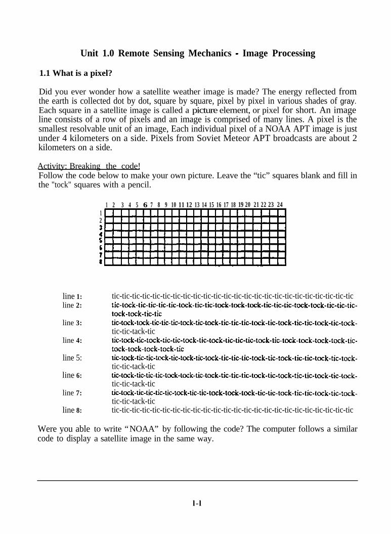
Did you ever wonder how a satellite weather image is made? The energy reflected fromthe earth is collected dot by dot, square by square, pixel by pixel in various shades of gray.Each square in a satellite image is called a picture element, or pixel for short. An imageline consists of a row of pixels and an image is comprised of many lines. A pixel is thesmallest resolvable unit of an image, Each individual pixel of a NOAA APT image is justunder 4 kilometers on a side. Pixels from Soviet Meteor APT broadcasts are about 2kilometers on a side.

Activity: Breaking the code!Follow the code below to make your own picture. Leave the “tic” squares blank and fill inthe "tock" squares with a pencil.

1 2 3 4 5 6 7 8 9 10 11 12 13 14 15 166 17 18 19) 20 21 22 23 2412

i6

:

line 1:line 2:

line 3:

line 4:

line 5:

line 6:

line 7:

line 8:

Were you ablecode to display

tic-tic-tic-tic-tic-tic-tic-tic-tic-tic-tic-tic-tic-tic-tic-tic-tic-tic-tic-tic-tic-tic-tic-tictic-tock-tic-tic-tic-tic-tock-tic-tic-tok-tic-tic-tic-tack-tack-tic-tictic-tock-tock-tic-tic-tic-tock-tic-tock-tic-tic-tic-t~k-tic-t~k-tic-tic-t~k-tic-t~k-tic-tic-tack-tictic-tock-tic-tock-tic-tic-tock-tic-tock-tic-tic-tic-tock-tic-tock-tock-tock-t~k-tic-tack-tack-tack-tack-tictic-tock-tic-tic-t~k-tic-tock-tic-tock-tic-tic-tic-t~k-tic-t~k-tic-tic-t~k-tic-tock-tic-tic-tack-tictic-tock-tic-tic-tic-tock-tock-tic-tock-tic-tic-tic-tock-tic-tock-tic-tic-tock-tic-tock-tic-tic-tack-tictic-tock-tic-tic-tic-tic-tock-tic-tic-tok-tic-tock-tic-tic-tack-tictic-tic-tic-tic-tic-tic-tic-tic-tic-tic-tic-tic-tic-tic-tic-tic-tic-tic-tic-tic-tic-tic-tic-tic

to write “NOAA” by following the code? The computer follows a similara satellite image in the same way.

l-l

1.2 The value of grey shades

Each pixel in an image has a brightness value which can be assigned a grey shade (or color).In the previous example the “tics” were white and the "tocks" were black. Most printed text,like the “NOAA” sign and page you are now reading, is produced in black and white.Although satellite images can be interesting and artistic in black and white, the informationcontained in a picture increases with increasing shades of grey (or color). Notice how theinformation content of the image below increases as more shades of grey are used in theprinting process.

Image 1.1 Increasing the grey shades increases the information in an image display.

As they are transmitted from satellites, each APT pixel has a brightness value ranging from1 to 256 which can be displayed using colors or grey shades ranging from black to white.Each shade relates to the brightness, and thus the physical characteristics of objects withinthe pixel area. A change in grey shade from one pixel to the next adjacent pixel means thatthe brightness has changed, corresponding to a physical change in the scene. If more greyshades are contained in an image display, more changes in physical conditions can bedetected.

1 2 3 4 5 6 7 8 9 10 11 12 13 14 15 16 17 18 19 20Activity: Grey is Informative! 1The graph paper shown here has 15 lines 2and 20 columns. Using a pencil to create :dark and light grey, draw a picture on the Spaper by filling in the pixels. An example :might be a picture of white sky and light 8grey grass with a black tree overlapping 9both. Your picture should have three::shades; black, grey, and white. Can you12imagine your picture in black and white?13 I I I I IDid the grey shade increase the information i I I I I I

content of the image? Discuss what I I I I I

information content would be lost without the three colors.

-

.-

1-2

13 Intermediate Study: Understanding Histograms

Not all 256 brightness values may be present in an image. For example, there may not beanything in a scene that has a very low brightness value that would be displayed using blackor charcoal grey shades. By knowing which brightness values an image contains and howmany pixels of each value, many physical characteristics of objects in an image can bedetermined.

Histograms are statistical graphs of a picture showing the number of shades of grey usedto display the picture and the frequency of occurrence of each shade. Histograms areusually displayed as bar graphs. Each grey shade in a picture is represented by a verticalbar. The height of the bar shows the number of pixels of that shade.

__

The NOAA sign created in “What is a pixel?” contained 8 rows and24 columns totalling 192 pixels. Each of the 192 pixels was either 120black or white. Thus a histogram of the NOAA sign would have twobars. If you count the black pixels you will find that there are 58. 6 0How many are pixels white? A histogram of the NOAA sign lookslike the graph at the right. The height of the bar representing blackpixels is 58 units high. The height of the bar representing white \

pixels is 134 units high.

.

Black Grey White

111Black White

Activity: Histogram Grey is Informative!In the space provided at the left, sketch a histogram of thepicture you created in the “Grey is Information” Activity.Notice that each grey shade corresponds to a different objectin your picture. (Hint: the picture had 15 x 20 = 300 pixels.)

How many bars would the histogram have?

Number of black pixels?

Number of grey pixels?

Number of white pixels?

1-3

Image l.2 Histogram and Soviet Meteor image of the United States’ Gulf Coast.

Image 1.3. The same Meteor image stretched over a range of pixel values from 24 to 64.

1-5

1.5 Summary DiscussionYou have learned that pixels are the fundamental building blocks of a satellite image,defining both the spatial resolution and the brightness (grey scale) of each picture element.The information content of a picture is increased by increasing the number of grey shades.Statistical representations of images in the form of histograms, are helpful in understandingthe content and the changes taking place in an image. Finally, image processing techniqueslike contrast stretching can bring out information content of an image that might nototherwise be apparent.

At this point you have begun to develop skills in handling large volumes of data throughstatistical analyses. You should be able to apply concepts of computer processing to digitaldata analysis. Further exploration of image processing techniques might include finding outhow resolution and scale affect detectability and recognizability of features in a scene.

1-6

Unit 2: Remote Sensing - Electromagnetic Radiation

Remote sensing is the process of collecting information about material objects withoutcoming into physical contact with them. Your eyes are a good example of remote sensors.They collect enormous amounts of information about the world around you without actuallymaking physical contact. Satellite instruments are a lot like eyes. Both rely on waves ofscattered and emitted electromagnetic radiation as their means for gathering information.In this unit you will learn about the nature of electromagnetic radiation and how theradiative properties of the earth and atmosphere are recorded in satellite imagery. Theprinciples of radiation-matter interactions are presented and the radiative properties of fourmajor classes of landscape features - water, clouds, vegetation, and soil - are summarized.This unit serves as the cornerstone for all further exploration of remote sensing.

2.1 Waves are Patterns not Matter

Various types of waves and wave motion are described throughout this Guide. This unitdeals with electromagnetic waves which are detected by satellite remote sensing instrumentsand form the basis for satellite images. The units on weather examine atmospheric waveswhich can have wavelengths that span the entire country. Wave phenomena are also animportant component of ocean circulation, described in unit 7. Some fundamentalcharacteristics of all waves are presented here.

A wave is not a material object but a pattern. A wave can transport energy from one placeto another, but it does not have mass. Some wave patterns are easily visualized. Waterwaves and waves on the strings of musical instruments are two common examples of wavemotion that we can see. Electromagnetic radiation is more difficult to visualize because itconsists of alternating electric and magnetic fields. Examples of radiation include radio andtelevision waves and visible light.

Activity: Visualize a WaveHave your students form two long single lines facing eachother. Students in one line are asked to clap their hands ata constant beat. Each student in the second line is given theinstruction, “Watch the person on your right and do what hedoes one beat later.” Then go to the left end of the secondline and ask the first student to bend his knees and thenstraighten up again. The effect will be a “bump” that travelsdown the line from one end to the other. Yet, not onestudent will have moved either to his left or right showingthat the wave is a pattern without mass.

0, (oooooDooDooDoDo‘+

The most important wave phenomena are not individual “bumps” but repeated identicalwaves. The parts of a repeating wave are defined and shown in the figure on the next page.

2-1

I -Wavelength -1 Ridge - a region of upward displacement.The maximum upward displacement is at thepeak of the wave.Trough - a region of downward displacement.Wavelength - the interval at which the wavepattern repeats itself. Can be measured frompeak to peak or trough to trough.Amplitude - size of the vertical displacementproduced by a wave.Frequency - the number of waves passing agiven point per unit time.

Activity: Measure a Wave. Weather systems move in waves across the country. Weatherwaves can often be visualized in the cloud patterns associated with them. A weather wavehas been drawn on the satellite AFT image shown below.

Place an R on the ridge and a T on the trough.Each degree of latitude is about 100 kilometers long at the earth’s surface. Using this fact,estimate the wavelength and the amplitude of the wave in kilometers. To convert to milesmultiply kilometers by 0.6.

Image 2.1 Illustration of an upper level wave over the Western United States.

2-2

2.2 Electromagnetic Spectrum

All objects that are not at absolute zero temperatureemit electromagnetic radiation in the form of waves ofenergy. Electromagnetic radiation occurs over a continuumof wavelengths from very long radio waves to extremely shortgamma rays. The ordered arrangement of electromagneticradiation as a function of wavelength is called theelectromagnetic spectrum.

We are exposed to a variety of familiar forms ofelectromagnetic waves in our daily lives. A radio stationemits very long radio waves which travel through space andcan be received by radio antennas. Microwaves are shorter,from 10 millimeters to 1 meter, and are used forcommunications. If you hold your hands over a fire or aburner on the oven you are receiving infrared, or heat,radiation. Your eye is sensitive to a small set of wavelengthscalled the visible spectrum, wavelengths from .4 to .75microns. A micron is one millionth of a meter long. At thevery shortest end of the spectrum are ultraviolet rays, X rays,and gamma rays. These are measured in Angstroms or lo-”meters. Astronomers look for energy at these tinywavelengths to learn about the stars.

2.3 Planck’s Law and the brightness of the Sun and Earth

All material objects radiate a continuous spectrum ofelectromagnetic waves that is characteristic of itstemperature. Some portions of this spectrum are brighterthan others. Brightness refers to the radiated energy fluxentering a remote sensor’s field of view from an object.Planck’s radiation law describes the brightness of objects overthe full spectrum of emitted wavelengths. Planck's law states

X-rays

1A

Gamma Rays

that the maximum brightnessof an object occurs at shorter and shorter wavelengths as the temperature of the objectincreases. The relationship between the wavelength and the temperature of an object at itsmaximum brightness can be expressed as;

100 km

l m

10 mm

.75 urn.4 flrn

100 A

ElectromagneticSpectrum

Radio

Microwave

Infrared

visible

Ultraviolet

wavelength(in microns) = 2832 / Temperature(in degrees Kelvin) (eq. 2.1)

where Kelvin (K) is a unit of temperature scaled from absolute zero. Using thisrelationship, it is easy to calculate that the maximum brightness of the sun which has atemperature of 5900 degrees Kelvin (OK), occurs at a wavelength of .48 microns,approximately the middle of the visible region of the electromagnetic spectrum. Thebrightness maximum for the earth and ocean temperature (300°K) occurs at about 9.6

2-3

microns, in the infrared portion of the spectrum.

To measure the temperature of objects on earth, remote sensing satellite instruments oftendesigned to collect electromagnetic radiation in infrared band covering wavelengths between8 to 12 microns. Because the average temperature on earth is about 300°K the earthemits the maximum radiation and has its maximum brightness at these wavelengths.Therefore the signal energy received at the satellite will be the strongest in these bandsunless there is interference as the radiation travels from the earth to the satellite.

Example Problem: The Human Bodv Spectrum!At what wavelength in the electromagnetic spectrum will a human body whose temperatureis 98.6 degrees Fahrenheit emit the most energy (i.e. be brightest)? Hint: The conversionfrom the Fahrenheit scale to the Kelvin scale is

Kelvin = (Fahrenheit - 32) x .5555 + 273.16 (eq. 2.2)

Activity: Hot objects on earth are easilv sensed from satellites that collect energy from theright wavelengths. Many remote sensing satellites including NOAA TIROS-N satellitescollect images over a wavelength band from 3.5 to 4.0 microns. Use the form of Planck'slaw provided in equation 2.1 to calculate the temperature of objects that have theirmaximum brightness in this band of the electromagnetic spectrum. Discuss what kinds ofscenes on earth would have this temperature. It may be helpful to convert Kelvin toFahrenheit using the following equation:

(K - 273.16) x (9/5) + 32 = F (eq. 2.3)

Forest fires, industrial exhaust, and natural gas waste flares have all been detected using the3.7 micron band 3 channel of the AVHRR. Because the pixel resolution for APT satelliteimages is 4 kilometers, these hot spots must either be very hot or very large in order to bedetected.

2.4 The Tiros-N AVHRR is a Radiometer

The camera on the United States TIROS-N satellites is called the Advance Very HighResolution Radiometer (AVHRR). A radiometer is an instrument that measures radiationbrightness within a fixed band of wavelengths. The AVHRR collects images in five spectralbands simultaneously. However APT broadcasts from NOAA satellites contain only twospectral bands. The choice of which bands are broadcast to APT users is made by NOAAand is posted on the NOAA electronic bulletin board. The bands broadcast at any giventime are also encoded within the signal being transmitted from the satellite. Usually, thesolar infrared band 2 and the thermal infrared band 4 are broadcast during the day, andthermal infrared bands 3 and 4 are broadcast at night. The characteristics of the five bandsare shown in Table 2.1. Bands 1 and 2 of the AVHRR instrument collect the sun’selectromagnetic energy as it is reflected off objects within its field of view. Bands 2, 3, and4 collect thermal energy radiated from objects in the infrared portion of the spectrum.

2-4

3

4

s

2

Wavelength (urn)Band

11 58 -0.68

Description Purpose

Visible - green to red Emphasizes cultural features,such as metropolitan areas andcultivated land.

.725 - 1.10 Near infrared Emphas izes l and-wa te rbounda r i e s . Pene t r a t e satmospheric haze.

3.55 - 3.93 Infrared Cloud heights. Transparent towater vapor.

10.30 - 11.30 Infrared Thermal mapping

11.50 - 12.50 Far infrared Thermal mapping. Water vaporcorrection

1 Soviet Meteor Satellites broadcast 0.5 to 0.7 micron image at 2 kilometers resolution.2 The AVHRR on NOAA-10 has only the first four bands.

Table 2.1. Each spectral band on the AVHRR has a special purpose. Bands 2, 3,and 4 are broadcast on NOAA APT channels.

2.5 Reflectance is the Key to Meteor and Band 2 Images

Band 2 collects energy in the solar infrared portion of the electromagnetic spectrum,adjacent to the visible spectrum. Although band 2 is not truly a visible band, the AVHRRdetects the reflection of sun’s light scattered off objects beneath rather than the amount ofradiation emitted from objects due to their temperature. Because the human eye alsodetects reflected sunlight, band 2 is often referred to as a visible band even thoughtechnically it is in the near infrared.

The major classes of features we can see in band 2 images include water, vegetation, soil,and clouds. Weather systems, major water bodies, and soil/vegetation zones can bedistinguished because each of these features has a characteristic reflectance. Each reflects,absorbs and transmits radiation in a different way. When we define the reflectance,absorbance, and transmittance of a feature, we say that we have defined its spectralsignature.

Table 2.2 provides rule-of-thumb reflectance values for four broad classes of landscapefeatures. Low reflectance values mean that these features will appear dark in satellite

2-5

images. Objects with high reflectance values are bright. Because the human eye respondsto light in much the same way as AVHRR band 1 and Soviet Meteor instruments,reflectance properties of materials in this band are “intuitive”. Band 1 images are notbroadcast on the APT link. Until they are enhanced using the procedures learned in Unit1, Meteor images often appear to have only two shades, light clouds and dark earth.

Band 2 is broadcast during the day from NOAA’s AVHRR instruments. Unenhanced band2 images often appear to have three broad classes of objects. Clouds are very bright, landmasses and vegetation are darker, and bodies of water are very dark. Both band 1 and 2images have the most contrast when the sun is high and the contrast will change with theseason.

Table 2.2 Reflectance values for four broad classes of landscape features.

Band Water Vegetation Soil Clouds

1 & Meteor i low (5%)--------_-----WV..- ---_-----__----__i low (l0-30%)-________________i low (l0-30%) i high ( >70%)_________________ __________________2 i low (5%) i medium (50%) i medium (50%) i high ( >70%)

In general the reflectance of land surfaces increases with the extent of development. Forestsappear very dark and cultivated farmlands are somewhat brighter. Urban areas comprisedof concrete are lighter than the surrounding vegetation in band 1 images, but can be darkerin band 2 if the city is set in grasslands or other reflective vegetation.

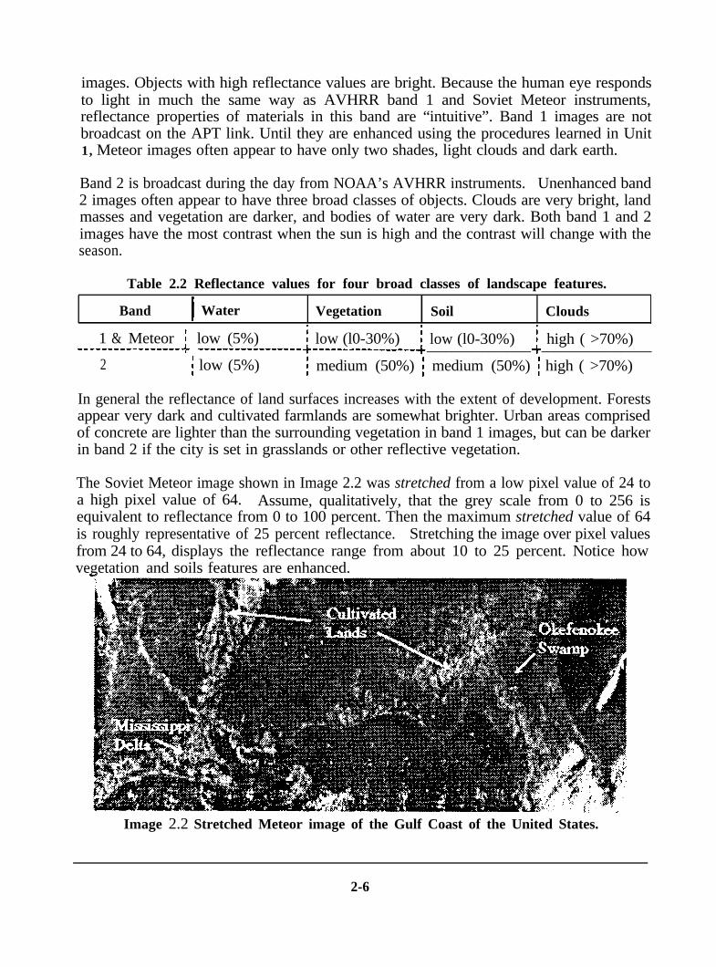
The Soviet Meteor image shown in Image 2.2 was stretched from a low pixel value of 24 toa high pixel value of 64. Assume, qualitatively, that the grey scale from 0 to 256 isequivalent to reflectance from 0 to 100 percent. Then the maximum stretched value of 64is roughly representative of 25 percent reflectance. Stretching the image over pixel valuesfrom 24 to 64, displays the reflectance range from about 10 to 25 percent. Notice howvegetation and soils features are enhanced.

Image 2.2 Stretched Meteor image of the Gulf Coast of the United States.

2-6

This Band 2 image, captured from a NOAA 11 pass on April 26th, 1991 shows theNortheastern United States on a clear spring day. Characteristic of very low reflectance, thedarkest objects in Image 2.3 are water bodies. Many large water bodies are evidentincluding the Atlantic Ocean, Lake Erie, Lake Champlain, and a bit of the Saint LawrenceSeaway. Land areas are an intermediate shade of grey. Land areas that can be easilyidentified include Long Island, Nova Scotia, and Cape Cod. The smaller islands of Martha’sVineyard and Nantucket are also visible. Highly reflective clouds over western New York,Pennsylvania., and New Brunswick are the brightest components of Image 2.3.

-

Image 2.3 Visible (band 2) image of the Northeastern United States on a clear day.

Visible and solar infrared wavelength reflectance of some common materials found on theearth’s surface are described in the following pages. These are provided to give anindication of what values are found in some areas. When examining a specific location indetail, “ground truth” measurements are important. Field trips are a good way of collectingground truth. Aerial photography and resource maps are other important tools. Theseshould be available from the District Department of Interior office in your region.

2-7

Clouds, Snow, and Other Forms of Water:Water in its various states has a dominant influence in all AFT images. In liquid form,water reflects very little of the light incident on it and is consequently the darkest elementin any satellite image. Because cloud droplets scatter sunlight, they appear white in satelliteimages. In general, snow reflects more light than ice does. The liquid water content ofsnow and ice influences spectral reflectance - the greater the water content, the lower thereflectance.

Snow, Ice, Water 1Band 1Fresh dry snow 80 - 90%Wet snow 65 - 75 %Brash and pack ice 35 - 45 %New ice 15 - 25 %Ocean < 5 %Lake water 3 - 10 %Clouds 70 - 75 %

2Band 260-70%50-60%20 - 40 %

< 20 %< 1 %< 5 %

60-70%

Image 2.4 Meteor visible image showing reflectance characteristics of ice, snow and water.

The Soviet Meteor image shown above was captured in early April and shows light snowcover blanketing the northeastern United States and Canada. Lake Nipigon, north of LakeSuperior, and the James Bay are ice-covered and overlain with a dusting of new snow. TheGreat Lakes are not frozen and therefore appear very dark. A layer of thin cirrus cloudscovers the region from Lake Erie to the Saint Lawrence Seaway.

2-8

A common snow pattern seen insatellite imagery is a dendritic pattern.Dendri t ic means a tree-like orbranching pattern. The pattern iscaused by mountain valleys, rivers, andtree lines which contrast sharply withsnow covered areas.

This Meteor image from 21 January,1991 shows dendritic snow patterns inthe western Canadian Rockies. Snowalso covers the Coast Mountains ofBritish Columbia. The flat plains of theSnake River are also apparent. Thediscerning eye can also spot the tops ofnumerous mountains in the Cascadesincluding Mt. Rainier, Mt. Hood andMt. Saint Helens.

Soils:The spectral reflectance of soil iscontrolled for the most part by moisturecontent. Fine clay holds water and isthus less reflective than sand or welldrained silt. Better-drained soils are

Image 2.5 Meteor image showing the dendriticpattern of snow.

more reflective. Particle size distribution also effects reflectance to some extent. Noticethat the finer the particle size, the more reflective the sand.

Band 1 & Meteor Band 2Dark soil 5 - 15 % 10 - 15 %Gray soil 15 - 35 % 10-- 15 %

Dry sand 25 - 50 %Coarse sand 60 - 65 %Medium sand 70 %Fine sand 75 %

Wet sand 15 - 30 %Concrete 15 - 40%

60-80%60-70%

75 %80%

50 - 55 %

This Soviet Meteor image shows the bright fineImage 2.6 Meteor image showing the

sands of Cape Hatteras and the sandy coastlinereflectance of sand and soils

of the Carolinas. Also apparent, are forestedareas in the Great Smoky Mountains and cultivated flatlands along the Atlantic Coast.

2-9

Vegetation:Examples of spectral reflectance values for various vegetation types are shown below.Vegetation is less reflective in band 1 than in band 2. The range of vegetative reflectancevalues from species to species is broader in band 2, ranging from 18 to 80 percent.

Species Band 1 & Meteor Band 2Fir 5 % 18%Pine 10 % 30%Birch 15-25% 50 - 70%Grasslands 20 - 30 % 60-80%

-

-

-

As suggested by the data in the table, coniferous forests are generally less reflective thandeciduous forests, due primarily to the density of water versus air in the leaf structure. Inband 2, healthy deciduous vegetation reflects more light than concrete. Thus urban areasshould appear darker than the surrounding grasslands. Urban areas surrounded by coniferswill appear brighter than their surroundings.

Image 2.7 of Florida illustratesthe importance of water contenton the reflectance of areasbeneath. The Evergladesecosystem depends on freshw a t e r f l o w f r o m L a k eOkeechobee across south Floridainto the Gulf of Mexico. Thepathway for the water flow,called the Shark River Slough, isreadily apparent in this imagebecause it is wetter, and thusdarker, than the surroundinghigher ground.

Vegetative spectral reflectance inband 2 is directly correlated withwater content in the leafstructure. Monocots and youngleaves are generally compact andhave a high water content.Dicots and older leaves have lesswater and more air in theirstructure.

Image 2.7 TIROS-N band 2 image showing thereflectance of everglades vegetation.

The change in reflectance from band 1 to band 2 suggests that the ratios of reflectancemeasured in one band to another might be a very good indication of species.

2-10

-

2.6 Temperature is the Key to Bands 3 and 4

-

--

-

-

-

.-

-

Band 3 and 4 infrared images show temperatures and temperature differences of thelandscape beneath. Cold objects appear bright and warm objects are dark.

Image 2.8 is a thermal infrared image from NOAA 10. The darkest areas of the image arethe warmest and the lightest areas are the coldest. The coldest objects in the image areclouds. The circular cloud pattern centered over Missouri and Illinois is a low pressuresystem. Low pressure systems are correlated with stormy weather which is fed by the mixingof warm and cold air masses. A warm tongue of air from the Gulf of Mexico is feeding thefrontal system followed by colder air over Kansas and Oklahoma which is entering thesystem from the west. The Gulf Stream current is a warm water current in the AtlanticOcean. It is visible in this image located about 100 kilometers off the coast of Virginia.You can estimate distances on images that have latitude and longitude markings byremembering that one degree latitude is about 100 kilometers.

Image 2.8. In thermal infrared images, warm features are black and cold objects are white.

2-11

Infrared remote sensing depends on detecting the radiation emitted from objects in a scenerather than on radiation from reflected sunlight. Thermal energy emitted from the earthand ocean is a maximum in the wavelength intervals between 10 and 11 microns. Brightnessvalues measured in band 4 are almost linearly dependent on temperature, and thus grey-shade steps in an image are uniform temperature steps as well. The relationship betweenbrightness and temperature is not quite linear for band 3. APT images are broadcast withcalibration data for converting measured brightness values to temperatures.

The band 4 infrared image below shows two large hurricanes named Herman and Iselle.They are fed by the warm water of the Pacific Ocean beneath them. The wind speed nearthe center of Herman measured 150 knots. Winds near the center of Iselle measured 100knots. You can use the latitude and longitude lines to estimate the diameter of the eye ofeach hurricane. The smaller very cold cloud masses over the Gulf of California andsoutheastern Arizona are thunderstorms. The desert areas of southern California and theBaja Peninsula appear very warm. Tropical storms are covered more extensively in Unit 6 -Weather Systems.

Image 2.9 TIROS-N infrared image of twin hurricanes off the West Coast of Mexico.

2-12

T8ctwl = Tbrightnerr e-l’*

2.7 Intermediate Study: Black Body Radiation

A black body is an object that emits an amount of radiation equal to the amount it absorbs.Only black bodies are perfect emitters of radiation; most real objects are not. Most objectsradiate somewhat less energy than if there were perfectly black. The parameter relatingthe observed brightness of an object to an ideal black body emitter is termed emissivity.Emissivity (e) is defined as the ratio of the observed brightness (Bob__Jto the ideal energyflux (B,,,,,). The actual temperature of an object is

(es 2.4)

Because remote sensing instruments like the AVHRR measure the brightness temperaturesof objects in a scene, the emissivity of the object is required in order to derive the actualtemperature.

Surface emissivities of some common materials are shown in the Table 2.3. Calculationsof actual temperature and brightness temperature have been entered in the Table for theextreme cases of asphalt and water. You should complete the table as an exercise.. Note thatactual temperatures are warmer than measured temperatures. Brightness temperatures ofdark rocks can be in error by as much as 10°K. However for water, the difference betweenthe temperature measured by the satellite and the actual temperature is within 1°K.Therefore satellite derived ocean temperatures should be quite accurate without correctingfor emissivity of water.

The importance of emissivity to accurate measurement of surface temperature can be notedby observing that a one percent change of emissivity produces a change in surfacetemperature of slightly under 1° Kelvin. Therefore, in order to measure the temperatureof an object on earth to within lo, emissivity must be known to within one percent.

Table 2.3 Emissivity and Brightness Temperature of Selected Materials.1

T- if T- is 300° T- if T,, is 300°Material e eY4 Kelvin Kelvin.

Rock: Asphalt 0.86 0.963 311.5° Kelvin 288.9° K

Granite 0.90 0.974 308.0° K

Basalt 0.92 0.979

Concrete 0.97

Soil: Dry sand 0.91 0.977

Wet sand 0.94 0.985 304.6° K

Water:Ice 0.95 0.987 303.9° K

Fresh/Salt 0.99 0 . 9 9 7 300.9° K 299.1° K

2-13

Activity: Infrared PhotographyInfrared film is available for 35 mm cameras at most professional camera shops. Try takingpictures from high places of grassy parks, asphalt playgrounds, water bodies and otherlandscapes. Have the film developed and make comparisons with AFT imagery. Try thisday and night. What changes? What remains the same?

2.8 The Atmosphere’s Content

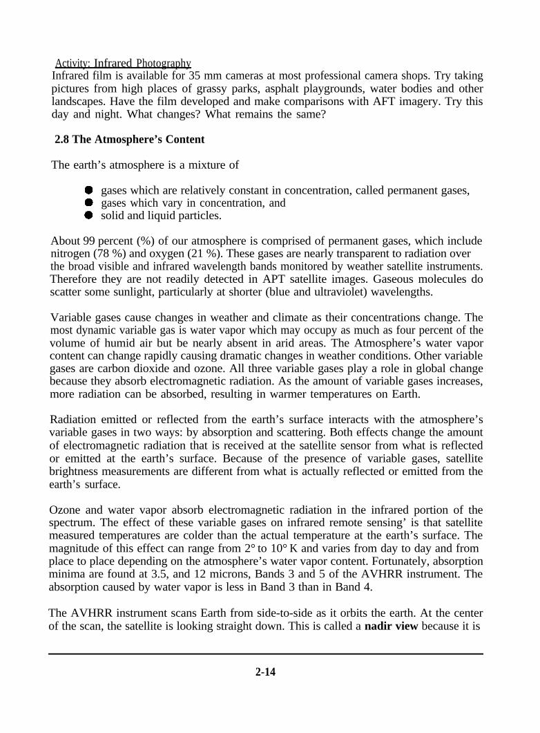
The earth’s atmosphere is a mixture of

aaa

gases which are relatively constant in concentration, called permanent gases,gases which vary in concentration, andsolid and liquid particles.

About 99 percent (%) of our atmosphere is comprised of permanent gases, which includenitrogen (78 %) and oxygen (21 %). These gases are nearly transparent to radiation overthe broad visible and infrared wavelength bands monitored by weather satellite instruments.Therefore they are not readily detected in APT satellite images. Gaseous molecules doscatter some sunlight, particularly at shorter (blue and ultraviolet) wavelengths.

Variable gases cause changes in weather and climate as their concentrations change. Themost dynamic variable gas is water vapor which may occupy as much as four percent of thevolume of humid air but be nearly absent in arid areas. The Atmosphere’s water vaporcontent can change rapidly causing dramatic changes in weather conditions. Other variablegases are carbon dioxide and ozone. All three variable gases play a role in global changebecause they absorb electromagnetic radiation. As the amount of variable gases increases,more radiation can be absorbed, resulting in warmer temperatures on Earth.

Radiation emitted or reflected from the earth’s surface interacts with the atmosphere’svariable gases in two ways: by absorption and scattering. Both effects change the amountof electromagnetic radiation that is received at the satellite sensor from what is reflectedor emitted at the earth’s surface. Because of the presence of variable gases, satellitebrightness measurements are different from what is actually reflected or emitted from theearth’s surface.

Ozone and water vapor absorb electromagnetic radiation in the infrared portion of thespectrum. The effect of these variable gases on infrared remote sensing’ is that satellitemeasured temperatures are colder than the actual temperature at the earth’s surface. Themagnitude of this effect can range from 2° to 10° K and varies from day to day and fromplace to place depending on the atmosphere’s water vapor content. Fortunately, absorptionminima are found at 3.5, and 12 microns, Bands 3 and 5 of the AVHRR instrument. Theabsorption caused by water vapor is less in Band 3 than in Band 4.

The AVHRR instrument scans Earth from side-to-side as it orbits the earth. At the centerof the scan, the satellite is looking straight down. This is called a nadir view because it is

2-14

84 percent of the light reflected from the surface in band 2 will reach the satellite. Sincethe sunlight being reflected has to travel two ways through the atmosphere (down and back),the probability of two way transmission is Ta2 or 0.71.

Example Problem 1:Using a typical hazy day optical thickness of .7 for band 2, calculate the two waytransmittance of the atmosphere on hazy days.

Example Problem 2:A typical cirrus cloud is about 1 kilometer thick and 75 percent of all cirrus clouds are lessthan 2 km thick. The total two way propagation path for near infrared light through cirrus clouds can be calculated from the following model equation:

T,’ = exp[-.28 L2] (eq. 2.6)

where L is the thickness of the cirrus layer in kilometers. What is theprobability for a 1 kilometer thick cirrus cloud?

two way transmission

2.10 Summary Discussion

The materials presented in Unit 2 are fundamental to remote sensing and are a prerequisiteto comprehending the information content of any remotely sensed scene. The objective ofthis unit was to build an understanding of electromagnetic radiation and the relationshipbetween electromagnetic energy flux and remote sensing signatures. The concepts of wavesand wave motion have been presented as have been the nature of electromagnetic radiationand radiative transfer. You should be able to define the parts of a wave and relate theseparts to the electromagnetic spectrum.

You have learned that waves of electromagnetic energy are reflected and emitted from allobjects in different quantities depending on the object’s material content and physicalcharacteristics. You should be able describe the relationship between and object’sreflectance, its temperature, and its brightness as recorded in satellite imagery. By knowinghow the reflectance and temperature of material objects influence the appearance ofsatellite images, you should be able to recognize major features in an image and be able tointerpret and compare visible and infrared images.

The influence of scattering and absorption by gases in the atmosphere on the quality ofsatellite images of Earth has been examined. This advanced topic of radiative transferthrough the atmosphere can be explored in much greater depth than presented here,particularly as it relates to global change and warming.

This Unit should challenge the resourcefulness and academic capacities of its readers.Opportunities for problem solving in physics, geography, geometry, algebra, and statistics areabundant.

2-16

-

Unit 3: The State of the Atmosphere - How Clouds Form

-

-

-

3.1 Temperature and Atmospheric Circulation

Temperature differences from place to place on the earth’s surface result in convective airflow, or winds. When a gas is warmed its volume expands and it tends to rise. You canobserve this on a small scale by placing your hand over a pan of boiling water or bymeasuring the air temperature at the top and the bottom of a heated or air conditionedroom. The physical law that states that the volume of a gas is proportional to itstemperature is called the ideal gas law. The mathematical relationship is the equation ofstate. The equation of state is presented in section 3.3.

Global wind patterns begin when air at the equator isheated by the sun. This hot humid air expands andrises to a height of about 20 kilometers (12 miles). Itthen flows toward the colder polar regions where itsinks again at about 30 degrees latitude. The regionsof sinking on either side of the equator are calledsubtropical high pressure areas. Because of theearth’s rotation underneath the atmosphere, low levelair flow back toward the equator appears to have aneasterly (from the east) orientation. These easterliesare called trade winds. Winds flowing away from theequator from the subtropical high are calledwesterlies. Westerlies occur in the mid-latitude bandsof the earth.

C-\ rising

Thermometers for measuring temperature are scaled by the melting point of ice and theboiling point of water. On the Celsius scale, the difference between the boiling and freezingis divided into 100 parts, or degrees Celsius (°C), where zero is freezing and 100 is boiling.On the Fahrenheit scale, the difference between freezing and boiling is divided into 180parts or degrees Fahrenheit (° F). The temperature of melting ice is marked at 32° F andboiling water at 212° F. The universal temperature scale is called the Kelvin scale. Degreeson the Kelvin scale are equivalent to degrees on the Celsius scale. However, zero on theKelvin scale is set at absolute zero, the temperature at which molecules stop moving andthere is no heat at all. Zero degrees Kelvin is -273.16° C or -459.4° F.

3.2 Pressure and Atmosphere

Air has weight. One simple way to prove it is to balance two balloons on a yard stick. Prickone and watch what happens. The weight of the atmosphere over a one inch square patchof land at sea level is 14.7 pounds. Using this information you can compute that the weightof air on your shoulders (about 1 square foot or 144 square inches) is over one ton! Wedon’t feel it because we are used to it.

3-1

Pressure is defined in terms of the weight of the atmosphere per unit area. Semi-permanenthigh and low pressure areas occur at various locations on earth. These locations are relatedto the global circulation pattern described above. Over the equator, where moist tropicalair rises due to the sun’s heating, is a permanent belt of low pressure called the IntertropicalConvergence Zone (ITCZ). At 30 degrees north and south of the ITCZ are belts of highpressure called subtropical highs. Semi-permanent high pressure systems also reside overeach of the poles. These two high pressure areas are separated by a low pressure beltsometimes called the polar front. The polar front occurs at about 60 degrees latitude butmeanders toward the equator during the cold season. These high and low pressure belts aremarked on the figure above.

Atmospheric pressure is measured with a barometer. One common type of barometerconsists of a glass tube about 800 millimeters long. The tube is filled with mercury,inverted, and placed in a dish of mercury. The level of mercury falls until the force per unitarea on the mercury in the dish supports the mercury in the tube. At sea level about 760millimeters of mercury should remain in the tube. As the atmospheric pressure on themercury in the dish rises and falls, the mercury level in the tube will rise and fall.

Pressure is sometimes reported in fractions of normal sea-level atmospheric pressure, orfractions of an atmosphere (atm). On this scale, 1 atm is the weight per unit area of theatmosphere above land at sea level. Units of pressure which are equivalent to 1 atm are1013.25 millibars, or 760 millimeters of mercury or 29.9213 inches of mercury.

3.3 Thermodynamics

Atmospheric pressure decreases with height above the earth. Our bodies detect changes inatmospheric pressure when they take place. You may have experienced the effects ofpressure drop with height causing your ears to pop as you drive over a mountain.Meteorologists often report the height of weather phenomena above the earth’s surface inunits of pressure rather than length. The relationship that describes how pressure changeswith height is called the hydrostatic equation. A simple form of this equation, which is onlyvalid near the surface of the earth where the density of the air is also constant (about thefirst 5 kilometers), can be written as follows:

Pat height h = 1013 -h/10

where P is pressure in millibars and the height h is measured in meters, the value of theconstant is 10. The hydrostatic equation was used to develop the conversion ruler shownon the next page. You may wish to develop a conversion ruler from “millibars” to “feet” asa classroom activity.

The study of the solid, liquid, and gaseous states of a system is called thermodynamics.The properties of state. sometimes called the variables of state, are pressure, temperature,and volume. The equation of state defines the relationship between state variables when a

3-2

1013 mb 700 mb 500 mb 400 mb 300 mbt . I . . I . 40 1 km 3 km 5km 7km 9 km

b 8 I I * . I I I 8 i

0 mi 1 mi 2 m i 3 mi 4 mi 5 mi 6 mib I I I I 4 1

system is in equilibrium. The equation of state for a constant fixed volume of gas is:

Pressure(millibars) x Volume = Constant x Temperature(Kelvin) (eq. 3.2)

In section 3.1 we explained the relationship between the temperature of a gas and itsvolume. The equation of state also says that if the pressure on a gas is increased, the gaswill heat and if the pressure decreases, that gas cools. This law explains why a bicycle pumpfeels hot when it compresses air, and why a fire extinguisher gets frosty cold when it is used.For meteorological purposes, the ideal gas law when combined with the hydrostatic equationstates that the temperature of the atmosphere must decrease with altitude.

As a general rule, the temperature of dry air decreases at a rate of 10” C per kilometerabove the ground. This is called the dry adiabatic lapse rate. The temperature of saturatedair decreases more slowly, at a rate of about 5” to 7” C per kilometer. Meteorologists referto this as the moist adiabatic lapse rate. The term adiabatic refers to a thermodynamicprocess which takes place without gain or loss of heat.

3.4 Water Vapor

The atmosphere’s water content varies in time and place. Because water at atmospherictemperature readily changes state from solid ice to liquid drops to gas, it can be easilypicked up, transported, and deposited from place to place around the world. Dry air soaksup water by converting it to its gaseous state, called water vapor. However, like a spongewhich cannot hold an unlimited amount of water, theatmosphere cannot hold an unlimited amount of watervapor. The maximum possible amount a volume of aircan hold depends on temperature and pressure. Thehigher the temperature or the pressure, the more watervapor air can hold.

Saturation

evaporating = condensingmolecules molecules

air 0 u. . . . . . . . . . . . . . . . . . . . . . . . . . . . . . . . .w91tetizi:&:.: . . . . . . . , ..*.*.. .,.,.,::A .:,. . ..;,: ~:::~:i.:.i.:...:.:::::.:.:,:.:::l’ig . .::*:::<::: ,.,.,.,.....,.,.. < .,.,...,.,.,.,.....,.,.,.......,. :.:.~~~~:.~,:.~:.~:.:~~~~~:::::.:.:,::::::::::::::h5:::::~.:.:.~:.:.:.~::::::::::~:.:.............~;liryiiiiiiiiiiiiiiiiirijijiiiiiiliili~I:i:i::::~~.:.~:.~~:~:~~::.~~~:~:~:~:~ .,.......... , . . . . . .> .:.:.:.: > :., :.:.:.:.:.:d~.‘........ ..A **& :.z$$>U: . ,‘.‘..,.....~..:.:.:.~~.‘.:.:.:.:,:~.:,:,:~,’,’,‘,’ +>:. . ..n.+>..:.:.:.. :. . . . . . . ..:.:.:,::::::::::::::::‘..,....,.: $:::::::::\.:.:.:*:::.:.:.:.:.:,::::.’ ” ‘,’t$<:$*::::$$...~.,~:‘:.:‘:~~.:.:.~~:.: ,,.:,c,‘.....s l ..*.... ~..::~:!!:~l::.:‘:.:~~:~~..a * . . . . . . . A, . 4. . . . , , . . ..>..‘...A... ..A . . . ..%..*r..hw.<...s.~4...:+..:.:.:.:., . . . . .<*:::::*::::::::

-

--

--

Perhaps you have noticed how sidewalks dry out in thesun after a rain, or how water condenses on grass oncold evenings. This figure depicts an air water interface. Water molecules can evaporateleaving the water and entering the air and they can condense from the air back into thewater. Saturation occurs when evaporation equals condensation. The temperature to whichair must be cooled to reach saturation is called the dew point temperature. If air is cooled

3-3

beyond the dew point, then the excess water vapor condenses into droplets. If thetemperature rises above the dew point, then water will evaporate.

Relative humidity is another measure of the air’s water vapor content expressed as the ratioof the actual atmospheric water vapor to the maximum possible. If a volume of air with arelative humidity of 50 % is cooled, the relative humidity will increase until it reaches 100%. Further cooling will result in fog, rain or another form of precipitation.

3.5 How Clouds Form

Clouds form when moist air cools beyond its dew point temperature and the excess watervapor condenses. There are two main ways to cool air to bring about condensation;radiative cooling and adiabatic expansion as a result of vertical motion. The various causesof vertical motion include; lifting of air over mountains, convection caused by the sun’sunequal heating at the earth’s surface, convergence of air flow, and frontal ascent oradvection. Clouds dissipate either when air is heated above its dew point, or if the moisturefalls out as precipitation.

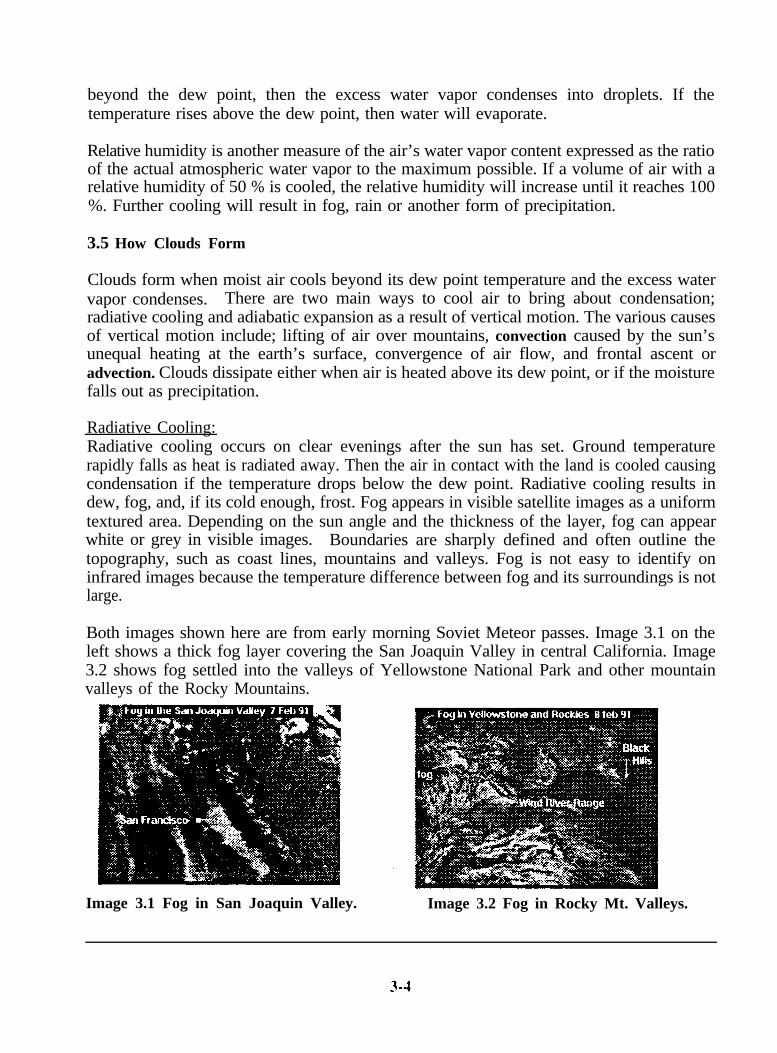
Radiative Cooling:Radiative cooling occurs on clear evenings after the sun has set. Ground temperaturerapidly falls as heat is radiated away. Then the air in contact with the land is cooled causingcondensation if the temperature drops below the dew point. Radiative cooling results indew, fog, and, if its cold enough, frost. Fog appears in visible satellite images as a uniformtextured area. Depending on the sun angle and the thickness of the layer, fog can appearwhite or grey in visible images. Boundaries are sharply defined and often outline thetopography, such as coast lines, mountains and valleys. Fog is not easy to identify oninfrared images because the temperature difference between fog and its surroundings is notlarge.

Both images shown here are from early morning Soviet Meteor passes. Image 3.1 on theleft shows a thick fog layer covering the San Joaquin Valley in central California. Image3.2 shows fog settled into the valleys of Yellowstone National Park and other mountainvalleys of the Rocky Mountains.

Image 3.1 Fog in San Joaquin Valley. Image 3.2 Fog in Rocky Mt. Valleys.

Orographic Lifting:Meteorologists call the rise of air as it flows over topographic barriers is called orographiclifting. The temperature of dry air decreases at about lo” C per kilometer as it is lifted.If the air cools beyond its dew point temperature, then condensation takes place and cloudsform. Saturated air cools at a little more slowly as it is lifted because when water vaporcondenses it gives off a bit of extra heat, called latent heat. Therefore, saturated air coolsat rate of about 5” to 7° C per kilometer.

Activity;In the figure shown here, an air parcel on theupwind side of the mountain has a temperatureof 25°C and the mountain is 4 kilometers high.As air is lifted with the air flow, it cools at arate of 10°C per kilometer. At a height of 3kilometers it reaches the dew pointtemperature (-5°C) and clouds form. The airparcel continues to rise and cool at a saturatedrate of about 6°C per kilometer. What is thetemperature at the top? Descending down the

leeward side of the mountain it heats up at a rate of 10°C per kilometer to 29°C at thebase. The air parcel is both warmer and drier on the leeward side of the mountain.

Cloud formation due to orographiclifting is readily apparent in both visibleand infrared images. The effects of theAppalachian mountains on cloudformation is clearly depicted in thisNOAA 11 APT satellite image capturedon February 11th 1991. This is arelatively clear cold day.

Image 3.3 Clouds form due to orographic liftingover the Blue Ridge Mountains.

3-5

Image 3.4 Cloud dissipation on the leeward sideof the Sierra Nevadas.

Image 3.4 of the western United States,was captured from a NOAA 10 pass onMarch 10, 1991. Moist air from thePacific Ocean is lifted up the west sideof the Sierra Nevadas in easternCalifornia. As it lifts it cools below itsdew point temperature and water vaporcondenses forming clouds. The air massdrys out as it descends down the otherside of the mountains into Nevada.

An unusual variation of orographiceffects is shown in Image 3.5. Here, airis constrained by high mountain rangesto the north and south, forcing it to passthrough the Casper Gap in centralWyoming. As moist air approaches thegap it converges and is forced to risecausing the cloud formation seen in thisimage.

-

-

Image 3.5 Lifting due to converging air as it passes through the Casper Gap,

3-6

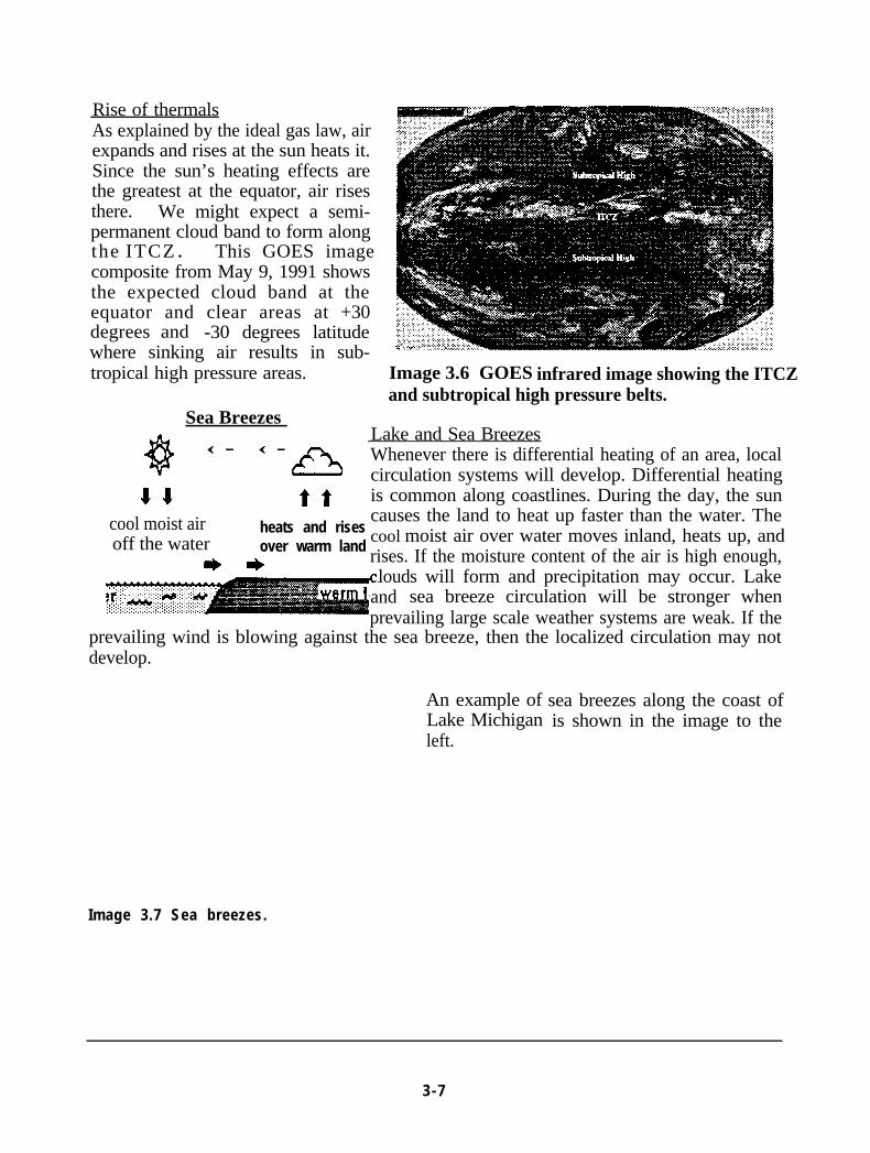
Rise of thermalsAs explained by the ideal gas law, airexpands and rises at the sun heats it.Since the sun’s heating effects arethe greatest at the equator, air risesthere. We might expect a semi-permanent cloud band to form alongthe ITCZ . This GOES imagecomposite from May 9, 1991 showsthe expected cloud band at theequator and clear areas at +30degrees and -30 degrees latitudewhere sinking air results in sub-tropical high pressure areas. Image 3.6 GOES infrared image showing the ITCZ

and subtropical high pressure belts.Sea Breezes

Lake and Sea Breezes‹- ‹-

AWhenever there is differential heating of an area, localcirculation systems will develop. Differential heating

$4 tt is common along coastlines. During the day, the suncool moist air heats and rises

causes the land to heat up faster than the water. Theoff the water over warm land cool moist air over water moves inland, heats up, and

I) * rises. If the moisture content of the air is high enough,louds will form and precipitation may occur. Lake

and sea breeze circulation will be stronger whenprevailing large scale weather systems are weak. If the

prevailing wind is blowing against the sea breeze, then the localized circulation may notdevelop.

An example ofLake Michiganleft.

Image 3.7 Sea breezes.

sea breezes along the coast ofis shown in the image to the

3-7

Another example of differential heating resulting in cloud formation is when coldcontinental air flows offshore over the warmer ocean water. As the cold air reaches thewarm water it rises resulting in stratus or strato-cumulus cloud streaks (see Unit 5 for moreon cloud types). As shown in Image 3.8 from NOAA 10 captured on March 11th, 1991 thecloud edge off the east coast is often a good predictor of the location of the warm watersof Gulf Stream. Other feature of this image include some topographic cloud formation overthe Great Smoky Mountains and a glimpse of the Shenendoah Valley. A light dusting ofsnow streaks the countryside from Michigan through West Virginia. The Great Lakes appearto be warmer than the surrounding land indicating not only that this is a cold day but thespring is on its way.

-

-

_

Image 3.8 Cold continental air rising over warm Gulf Stream water.

3-8

-

-

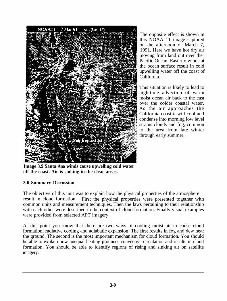
Image 3.9 Santa Ana winds cause upwelling cold wateroff the coast. Air is sinking in the clear areas.

The opposite effect is shown inthis NOAA 11 image capturedon the afternoon of March 7,1991. Here we have hot dry airmoving from land out over thePacific Ocean. Easterly winds atthe ocean surface result in coldupwelling water off the coast ofCalifornia.

This situation is likely to lead tonighttime advection of warmmoist ocean air back to the eastover the colder coastal water.As the air approaches theCalifornia coast it will cool andcondense into morning low levelstratus clouds and fog, commonto the area from late winterthrough early summer.

3.6 Summary Discussion

The objective of this unit was to explain how the physical properties of the atmosphereresult in cloud formation. First the physical properties were presented together withcommon units and measurement techniques. Then the laws pertaining to their relationshipwith each other were described in the context of cloud formation. Finally visual exampleswere provided from selected APT imagery.

At this point you know that there are two ways of cooling moist air to cause cloudformation; radiative cooling and adiabatic expansion. The first results in fog and dew nearthe ground. The second is the most important mechanism for cloud formation. You shouldbe able to explain how unequal heating produces convective circulation and results in cloudformation. You should be able to identify regions of rising and sinking air on satelliteimagery.

3-9

Unit 4: Cloud Types - How Do We Recognize Them

The most common features seen on meteorological satellite images are clouds and cloudsystems. In this Unit you will learn to recognize cloud types and determine their nature,extent, height and movements. You will be shown how separate out low, middle and highclouds, and to determine the height and intensity of weather phenomena by comparingvisible and infrared imagery.

4.1 Classifying Clouds

Nine cloud types presented in this unit are listed in the table below. The abbreviatedsymbols in the table are used to denote cloud types and mark them on satellite images.Clouds are generally classified by

0 shape,0 content, and0 height above the ground.

Cloud Shapes:There are two main categories ofcloud shape; cumuliform andstratiform.

Cumuliform, or heap, cloudslook like fat puffy cotton balls.They can be fair weatherindicators. They are likely tohave strong vertical motionswithin them and they can haveconsiderable vertical depth.Cumuliform clouds develop in anunstable atmosphere. Theirappearance on satellite images isvisual evidence of convection in the atmosphere.

Stratiform clouds are layered and spread like sheets across the sky. They develop in a stableatmosphere and generally have less vertical motion and less turbulence associated withthem. When they appear in satellite images they give evidence of widespread cooling,usually as a result of advection of moist air over a cooler air mass or land surface beneath.

Cloud content:Clouds contain water, ice, or a mixture of both. Cumulus (Cu) and stratus (S) clouds arefairly warm, usually above 0” C, and comprised of water. Water clouds can be distinguishedin satellite images by their sharp boundaries. Clouds composed of a mixture water droplets

4-1

and ice crystals are known as mixed clouds. Mixed clouds are usually undergoing strongvertical development, such as that which occurs in thunderstorm clouds called cumulonimbus(Cb) clouds. Below -38° C only ice crystals form by condensation. Ice crystal clouds, whichhave fibrous structure, are easily identified in satellite images. They look like they havebeen painted on with a dry brush. Cirrus clouds are made of ice crystals.

Cloud Height:The third way of classifying clouds is by their average base height above the ground.Meteorologists speak of three main height categories; low clouds, middle clouds and highclouds. Low clouds are those that have base heights from the earth’s surface up to about2,000 meters (about 6,500 feet). Middle clouds are found between about 2,000 and 6,000meters (6,500 to 20,000 feet), and high clouds are higher than about 6,000 meters (20,000feet) above the ground. The cloud layer of the atmosphere stops at about 15 to 18kilometers (10 miles or 60,000 feet). This layer of the atmosphere is known as thetroposphere. Base heights described here are representative of mid-latitudes. In the tropics,base heights are a bit higher and they are lower near the poles.

Because the atmosphere cools with height, cloud temperatures also decrease with height.Meteorologists have found that the temperature at the base of low clouds is usually in therange between 0” and 25° C. The base temperature of middle clouds ranges from 0°C to -25° C and high cirrus clouds are almost always colder than -25” C. Of course satellitesmeasure temperature at the top of a cloud, not its base. Nevertheless, cloud toptemperatures can be used to help identify cloud types. Because stratiform clouds do notdevelop vertically, their tops are likely to be lower and warmer than cumuliform clouds.Cumuliform clouds are accompanied by strong vertical development. Depending on thestrength of convective activity, the tops of cumuliform clouds can extend through the entiretroposphere. The tops of Cumulonimbus (Cb) thunderclouds are often colder than -50°C.In Image 4.1 pixels in the temperature range from -50°C to -55” C are blackened.

Image 4.1 Cloud height relates to temperature on infrared images.

4-2

In visible satellite images the brightness of clouds depends on cloud thickness and the sun’sangle of reflection off the cloud tops. Thick clouds have roughly equal brightness in visibleimagery regardless of their height or content. Very thin clouds can appear grey becausethey are partially transparent. Not all of the sunlight is reflected back toward the satellitesensor. Sunlight is readily transmitted through thin cloud layers. (Refer to Unit 2, section9 for a more detailed discussion of cloud transmittance.) High icy clouds are most likely tobe thin and appear grey in visible satellite imagery.

In thermal satellite images (AVHRR bands 3 or 4), the brightness of clouds depends ontemperature. Ice clouds like cirrus (Ci) are cold and appear much brighter than cloudscomprised of warmer water like fog and stratus (S). Because the atmosphere’s temperaturedecreases with height, higher clouds are almost always colder than low level clouds.Therefore, the temperature of cloud tops as determined by the brightness of infraredimagery provides a qualitative measure of cloud height. When visual imagery is usedtogether with thermal infrared imagery, cloud discrimination is most easily accomplished.

Date:. uov 12 Cloud Photo # aTime: 9:30 sawLocation: Sd-l Camera Direction:

NNEE@s SW w NW

Istratiform _cllmulifom_s@lCbAs

AC Cs Cc Ci

Wind Speed: 4 “+‘I&Wind Direction: S ETemp:* P&p:-Pressure: 2 9. 8 cRH: $3 .f,,

Activity: Cloud Atlas The best way to become familiar with cloud types and to relate themto weather is to create your own cloud atlas. The materials needed include a camera, 3 x5 cards, photo-album, compass, and a cloud chart available from the National WeatherService. Photograph clouds and collect data on 3 x 5 cards in a format similar to the oneshown here. Initially, it will seem like there are an endless variety of cloud types. However,before long patterns will become apparent and you will be able to identify and classifyclouds quickly. By including surface weather conditions in your log, you will learn to relateeach cloud type to impending weather. The data cards should be mounted in the album onthe same page as the photo.

4-3

4.2 Low Clouds

Low clouds occur in the lowest level of the atmosphere.above 2,000 meters (6,500 feet). These clouds includestratocumulus (SC) types.

Their heights do no generally reachfog, stratus (S), cumulus (Cu), and

Stratus (S) and fog are the lowest cloud types. The only difference between the two is thatfog touches the ground. Both are caused when air near the ground cools after sunset orwhen warm air is advected over cooler land, water or air near the ground. Advection is theprocess of heating or cooling an air mass by transporting it horizontally over an area ofdifferent temperature. From a satellite’s vantage point, fog and stratus clouds look thesame. They both look uniform in shade and they have very little texture although theiredges are sharply defined. In visible images, brightness depends on cloud thickness and sunangle. A thick stratus layer will appear very bright.

In infrared images, stratus and fog appear grey. They can be hard to distinguish frombackground because their temperature is not much different than their surroundings. Infact, the air on the top of stratus and fog layers is often warmer than the cloud layer itself.This is caused when upper level air sinks down on top of the fog layer and is called asubsidence inversion or temperature inversion. Infrared Image 4.2 shows stratus cloudsblanketing most of northern and central Florida. Other low level clouds; stratocumulusstreaks and open cell cumulus clouds are also visible.

Image 4.2 Infrared view of low level cumuliform and stratiform clouds.

4-4

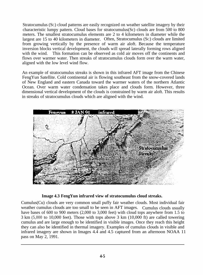
Stratocumulus (SC) cloud patterns are easily recognized on weather satellite imagery by theircharacteristic lumpy pattern. Cloud bases for stratocumulus(Sc) clouds are from 500 to 800meters. The smallest stratocumulus elements are 2 to 4 kilometers in diameter while thelargest are 15 to 40 kilometers in diameter. Often, Stratocumulus (SC) clouds are limitedfrom growing vertically by the presence of warm air aloft. Because the temperatureinversion blocks vertical development, the clouds will spread laterally forming rows alignedwith the wind. This formation can be observed as cold air moves off the continents andflows over warmer water. Then streaks of stratocumulus clouds form over the warm water,aligned with the low level wind flow.

An example of stratocumulus streaks is shown in this infrared AFT image from the ChineseFengYun Satellite. Cold continental air is flowing southeast from the snow-covered landsof New England and eastern Canada toward the warmer waters of the northern AtlanticOcean. Over warm water condensation takes place and clouds form. However, threedimensional vertical development of the clouds is constrained by warm air aloft. This resultsin streaks of stratocumulus clouds which are aligned with the wind.

Image 4.3 FengYun infrared view of stratocumulus cloud streaks.Cumulus(Cu) clouds are very common small puffy fair weather clouds. Most individual fairweather cumulus clouds are too small to be seen in AFT images. Cumulus clouds usuallyhave bases of 600 to 900 meters (2,000 to 3,000 feet) with cloud tops anywhere from 1.5 to3 km (5,000 to 10,000 feet). Those with tops above 3 km (10,000 ft) are called toweringcumulus and are large enough to be identified in visible images. Once they reach this heightthey can also be identified in thermal imagery. Examples of cumulus clouds in visible andinfrared imagery are shown in Images 4.4 and 4.5 captured from an afternoon NOAA 11pass on May 2, 1991.

4-5

-

-

-

-

-

-

-

- Image 4.4 Visible image of various cumulus and stratus clouds over the Northeast.

-

-

-

--

- Image 4.5 Infrared image of cumulus and stratus cloud forms.

-

4-6-

-

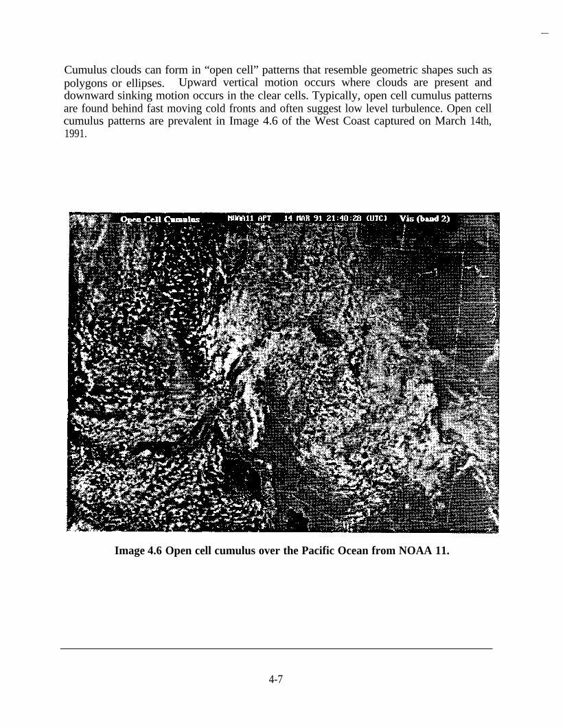
Cumulus clouds can form in “open cell” patterns that resemble geometric shapes such aspolygons or ellipses. Upward vertical motion occurs where clouds are present anddownward sinking motion occurs in the clear cells. Typically, open cell cumulus patternsare found behind fast moving cold fronts and often suggest low level turbulence. Open cellcumulus patterns are prevalent in Image 4.6 of the West Coast captured on March 14th,1991.

Image 4.6 Open cell cumulus over the Pacific Ocean from NOAA 11.

4-7

4.3 Middle Clouds

Middle level clouds are infrequently seen in satellite images because they usually occur in layers in frontal systems, hurricanes, typhoons, and other weather systems where higher levelcirrus clouds obscure them from view. Mid level clouds include altocumulus (AC) andaltostratus (As). Altocumulus (AC) clouds are stratocumulus clouds that are higher up. Thetransition from one form to the other is very fluid. Similarly, altostratus(As) clouds arecirrostratus(Cs) clouds that are a little lower and more dense.

Image 4.7 Band 2 view of mid levelclouds.

Image 4.8 Infrared view of mid-levelclouds.

On hot days the temperature of water is colder than land. As the sun heats the land, theoverlying air becomes warm and light. It rises and cooler air off the nearby water movesinland producing a sea breeze front. If there is enough moisture in the warm rising air,water vapor will condense producing clouds and possibly thunderstorms inland from theshore. This was the situation on May 17, 1991.

A pair of band 2 and band 4 images from the afternoon pass of NOAA 11 on May 17, 1991are shown on the next page (Images 4.9 and 4.10). Numerous puffy white cumulus cloudshave developed across the Southeast. The largest white billows are cumulonimbus(Cb)clouds. Cumulonimbus clouds are very unstable with strong updrafts and downdraftsresulting in thundershowers. When the tops of these clouds turn to ice, thundershowersbegin. Infrared Image 4.10 has been processed to display temperatures between -55°C to -60°C in black. About 90 minutes after these images were captured, lightning struck a

Lacrosse field in downtown Washington D.C. killing one spectator and hospitalizing 9players.

4-8

Image 4.9 Visible image of cumulonimbus storm clouds.

Image 4.10 Infrared image of cumulonimbus clouds with coldest cloud tops blackened.

4-9

4.4 High Clouds

High clouds are those with bases above 6 kilometers and extending to the top of thetroposphere. Clouds at these heights are comprised primarily of ice. They include cirrus(Ci), cirrocumulus (Cc), cirrostratus (Cs), and the tops of cumulonimbus (Cb) cloudformations.

Cirrus and cirrostratus clouds are thin, fibrous or veil-like layers of ice which are nearlytransparent in the visible spectrum. Because cirrus clouds are found in very thin layers,they do not appear bright white but are more likely to be grey when viewed in visualimagery. However, since cirrus clouds are comprised of very cold ice crystals, they willalways appear as bright white clouds on thermal imagery.

Images 4.11 and 4.12 are visible and infrared images from the afternoon pass of NOAA 11on March 13, 1991. They illustrate the advantage of having both spectral bands whenidentifying cirrus clouds. These images of the west coast of the United States show a sub-tropical jet marked by cirrus and cirrostratus clouds along the bottom of the images. Also,a cold front off the coast of Washington is marked by cirrus clouds in advance of the lowlying stratocumulus frontal system. Open cell cumulus clouds cover a large portion of theeastern Pacific Ocean.

4-10

-

Image 4.11 Band 2 image of cirrus and cirrostratus clouds.

4-11

When thunderstorms reach their fully developed stage, cirrus clouds will have developed atthe top. When strong winds are also present, they will blow the cirrus off the top of thethunderstorms. New cirrus will continue to develop at the top of the thunderstorm and theconstant outflow of cirrus will from a characteristic cirrus plume that is oriented with thehigh level wind flow. Hurricane Bertha, shown in the tropical storm section of this unit

shows cirrus blow-off.

High level cirrus clouds are found alone or in conjunction with numerous weather situations.The approach of a storm is usually indicated by the appearance of high cirrus clouds,followed successively by cirrostratus, altostratus, nimbostratus, and stratus clouds. In thisGuide we refer to this cloud formation as “layers” and use the word “layers” to mark onsatellite images. After the layers pass, the cumulonimbus clouds move in resulting inthunderstorms. (note: The presence of high cirrus does not necessarily lead to storms. Theymust be accompanied by weak zonal flow. See Unit 5)

4.6 Summary Discussion,

_

_

In this unit you have learned to identify cloud types on visible and infrared images.Cumuliform clouds are recognized by a heaped appearance and clear-cut outlines. Theirpresence is an indication of vigorous convection and vertical development. Stratiform cloudsare generally spread widely over a region and often have diffuse boundaries. Their presenceindicates weak vertical motion. They are often caused by warm air advection over colderland, ocean, or air masses. Cirrus type clouds are precipitating ice crystals and they appearfibrous or though they were painted with a dry brush.

You should be able to explain the visual appearance of any cloud in an image based on itsphysical characteristics: shape, content, temperature, thickness and height above the ground.On visible images the brightest clouds are the thickest. On infrared images, the brightestclouds are the coldest and probably the highest off the earth’s surface.

4-12

Unit 5: Upper Level Air Flow

5.1 Ridges and Troughs %

Imagine a super highway in the sky like the +one in the figure at the right. Imagine thattraffic always flows from west to east, clockwisearound High and counter clockwise aroundLow. Suppose that there are six lanes of trafficaround High which converge to three lanes at

;GsE

accelerating -Low. The smooth flowing traffic around High converging flow diverging flowwill begin to back up as it approaches Low. here hereAfter passing Low, the traffic stretches outagain, or diverges, as the highway widens.

In the mid latitudes, upper level air flow is like this imaginary highway. Air flow is fromwest to east, and is referred to as “westerly flow” or “the westerlies.” The location whereupper level air flow changes direction from northwesterly t o southwesterly around a lowpressure zone, is called a trough. (In the Southern Hemisphere, the wind shifts fromsouthwesterly behind the troughline to northwesterly ahead of it.) The line where the windshift takes place is the troughline. Trough lines are marked on an image with a dashed line(. _ _ -). The location where the curvature of air flow around a high pressure zone isgreatest is called a ridge. The marking for a ridge line is a saw-tooth line (AAAA”AA).

The major difference between the ‘highway in the sky’ and upper level air flow is that trafficcan only move horizontally from west to east, never vertically. But air can move up anddown in the vertical direction as well. As air moves away from the high pressure ridgetowards the trough, it can move down a level to avoid bunching up. Like the highway trafficexample, when air leaves the low pressure area it will stretch out again. To the right of thetroughline, air will rise up from below to fill in the spaces.

Vertical air flow beneath the “highway in thesky” is depicted here. Sinking air results inhigh pressure at the surface and rising airresults in a surface low pressure area. Surfacepressure patterns are shifted to the east of theupper level pressure zones. Troughs and ridgesshift at each level so that the troughline itselfmay be sloped or tilted, usually to the west.To see this effect, connect the L’s on thepicture to the right with a dashed line and theH’s with a saw-tooth line. Because of verticalair flow patterns, both troughs and ridges canbe identified in satellite images.

H converging L diuerging

sinkingair *

++

H I) L c///land surface

///,,,,,,,,,,,,,,

5-1

-

Image 5.2 Troughline over the Atlantic Ocean seen in an infrared image.

Image 5.1 Troughline over the Pacific Ocean seen in a band 2 image.

5-2

Strong vertical motions associated with troughs result in distinct cloud patterns. Air sinksto the west of a trough and, in accordance with the ideal gas law, compresses and warms.If this sinking air is not saturated, or if it warms above its dew point temperature, the airwill be clear. To the east of the troughline air rises from below and often cools below itsdew point temperature resulting in cloud formation. Based on these vertical motions,troughlines can be located by finding;

0 the place on the upper level wave pattern where air flow appears to shift fromthe northwest to the southwest direction,

a clear areas to the left or west, and

cloudy areas to the right or east.

Upward vertical motion to the east of the troughline marks the location of the surface lowpressure system which often triggers the development of storm systems.

Both satellite images used as examples for locating troughs are over oceans. Oceans presenta flat surface to the air masses flowing over them. There are few distortions due to terrain,differential heating, and other perturbations caused when air flows over land areas. Onceyou are comfortable locating troughs over oceans, it will be easy to adapt your skill toweather conditions influenced by land areas.

Image 5.1 is a visible band image of the West Coast of the United States and the easternPacific Ocean from a NOAA 11 pass on March 12, 1991. You can almost feel the cold airmass out over the ocean where open cell cumulus clouds are abundant. On this day themaximum temperature in Los Angeles was 71° F compared to 57” F in San Francisco and46° F is Seattle. The location where warmer air over the southwestern United States meetscolder air is called a cold front. Regions north of San Francisco experienced mixed rain andsnow. The troughline is located where the wind shifts from a northwesterly direction to asouthwesterly direction. Can you guess whether showers were forecast for Los Angeles onMarch 13th? The answer is yes, as the cold front passed through the area.

Image 5.2 is an infrared image of the East Coast of the United States and the westernAtlantic Ocean from a NOAA 11 pass on December 12. 1990. The troughline where thewind shifts from the northwest to the southwest is marked by clear air to the west and acloudy frontal region to the east.

5-3

Image 5.3 Ridgelines are marked by upper level cirrus clouds.

Ridgelines can be a little more difficult to locate on satellite images because verticalmotions are generally weaker around high pressure systems and the air tends to be drier andtherefore less cloudy. Various clues for identifying clockwise the direction of air flow (inthe Northern Hemisphere) on satellite imagery can be used to position ridgelines.

Most are oriented in a north-south direction. Upper level ridgelines can be located fromcirrus cloud patterns or plume blowoff from cloud formations which indicate a clockwiseflow. Because cirrus clouds are easier to see on infrared images, ridgelines are easier to see.

The ridgeline in Image 5.3 captured on the December 25th has a north-south orientationacross the State of Georgia. This ridge is visible because of the cirrostratus cloud patternwhich marks the clockwise flow. The ridgeline occurs where the change in curvature of theflow is a maximum. In this image we also observe the gulf stream edge and low lying stratusclouds which have formed over the warmer waters to the east.

5.2 Waves

In Unit 2 we described wave motion in the atmosphere and we estimated the wavelengthand the amplitude of an upper air wave pattern. The wavelength of most mid-latitudeweather wave patterns ranges from about 50 degrees to 75 degrees of longitude (about 5,000

5-4

kilometers or 3,000 miles). Wave amplitudes typically vary from 5 degrees to 25 degreeslatitude. The amplitude of upper air wave patterns has a direct bearing on weatherconditions below.

(a) Zonal flow (b) Meridional flow

Upper level wave amplitude givesrise to weather beneath.

When the amplitude of an upper level wave is low, air masses tend to move in an east-westdirection. This is called zonal flow referring to air flow from time zone to time zone. Asillustrated in the figure above, low amplitude waves aloft do not result in much mixing ofcolder northern air with warmer air to the south. Low amplitude waves are generallyassociated with strong westerly winds aloft called a jet stream. Usually when there is a lowamplitude wave aloft, weather at the surface tends to be mild. Low pressure storm systemsare either very weak or non-existent.

When the amplitude of a wave pattern aloft is large, troughs and ridges are deep. Duringthese conditions, cold polar air moves southward filling into the trough and warmer tropicalair moves north into the ridge. This condition is referred to as meridional flow.Eventually, the amplitude increases until the wave breaks up, leaving pools of cooler air inthe south and warmer air in the north. Meridional flow tends to result in stormy weatherat the surface.

Images 5.1 and 5.2 are good examples of high amplitude wavelike meridional flow. In bothcases the wave amplitude exceeded 15 degrees latitude. Examples of low amplitude zonalflow are shown in Images 5.4 and 5.5. Image 5.4 was captured on February 10, 1991. Thestreaks of high cirrus clouds across the southern states and over the Gulf of Mexico markthe location of the jet stream. On this day the jet stream at 200 millibars was in excess of100 knots. Surface winds across the middle of the country ranged from 10 to 20 miles perhour under clear sunny skies.

Image 5.5 showing upper level zonal flow over the southwestern United States was capturedfrom NOAA 11 on March 5, 1991. Although there were no storm systems in the region onMarch 5th, moisture from the Pacific Ocean produced heavy snow in west-facing slopes inthe mountains of the southwest.

5-5

Image 5.4 Zonal Flow over the eastern U.S. marked by cirrus clouds in the jet strea m .

Image 5.5 Zonal Flow over the western U.S. marked by the jet stream.

5-6

5.3 The Jet Steam

The jet stream is a belt of strong westerly winds aloft which flow along the polar front.Although jet stream winds have been known to exceed 200 knots, the average jet is about75 to 150 knots. It varies in height from 9 to 15 kilometers (30,000 to 50,000 feet) abovesea level. The jet stream tends to be stronger and to migrate toward the equator during thewinter. In the summer the jet stream is generally weaker, about 50 to 100 knots, and isusually confined to higher latitudes.

Conventional meteorological analysis has shown that a cirrus cloud shield will form to theright of and above jet streams (Northern Hemisphere). On satellite images the upper leveljet stream is located in the clear area approximately 1 degree away from the edge of thecirrus shield.

Many satellite images of the jet stream exhibit bands of clouds that are perpendicular to theflow. These transverse bands indicate extremely high wind speeds, usually greater that 70knots, which cause the air flow to become turbulent. The effect of turbulence is verticalmotion, which we have learned, causes cloud formation. One way to imagine turbulentbreakup is to watch water flow from a faucet or hose. When the water is flowing slowly thestream is smooth. However, as the flow increases turbulence will eventually cause the waterto break up into droplets.

Images 5.6 and 5.7 were captured from a NOAA 11 pass on February 21, 1991. The jetstream is marked by the presence of cirrus clouds which appear grey on visible image 5.6but are cold and bright white on infrared image 5.7. The altostratus (As) and cirrostratus(Cs) cloud band to the south of the jet is thick and white in the visible image but warm andgrey in the infrared image. The weather in Washington D.C. on February 21 was sunny butbreezy. The Gulf Coast from New Orleans to the Florida Panhandle experienced fog anddrizzle.

5-7

Image 5.6 Jet stream cirrus clouds are grey in a visible image.

Image 5.7 Jet stream cirrus clouds are white in infrared image.

5-8

ivity 1: Weather CyclesThe purpose of this activity is to test the hypothesis that the transition from zonal tomeridional flow is has a predictable cycle. Construct a graph with the days of the monthalong the x axis and wave amplitude on the y axis. This activity will require about 90 daysand you should allow for wave amplitudes ranging from 500 to 2500 kilometers. Capturean APT image at least twice each week for a period of several months. Estimate theamplitude and the wavelength of the upper level flow from each image and plot your dataon the graph. After you have finished collecting your data analyze it for patterns.Elementary school students may prefer to rely on visual data analysis and the most advancedstudents might like to try Fourier transforms and statistical analyses. Alternatively you maywish to try an intermediate approach. Record on a sheet of paper,

0 the number of days between each amplitude maximum observed0 the number of days between each amplitude minimum observed

Is the average number of days between maximums (or minimums) at least 6 days or longer?If not, then your hypothesis may be true but you did not collect enough data to test it. Youneed to collect data at twice the frequency for which you can test for a cycle or pattern.

Are the number of days between amplitude maximums all about the same within a day ortwo days? If your answers to both questions are yes, then you have proved your hypothesisthat weather comes in predictable cycles.

Patterns discovered during this activity will change depending on the season and the locationof the investigator. More ambitious investigators may wish to include other data sets intheir analyses. Precipitation and precipitation rate are good candidates. This activity is agood opportunity to present the concepts of mean, standard deviation, correlationcoefficient, and other statistical methods as appropriate.

5.4 Summary Discussion:

In this unit you have been introduced to the concept of upper air flow. You shouldunderstand how convergence and divergence of air aloft are connected to weather patternson the surface. You should be able to locate the jet stream and to identify upper levelridges and troughs on satellite images from cloud patterns. Measuring the amplitude of theupper level wave, should enable you to determine the strength of surface weather systemsbeneath. If you cannot answer the following questions, you may wish to review this unitbefore proceeding further.

1.2.3.4.

A surface low pressure system would be found to the (right, left) of the troughline.It is most likely to be raining to the (right, left) of the troughline.Downward or sinking air would be found to the (right, left) of the trough.A ridgeline is the place where upper level air flow has its maximum (clockwise,counterclockwise) curvature.

5. The jet stream tends to migrate (poleward, equatorward) in winter.6. Meridional flow is usually accompanied by (stormy, mild) weather.

5-9

Unit 6: Weather Systems

Weather systems can be characterized by the types of clouds and cloud patterns that areassociated with them. All weather systems from large scale storms and hurricanes to smalllake breezes display characteristic cloud patterns. The more violent a weather system is, themore prominent are the cloud patterns. Large expanses of cloud free areas or areas thatcontain widely dispersed cumulus clouds are indicative of mild weather. Large bands ofclouds that move in formation from west to. east (in the northern hemisphere) arecharacteristic of frontal systems. Tropical storms and hurricanes are highly organizedswirling cloud eddies that spin as they move along their path. In this unit you will learn todetermine the type of weather system that exists over a given area by interpreting cloudtypes, patterns, and movements as observed from satellite images.

6.1 Fronts

An air mass is a volume of air that has similarproperties; temperature, pressure, wind andmoisture. When two air masses with differentproperties come in contact with each other, thetransition zone is called a front. At the front,rapid changes take place. The major types offront are cold fronts, warm fronts and occludedfronts. Well developed frontal systems showup as large-scale bands of clouds on satelliteimagery. Weather map symbols for fronts aredepicted in the figure to the right. Lines withsemi-circles represent warm fronts and lineswith points represent cold fronts.

Warm fronts result when warm air forces its

Advancing Warm Frontway into an area of colder air. Since warm airis less dense than cold air, it tends to slide overthe cold air that it is trying to displace. Theactual warm front is the transition zonebetween the advancing warm air mass and thecold air mass. The resulting cloud formation isa wide band of stratiform clouds. Thesestratiform clouds do not have the distinctstructure that is characteristic of cumuliformclouds. Therefore, the resulting satellite imagelooks like a uniform area of white cloud bands

with very little structure evident. Warm front weather is less intense than weatherassociated with cold fronts, and will generally cover a wider area. A typical warm frontmoves at about 15 miles per hour.

6-l

Cold fronts result from cold air rapidlyadvancing and replacing warmer air in a givenregion. The actual cold front is the transitionzone between the cold air mass and the warmair mass it is replacing. The advance of coldair results in rapid uplifting of the warm air itreplaces, causing a relatively thin line ofcumuliform clouds to develop. Thesecumuliform clouds appear as clearly outlined,almost cauliflower shaped, white cells on asatellite image. Cold fronts generally movefrom west to east at about 20 miles per hour inthe mid latitudes.

Advancing Cold Front

An example of a cold front is shown in Image 6.1, an infrared image captured on October5, 1990. The cloud band across the image is the front. The amplitude of the wave patternis larger than 20 degrees of latitude, indicating strong meridional flow. The gulf stream isalso evident, with a warm core eddy forming about 300 kilometers southeast of Cape Cod.

Image 6.1 A cold front off the east coast of the United States.

6-2

Occluded FrontsBecause cold fronts move much fasterthan warm fronts, in a normal frontalsystem the cold front will eventuallycatch up with the warm front. Whenthe two fronts combine an occludedfront results. This frontal occlusion willbe a mixture of both cold and warmfrontal clouds. The occluded front willbe a band of clouds with a chaoticblend of stratiform and cumuliformclouds often with embeddedcumulonimbus and towering cumulusclouds.

Two examples of occluded fronts areshown here. The image to the right,captured on March 4th, shows anintense low pressure system that sweptsheets of rain and strong thunderstormsacross the northeast before moving outto sea. A image of this storm system 12hours earlier is shown in Image 6.9.

Image 6.2 An occluded front.

Image 6.3 is from March 13th. Note the cumuliform clouds in advance of the cold front andthe stratus layers associated with the warm front. Snow, sleet and rain were forecast inWashington D.C. on March 13th but never materialized.

Image 6.3 An occluded front with rain and snow forecast.

6-3

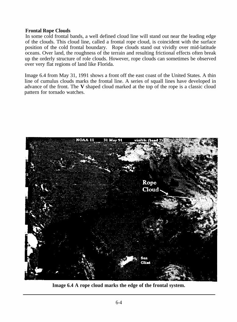
Frontal Rope CloudsIn some cold frontal bands, a well defined cloud line will stand out near the leading edgeof the clouds. This cloud line, called a frontal rope cloud, is coincident with the surfaceposition of the cold frontal boundary. Rope clouds stand out vividly over mid-latitudeoceans. Over land, the roughness of the terrain and resulting frictional effects often breakup the orderly structure of role clouds. However, rope clouds can sometimes be observedover very flat regions of land like Florida.

Image 6.4 from May 31, 1991 shows a front off the east coast of the United States. A thinline of cumulus clouds marks the frontal line. A series of squall lines have developed inadvance of the front. The V shaped cloud marked at the top of the rope is a classic cloudpattern for tornado watches.

-

-.

-

Image 6.4 A rope cloud marks the edge of the frontal system.

6-4

Gust FrontsThunder storms are regions of intense updrafts and downdrafts. As the storm begins todissipate, downdrafts flow out the bottom and ahead of the storm. Because of its downwardvertical motion, this air is cooler than the surrounding air and thus forms a mini cold frontin advance of the thunderstorm itself. The leading edge of the cold air that flows from thebottom of a thunderstorm appears in satellite images as an arc shaped line of convectiveclouds sometimes referred to as a gust front. New thunderstorms can develop along gustfronts particularly where two arcs intersect or where there is already some convectiveactivity. Strong turbulence is generally associated with gust fronts. Wind speeds can easilyexceed 20 knots and in some cases have been believed to reach 100 knots.

Image 6.5 Gust fronts form in advance of thunderstorms.

6-5

6.2 Severe Storms

Squall LinesSquall lines are intense lines of thunderstorms that form ahead of fast moving cold fronts.The squall line forms due to rapidly converging air ahead of a cold front that leads to severethunderstorm and tornado activity. Some squall lines are several hundred miles in length.Squall lines are very prominent weather features, and can be seen on visible (Meteor andband 2) satellite imagery. However, the best analysis tool for tracking squall lines is anenhanced infrared image because vertical development can easily be monitored.

An example of squall lines is shown in APT Image 6.6 captured on January 17, 1991. Acold front off the east coast of the United States is marked by a thin rope cloud. A seriesof squall lines has developed in advance of the front. The V shaped cloud marked at thetop of the rope is a classic cloud pattern for tornado watches.

Image 6.6 Squall lines form in advance of fronts.

6-6

TornadoesTornadoes result from extremelysevere thunderstorm activity.Well developed squall lines andhighly organized cold frontalsystems are prime candidates forthe development of tornadoes.Once you have observed a welldeveloped squall line in visualimagery, you should then switchto thermal imagery to analyzethe detailed cloud structure.

There is a classic V shaped cloudpattern associated with tornadoactivity. This V pattern, ortriangular cloud mass, actuallyresembles a tornado as whenviewed from a satellite’s vantagepoint. Infrared imagery in mostcases will show upper leveldivergence. By tracking themovement of the coldest cloudsthe situation can be monitoredand areas of suspected tornadoactivity can be outlined. Upperlevel divergence is usuallyaccompanied by low levelconvergence resulting in strongupdrafts that accompany severeturbulence, icing, and windysurface gusts.

Images 6.7 and 6.8, captured onMarch 1, 1991 are from theafternoon pass of NOAA 11.The area of potentially severeweather near New Orleans ismarked on the infrared view.Heavy thundershowers werereported in the area but notornadoes were sighted.

Image 6.7 Visible image of storm system.

Image 6.8 Infrared image of storm.

6-7

Thunderstorm Detection and ForecastingMeteorologists forecast weather on severaltime and spatial scales. Clues about theweather over a region on a scale of one tothree days can be derived from watchingfor changes in the amplitude of upper levelair flow. A change from zonal tomeridional flow indicates that more mixingof different air masses is likely. The fullcycle from zonal to meridional back tozonal flow can take 7 to 10 days. If upperlevel divergence is strong, a strong surfacelow will develop to the east of the upperlevel trough. This area should be watchedfor thunderstorm development. Anillustration of the life cycle of a storm isshown here. The life cycle of a cyclonestorm is usually about 3 days.

Life Cycle of a Frontal Wave

(4

(4

Thunderstorm activity is both detectiblean predictable on much smaller timeand space scales. One short term clueis to look for an arc of cumulus cloudsmarking a line of convective activity inadvance of a cold front. Where thesearcs cross each other or where there isstrong convective activity, thunderstormdevelopment is likely.

Thunderstorm intensity can beestimated by monitoring cloud toptemperatures. Cloud tops withtemperatures colder than -55° C aremost likely to be producing intensethunderstorms. One simple trick thatmeteorologists use to visually notewhich clouds are the coldest is toenhance the image coloring all pixels ina low temperature range, for examplefrom -55° C to -60° C, black. Theimages showing cumulonimbus clouds inUnit 4 were enhanced in this way.

Image 6.9 Cold front with thunderstorm activity.

6-8

6.3 Tropical Storms

Image 6.10 Tropical storm Lili at about 3 p.m. on October 11, 1991.

A tropical storm begins as a tropical disturbance, which is a large low pressure area overwarm tropical ocean. If conditions are favorable, an organized pattern of clouds, wind, andrain develops. The first pattern that can be recognized in a satellite image is called atropical depression. Tropical depressions have closed rotary flow at the surface with windsless than 34 knots. When winds increase above 34 knots, the cyclone is classified as atropical storm. When Image 6.10 was captured, Tropical Storm Lili had formed off thecoast of Florida.

Tropical storms are more likely to occur in the summer and autumn than during the rest ofthe year because the three ingredients required to initiate a tropical storm are most likelyto occur at the same time and place during the late summer and autumn. They are:

(1) warm moist converging air,(2) warm ocean, and(3) latitude away from the equator where the Coriolis force caused by the earth’s

rotation is strong enough to increase to potential for cyclone development.

6-9

Image 6.11 Infrared view of tropical storm Lili.

Tropical storms and hurricanes exhibit a great variety of cloud patterns, but most can bedescribed as having a “comma” shape. As the storm develops, the clouds form bands thatwrap around into a center, producing a circular cloud system that often has a cloud-free,dark eye. The number and width of the bands, the solidness of the central dense overcast,and the presence of an eye all enter into the daily assessment of a storm. This closeupinfrared view of Tropical Storm Lili shows a comma shape pattern, a dense center but noeye.

Low level winds near the surface of the ocean, shown as solid arrows, flow in acounterclockwise direction into the center of the storm. Winds emerging out of the top ofthe storm in the upper atmosphere flow in a clockwise direction. Upper level air flow isindicated by double arrows.

Tropical storms begin in the warm converging air of the Inter-Tropical Convergence Zone(ITCZ). They move slowly westward and away from the equator until they reach thesubtropical high pressure zone.the mid-latitude region.

Then, like a slingshot, they accelerate out of the high into

6-10

Image 6.12 Tropical storm Lili late afternoon on October 12, 1991.

This APT image, captured from a NOAA 9 satellite pass on October 12, 1990, shows Liliabout 27 hours after the image on the previous page. Two wide feeders appear to bespiraling into Lily. These feeders can contain intense thunderstorms and tornadoes. Twoweather systems now appear in the image. A Tropical Depression has developed to the eastof Lili.

Lili has grown larger and has moved about 5 degrees to the north and west. Tropical stormsgenerally move at about 10 to 15 miles per hour in the tropics and pick up speed to 30 to50 mph as they move to higher latitudes.

Tropical storms are named alphabetically, each season beginning with “A”. Alternatenames are male and female. How many tropical storms had occurred in 1990 before Lili?

6-11

Image 6.13 By morning on October 13, 1991 tropical storm Lili has burned itself out.

This Automatic Picture Transmission (APT) image was captured from a NOAA 10 satellitepass on October 13, 1990. This is the third day in the evolution of tropical storm Lili. Lilihas nearly burned itself out and is moving to off to the north and east.

Tropical cyclones are classified with respect to their state of development.

Tropical Disturbance: A weak rotary air circulation 160 to 300 kilometers (100 - 300miles) across.Tropical Depression: A closed rotary flow at the surface with wind less than 34 knots(39 mph).Tropical Storm: A closed rotary flow with winds of 34 to 63 knots (75 mph).Hurricane: A warm core tropical storm with wind in excess of 64 knots (75 mph).

Activity: Discuss possible reasons why Lili did not develop into a hurricane.

6-12

Image 6.14 Hurricane Bertha on 31 July, 1991.

When the winds within a tropical storm exceed 64 knots, it becomes a Hurricane. This APTimage, captured from a NOAA 11 satellite pass on July 31, 1990 shows Hurricane Bertha.Both visible and the infrared channels are displayed side-by-side.

Hurricane Bertha has the classic comma shape with two feeders. From the cloud patternsit can be seen that the wind is swirling in a counter clockwise direction near the surface anda clockwise direction out of the top of the system. Heavy rain and high wind was reportedon this day all along the coast of Maine.

Although North Atlantic tropical storms are called hurricanes, in the Pacific, they are calledtyphoons. In the Southern Hemisphere, storms similar to hurricanes and typhoons affectAustralia and Africa as well as many islands such as Madagascar. These are called cyclones.A nickname of “Willy-Willy has been used to refer to hurricanes in Australia.

6-13

Image 6.15 Close up view of hurricane Bertha in the visible band.

The wind increases and the pressure decreases toward the center of a hurricane. Thestrongest winds are at a distance of about 6 to 30 miles from the center. The center, calledthe eye, is a region of relative calm about 6 to 12 miles across.

Activity 1: Scale a HurricaneHow big is the eye of Hurricane Bertha? How wide is the hurricane? These lengths canbe estimated by using the latitude and longitude grid to develop a map scale. Mosthurricanes are about 600 to 800 kilometers (400 to 500 miles) wide. Is Hurricane Berthatypical? (Hint: 1 degree latitude is about 100 kilometers.)

6-14

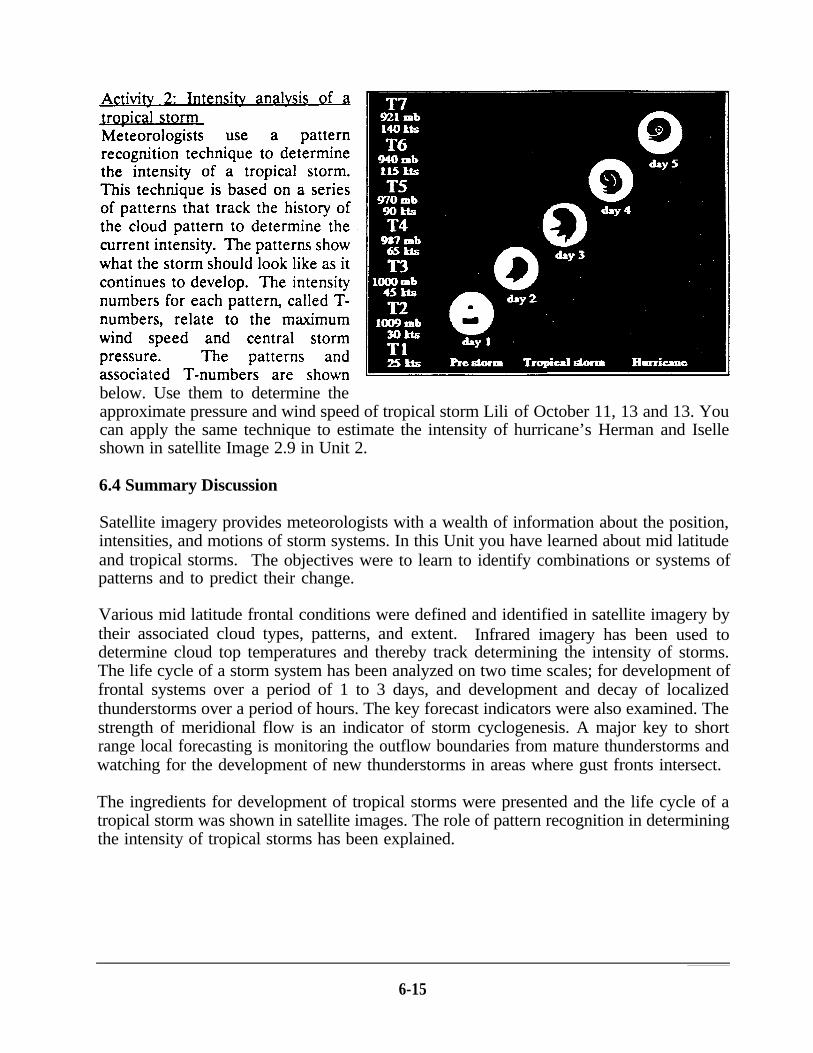
below. Use them to determine theapproximate pressure and wind speed of tropical storm Lilican apply the same technique to estimate the intensity ofshown in satellite Image 2.9 in Unit 2.

6.4 Summary Discussion

of October 11, 13 and 13. Youhurricane’s Herman and Iselle

Satellite imagery provides meteorologists with a wealth of information about the position,intensities, and motions of storm systems. In this Unit you have learned about mid latitudeand tropical storms. The objectives were to learn to identify combinations or systems ofpatterns and to predict their change.

Various mid latitude frontal conditions were defined and identified in satellite imagery bytheir associated cloud types, patterns, and extent. Infrared imagery has been used todetermine cloud top temperatures and thereby track determining the intensity of storms.The life cycle of a storm system has been analyzed on two time scales; for development offrontal systems over a period of 1 to 3 days, and development and decay of localizedthunderstorms over a period of hours. The key forecast indicators were also examined. Thestrength of meridional flow is an indicator of storm cyclogenesis. A major key to shortrange local forecasting is monitoring the outflow boundaries from mature thunderstorms andwatching for the development of new thunderstorms in areas where gust fronts intersect.

The ingredients for development of tropical storms were presented and the life cycle of atropical storm was shown in satellite images. The role of pattern recognition in determiningthe intensity of tropical storms has been explained.

6-15

Unit 7: Applications of Infrared Images to Oceanography

Satellite data are a powerful means for monitoring and forecasting the biological andphysical processes in the world’s oceans. From a polar orbiting satellite’s vantage point theoceans can be mapped every 24 hours. The spatial resolution and area1 extent of a satellitepass are well matched to the physical and biological changes taking place on the oceansurface. The only limitation is cloud cover.

Satellites provide a large scale view of oceans which cannot be obtained with sparsemeasurements from surface vessels. Space and time scales of biological and physicalprocesses in the ocean are compatible with the viewing schedule and resolution of APTimagery. Ocean currents and associated fronts and eddies extend over a range of 10’s to100’s kilometers and move slowly, only a few kilometers each day. Plankton communitiestend to change over periods of one to ten days across an areas extending from 10’s to 100’sof kilometers squared. Even with only nighttime infrared image used, the APT broadcastprovides a minimum of daily coverage at pixel resolution of approximately 4 kilometers.

Clouds are a drawback to using satellite data in some locations. Over the northern ocean’sabove 45 degrees latitude, cloud cover is common more than 70 percent of the time. Insubtropical areas, cloud cover is consistently less than 50 %. Cloud cover in many mid-latitude areas is seasonal. Fishermen and other maritime industries need to be aware ofthese trends. In general however, on any given day about 30 to 40 percent of the world’soceans will be covered by clouds. On average, based on capturing one nighttime infraredimage every twenty four hours, a cloud free image of a 100 km x 100 km area of oceanshould be available every second or third day - sufficiently often to track biological andphysical changes in the ocean as they take place.

7.1 Tracking Ocean Currents

Because both the atmosphere and ocean are large fluid bodies on a rotating earth, it shouldnot be surprising that their large scale flow features have many similar patterns. Oceancurrents move in a clockwise fashion in the Northern Hemisphere and in a counterclockwisefashion in the Southern Hemisphere. Currents on the western side of oceans are channeledand strong as they move away from the equator. Examples include the Gulf Stream alongthe eastern coast of the United States and the Kuroshio Current off the eastern coast ofJapan. On the eastern sides of oceans currents are generally much broader and slower.They tend to move toward the equator and cause upwelling along the western coasts ofcontinents where water is turned away from adjacent land masses.

With the advent of thermal satellite imagery, ships at sea can more accurately account forthe effects of currents on vessel movements. Selecting an optimum route for ships can savemany hours of sailing time and improve safety. In 1975 EXXON and NOAA jointlyconducted a Gulf Stream Navigation Experiment that showed how taking advantage of theGulf Stream flow can result in substantial fuel savings. The western wall of the Gulf Streamis the location of maximum northward current, 2 to 4 knots. Because it has a substantial

7-1

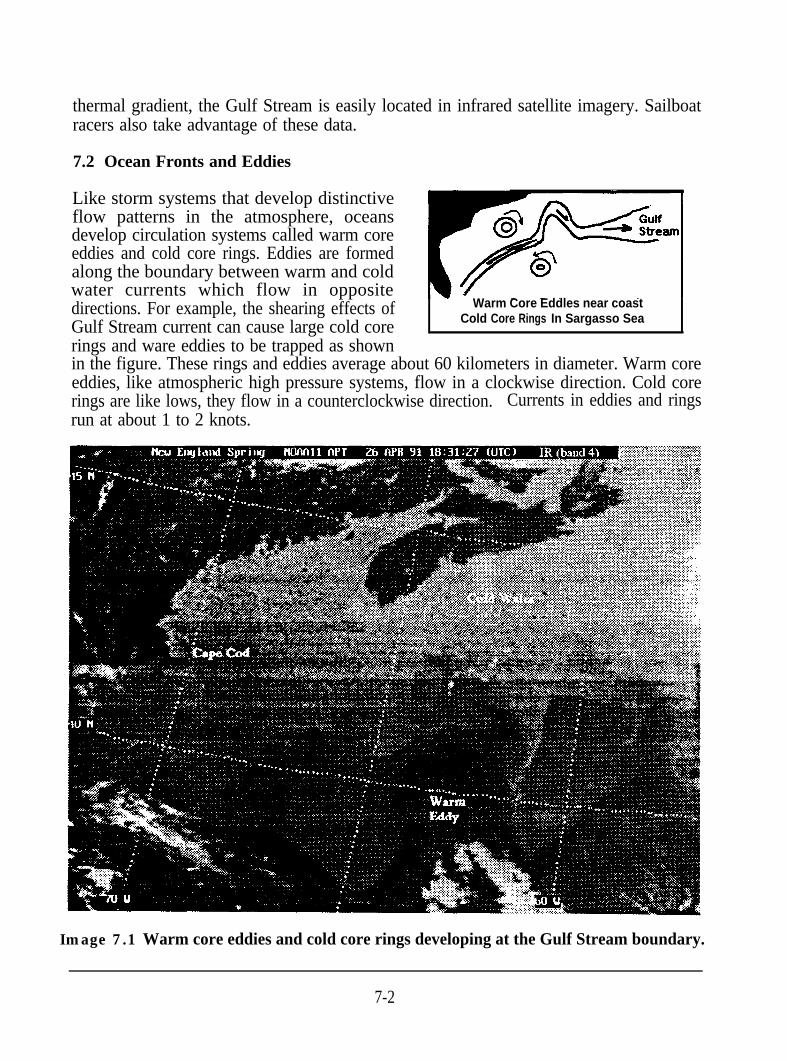
thermal gradient, the Gulf Stream is easily located in infrared satellite imagery. Sailboatracers also take advantage of these data.

7.2 Ocean Fronts and Eddies

Like storm systems that develop distinctiveflow patterns in the atmosphere, oceansdevelop circulation systems called warm coreeddies and cold core rings. Eddies are formedalong the boundary between warm and coldwater currents which flow in opposite

r#-4Ljm

directions. For example, the shearing effects of Warm Core Eddles near coast

Gulf Stream current can cause large cold core Cold Core Rings In Sargasso Sea

rings and ware eddies to be trapped as shownin the figure. These rings and eddies average about 60 kilometers in diameter. Warm coreeddies, like atmospheric high pressure systems, flow in a clockwise direction. Cold corerings are like lows, they flow in a counterclockwise direction. Currents in eddies and ringsrun at about 1 to 2 knots.

Image 7.1 Warm core eddies and cold core rings developing at the Gulf Stream boundary.

7-2

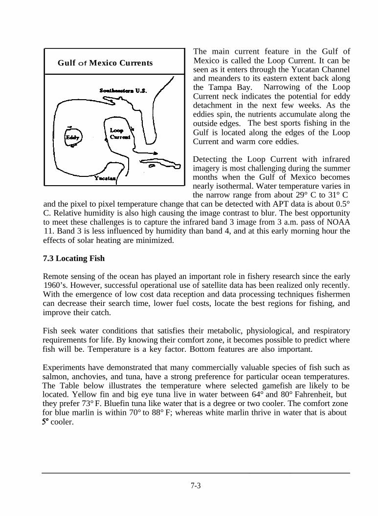
Gulf of Mexico CurrentsThe main current feature in the Gulf ofMexico is called the Loop Current. It can beseen as it enters through the Yucatan Channeland meanders to its eastern extent back alongthe Tampa Bay. Narrowing of the LoopCurrent neck indicates the potential for eddydetachment in the next few weeks. As theeddies spin, the nutrients accumulate along theoutside edges. The best sports fishing in theGulf is located along the edges of the LoopCurrent and warm core eddies.

Detecting the Loop Current with infraredimagery is most challenging during the summermonths when the Gulf of Mexico becomesnearly isothermal. Water temperature varies inthe narrow range from about 29° C to 31° C

and the pixel to pixel temperature change that can be detected with APT data is about 0.5°C. Relative humidity is also high causing the image contrast to blur. The best opportunityto meet these challenges is to capture the infrared band 3 image from 3 a.m. pass of NOAA11. Band 3 is less influenced by humidity than band 4, and at this early morning hour theeffects of solar heating are minimized.

7.3 Locating Fish

Remote sensing of the ocean has played an important role in fishery research since the early1960’s. However, successful operational use of satellite data has been realized only recently.With the emergence of low cost data reception and data processing techniques fishermencan decrease their search time, lower fuel costs, locate the best regions for fishing, andimprove their catch.

Fish seek water conditions that satisfies their metabolic, physiological, and respiratoryrequirements for life. By knowing their comfort zone, it becomes possible to predict wherefish will be. Temperature is a key factor. Bottom features are also important.

Experiments have demonstrated that many commercially valuable species of fish such assalmon, anchovies, and tuna, have a strong preference for particular ocean temperatures.The Table below illustrates the temperature where selected gamefish are likely to belocated. Yellow fin and big eye tuna live in water between 64° and 80° Fahrenheit, but

they prefer 73° F. Bluefin tuna like water that is a degree or two cooler. The comfort zonefor blue marlin is within 70° to 88° F; whereas white marlin thrive in water that is about5” cooler.

7-3

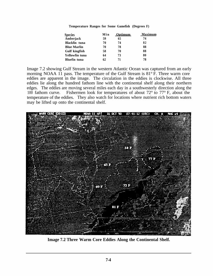
Temperature Ranges for Some Gamefish (Degrees F)

Species M i n Optimum MaximumAmberjack 59 65 74Blackfin tuna 70 74 8 2Blue Marlin 70 78 88Gulf kingfish 58 70 88Yellowfin tuna 64 73 80Bluefin tuna 62 71 78

Image 7.2 showing Gulf Stream in the western Atlantic Ocean was captured from an earlymorning NOAA 11 pass. The temperature of the Gulf Stream is 81° F. Three warm coreeddies are apparent in the image. The circulation in the eddies is clockwise. All threeeddies lie along the hundred fathom line with the continental shelf along their northernedges. The eddies are moving several miles each day in a southwesterly direction along the100 fathom curve. Fishermen look for temperatures of about 72° to 77° F, about thetemperature of the eddies. They also watch for locations where nutrient rich bottom watersmay be lifted up onto the continental shelf.

Image 7.2 Three Warm Core Eddies Along the Continental Shelf.

7-4

Water temperature can also be used to find theareas where fish are eating or spawning.Areas of vertical upwelling, of deep coldnutrient-rich water can easily detected withinfrared imagery. These nutrients, whencombined with available sunlight near theocean’s surface, cause an increase in planktongrowth and thus mark areas for fish feedingand spawning. Upwelling areas tend to behighly productive and are often the site ofimportant fisheries, such as the anchovy fisheryoff the coast of California. Upwelling is largely

caused by wind stress and occurs off the west coast of continents. Winds favorable toupwelling vary on a time scale of 3 to 5 days. Upwelling can also be caused by the bottomtopography as illustrated in the picture to the left.

Upwelling and its effects on food production have been related to the survival of juvenilesalmon after they leave the Columbia River and enter the Pacific. The young salmon tendto stay within 28 kilometers from shore in the narrow belt of the river’s plume. However,they count on nutrients from upwelling coastal waters for food production.

7.4 Summary and Discussion

Thermal infrared imagery is used to locate fish populations, trace ocean current boundaries,optimize ship routes, and support other maritime activities. Sea-surface temperature datafrom satellite infrared imagery are used to prepare eddy forecasts for offshore oilexploration and production. Temporal changes in eddy size and position and current frontallocations are used to produce routine summaries of eddy positions and the direction ofsurface currents. Temperature maps can also be used to estimate the global uptake ofcarbon dioxide, the primary greenhouse gas, by ocean biomass. The productivity of ouroceans and coastal environment is a major environmental concern for the 1990’s. Marineplankton biomass accounts for at least 30 percent of the total global annual plant storageof carbon dioxide.

You class may want to select one of the following research topics for further study anddiscussion. How does the temperature of ocean waters effect cloud formation?Hypothesize and test how currents at the surface of the ocean compare with bottomcontours? What are the advantages of knowing the location of the Gulf Stream?

Global Change research is now focusing on anomalous warm ocean conditions in the Pacificcalled El Nino events. These events appear to reduce upwelling along the western coast ofthe United States. Based on this observation, you might hypothesize how an El Nino eventwould effect plankton productivity. What would be the possible feedbacks to carbon dioxidestorage in the ocean? You can test your hypothesis by collecting, logging, and mapping thechange in ocean temperature over the school year.

7-5

-

Unit 8: Applications of Visible Images to Agriculture

This unit examines the role of APT satellite weather data in agricultural applications. Theskills learned in earlier units will be applied to interpreting selected APT images capturedduring the fall and winter growing season of a winter wheat producing area in the PacificNorthwest. The region is diverse in terrain, soil characteristics, and vegetation providing aninteresting opportunity to test your image interpretation skills. The objective is tofamiliarize you with agricultural issues while providing an opportunity to characterizesatellite imagery in the visible and infrared spectrum. This unit will assist you in becomingfamiliar with mapping and charting. You will distinguish snow cover from clouds andappreciate the importance of orographic lifting to producing precipitation along mountainslopes. This unit illustrates to educators and students the importance of timely weather andremote sensing data to the farming community.

8.1 Timing of Tillage and Field Operations

The use of APT signal reception and imaging from polar orbiting satellites when used inconjunction with WEFAX signal from geostationary satellites allows tracking storm frontsand other significant weather systems. An estimate of the relative intensity of weathersystems can be made by monitoring the temperature of the cloud tops. This type ofinformation is useful for scheduling the timing of tillage and other field operations.

Initial spring tillage operations for dryland small grain production in the inland Northwestare ideally begun when soils have drained and firmed enough to minimize compaction fromtillage equipment. Soil temperatures should be warm enough to promote germination ofplanted seeds and the development of a healthy seedling. If initial tillage of over-winteredplowed ground is followed by heavy rains, soils high in clay content will retain that moistureand dry more slowly than if tillage had not occurred. This is due to a relative loss ofporosity of the soil mass because larger air pockets created by plowing the previous fall areeliminated by the initial spring tillage. The rough, domed ridges left by plowing are alsoreduced, producing a finer more uniform soil surface. The total surface area exposed to theair is also reduced, thus reducing the capacity for evaporative drying. The timely delay ofthe initial tillage until after passage of an impending heavy or prolonged rain can ultimatelylead to an overall quicker sequence of tillage operations in preparing the seed bed forplanting.

8.2 Herbicide Selection and Timing of Application

Decisions based on recent past and near term future weather conditions contribute to themost economical and environmentally safe use of herbicides used to suppress or eliminatenoxious weeds in agricultural fields. Both the crop under cultivation and the herbicidechosen for use on that crop can be sensitive to and respond to changes in weather conditionsfollowing the period of application. Extremes of cloudiness (as it affects incoming solarradiation and the resulting level of photosynthetic activity within a plant), temperature,

8-l

8.1 Infrared image of a storm effecting herbicide application.

rainfall, individually and collectively, influence the activity of the herbicide and the responseof weeds and the desired crop to that activity. By tracking weather systems which may poseproblems or offer specific benefits to the use of certain selective herbicides, it is possible toalter the timing of application or lessen the concentration of product used. For example,NOAA infrared Image 8.1 depicts a storm affecting the interior West and Northwest on May19, 1991. The center of low pressure is over Nevada and backwash from the counter-clockwise circulation is moving from Montana through Idaho into the Palouse region ofeastern Washington. On May 17 a pre-emergent herbicide application for broadleaf weedcontrol was needed in a seeded field near the Washington-Idaho border. Crop emergencewas one to two days away. The storm had been tracked for several days prior to theapplication date. Based on the intensity of the system as estimated by measuring cloud toptemperatures and the general direction of movement, significant rainfall appeared imminent.Because the particular herbicide being applied relies on rainfall to carry it into the rootzone of germinating weed seeds and excessive rainfall can carry the product deeper in tothe zone of germinating crop seed with the potential for crop damage, a 20 percentreduction in the concentration of product used was made at the time of application. Theimage shows the storm in the middle of delivering a two day rainfall total of .82 inches asrecorded near the application site. This is about 60 percent more rain than necessary toproperly place the herbicide within the zone of germinating weeds. To date weed control

8-2

has been excellent and there is no evidence of crop damage. Results of the application willcontinue to be monitored and used in future decision making.

Apart from rate reductions as in the previous example, if a choice of herbicides is available,it may be possible to select a different herbicide which will more closely fit the expectedweather condition. In some instances, given impending severe weather conditions, it maybe necessary to forgo the application altogether for the sake of crop safety.

8.3 Timing of Additional Field Operations

In the later phases of the production cycle certain crops, such as alfalfa, hay, grass hay andpulses (lentils, dry peas etc.) are mowed or swathed into rows and a period of warm, dryweather is needed for the crop to cure and achieve proper moisture content. This precedesbaling in the case of hay or harvesting in the case of pulses. A prolonged period ofsustained rains after swathing interrupts the drying process and can cause substantialeconomic losses from a degradation of crop quality or from spoilage due to the growth ofmicroorganisms such as fungi. Delaying the swathing process to avoid damage fromapproaching excessive rainfall or high winds is clearly advantageous.

8.4 Winter Wheat Season in the Palouse

The Palouse, in Whitman County of eastern Washington is famous for dryland farming,particularly the production of lentils and winter wheat. Farmers of the Palouse routinelyaverage 60 to 80 bushels of wheat per acre. In years with favorable weather conditionsthroughout the growing season, areas of the Palouse will average 90 to 100 bushels per acre.

The Palouse, which spans the Washington-Idaho border and lies about 200 miles fromWashington’s Mount St. Helens, is unusual not only for its agricultural productivity, butbecause its rolling terrain is rugged for farming. Hilltops in the Palouse, unlike thewindswept hills of the midwestem prairies, are still relatively productive. Soil erosion fromexcessive rains is a problem, but farmers and equipment engineers continue to develop newfarming practices and design new machinery to protect that vital resource.

The winter wheat crop is usually planted in September and early October for harvest thefollowing summer. Fall rains are responsible for germinating planted seeds on annuallycropped ground. Many farmers regard management of this moisture as a necessary firststep in establishing a healthy stand of wheat. Following emergence, the wheat’s root systemcontinues to develop and the plant should reach the three to four leaf stage before coldtemperatures of late fall and early winter harden the plant and lead it to a state ofdormancy.

As we track the weather from planting of winter wheat in September until early spring, wewill track the health of the crop as reported in the Weekly Weather and Crop Bulletin for thesame time period. This publication is produced jointly by the U.S. Department ofCommerce and the Department of Agriculture. Each issue begins with a short, general

8-3

description of major weather patterns for the nation, then follows with a one paragraphsummary of agricultural activities for each state. The agricultural community subscribes tothis publication because it gives them a look at general weather conditions in agriculturalregions world wide which produce the same crops and thus compete in world markets. Forexample, Australia raises the same type of wheat (soft white) as farmers in the PacificNorthwest and is therefore a competitor for sales in the Middle East and Southeast Asianmarkets. Although publications like the Weekly Weather and Crop Bulletin are valuablepublications, they are not timely. They are usually received several weeks and sometimesup to a month after the fact. Farmers cannot rely on information which is basicallyhistorical for time sensitive decisions. This is an area where satellite delivery of images andinformation really helps out.

The following series of Soviet Meteor images illustrates how snow cover can be monitoredin a general way in mountains or in areas of agricultural production. Farmers depend onadequate snow cover to insulate fall seeded wheat and barley plants which have emergedand are vulnerable to damage or winter kill by cold arctic air. The developing crop isespecially at risk when strong winds also accompany low temperatures. In addition tocausing sever dehydration, fine soil particles and ice crystals can be blown so swiftly alongthe ground that exposed leaves can be shredded or cut off at the crown of the plant.

8-4

September:Early September through mid-October mark the planting season for winter wheat in easternWashington. In early September the weather is suitable for fieldwork as illustrated in thisSeptember 13, 1990 Meteor pass which covers an area from south central California toBritish Columbia. A high pressure system persists over the west and clouds cover the northcoastal area of the Olympic Peninsula of Washington State. Mounts Olympus, Baker,Rainier, Adams, Hood, Shasta, Lassen and ash laden areas around Mt. St. Helens are visibleas white dots on the image attributable to clouds covering their peaks. If you examine thisimage closely, you should be able to find numerous lakes including Lake Banks, LakeRoosevelt, and the Potholes Reservoir in Washington. It is also possible to discern PendOrielle and Coeur d ‘Alene nestled in forested areas of Oregon. Further examination ofthe image reveals Utah’s Great Salt Lake and California’s Tahoe, Mono, and Goose lakesand the Snake and Columbia Rivers. Old growth timber of the Olympic National Forestis distinct as well as the channeled scablands of central Washington.

The lighter areas of the image, between the Columbia River and the Blue Mountains ofsoutheastern Washington, are harvested croplands. Harvested areas are also apparent northand east of the Snake River eastward to the foothills of the Clearwater Mountains. This isthe Palouse region. Agricultural regions of the Willamette Valley in Oregon also appearlighter as do British Columbia’s Okanogan and Frazier Valleys.

October:By October the winter wheat has emerged in the Palouse. The Weekly Weather and CropBulletin for October 23rd indicates that the crop is in good to fair condition across the area.Based on favorable weather conditions, the crop is off to a fine start. This image, capturedon October 14th shows overcast conditions. Precipitation measured about .68 inches in nearTekoa in the Palouse. The first snowfall can usually be expected around the end ofOctober.

-

-

-

Image 8.3 Rain after planting starts the crop off right.

8-6

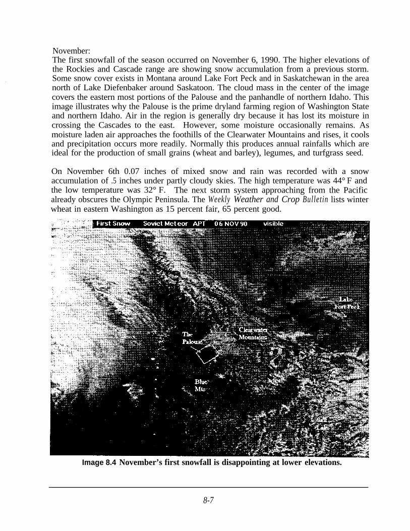
November:The first snowfall of the season occurred on November 6, 1990. The higher elevations ofthe Rockies and Cascade range are showing snow accumulation from a previous storm.Some snow cover exists in Montana around Lake Fort Peck and in Saskatchewan in the areanorth of Lake Diefenbaker around Saskatoon. The cloud mass in the center of the imagecovers the eastern most portions of the Palouse and the panhandle of northern Idaho. Thisimage illustrates why the Palouse is the prime dryland farming region of Washington Stateand northern Idaho. Air in the region is generally dry because it has lost its moisture incrossing the Cascades to the east. However, some moisture occasionally remains. Asmoisture laden air approaches the foothills of the Clearwater Mountains and rises, it coolsand precipitation occurs more readily. Normally this produces annual rainfalls which areideal for the production of small grains (wheat and barley), legumes, and turfgrass seed.

On November 6th 0.07 inches of mixed snow and rain was recorded with a snowaccumulation of .5 inches under partly cloudy skies. The high temperature was 44° F andthe low temperature was 32° F. The next storm system approaching from the Pacificalready obscures the Olympic Peninsula. The Weekly Weather and Crop Bulletin lists winterwheat in eastern Washington as 15 percent fair, 65 percent good.

Image 8.4 November’s first snowfall is disappointing at lower elevations.

8-7

-

The November image reveals how scant snow cover was in the Palouse region of easternWashington at that time. Good protective ground cover is not observed until we examinethe areas around Dayton and Walla Walla in southeastern Washington. Basically this heldtrue until December when depicts arctic air moved into the area from a high pressuresystem over Canada to a low pressure center in southern Oregon.

December:On December 19, 1990 a high pressure system was over western Canada and a low pressuresystem centered over coastal southern Oregon. These are conditions which farmers in thePalouse dread because they cause a frigid air mass to move quickly into the area from thenortheast. Winds associated with this air mass are usually strong. Temperature extremesdropped from high a high of 42° F and a low of 30° F on December 17th to a high of 8° 30 F on December 17th to a high of 8”F and a low of -2° F on the 19th. Only a trace of snow is recorded leaving most areas ofwinter wheat exposed to punishing conditions. The depth of frozen soil fell from 4 cm onDecember 17 th to 40.8 cm on December 25th.

8-8

Just west of the Blue Mountains around Dayton and Walla Walla a heavier amount of snowaccumulated providing an insulation layer over the wheat. Overall, though, this stormproved to be very damaging to the developing crop. The Weekly Weather and Crop Bulletinof December 16-22 rated Washington winter wheat crop 72 percent good and 8 percent poorto very poor. In January the bulletin reported " Winter wheat has been damaged by strongwinds, extreme cold temperature in central, eastern areas.” By the end of January thewinter wheat crop was rated as 32 percent fair, 60 percent poor, and 8 percent very poor.By February, 58 percent of the winter wheat crop was rated as in very poor condition.

By tracking snow cover in agricultural regions as was done in these APT images, farmersand seed supply companies can monitor how widespread an area is susceptible to damagefrom arctic air masses if snow cover is not present. This information can serve as an earlywarning to growers and gives them an opportunity to insure adequate supplies of springwheat varieties are reserved in case widespread reseeding of winter killed areas is required.

The same arctic front that damaged the winter wheat crop of northeastern Washington, wasalso responsible for widespread damage to fruit trees in California’s San Joaquin andImperial Valleys during the winter of 1990.

8-9

Glossary of Terms and Acronyms

Adiabatic - A thermodynamic process that takes place without external exchange of heat.

Advection - Process of heating or cooling an air mass by transporting it horizontally over anobject of different temperature.

Amplitude - Size of the vertical displacement produced by a wave.

APT - Automatic Picture Transmission. Term for the lowbroadcast.

AVHRR - Advanced Very High Resolution Radiometer. TheNOAA’s TIROS-N satellite series.

data rate satellite weather

name of the instrument on

Black Body - A perfect absorber and emitter of radiation. An object that emits an amountof radiation equal to the amount it absorbs.

Brightness - Radiated energy flux entering the satellite sensor’s field of view from an objectbeneath. The direction of radiation differentiates brightness from radiance. Incomingradiation is brightness.

Convection - Process of heat transfer through vertical motion caused by unequal heating ofthe atmosphere.

Dendritic Pattern - A tree or branch-like pattern of snow as imaged from a satellite.

Dew Point Temperature - The temperature to which air must be cooled to reach saturation.

Electromagnetic Radiation - Energy transmitted through space in the form of electric andmagnetic wave fields.

Electromagnetic Spectrum -function of wavelength.

The ordered arrangement of electromagnetic radiation as a

Emissivity - The ratio of the observed brightness of an object to the ideal brightness if itwere a black body.

Frequency - The number of waves passing a given point per unit time.

Front - The boundary zone between two air masses with different properties.

Gust Front - Arc shaped line of convective clouds ahead of a mature thunderstorm causedby downdrafts out the bottom of the storm.

-

-

-

A - l

Histogram - A statistical representation of a digital image showing the number of greyshades and the frequency of occurrence of each shade.

Hurricane - A warm core tropical storm with winds in excess of 64 knots.

ITCZ - Intertropicalequator.

Convergence Zone. A permanent belt of low pressure around the

Jet Stream - A belt of strong westerly winds aloft. The height of the jet stream is typicallybetween 10 to 12 kilometers (6.2 to 7.5 miles).

Latent Heat - The heat released or absorbed by a substance when it changes state.

Latitude - Distance on the Earth’s surface measured in degrees north and south of theequator.

Longitude - Distance on the Earth’s surface measured in degrees east and west from theprime meridian.

Meridional Flow - A condition when the amplitudeconducive to mixing of cold and warm air masses.

of upper level flow is large and

Nadir View - A view directly down from the satellite to the earth at its closest point. Thispoint will be along a line from the satellite to the center of Earth.

NOAA - National Oceanic and Atmospheric Administration. A division of the Departmentof Commerce that operates the National Weather Service and the National EnvironmentalSatellite Data and Information Service.

Optical Thicknessatmosphere.

Orographic Lifting

The collective effects of scattering and absorption of light in the

Lifting of an air mass as it is transported over mountains.

Pixel - picture element. The smallest resolvable unit of an image. The fundamental buildingblock of a digital image.

Radiance - Energy flux leaving a unit area into a cone shaped solid angle defined by thesatellite sensor field of view. The direction of radiation differentiates radiance frombrightness. Radiance is outgoing energy from an object.

Radiometer - An instrument that measures radiation brightness within a fixed band ofwavelengths.

A - 2

Reflectance - The ratio of the energy flux reflected from an object to the energy incident onit. If the reflectance = 1, then one energy is transmitted or absorbed by the object,

Remote Sensing - A method of measuring properties of objects without making physicalcontact.

Ridge - A region of upward displacement of a wave. In meteorology, the location ofmaximum clockwise curvature on an atmospheric wave.

Saturation - When evaporation equals condensation.

Spectral Signature - The reflectance, absorbance and transmittance of an object.

Stretching - Enhancing the contrast of an image over a selected range of pixel values.

Trade winds -A consistent easterly wind in the tropics. North of the equator the trades arefrom the northeast. South of the equator they are from the southeast. Trade winds are amajor component of the atmosphere’s general circulation.

Transmittance - The probability that light reflected or emitted from the earth’s surface willarrive at the satellite. The probability that light will be transmitted through the atmosphere.

Thermodynamics - The study of the solid, liquid, and gaseous states of a system.

Transverse Bands - Cloud bands perpendicular to the air flow that are associated withturbulent wind shear along the jet stream.

Tropical Depression - Closed rotary flow around a low pressure area over the tropicalocean. Winds less than 34 knots.

Tropical Disturbance - Weak rotary air circulation 160 to 300 kilometers across associatedwith a low pressure area over the tropical ocean.

Tropical Storm - A closed rotary flow around a low pressure system over warm tropicalocean. Winds of 34 to 63 knots.

Troposphere - The lowest portion of the atmosphere characterized by decreasingtemperature with altitude - usually about 15 kilometers (9.5 miles) deep. The layer in whichall weather takes place.

Trough - A region-of downward displacement of a wave. In meteorology, the location onan upper level wave where the wind shifts from the northwest to the southwest.

Wave - A massless pattern that moves with regular oscillations.

A - 3

- Wavelength - The interval at which a wave pattern repeats itself. Can be measured frompeak to peak or trough to trough.

Westerlies - A consistent wind from the west occurring in the mid-latitudes. A majorcomponent of the general circulation of the atmosphere.

Zonal Flow - A condition when the amplitude of the upper level flow is small.

A - 4