REFERENCE

Alfredo H-S. Ang and Wilson H. Tang, "Probability Concepts in Engineering Planning andDesign, Volume II � Decision, Risk, and Reliability."

Allan, R.J.:"Integrated Motion, Stability and Variable Load Design of the TrendsetterClass Semisubmersible 'Zane Barnes'".Offshore Technology Conference, Texas, May 2-51988. OTC 5625.

American Petroleum Institute, 1991. "Recommnded Practice for Design, Analysis, andMaintance of Mooring for Floating Production Systems. API Recommended Practice2FP1 RP 2FP1!. First Edition. Washington, D.C..

American Petroleum Institute, 1993. "Recommended Practice for Planning, Designing andConstructing Fixed Offshore Platforms - Load and Resistance Factor Design RP 2A-LRFD!." First Edition, July, Washington, D.C.

American Petroleum Insititute �994!. Recommended Practice for Design and Analysis ofStationkeeping System for Floating Structures. Washington, D.C..

Atkinson, A. C.: The Computer Generation of Poisson Random Variables, Appl Statist.,28: 29-35 �979!.

Baker, M.J.:" Structural Reliability Theory and Its Applications". Springer-Verlag, Berlin,Heidelberg, New York, 1982.

Bea, R.G. 1973. "Wave Forces, Comparision of Stokes Fifth and Stream FunctionTheories." Engineering Note No. 40, Environmental Mechanics, April.

Bea, R.G.:"Gulf of Mexico Hurricane Wave Heights". Journal af Petroleum Technologh.September 1975. 1160-1171.

Bea, R.G., Lai, N.W., 1978. "Hydrodynamic Loadings on Offshore Structures."Proceedings, Offshore Technology Conference, OTC No. 3064. Houston, TX.

Bea, R.G.:"Gulf of Mexico Shallow-Water Wave Heights and Forces". OffshoreTechnology Conference, Texas, May 2-5, 1983. OTC4586.

Bea, R.G., Pawsey, S.F., Litton, R.W., 1986. "Measured and Predicted Wave Forces anOffshore Platforms." Proceedings, Offshore Technology Conference, OTC No. 5787.Houston, TX.

175

Bea, R.G.:" Review of Tropical Cyclone Parameters for Goodwyn A PlatformEnvironmental Criteria" Report to Woodside Offshore Petroleum Ltd. Perth, WesternAustralia. February 1989.

Bea, R.G.:" Wind Bc Wave Forces on Marine Structures". CE/NA 2058 Class Notes.Department of Civil Engineering and Department of Naval Architecture 8c OffshoreEngireering, University of California, Berkeley.

Bea, R.G.:"Reliability Based Design Criteria for Coastal and Ocean Structures". Australia,1990.

Bea, R.G., Young, C., 1993. "Loading and Capacity Effects on Platform Performance inExtreme Condition Storm Waves & Earthquakes." ProomHngs, Offshore TechnologyConference, OTC No. 7140. Houston, 17 .

Bea, R.G. and Mortazavi, M., 1995. "Screening Methodologies for Use in PlatformAssessments and Requalifications." Final Report, Department of Civil Engineering,University of California at Berkeley.

Bobba, A.G.; Singh, V.P.; Bengtsson, L., "Application of uncertainty analysis togroundwater pollution modeling". Environmental Geology, v 26 p 89-96, September 95.

Bratley, P., B. L. Fox, and L. E. Schrage: A Guide to Simulation, 2d ed., Spring-Verlag,New York �987!.

Burganos, V. N.; Paraskeva, C. A.; Payatakes, A.C., "Monte Carlo network simulation ofhorizontal, upflow and downflow depth filtration". AIChE Journal, v 41 p 272-85,February 95.

Burke, B.D., "Downtime Evaluation for Operations from Floating Vessel in Waves",SNAME Spring Meeting/STAR Symposium, San Francisco, Calif., May 1977.

Carr, Lester E.; Elsberry, Russell L., "Systematic and integrated approach to tropicalcyclone track forecasting part 1., approach overview and description of meteorologicalbasis". Naval Postgraduate School, Monterey, California.

Chen, Henry; Rawstron, Phil. "Systems Approach to Offshore Construction ProjectPlanning and Scheduling". Marine Technology, v 20, No. 4, Oct. 1983, pp. 332-347.

Chylek, Petr; Dobbie, J. Steven. "Radiative properties of finite inhomogeneous cirrusclouds: Monte Carlo simulations". Journal of the Atmospheric Science. v 52 p 3512-22,October 15, 1995.

Cochran, W.G., "Sampling Techniques", Third Edition, John Wiley, 1977.

176

Cooper, C. K., Parametric Models of Hurricane-Generated Winds, Waves, and Currents inDeep Water. Conoco Inc.

Dean, R.G., 1977. "Hybrid Method of Computing Wave Loading." Proceedings, OffshoreTechnology Conference, OTC 3029, Houston TX, May.

Det Norske Veritas, 1993. '%'AJAC. Wave and Current Loads on Fixed Rigid FrameStructures." DNV SESAM AS. Version 5.4-02,

Draft Recommended Practice for Design, Analysis, and Maintenance of Mooring forHeating Production Systems. API Recornrrended Practice 2FPI RP 2FPl!. First Edition,May 1, 1991.

Elsberry, Russell L.; Frank, William M.; Holland, Greg J.; Jarrell, Jerry D.; Southern,Robert L., "A Global View of Tropical Cyclones". Based largely on materials prepared forthe International Workshop on Tropical Cyclones, Bangkok, Thailand, November 25 toDecember 5, 1985.

Evans, K. Franklin. 'Two-dimensional radiative transfer in cloudy atmospheres: thespherical harmonic spatial grid method".Journal of the Atmospheric Sciences, v 50 p3111-24, September 15, 1993.

Fenton, J.D., 1985. "A Fifth Order Stokes Theory for Steady Waves, "ASCE Journal ofWaterway, Port, Coastal and Ocean Engineering, Vol. 111, No. 2, pp.216-234.

Fishman, G. S.: Estimating Sample Size in Computer Simulation Experiments,Management Sci., 18; 21-38 �971!,

Glynn, P. W.: Stochastic Approximation for Monte Carlo Optimization, Proc. 1986Winter Simulation Conference, Washington, D. C., pp. 356-365 �986!.

Grosenbaugh, L R.: More on Fortran Random Number Generators, Commun. Assoc.Comput. Math., 12: 639 �969!.

Hahn, G. J., and S. S. Shapiro: Statistical Models in Engineering, John Wiley, New York�967!.-

Hammersley, J. M., and D. C. Handscomb: Monte Carlo Methods, Methuen, London�964!.

Haring, R.E., and Heideman, J.C. �980!. "Gulf of Mexico Rare Return Periods", Journalof Petroleum Technology, Society of Petroleum Engineers, Dallas, TX.

Heidelberger, P.: Variance Reduction Techniques for the Simulation of Markov Processes,I: Multiple Estimates, IBM J. res. Develop., 24:570-581 �980!.

177

Heideman, J.C., Weaver, T.O., 1992. "Static Wave Force Procedure for PlatformDesign." Proceedings of Civil Engineering in the Oceans V, College Station, Texas,American Society of Civil Engineers, New York.

Hindcast Study of Hurricane Andrew �992!, Offshore Gulf of Mexico. OceanweatherInc.Cos Cob, ct. November 1992.

Hoffman, D. and Fitzgerakl, V., "System Approach to Offshore Crane Ship Operations",Trans. SNAME, Vol 86, 1978.

Hu, Sau-Lon Janes; Gupta, Manish; Zhao, Dongshen. "Effects of waveintermittency/nonlinearity on forces and responses". Journal of Engineering Mechanics. v121 p 819-27, July 95.

Law, Averili M.; Keiton, W.David, Simulation Modeling and Analysis". Second edition,McGraw-Hill Series in Industrial Engineering and Management Science.

L'Ecuyer, P.: Random Numbers for Simulation, Commun. Assoc. Comput. Mach., 33:�990!.

McCarron, J.K., "Computer Simulation as a Tool for Evaluating Offshore ConstructionAlternatives". OTC Paper 1353, Offshore Technology Conference, Houston, Tex., 1971.

McDonald, D.T., Bando, K., Bea, R.G., Sobey, R.J., 1990. " Near Surface Wave Forceson Horizontal Members and Decks of Offshore Platforms." Final Report, Coastal andHydraulic Engineering, Dept. of Civil Engineering, University of California at Berkeley,Dec.

McDonald, David T., "Reliability Evaluation of a Jack-up Drilling Unit in the North Seaand in the Gulf of Mexico." MS Thesis, Department of Civil Engineering, University ofCalifornia, Berkeley.

Mehrdad Mortazavi, "A Probabilistic Screening Methodology for Use in Assessment andRequalification of Steel, Template- Type Offshore Platforms". Ph.D Dissertation,Department of Civil Engineering, University of California at Berkeley.

Moore, W.H., 1993. "Management of Human and Organizational Error in Operations ofmarine Systems." Ph.D Dissertation, Graduate Division, Univ. of Cal. at Berkeley.

Morison, J.R., O' Brien, M.P., Johnson, J.W., Schaff, S.A., 1950. 'The Force Exerted bySurface Waves on Piles." Petrol. Trans. AIME, Vol. 189, pp 149-154.

Naghavi, Babak; Yu, Fang Xin. "Regional &equency analysis of extreme precipitation inLouisiana". Journal of Hydraulic Engineering, v 121, p 819-27, November 95.

17S

Noble Denton, 1991. "Climate of Environmental Extremes Tropical Storm Areas", FinalReport. Report No., L14839/NDWS/HDL

Oceanweather Inc. �992!. Hindcast Study of Hurricane Andrew - OfFshore Gulf ofMexico. Cos Cob, Cl.

Oppenlander, Joseph C.; Oppenlander, Jane E., "Storage lengths for left-turn lanes withseparate phase control". ITE Journal, v 64 p 22-6, January 94.

Petrauskas, C., Botelho, D.LR., Krieger, W.F., and GriKn, J.J., 1994. "A ReliabiTityModel for Offshore Platforms and its Application to ST 151 H and K Platforms DuringHurricane Andrew �992!." Proceedings of the Behavior of OfFshore Structure Systems,Boss '94, Massachusetts Institute of Technology.

Petrauskas, C., Heideman, J.C., Berek, E.P., 1993. "Extreme Wave-Force CalculationProcedure for the 20th Edition of API RP-2A." Proceedings, Offshore TechnologyConference, OTC 7153, Houston, Texas, May.

Petrauskas, C., Heideman, J.C., and Berek, E.P., 1993. Extreme Wave Force CalculationProcedure for 20th Edition of API RP 2A." Proceedings, Offshore TechnologyConference, OTC 7153, Houston, TX.

Praught, M and Devlin, P., "Evaluating OfFshore Construction Activities Using a ProjectSimulation Program". SNAME, Northern California, Section, Nov. 1982.

Preston, D., 1994, "An Assessment of the Environmental Loads on the Ocean MotionInternational Platform," MS Thesis, Department of Naval Architecture and OffshoreEngineering, University of California, Berkeley, USA.

Pritsker, A. Alan B. and Claude Dennis Pegden, "Introduction to Simulation and SLAM."

Rault, Didier F. G.; Woronowicz, Michael S., "Application of direct simulation MonteCarlo to satellite contamination studies". Journal of Spacecraft and Rockets, v 32 p 392-7May/June 95.

R & B, Gulf of Mexico Hurricane Evacuation Procedures, Zane Barnes, 1988.

Rhee, Seung-Whee; Reible, Danny D.; Constant, W. David. "Stochastic modeling of flowand transport in deep-well injection disposal systems". Journal of Hazardous Materials, v34 p 313033, August 93.

Ripley, B. D.: Stochastic Simulation, John Wiley, New York �987!.

�9

Rubinstein, R. Y.: Simulation and the Monte Carlo Method, John Wiley, New York�981!.

Sargent, R. G.: A Tutorial on Validation and Verification of Simulation Models, Proc.1988 Winter Simulation Conference, San Diego, Calif., pp. 33-39 �988!.

Sarpkaya, T, Isaacson, M., 1981. "Mechanics of Wave Forces on Offshore Structures"Van Nostrand Reinhold Company.

Schruben, L W.: Establishing the Credibility of Simulations, Simulation, 34: 101-105�980!.

Shannon, R. E.: Systems Simulation: The Art and Science, Prentice-Hall, EnglewoodCliffs, N.J. �975!.

Shore Protection Manual, Coastal Engineering Research Center, Department of TheArmy. Volume I & II.

Skjelbreia L, Hendrickson J., "Fifth Order Gravity Wave Theory." Proceedings 7thConference of Coastal Engineering, pp. 184-196. Honolulu HI: 1961.

Stephen Slomski and Vitoon Vivatrat, "Risk Analysis for Artie Offshore Operations".Marine Technology, v 23, No. 2, April 1986, pp.123-130.

Technica Consulting Scientists & Engineers. "Risk Assessment of Emergency Evacuationfrom Offshore Installations".

Thoft-Chris tensen, P., Baker, J., 1982. "Structural ReliabiTity Theory and ItsApplications." Springer-Verlag.

Trident Consultants Ltd., 1992, "Quantitative Risk Assessment of a Typhoon ContingencyPlan for Offshore Operations in the Gulf of Tailand".

U.S. Minerals Management Services, Hurricane track database, 1993.

Wagner, H. M.: Principles of Operations Research, Prentice-Hall, Englewood Cliffs, N.J.�969!.

Ward, E.G., Borgman, LE., and Cardone, V.J. �979!. "Statistics of Hurricane Waves inthe Gulf of Mexico", Journal of Petroleum Technology, Society of Petroleum Engineers,Dallas, TX.

Webster, W.C. and Thorsen Th.L., 1992, "Studies of the UNOCAL's F1oating Vessels inthe Gulf of Thailand".

Welch, P. D.: The Statistical Analysis of Simulation Results, in The ComputerPerformance Modeling Handbook, S. S. Lavenberg, ed., pp. 268-328, Academic Press,New York �983!.

Wen, Y.K.:"Environmental Event Combination Criteria, Phase I, Risk Analysis". Researchreport for the Project PRAC-87-20 entitled "Environmental Event Combination Criteria".July 1988. Deg4irtment of Civil engineering, University of IHinois at Urbana-Champaign.

Wen, Y.K.:"Envirorurental Event Combination Criteria, Phase II, Design Calibration andDirectionality Effect". Research report for the Project PRAC-88-20 entitled"Environmental Event Combination Criteria". February 1990. Department of Civilengineering, University of Illinois at Urbana-Champaign.

WiHiams, M.D.; Brown, M.J.; Cruz, X., "Development and testing of meteorology and airdispersion models for Mexico City". Atmospheric Environment Oxford, England!, v 29no21, p 2929-60, November 95.

Woodward-Clyde Consultants �982!. Shallow Water Wave Force Criteria Study, Gulf ofMexico, Prepared for McMoRan Offshore Exploration Co., P.O. Box 6800, Metairie,Louisiana 70009.

Ying, J. and Bea, R.G., "Development and Verification of a Computer Simulation Modelfor Evaluation of Siting strategies for Mobile DriHing Units in Hurricanes." MS Thesis1994, Department of Naval Architecture and Offshore Engineering, University ofCalifornia, Berkeley, USA.

Ying, J. and Bea, R.G., "Development and Verification of a Computer Simulation Modelfor Evaluation of Siting strategies for MobHe Drilling Units in Hurricanes."Phase II Report1995, Department of Naval Architecture and Offshore Engineering, University ofCalifornia, Berkeley, USA.

Ying, J. And Bea, R.G., "Simulation Model for Development of Siting Strategies forMobile Offshore DriHing Units", Proceedings of the 6th International Offshore and PolarEngineering Conference, Los Angeles, California, USA, 1996,

181

MOOUSIMMODU Mavement Simufation Program

Copyright 1996

This software is provided "as is" by the Marine Technology and Management Group

hf1MG! at University of California at Berkeley to sponsors of the research project

Securing Procedures for Mobile Drilling Units in the Gulf of Mexico Subject to

Hurricanes. Any express of implied warranties of merchantability and fitness for a

particular purpose are disclaimed. In no event shall the MTMG be liable for any direct,

indirect, incidental, special, exemplary, or consequential damages including, but not

limited to, procurement of substitute goods or services; loss of use, data, or profits; or

business interruption! however caused on any theory of liability, whether in contract, strict

liability, or tort including negligence or otherwise! arising in any way out of this software,

even if advised of possibility of such damage.

183

A1. Introduction

A1.1 introduction

MODUSIM is a computer simulation program developed for simulating the MODU's

moverrent in hurricanes. It is based on simplified load, capacity and movement calculation

procedures developed for the joint industry � Government sponsored research project

caOed "Securing Procedures for Mobile Dri1ling Units ie the Gulf of Mexico Subject to

Hurricanes",

This research has been performed at the University of California at Berkeley, Department

of Naval Architecture and Offshore Engineering by Research Assistant Jun Ying under

supervision of Professor Robert Bea. The theoretical background of MODUSIM is

documented in previous chapters of this report.

A1.2 Application Range of MODUSlM

MODUSIM can be applied to typical semi-submersible drilling units with generic

geometry's and some special types of Jack-up platforms. The loading and mooring

capacity has been calibrated to platforms located in 0 - 300 ft water depth. At this stage,

MODUSIM is expected to give some reasonable results. For information on other

limitations of the program, please refer to next sections of this appendix.

A1.3 Program Structure

The program is developed using Microsoft Excel Software. The following Excel files are

bounded together under the workbook named MODU.xlw:

Welcom 1,xls

MODUSIM.xlm

modu.xls

Stokev.xls

Dbase.xls

Coll.xlm

Result. xls

Route.xlc

Histogram.xlc

A1.4 Installation

A1.4.1 Backup Disk

Before any installation begins, it is always a good practice to backup the program diskette

in the back of the report. We assume you are already familiar with DOS commands or

Windows operation. For example, in DOS you will need the DISKCOPY command to

make backup copies of your program disk.

A1.4.2 System Requirements

To run MODUSIM 2.0, you must have a 486 or higher based PC with 8MB RAM at

least, MS DOS 5.0, Windows 3.0, EXCEL 4.0 and NRISK 3.0.

185

A1.4.3 tnstallatlon

To install MODUSIM 2.0, first copy all the files in the attached disk to your hard drive

under the directory "c:QCODUSIM". Then you can open the file MODU.XLW' directly

from EXCEL4.0 & NRisk3.0. Or you can specify the program group name, item mrna,

and the path of MODUSIM to windows. Type WIN to execute Windows, select New

from File rrenu in program Manager to add the program group. The following window

will appear, select Program Group and then OK.

Figure A l. 1: Select 'Program Group' for the MODUSIM program.

Next the following window will appear. Fill in the Description and Group File as

indicated. Then select OK.

Figure A1.2: Specify the group name and the filename and path.

Notice that a new program group MODUSIM has been created in your Microsoft

Windows. Now you can double click the icon to start MODUSIM.

}S6

A2. Input Data

A2.1 introduction

After double clicking the MODUSIM icon, the main window wiH pop up like the

following Figure 2.1. The menu bar can be changed to general Excel 4,0 menu bar by

"Ctrl+M" and back to MODUSIM by "Ctrl+A". Those users who are not fanNiar with

windows operation are recommended to following the step-by-step directions in this

chapter. Here, for example, let's say we have a MODU named "Zane Barnes".

Figure A2.1 MODUSIM is popped up.

There are principally two ways of data input in the program:

a! by stepping through the input menu and defining the necessary parameters or

b! by opening an input file that has been originally created by stepping through the

input menu and subsequently saved.

There are three commands under the File menu. Open Input File cominand allows to

open the saved simulation input and result Qle. Save Input As cornmae5 allows to save

the current simulation setting and simulation result.

SIMULATION RESULT

Figure A2.2 Saved Simulation Result

Click Exit to quit the application.

Warning: All the current simulation setting and results wiH be lost if you leave the

program. Save the simulation setting and results if necessary.

188

The data that needs to be defined by the user is subdivided into five principle categories:

General MODU Information

Mooring System Information

Simulation Setting Data

Execute the Program

General Jackup Information

A2.2 GeneraI MODU Information

There are five commands under Input Menu to input the required information.

MODUINF command allows to input the MODU's general information. The dialogue box

'MODU INFORMATION' will pop up when MODUINF command is selected.

Figure A2.3 Input MODU General Information

189

To input the information, you can click on the certain box with mouse or type 'ALT' +

'Underline letter'. For example, to input DISPLACEMENT, type ALT+D When you

finished, click OK, or you can click Cancel to cancel the dialogue.

MODULOC command allows to input coordinates of MODU's initial location. When

MODULOC command is selected, the dialogue box 'MODU LOCATION' will pop up.

Figure A2.4 Input MODU Initial Location

/

In the group of Input Type, if Keyboard is selected, the information will be input f'rom

keyboard to the box in the group of keyboard. The input information includes X, Y

coordinates, water depth of MODU location and the distance from X-axis to coast. If

Chart is selected, next command LOCHART need to be selected to input information

fi.om chart. It is recomrmnded that Keyboard function is used to input the initial location

and Chart function is used to change the location of MODU.

If Chart was selected in the MODULOC commmg LOCHART command need to be

selected, and the chart 'MODU Moving Route' will pop up. To change the location of the

MODU, click on the MODU while hold down CTRL, then drag MODU to wherever you

want it to be sited.

LARGE FACILITY INFO command allows to set up the simulation for probabiTity of

collision within target circles. 'LARGE FACILITY INFORMATION' dialogue box will

pop up when it is selected.

~ Number of Platforms: Structure number within the target circle.

~ Radius of Circle: Radius of target circle

~ Radius of safe Distance: The safety distance between the MODU and structures.

Figure A2.5 Input Target Circle Information

191

Note here, the location of target circles is determined by the user &om file

[MODU.xlw]modu.xls. You can choose as many as 5 target circles.

CALCU PROB comnmnd aHows to begin the simulation of collision within the target

circle. When the simulation is completed, a dialogue box wiII pop up the calculation result.

A pre-calculated curve about the probability of collision within the target circle with

RE!.6 to 4.8 NM is presented in Figure 4.3. For a target circle with given radius and

number of structuxes, the probability of collision can be found from the curve.

A2.3 Mooring Capacity information

Mooring Command under Input menu allows to input mooring system information. The

dialogue box 'Mooring System' will pop up when Mooring command is selected.

Figure A2.6 Input Mooring System Information

In the group of MOORING CAPACITY, input the mean value and standard deviation of

mooring strength; in the group of FAILURE MODE, input the total number of mooring

lines, number of broken hnes while failure and the dynaniic dragging coeKcient of anchor

while they are dragging in the bottom of the sea

A2.3 Simulation Setting Data

There are five commands under the Simuset menu to define the required data:

SIMUTYPE command allows to set up the simulation. The dialogue box 'SIMULATION

TYPE' will pop up when SIMUTYPE is selected.

Figure A2.7 Set Up the Simulation

193

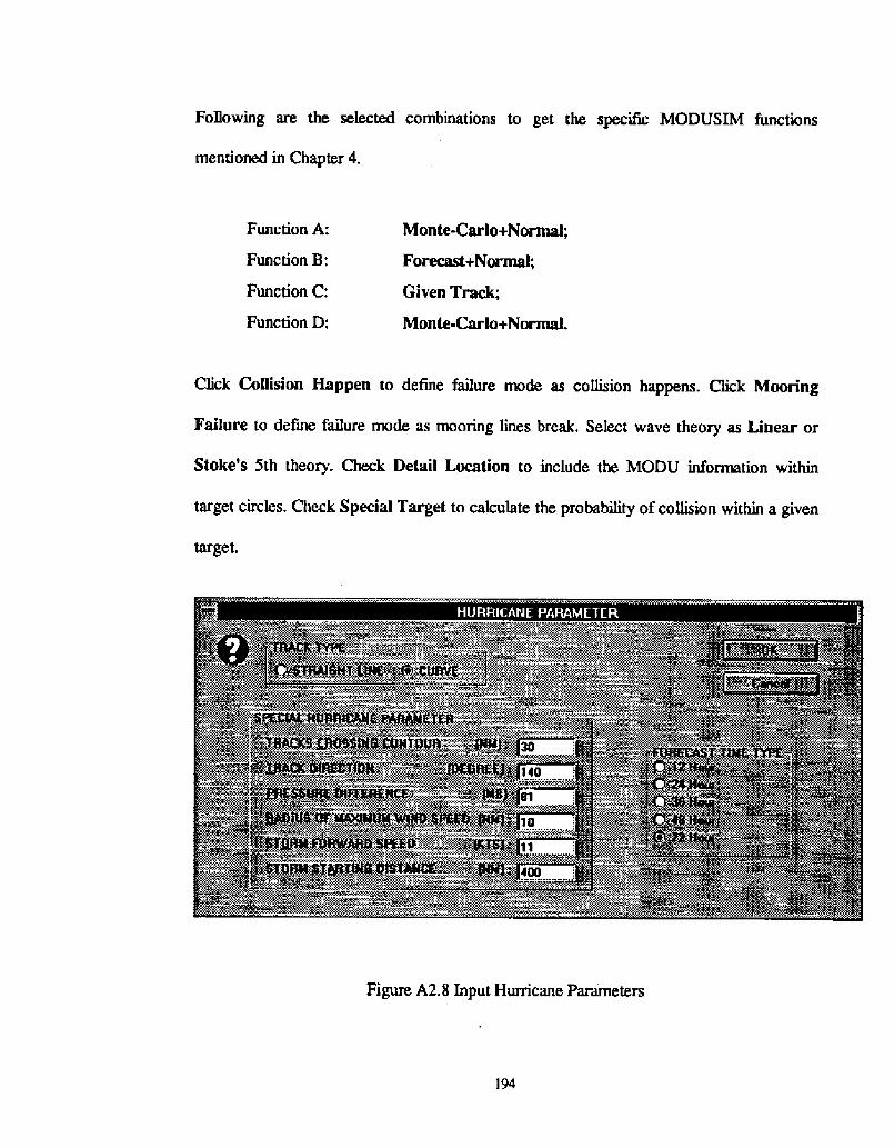
Following are the selected combinations to get the specific MODUSIM functions

mentioned in Chapter 4.

Click Collision Happen to define failure mode as collision happens. Chck Mooring

Failure to define failure mode as mooring lines break. Select wave theory as Linear or

Stoke's 5th theory. Check Detail Location to include the MODU information within

target circles. Check Special Target to calculate the probability of collision within a given

target.

Figure A2.8 Input Hurricane Parameters

Function A:

Function B:

Function C:

Function D:

Monte-Carlo+Normal;

Forecast+Normal;

Given Track;

Monte-Carlo+Normal.

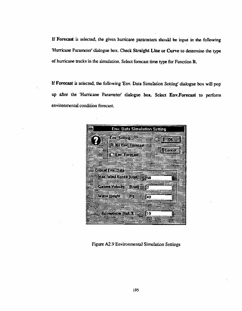
If Fo~ is selected, the given hurricane paranI:ters should be input in the following

'Hurricane Parameter' dialogue box. Check Straight Line or Curve to determine the type

of hurricane tracks in the simulation. Select forecast time type for Function B.

If Forecast is selected, the following 'Bnv. Data Simulation Setting' dialogue box will pop

up after the 'Hurricane Paraneter' dialogue box. Select Env.Forem4 to perform

environmental condition forecast.

Figure A2.9 Environmental Simulation Settings

195

If Given Track is selected, the 'Given Hurricane Track' dialogue box will pop up after the

'Simulation Type' dialogue box. Input the general hurricane information in the group of

Hurricane Parameter. There are at most eight points that can be input to describe the

hurricane track. DT is the time step between the adjacent points.

Figure A2.10 Given Hurricane Track Information

SIMUPARA command allows to input calculation coefficients. The dialogue box

'SIMULATION PPNAMETERS' will pop up when it is selected. Input the wind, wave

and current force coefficients in FORCE PARAMETERS, Select the type of current

velocity distribution in CURRENT TYPE, Select the time step between the re-calculation

of environmental forces in TIME STEP.

Figure A2.11 Input Calculation Coefficients

RAND PARA command aHows to input probability distributions of random parameters.

The dialogue box 'RANDOM PAFAMETER' will pop up when RAND PARA command

is selected.

197

Figure A2.12 Input Random Parameter Information

Note here, Lamta is the hurricane occurrence rate at a point in the selected reference per

year per nautical mile.

PARA CORRELATE command aUows to input correlation among random parameters.

The dialogue box 'PARAMETER CORRELATION' will pop up when it is selected.

198

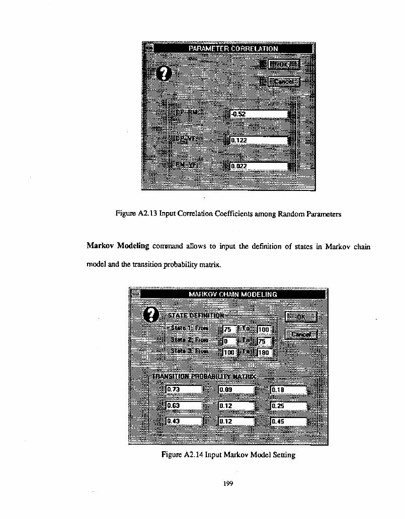
Figure A2.13 Input Correlation Coefficients among Random Parameters

Markov Modeling command allows to input the definition of states in Markov chain

model and the transition probability matrix.

Figure A2.14 Input Markov Model Setting

A2.4 Execute the Program

There ttuee commands under RUN menu;

RESET command allows to reset the program before each simulation.

RUN command is cbcked to begin the simulation. Before chck RUN, you should set up

@RISK simulation parameters. The recommended @RISK simulation settings is as in

Figure 2.12. After the simulation is completed, a dialogue box wiH pop up.

Figure 2.15 NRisk Simulation Setting

Strategy comn~d aHows to do strategy simulation to determine the best place to site the

MODU within the acceptable area.

A2.5 General Jackup Information

The MODUSIM has been updated to simulate the movement of bottom founded MODUs.

There are three command under the Jackup menu.

Jackup Type comtnar4 allows to determine the MODU type, foundation type and failure

Jackup Mo allows to input the general information of the jack-up.

Capacity allows to input the foundation capacity and leg capacity.

Figure A2.16 Jackup Type Input Information

201

Figure A2.17 GeneraI Jackup Input Information

Figure A2.1S Input Jackup Capacity Information

202

A3. Output

The output of MODUSIM can be in numerical and graphical format.

Click RESULT command for simulation result.

Figure A2.19 Simulation Result

Click RESUTAR for output of special target collision probability.

Figure A2.20 Simulation Result for Target Circles

Click Summary command for the simulation result from Strategy function.

Click Env.Restjlt to get the result from the simulation of the environmental conditions.

Figure A2.21 Environmental Condition Simulation Result

Click Histogram command to get the histograms of environmental condition. The

fo11owing 'Type of Histogram' dialogue box will pop up. Select different forecast time and

different forecast type of hurricanes.

205

Figure A2.22 Type of Histogram

Click Return command to return to the welcome screen.

In case of simulation the MODU's movement during a given hurricane, click ROUTE

command to get the MODU's moving route during hurricanes.

During the simulation of a given track, a dialogue box 'COLLISION HAPPENING' will

pop up whenever a collision happens. Click STOP HERE to stop the simulation. Click

NO REPORT to skip the 'COLLISION HAPPENING!' dialogue box after the following

co!lision. Click HOLDING and input HOLDING TIME to make the MODU stop at the

collision place for a while.

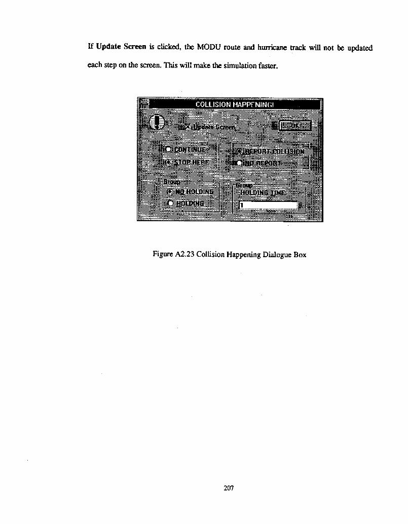
If Update Screen is clicked, the MODU route and hurricane track will not be updated

each step on the screen. 1%is will make the simulation faster.

Figure A2.23 Collision Happening Dialogue Box

207

APPENDIX B

EVACSIM

MODU Evacuation Procedure Simulation Program

User Manual

208

EVACSIM

MODU Evacuation Procedure Simulation Program

Copyright 1996

This software is provided "as is" by the Marine Technology and Management Group

MTMG! at University of California at Berkeley to sponsors of the research project

Securing Procedures for Mobile Drilling Units in the Gulf of Mexico Subject to

Hurricanes. Any express of implied warranties of merchantability and fitness for a

particular purpose are disclaimed. In no event shall the MTMG be liable for any direct,

indirect, incidental, special, exemplary, or consequential damages including, but not

limited to, procurement of substitute goods or services; loss of use, data, or profits; or

business interruption! however caused on any theory of liability, whether in contract, strict

liability, or tort including negligence or otherwise! arising in any way out of this software,

even if advised of possibility of such damage.

B1. Introduction

61.1 lntrocfuction

EVACSIM 1.0 is a computer simulation program developed for simulating the MODU's

evacuation procedures in humcanes. It is based on offshore evacuation simulation models

and associated weather-related downtine techniques developed for the extension research

of joint industry - government sponsored research project titled "Securing Procedures for

Mobile Drilling Units in the Gulf of Mexico Subject to Hurricanes".

This research has been performed at the University of California at Berkeley, Department

of Naval Architecture and Offshore Engineering by Research Assistant Jun Ying under

supervision of Professor Robert Bea, The theoretical background of EVACSIM is

documented in previous chapters of this report.

81.2 Application Range of EVACS1M 1.0

EVACSIM 1.0 can be applied to typical offshore platform evacuation procedure

simulations with project duration up to 3 days. With upgrade version, it can be used to

simulate more complex long-term weather sensitive offshore projects. The upgrade

version will be available upon request.

210

B1.3 Program Structure

The program is developed using Microsoft Project 4.0 and Excel 4.0 Software. The

following files are bounded together under the directory EVACSIM:

' ~ evacsuilmpp

~ merge. ftlp x

~ prtemp.mpx

~ ptemp 1.mpx~ temp.xlw~ input.xlw~ sinput.xlw~ sdata.txt

~ pdata.txt~ input.txt~ temp.txt

B1.4 Irtstaflation

B1.4.1 Backup Oisk

Before any instaHation begins, it is always a good practice to backup the program diskette

in the back of the report. We assume you are already familiar with DOS commands or

Windows operation. For example, in DOS you will need the DISKCOPY command to

make backup copies of your program disk.

B1.4.2 System Requlremertts

To run EVACSIM 1.0, you must have a 486 or higher based PC with 8MB RAM at least,

MS DOS 5.0 or higher, Windows 3.1 or higher, Microsoft Project 4.0, EXCEL 4.0 and

NRisk for Excel 3.1.

61.4.3 lristallation

To install EVACSIM 1.0, first copy all the files in the attached disk to your hard drive

under the directory "c evacsim". Then you can expend the zip Qle by type: pkunzip

evacsim.zip.

82. Input Data

82.1 Introduction

To run EVACSIM 1.0, you must start MS Project 4.0 and Excel 4.0 at the same time. The

program wiH transfer data between MS Project and Excel automatically. Then, in MS

Project, open the file evacsim.mpp under the directory c:Qvacsim.

The evacsimmpp has a evacuation procedure model which is performed on Zane Barnes.

The user may modify the model by adding or dropping some tasks or resources, changing

task duration or changing task relationship, etc., or even buiMing another new evacuation

procedure model All this operations may be done through tools in MS Project. Please

refer to MS Project user menu for detail operation procedures.

2i2

82.2 Input Hurricane Forecasting Data Information

The hurricane forecast data input file is pdata.tet. Me example input file is as follows:

Evacuation Simulation Input CardForecast Data Begin Time:11/03/95 00:00 AM

Forecast Data at �6.0,1143!:6,25,4.012/6,451828,4524393.030303536,30+542,35,6.048+2,8.054,62,9.7

60,43,7.166,323.67228,4.7

The file includes the forecast data beginning time: ll/03/95 00:00 AM; forecast data point

location.' �6.0,1143!; and every 6 hour forecast data for wind speed and wave height at

forecast location up to 72 hours after the forecast beginning time. The forecast data is

formatted as: hours to the forecast beginning time, wind speed and wave height. The units

can be chosen by the user, but should the same unit system with that used in the input file,

input.lxt.

213

82.3 Input Resource Environmental and Operational Down-TimeCriteria

To edit resource environmental and operational down-tirrM: criteria, click the command

Edit Resource under the Option Menu. The program wiII shift to MS Excel 4.0 and open

the file input.txt. The format of input.txr is as follows:

User can edit parameters directly in Excel worksheet. Restricted Resource Number is

the number of the resources which have environrrental or operational restrictions on them.

Here, five resources are listed. ID is the jd which is assigned to each resource in the MS

Project. They may be found in project view of resource sheet. Wind speed and wave

height are the two environmental criteria used here. The units should be the sarrm as that

in pdata,txt. Duration is the minimum continuous operational duration for each resource.

In All�!fHalf�! Day input, 0 means the resource can work day 8r. night and I means

214

only day time. ¹ of Sim is the latest evacuation start time of simulations in terms of hours

from forecast beginning time. And DT of Sim. is the interval in hours of different

evacuation start time. We last inputs, Number of Task to Be Checked, Task ID, ReaID

and Allover.Dur, are the number of un-separatable tasks, task id, associated resources id

and the maximum aHowable operating duration in hours.

After edit the resource parameters, click Return to Project command under the Project

menu to return to MS project.

B3. Simulation Procedure

The simulation procedure includes deterministic and probabilistic simulations.

83.1 Oeterrninistic Simulation

Click command Run Evac under the Option menu to perform the deterministic

simulation at a given evacuation start time. The program will pop a window for input of

the start time. The simulation result will give the whole project information, includes

duration of whole project and of each task, the critical path of the project, etc..

Click command Run Detsimu under the Option menu to perform the deterministic

simulation with the start time changed Rom 6 hours after the forecast beginning time to

the latest simulation evacuation start time which is inputted by the user, with DT hours

215

interval The program will shift to Excel to present the result. The result will be in chart

format as in Figure 5.6 and 5.7. Also, user can click command Forecast Data under

Project Menu to show a chart of forecast data as in Figure 5.5. Click Return to Project

to back to MS Project.

B3.2 Probabilistic Simulation

To perform simulation in probabilistic region, Grst step is to generate the random

environmental simulation data based on the forecast data. In the .Risk for Excel 4.0,

open the file sinputxlw, and follow the instructions to generate the data, then back to

project. Click command Run Probsimu under Option menu to begin the simulation in

probabilistic region. The simulation will take a1most 30 minutes for a typical 486-66 PC.

The program will present the simulation results in Excel chart format as in Figure 5.8. The

chart shows the probabilities of evacuation failure in different evacuation start time vs.

evacuation start tire. Chck command Forecast Data to see forecast information and click

Back to Project to return to MS Project.

216

APPENDiX CDISTRIBUTION FITTING

AND GOODNESS-OF-FIT TEST

C.1 Estimating

The goal of Distribution Fitting is to find the pararrM:ters of the distribution that best fits

the input data &om a group of parametric distribution families. The distribution families

used in this research are: Beta, Exponential, Lognormal, Normal, Rayleigh, Triangular,

Uniform and WeibulL These distributions are used because they are popular in engineering

applications. The fitting performed in the research finds a distribution from the distribution

families that best fits the input data.

Distribution fitting goes through the following steps to find the best fit for the input data:

~ For each distribution type, a first guess of parameters is made using maximum-

likelihood estimators;

~ The Chi-square is minimized using the Levenberg-Marqriardt method;

~ The fits of the best-fitting parametric distributions are compared;

~ The parameters of the overall best-fitting parametric model are reported as the

parameters of the best fit distribution.

ln principle, one should adjust the Chi-square using the number of fitted parameters in

model selection. That adjustment is not important here because the number of parameters

is about the same for aH models �-4!, and the number of data is large �0' -10'!.

217

C2 Maximum Likelihood Estimators

To fit a distribution to the data set, nonlitiear iterative procedures such as the Levenberg-

Marquardt algorithm need an initial set of parameters. The maxiinum likelihood estimators

are derived for each distribution function. The MLE of a set of paraneters are those

values that maximize the hkelihood function given a set of observation data For any

density function f x! with a parameter vectors, and a corresponding set of independent

observational data X�an expression called the likelihood may be defined.

C-l!

To find the MLE, one maximizes L with respect to tx by finding a stationary point

C.2!

and solving for a.

C.3 The Levenberg-Marquardt Method

The maximum likelihood estimator need not fiit the data best in a Chi-square. The

Levenberg-Marquardt Method is a nonlinear least-square solver which we can use to

improve the Chi-square fit beyond maximum likelihood, using MLE as an initial guess of

the parameters.

The Levenberg-Marquardt method does not find the absolute minimum for chi-square,

rather, it finds a local minimal. The performance of this method depends on the initial

218

parameters used. Therefore, a good first guess will produce a good result, while a poor

first guess might not provide a useful result.

The foHowing steps outline the Levenberg-Marquardt method:

1. Calculate the "first guess" of all parameters;

2. Find the goodness-of-fit of the input data to the function using these parameters;

3. Vary the parameters by an amount proportional to a factor m;

4. Measure the goodness-of-fit with the modified parameters;

5. If the modified parameters produce a better fit, update the parameters with these

values and decrease the value of m by an order of magnitude;

6. If the modified values produce a worse fit, do not update the pararrM:ters; increase the

value of m by an order of magnitude;

7. Return to step 3.

These steps are repeated until it finds that varying the parameters has little effect on the

goodness-of-fit measured as the percentage change in the chi-square value!. This point is

a local minimum of the goodness-of-fit statistic, the sum of squared residuals.

C.4 Goodness-of-Fit Test

The process of calculating MLEs and minirni'~g the sum of squared residuals gives a

"best guess" for each distribution. Then we measure whether each fiit is probabilistically

adequate using goodness-of-fit statistics.

2!9

We can characterize the goodness of fit by the probability that the data would be obtained

if the fitted model were correct. This probability is called the P-value. If the P-value is

small, the data cast doubt on the validity of the model. If the P-value is large, the data are

compatible with the model.

There are a lot of goodness-of-fit tests, e.g., chi-square, Kolmogorov-Smirnov and

Aderson-Darling. The Chi-Square is the most common.

Chi-Square Test:

The Chi-Square test is the most common goodness-of-fit test. It can be used with any type

of data and any type of distribution function. A weakness of the Chi-Square test is that

there are no clear guidelines for selecting intervals number of classes!. In some situations,

one can reach diferent conclusions &om the same data depending on how the intervals are

chosen.

The Chi-Square statistic is defined as:

C.3!

where

P. = the observed probability of the data in the ith histogram bin

p, = the theoretica1 probability that a value will fall with the X range of the

ith histogram bin

220

Kolmogorov-Sirnirnov Test:

The Kolmogorov-Simirnov Test does not depend on the number of intervals. A weakness

of the Kolmogorov-Simirnov Test is that it does not detect tail discrepancies very well.

The Kolmogorov-Smirnov statistic is defined as:

D =sup F x! � F x! C.4!

where

n = total number of data points

F x! = the hypothesized distribution

F x! = N n

N = the number of X.'s less than x.

The Anderson-Darling Statistic is:

A' = n f [F x! � F x!j 'P x! f x!dx C.5!

where

+2

F x![I � F x!]

221

Anderson Darling Test:

The Anderson Darling Test is very similar to the Kolmogorov-Simirnov Test, but it phces

more emphasis on tail values. It does not rely on the number of classes.

f x! = the hypothesized density function

F x! = the hypothesized distribution function

F x!=N

n

N = the number of X,' s less than x.

C.5 Confidence Levels and Critical Va/ues

The goodness-of-fit statistic teHs how probable it is that a given distribution function

produced the data set. But how good is good enough? A critical value is the value in a test

that separates the rejection region from the acceptance region. For the goodness of fit

tests, this value determines whether or not one should reject a fitted distribution.

Statistical hypothesis testing provides a structured analytical method to make a decision

regarding fit test results. This method aHows one to control or measure the uncertainty

involved in the decision.

In the case of research work here, the decision we need to make is whether the input data

were generated Irom the distribution function reported as the estimate. The critical value

involved is a goodness-of-fit measurement that is compared to the goodness-of-fit of the

best fitting distribution.

The significance level, a, is the probabiTity of rejecting the null hypothesis in this case,

that the estimated distribution is correct! when it is true. In other words, a smaH value of

222

ct decreases the probability of incorrectly rejecting the null hypothesis that a given set of

parameters produce the input data.

For the chi-square test, the critical value is the 1- a percentile of a chi-square distribution

with N-1 degrees of freedom N is the number of classes!.

1.0

0.f

0.0 0.0 6.9 11.1 17.8 23.7 29.6Critical V*ltra

A Chi-Square Distribution with 10 degrees of freedom

When the calculated Chi-Square statistic is larger than the critical value, the null

hypothesis should be rejected the distribution is not a good fit!. Equivalently, one should

reject the null hypothesis when the P-vahe is less than the significance leveL

Critical values for the Anderson-Darling and Kolmogorov-Smirnov goodness-of-fit

statistics have been found by Monte-Carlo studies, detail can be found in References.a

v'I ',