Institute for International Economic Policy Working Paper Series Elliott School of International Affairs The George Washington University

Taxes, Prisons, and CFOs: The Effects of Increased Punishment on Corporate Tax Compliance in Ecuador

IIEP-WP-2011-2

Gabriela Aparicio The George Washington University

Paul Carrillo The George Washington University

M. Shahe Emran IPD, Columbia University

April 2010

Institute for International Economic Policy 1957 E St. NW, Suite 502 Voice: (202) 994-5320 Fax: (202) 994-5477 Email: iiep@gwu.edu Web: www.gwu.edu/~iiep

1

Taxes, Prisons, and CFOs: The Effects of Increased Punishment on Corporate

Tax Compliance in Ecuador1

Gabriela Aparicio

The George Washington University

Paul Carrillo

The George Washington University

M. Shahe Emran

The George Washington University

And IPD, Columbia University

Abstract: This paper takes advantage of a rich firm level data set from Ecuador to analyze the effects of a

reform in 2007 that introduced imprisonment for tax evasion and made a firm’s CFO liable for tax-crimes.

Our dataset contains actual tax-return and financial-statement information for the universe of corporations in

Ecuador from 2003 to 2007. We study the effects of higher punishment both at the intensive and extensive

margins. We combine a difference-in-difference-in-difference approach with the DiNardo, Fortin and

Lemieux decomposition method. This allows us to estimate the heterogeneous effects of the reform across the

distribution of firms. We find that, at the intensive margin the reform led to an average 10% increase in real

corporate tax payments. However, positive effects are only found at the right tail of the tax distribution (above

the 75th percentile). At the extensive margin, the probability of entry into the tax-net increased, but most of the

firms that entered the tax net claimed zero taxes.

Keywords: Tax evasion, corporate tax compliance, tax reform, developing country, punishment,

Ecuador

JEL Codes: H26, H32, O12

1 We thank Dilip Mookherjee, and conference participants at the 2011 AEA Meetings at Denver and the 2010 LACEA

Annual Conference for helpful comments and discussions. We are especially grateful to the Ecuadorian Tax Authority

(Servicio de Rentas Internas SRI) staff for their collaboration and for providing access to the data used in this study. In

particular, we are indebted to its Director, Carlos Marx Carrasco, and to Miguel Acosta, Byron Vázconez, José Ramírez,

Edwin Buenano, and Carlos Uribe among many others. All confidential data has been handled according to the

Ecuadorian data confidentiality laws.

2

1. Introduction

Tax administration and compliance have long been the weakest links in tax reform in

developing countries. In the last few decades, significant tax reform has been implemented in a large

number of developing countries under the structural adjustment and stabilization programs of the

World Bank and IMF. The focus of the reform has, however, been on the tax structure, i.e., tax bases

and rates, most notably on introducing value-added tax (VAT) and reducing trade taxes (especially

import tariff).2 Although most of the tax reform programs include some administrative components,

they are usually accorded only a supportive role at best. The widely implemented tax reform

program that instituted VAT as a main source of government revenue has, however, failed to

compensate for the revenue loss due to drastic reduction in tariff rates, especially in poor developing

countries (see, Baunsguaard and Keen (2010), Rajaraman (2004)).3 This difficult fiscal predicament

makes it especially important to understand the revenue effects of tax administration reform in

developing countries; given a certain tax structure, how much difference a better monitoring (higher

audit probability) or an increase in the punishment can make to government revenue?

In spite of the importance of the topic, the empirical literature on tax enforcement and

compliance is limited at best, especially in the context of developing countries where the required

data are rarely available (among the few studies available, see Das-Gupta and Mookherjee (1998),

Mclaren (2003)).4 Even in the context of developed countries, attempts to establish an empirical link

between better administration and the extent of evasion have been less than satisfactory because of

difficulties in getting data from actual tax-returns, and identification challenges due to unobserved

heterogeneity. This paper provides evidence on the effects of higher punishment (both monetary and

non-monetary) on corporate tax revenue by analyzing a rich firm level data set from Ecuador, where

imprisonment for 1 to 6 years was introduced in 2007 as a punishment for tax evasion as the center

piece of a new tax enforcement regime.

There is a rich body of theoretical work on tax evasion in the economics literature (see,

Allingham and Sandmo (1972), Srinivasan (1973), Cowell (1990), Das-Gupta and Mookherjee

(1998), Mookherjee and Png (1994), Slemrod and Yitzhaki (2002), among others). The basic model

as developed by Allingham and Sandmo (1972) adopts the `crime and punishment' framework that

2 For recent discussions on the tax policy reform in developing and transition countries, see, for example, Gordon, R, ed.

(2010), Gordon (2010), Whalley and Kononova (2010), Boadway and Sato (2009), Emran and Stiglitz (2005, 2007). 3 Most of the governments in developing countries have turned to domestic borrowing to cover the revenue shortfall.

This has caused a dramatic increase in domestic debt in developing countries with the attendant consequences such as

crowding out of private sector credit (see Emran and Farazi, 2009). 4 In the context of developing countries, the empirical literature on corporate tax compliance is particularly scarce, even

though corporate taxes have traditionally accounted for as much as one third of tax revenues (a much higher share than in

developed countries) (Burgess and Stern (1993), and Avi-Yonah and Margalioth (2006)).

3

grew out of the influential work of Becker (1964). In the standard model with risk neutral

preferences, the decision to evade taxes depends on the expected cost (probability of getting caught

times the punishment) and benefit (savings from tax evasion).5 A widely discussed implication of the

Becker type models is that the optimal fine is maximal, because while both monitoring and fines

increase compliance, the first is more costly than the latter.6 There is, however, a large literature that

investigates why, in general, we do not observe maximal fines in the real world (for a survey of the

literature, see Polinsky and Shavell (2000)). One important factor which is especially relevant for the

developing countries is credit constraints, or more generally wealth constraints. The threat of a large

fine has little bite if the tax payer does not have the money to pay the fine.7 Another important issue

in the context of developing countries is the weak legal capacity that may make it very costly for a

tax authority to enforce the fines.

Since the scope for monetary punishment is relatively limited in developing countries, non-

monetary punishment schemes including imprisonment for tax evasion assume added importance. If

the threat of imprisonment is credible enough, it might affect the behavior of tax payer without

requiring significant expansion in prison space. A credible threat of imprisonment, not the actual

imprisonment, is important for tax payers’ behavior.8 Thus from a policy perspective, the threat of

imprisonment seems to be an attractive instrument to improve taxpayer compliance in developing

countries. However, note that the effects of higher punishment depend on the extent of corruption in

tax administration. If most of the tax inspectors are corrupt, a higher punishment can make things

worse for both the taxpayer and government (Stiglitz (2010), Emran and Stiglitz (2007)). Since the

threat of imprisonment increases the bargaining power of tax inspector vis. a vis. the tax payer, the

bribe amount will in general go up. But this may not increase government revenue as the inspector

gets rich at the expense of both taxpayer and government. The effect of a higher punishment for tax

evasion on government revenue is thus an empirical question. However, to the best of our

knowledge, there is no empirical work in the current economics literature that attempts to isolate the

effects of introducing higher punishment on the behavior of taxpayers and tax revenue in a

developing country.9

5 Crocker and Slemrod (2005) extend the standard model to study corporate tax compliance. They find that a sanction on

the CFO has greater deterrent power than a sanction on the corporation itself, since the latter can be passed-on only

imperfectly to the party making decisions. 6 In theory, one can keep the expected cost for the taxpayer unchanged by increasing the fine arbitrarily while reducing

the monitoring (auditing) close to zero. 7 An important part of the problem is lack of information on the ability to pay. For example, most of the firms in

developing countries operate in the informal economy with little verifiable accounting data. This makes it especially

difficult to use monetary punishment as a credible threat. 8 In a repeated game model, one should not observe any imprisonment along the equilibrium path.

9 Interestingly, most of the policy discussion on tax administration reform focuses on the incentives of the tax inspectors,

and the possible collusion between the tax payer and tax inspector (corruption). The literature, especially the empirical

work, has largely ignored the role of higher punishment given a monitoring regime.

4

This paper takes advantage of a rich firm level data set to analyze the effects of a reform to

the tax code in Ecuador during 2007 that introduced higher punishment for tax evasion. Although the

2007 reform imposed both monetary and non-monetary punishment, at its core was a highly costly

and visible non-monetary punishment: the new legislation introduced reclusion from 1 to 6 years as

a punishment for non-compliance, and made a firm's general manager (CFO) and anyone else

involved in the tax evasion scheme liable for a criminal offense. Note that imprisonment is a

fundamentally different form of punishment that entails potential social cost (loss of reputation in the

society) for the family as a whole in addition to the cost to the evader himself/herself. Because of

this special nature of imprisonment as a punishment for tax evasion, it stood out as the salient feature

of the 2007 tax reform.10

Furthermore, given that increased monetary punishment for tax evasion

was in the form of higher interest rates on arrears and surcharges (20 percent), we are able to isolate

the effect of non-monetary punishment (from that of monetary punishment) by including tax arrears

as a control in our regressions.11

The 2007 reform offers us an excellent opportunity to understand the impact of higher

punishment as a tax enforcement instrument in a developing country for a number of reasons. First

of all, the tax authority in Ecuador has a very good reputation, providing an environment in which

the threat of higher punishment is likely to be credible.12

Second, by leaving most of the tax

parameters unchanged,13

the 2007 reform allows us to isolate the effects of one particular component

of the reform (i.e. punishment) given a tax rate structure. Indeed, a major difficulty in estimating the

effects of higher punishment on tax evasion is that tax reforms are usually omnibus reform that

implements an array of changes simultaneously such as changes in types of taxes (for example,

introduction of VAT), rates (changes in tariff and VAT rates are common), and enforcement

mechanisms (for example, hiring of new tax inspectors, higher wages for tax inspectors and higher

punishment for corruption by tax officials). The corporate tax rates were not affected by the 2007

reform, and there is no evidence that monitoring and enforcement improved in any significant way.

We study the effects of higher punishment on corporate tax compliance both at the intensive

and extensive margins. For the intensive margin, we use the subset of firms that belongs to the tax-

net for consecutive years, and for the extensive margin, we focus on the entry into and exit from the

tax net using the universe of firms across different years. Moreover, by combining the difference-in-

difference (DD) approach with the DiNardo, Fortin and Lemieux (DFL) decomposition method, we

10

Most of the discussion in the media and among general people focused on this aspect of the reform. 11

This is done under robustness checks in section 5.5. 12

The tax administration in Ecuador started operations as an independent agency in 1997. According to Mann (2004),

this new entity achieved significant improvements in tax collection because “since inception the SRI has had only one

Director who is well known for her honesty and competence”. Similarly, according to World Bank (2003), “the creation

of the Internal Revenue Service (SRI in its Spanish acronym) as an independent entity and its strengthening in the late

nineties brought about a significant recovery in non-oil tax revenue.” 13

Most tax parameters remained unchanged, not only in 2007, but throughout the entire duration of our dataset (2003-07)

5

are able to estimate the heterogeneous effects of the reform across the distribution of firms, without

imposing any arbitrary functional form.14

Although most of the empirical literature on tax reform

deals with the mean (i.e., the average) effects, the mean effects might mask important heterogeneity

across different firms. Moreover, the possibility of heterogeneous effects has implications for both

revenue and equity effects of a tax reform.

There are many plausible theoretical reasons to expect the effects of a higher punishment on

firms to be heterogeneous. For example, small firms may respond differently because audit resources

are usually not concentrated on the lower tail of the firm distribution. Also, new startup firms, that

are usually smaller in size, are likely to be significantly less risk averse and thus may discount the

cost of higher punishment. In contrast, firms in the middle and top of the distribution may react more

strongly to changes in punishment because they are visible to tax inspectors and they are subject to

more intense monitoring. Moreover, it may only be cost-effective for the tax authority to punish

large firms, for which the revenues that are recovered exceed the costs of taking the firm to court.

To estimate the effect of the higher punishment, we use difference-in-difference (DD) and

difference-in-difference-in-difference (DDD) approaches, exploiting the fact that we have data on a

number of years before the reform was implemented (2003-2006). The main identification challenge

in our application is that the effects of the 2007 reform on revenue may be confounded by other

secular factors such as sustained economic growth and small but steady improvements in tax

administration.15

The increase in tax revenue between 2006 and 2007 thus cannot be attributed solely

to the increased punishment for tax evasion even though there was no change in the corporate tax

rates and no significant improvements in the enforcement regime, especially as it relates to firms.

We thus need to construct the counterfactual trend in revenue growth that would have been observed

in the absence of the 2007 reform. The availability of data for four years before the reform allows us

to understand the underlying trend with a measure of confidence, and also to construct the

counterfactual trend in a variety of ways. For example, we calculate alternative trend lines across the

distribution of firms using data from different pairs of consecutive years, and then take the upper

envelope of the different trends as a conservative estimate of the counterfactual trend in corporate

tax revenue in the absence of the reform. An alternative is to use the average of the different trends

14

To the best of our knowledge, ours is the first paper in the literature to combine difference-in-difference with the DFL

method to estimate heterogeneous effects of tax policy on firms. 15

Note that in most of the available studies in economics that use difference-in-difference method, data consists of only

one period before the treatment (usually baseline surveys in evaluation studies), which makes it difficult to estimate the

underlying trend in the absence of intervention, and one cannot test the validity of the “parallel trend” assumption. The

fact that we have data for four periods before the “intervention” (i.e., 2007 reform) makes it easier for us to estimate the

counterfactual trend. One might argue that compared to a standard difference in difference set-up our data set suffers

from the fact that we do not have a `control group’ in the same period of time. However, observe that most of the

objections to the validity of difference-in-difference strategy emanates from the fact that the control group may not be a

good representation of the treatment group in the counterfactual state. In our case, the control group is exactly the same

firms, but observed in a different time period.

6

as an estimate of the counterfactual trend. The average may represent the counterfactual trend more

faithfully if the year-to-year changes in corporate income tax revenue are affected significantly by

transitory shocks. To address the possibility that the underlying trend is not linear, and may be a

convex function of time (i.e., the year-to-year revenue changes are increasing over time in the

absence of the reform), we implement a triple difference (DDD) approach.

In the context of our application, where we rely on variations over time for estimating the

revenue effect of the reform, the estimates might be misleading if the year of the reform was

exceptional in terms of economic performance. For example, if the economy experienced a strong

positive productivity shock; then, the corporate tax revenue might be driven by firms’ higher growth

and sales revenue rather than by the threat of imprisonment. However, 2007 was not above the trend

in terms of economic performance, the growth rate in GDP was 3.6% and in manufacturing value

added was 3.8% in 2007 compared to 4.8% (GDP) and 4.7% (manufacturing value added) for the

period 2003-2006.16

Thus an increase in tax revenue between 2006 and 2007 is not likely to be

driven by common positive shocks to growth such as productivity or price shocks.17

As an additional

layer of caution, we control for the sales revenue of firms in the regressions.18

At the intensive margin, results suggest that there was a large and positive `mean effect’

(about 10 percent) of increased punishment on tax revenue. In other words, for firms that were

already in the tax net before the reform, tax payments went up by about 10 percent on average.

However, the effects were heterogeneous across the tax distribution. For example, tax revenues did

not increase at the 40th

quantile, but they increased by 14 percent at the 90th

quantile (based on the

DD specification). Thus, focusing exclusively on the mean estimates can mask important

heterogeneity in the impact of tax reforms. At the extensive margin, results suggest that the

probability of entry into the tax-net increased due to higher punishment in 2007 as compared to prior

years (2003-06). However, most of the firms that entered the tax net in 2007 actually claimed zero

taxes, and consequently they did not contribute to increasing the government’s tax revenue.

The rest of the paper is organized as follows. Section 2 provides institutional details about

Ecuador’s Tax Administration and the 2007 reform. Section 3 describes the data. In section 4, we

present the empirical strategy to measure the mean impact of the 2007 reform at the intensive

margin. Section 5 measures the impact at several points of the tax distribution. In Section 6, we

discuss effects of the reform at the extensive margin. Finally, section 7 concludes.

16

However, non-oil GDP growth performance was better. 17

One important price shock especially for government revenue in Ecuador is oil price. To make sure that our results are

not driven by the oil revenue, we exclude the firms in the oil sector. 18

We would expect a firm to report higher sales when declaring higher tax liabilities as a response to higher punishment.

This implies that by controlling for the sales revenue, we might be underestimating the effects of punishment. It is

interesting that we still find substantial effects of higher punishment on corporate income tax revenue.

7

2. Taxation in Ecuador

In this section, we provide some institutional details about Ecuador, its Tax Administration

(SRI) and, most importantly, the 2007 Tax Reform.

2.1. General background

Ecuador is a developing country in South America. In 2006, its per capita GDP was close to

US$ 3,200 –lower than most of the other countries in this continent except Bolivia and Paraguay.

Ecuador’s economy relies heavily on the oil industry. Oil exports accounted for about 55 percent of

its total exports and approximately 25 percent of the Central Government revenue came from oil-

related royalties in 2006. Agriculture is the second most important sector.

In Ecuador, all firms are taxed 25% of their profits.19

Reinvested profits are taxed at a rate of

15% (Deloitte 2010). Moreover, all corporations are required to distribute 15% of pre-tax profits

among their employees. Although these tax obligations may seem high, the typical corporate tax

burden in Ecuador is lower than in other countries in the region. The tax base is defined as the sum

of ordinary and extraordinary revenues subject to tax, less production costs and other discounts and

deductions.20

Profits are taxed equally regardless of whether they are retained or distributed. Special

provision laws may allow for additional tax breaks.21

The fiscal year in Ecuador coincides with the calendar year (ending December 31). All

corporations must file an annual profit tax return at the end of the tax year –between February 1st and

May 10th

– according to a deadline that varies with the corporation’s tax registration number. Each

corporation assesses its own profit tax, but tax authority usually revises those assessments on

subsequent inspections within specified time limits (Deloitte 2010). Virtually all revenue received by

corporations is subject to income tax withholding (Deloitte 2010).22

The tax withheld is usually an

advance payment of the recipient’s profit-tax and may be used to offset the total annual tax due. The

SRI has the power to adjust withholding rates without approval of the legislature.

The SRI classifies corporations into different groups, which may face higher levels of

monitoring. The most relevant is the Large Taxpayer Unit (LTU). LTU taxpayers –locally known as

19

Corporate taxes in Ecuador fit the economic definition of a “profit” tax, rather than an “income” tax, because

production costs are deductible. 20

Companies in certain sectors such as petroleum, construction, urban development, and real estate dealings, may

compute taxable income in accordance with special rules (Deloitte 2010). 21

For instance, there is a Hydrocarbons Law specific for the oil sector; Tourism and Mining Laws provide their own set

of tax breaks; and Regional-development Laws offer tax incentives for investments in certain provinces (EIU, 2006). 22

The withholding system is a mechanism where most companies (those that are designated by the SRI to be withholding

agents) are required to deduct and withhold a fixed percentage of the payments they make to other firms. We refer to this

fixed percentage as the withholding rate. This deduction takes place only if the payment is taxable income for those who

receive it. Every month, withholding agents must report and transfer all withholdings to the tax authority. Firms can

deduct their withheld funds from their tax liability.

8

“special taxpayers”– are the firms of greatest economic importance (usually measured by their sales

and employment levels) within each sub-region in the country.

2.2. The 2007 Tax Reform

During the last decade, taxation in Ecuador has faced a number of profound changes.

Taxation in Ecuador may be classified into three periods: (a) a period of policy instability

accompanied by deep administrative reform between 1997 and 2003; (b) a period of relative status-

quo –lack of structural tax reform accompanied by a consolidation of earlier administrative

improvements– between 2003 and 2006; and (c) a major tax reform in 2007. To avoid cluttering the

text, in this section we focus on the 2007 reform (details about earlier reforms can be requested from

the authors).

In 2007, reducing tax evasion and improving tax collection became a primary objective of a

new presidential administration. At the end of December 2007, the Ecuadorian constitutional

assembly passed a major tax reform bill, known as “Reform for Tax Equity”. Although the 2007 Tax

Reform introduced a variety of changes affecting several types of taxpayers (i.e. individuals and

corporations), it left most of the tax parameters unchanged in so far as firms are concerned. A

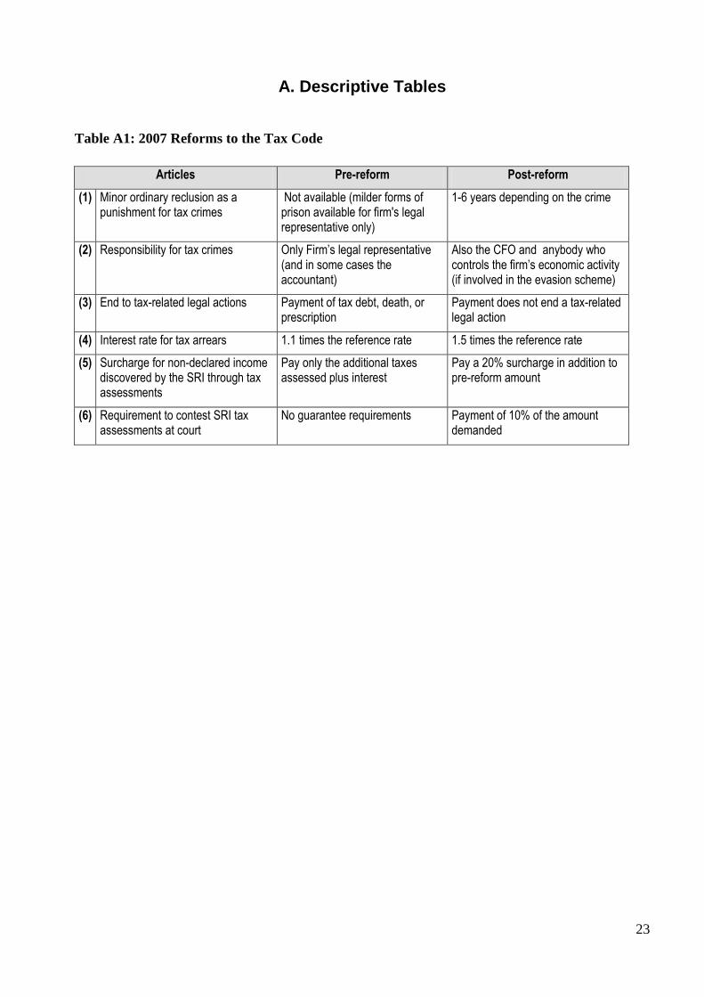
summary of the tax changes introduced in 2007 which are relevant for corporations is presented in

Table A1.

The most notable aspect of the 2007 tax reform is the introduction of more rigorous

sanctions.23

Most importantly, minor ordinary reclusion from 1 to 6 years was introduced as a

punishment for tax evasion. Moreover, legal actions can no longer be extinguished through the

payment of tax liabilities as occurred prior to 2007. In addition, while in the past only a company’s

legal representative or accountant were responsible for tax-crimes, now this responsibility extends to

anyone in the company who may have been part of a tax evasion scheme, and in particular the CFO.

Also, the new legislation increased fines and surcharges charged to firms that fail to pay their tax

obligations.24

Another change in the tax regime that can potentially confound our estimates of the

effects of higher punishment is the increases in the withholding rates in 2007 implemented through a

SRI decree. Fortunately, we have data on both tax arrears and taxes withheld by third parties; and

we include them as additional covariates as part of the robustness checks.

23

Besides tougher sanctions, the 2007 tax reform introduced a few other changes, most of which, however, affect only

multinational corporations which are not part of our sample. For example, multinationals are impeded from transferring

profit to related parties located in tax-heavens. 24

The interest rate for tax arrears increased from 1.1 to 1.5 times the reference rate (the 90-day active referential interest

rate of the Central Bank), and a surcharge of 20% of the principal must now be paid for non-declared income that is

discovered by the SRI through tax assessments. Prior to the reform, taxpayers were charged only the additional tax

assessed plus interest.

9

The timing of the reform is also fortuitous for our empirical analysis. The new measures

came into effect in January 2008; however, given that tax-returns for a given year are filed in April

of the following year, some parts of the new legislation –in particular more severe sanctions for tax

evasion– effectively apply to the 2007 tax-year. Interestingly, given that the reform was passed at the

end of the tax year, firms could respond to higher punishment by adjusting how they fill-out their tax

returns, but they were unable to change their actual behavior.25

On the administrative front, although the leadership of the SRI changed in 2007, the SRI

continued with prior efforts to modernize tax administration. There is, however, no evidence that the

enforcement and monitoring regime changed in any significant way in 2007. This is important for

our analysis because if enforcement and monitoring become significantly more efficient in 2007,

then it will be difficult to isolate the effects of higher punishment. Nevertheless, there is no evidence

that the audit risk increased in 2007 for most of the firms. Indeed, it is highly unlikely that audit risk

increased for most of the taxpayers given the tight resource constraints of the SRI. Moreover,

according to the available SRI data, the number of audits (of certain types) decreased in the Northern

Tax Office, where most firms are located. Although the enforcement and monitoring regime did not

change in any significant way in 2007, the average monitoring intensity still can change with

changes in the number of firms selected into the LTU where firms are subject to enhanced

monitoring. The number of firms that are selected into LTU varies substantially from year to year

without any clear trend. For example, the number of new LTU firms was 818 in 2007, 228 in 2006,

574 in 2005, 97 in 2002, and 840 in 1999. To allay any concerns that at least part of the revenue

response observed in 2007 may be due to the increase in the number of LTU firms, we report results

using a sample that excludes all of the LTU firms. It is reassuring that we find that the main results

of the paper are robust to such changes in the sample of firms.

Finally, in 2007, the SRI also exercised its power to decree a hike in the withholding rates.

In July 2007 there was a hike in withholding rates for most economic sectors (from 1 to 2 percent),

excluding the transport sector. To check if the estimated revenue increases in 2007 can be due to

changes in withholding rates, we report results as part of robustness checks that control for the total

withholding amount in the rgressions (please see section 5.5).

3. Data Description

The data used in this paper were obtained from SRI administrative records. The database

25

This may result in underestimating the overall impact of the 2007 reform, because some improvements in compliance

require changes in actual behavior. Such underestimation could be mitigated if firms expected an increase in punishment

at the beginning of the tax year. However, while the possibility of introducing reclusion as a punishment for tax evasion

was mentioned by the tax authority early in 2007; the text of the reform was subject to numerous and significant changes

throughout the year, and it was not clear whether the reform would actually be approved until December 2007.

10

contains information on every line-item of the universe of profit tax returns filed by public and

private corporations in Ecuador. Regardless of profitability, all corporations are required to file

profit taxes using Tax-Form 101, which contains information on the firm’s balance sheet and income

statement.26

The requirement that all corporations file a tax return is not inconsequential for our

analysis, as it leads to censoring in corporate profit taxes (roughly 30% of firms claim zero taxes in

any given year).

For the empirical analysis at the intensive margin, we focus on the sample of firms that file a

tax return in consecutive periods, and for the extensive margin, the focus is on the probability of

entering/exiting the tax net. In both cases, we exclude from the sample the firms that belong to the

public sector or that operate in the oil industry because they are subject to special taxation rules. All

nominal variables are deflated, to allow for meaningful comparisons across years, using the CPI

from the Ecuadorian Central Bank.27

However, some further adjustments were made to the data

sample used to study the intensive margin.28

Specifically, the sample for the intensive margin

focuses exclusively on firms that were created in 2003 or earlier, in order to control for the impact of

firm creation and to control for tax policies that encourage firm closure and reorganization as new

ventures.29

The resulting number of observations is approximately 24,000 firms per year (at the

intensive margin).

Table A2 presents summary statistics by year for the main variable of interest –corporate tax

revenue– both in levels and logarithms. We notice that there is an underlying positive trend from

year t to year (t+1) over the span of the pre-reform period (2003-2006), suggesting that it is not

unusual to observe an increase in average corporate tax revenue in Ecuador. However, we also

notice that while mean reported profit taxes between 2003 and 2006 increased at a similar annual

rate; profit taxes increased notably more during 2007.30

Indeed, it is not surprising that reported

taxes between 2003 and 2006 do not deviate much from the trend as no major tax reforms were

introduced during this period.

26

This form can be requested from the authors. 27

Applying the same deflator to all regions in Ecuador is appropriate as most corporations are concentrated in the two

major provinces –Guayas and Pichincha. Results are similar when using other price measures such as the wholesale price

index. 28

This sample includes only firms that file a tax return in consecutive years. We also excluded from this sample

observations with inconsistencies (i.e. negative revenues, etc.) and outliers. 29

The pattern of the results is similar when including in the data sample firms created after 2003, and/or firms that fail to

file a tax return in consecutive-years. 30

To understand the trend in corporate taxes, we estimated the following model:

titti uItrendY ,(0.37)(0.16)(0.61)

, )2007(1.581.29 6.29 (robust SE in parenthesis).

The model suggests, that while that tax revenue generally increase by $1,200 year-on-year, in 2007 tax revenue increased

by $1,500 above the trend. The model also suggests that an unusually large increase in corporate tax revenue between

2006 and 2007 cannot be explained by unusually low taxes in 2006.

11

Table A3 presents summary statistics for firms’ observable characteristics. The choice of

these variables is motivated by a close reading of the Ecuadorian tax law, and also the literature on

corporate tax compliance and effective tax rates (ETRs).31

The variables include revenue and total

assets as measures of the size of the firm and its performance. According to prior empirical evidence,

the effect of these variables on tax compliance of a firm is, however, not unambiguous (Rice, 1992;

Hanlon and Slemrod, 2005; Spooner, 1986; Kim and Limpaphayom, 1998). Other covariates include

fixed to total assets, leverage, and purchases (costs). These variables should reduce tax payments due

to the deductibility of capital investments, interest payments, and costs (Gupta and Newberry, 1997;

Porcano, 1986; Stickney and McGee, 1982). In the robustness checks sub-section (section 5.5), we

include additional covariates that are specific to our application. We control for withholdings to

isolate the impact of hikes in withholding rates (from 1 to 2 percent of income) occurring in mid-

2007; and we include tax arrears in order to try to isolate the prison effect (non-monetary

punishment) from increases in the interest rate on tax arrears (monetary punishment).

The inclusion of sales and costs as covariates deserve some additional explanation.

Controlling for these variables helps to account for possible demand shifts due to macroeconomic

conditions (such as GDP and exports growth), and it also helps to account for factors affecting firms’

costs such as productivity shocks and changes in imported intermediate input costs. Without any

controls for the exogenous changes in the demand or cost conditions, the estimated response in profit

taxes in 2007 is likely to capture the resulting changes in the true profitability of the firms, rather

than the exclusive effect of the higher punishment. However, note that we would expect a firm to

report higher sales and/or lower costs when it declares higher tax liability as a response to higher

punishment. Thus, by controlling for sales and costs, we are potentially underestimating the impact

of punishment on compliance. Interestingly, however, we find that the 2007 reform has a positive

revenue impact even when sales and costs are held constant. This may reflect the fact that firms in

Ecuador may misreport not only profits, but also other line items in their tax returns such as

exemptions.32

If we estimate the revenue response without controlling for a firm’s sales and costs,

the estimated effects of 2007 reform are larger. These estimates can be viewed as upper bounds on

the positive tax response to higher punishment. We do not report these results for the sake of brevity,

and they are available from the authors.

31

As pointed out by Hanlon and Slemrod (2005), to the extent that low effective tax rates (ETRs), defined as total tax

expense divided by pre-tax earnings, are a proxy for aggressive tax positions, variables that explain differences in ETRs

may help explain other measures of tax non-compliance as well. 32

Klepper and Nagin (1989) find that taxpayer misreport different line-items, according to opportunities for evasion.

Moreover, large firms usually have sophisticated accounting departments that allow them to engage in complex tax

avoidance schemes.

12

4. Effects of 2007 Reform: Intensive Margin

4.1. Empirical Strategy

In the introduction, we discussed a host of issues that arise in estimating the effects of higher

punishment for tax evasion with panel data. We also underscored some important advantages of the

2007 reform in Ecuador and the panel data set used in this paper that has multiple years of data

before the 2007 reform. The central issue in identifying the effects of higher punishment using panel

data is how to reliably estimate the underlying trend in reported corporate profit taxes. We use

difference-in-difference (DD) and difference-in-difference-indifference (DDD) estimators for this

purpose. The richness of the panel data also allows us to check the validity of the DD and DDD

estimates using a set of placebo DD and DDD estimates.

Difference in the Distribution of Corporate Income Taxes (D)

A large rightward shift in the distribution of corporate profit taxes between 2006 and 2007

would provide some prima facie evidence suggesting that higher punishment improved tax

compliance. However, as shown in Table A2, mean corporate profit taxes are increasing over time,

suggesting that the entire tax distribution (or most of it) may be shifting to the right. Therefore, the

difference in corporate profit taxes between 2006 and 2007 would overestimate the effect of higher

punishment.

The upward trend in corporate profit taxes may be driven by macroeconomic factors such as

economic growth. Firms may have experienced higher profit margins due to higher local or export

demand or due to lower costs (positive productivity shocks). Moreover, in the specific context of

Ecuador, slow but steady improvements in tax administration that were initiated in 1997 with the

new independent tax administration may also be important in driving the trend.33

Difference-in-difference (DD)

A widely used approach to eliminate the bias in the estimate from the single difference is to

use a difference-in-difference (henceforth DD) that yields the appropriate estimate under the

assumption that the underlying trends are linear and parallel. The DD estimator compares taxes

reported in the most recent pre-reform and post-reform years (treatment), to another set of pre-

33

The recent literature has highlighted the potential role of social and moral costs of non-compliance as an important

element in understanding the observed behavior of tax payers. Many researchers have invoked these more cultural

factors to reconcile the fact that the compliance level is too high given the monitoring intensity and severity of

punishment, and Allingham-Sandmo model seems to grossly underestimate the expected compliance. However, note that

such cultural norms do not change in the span of a few years, and thus cannot be important in understanding the

differences in revenue performance in 2007 relative to the immediate previous years. In an interesting recent paper Saez

et al (forthcoming) show that the compliance can be explained in terms of third party enforcement without taking

recourse to cultural factors.

13

reform years (control).34

The change in reported taxes for the control group is a counterfactual

measure of the tax increase that would have occurred in the absence of the reform.

DD estimates of the effect of higher punishment would be unbiased if the factors underlying

the trend in corporate profit taxes would change at a constant rate over time (in the absence of the

reform). It is unlikely, however, that all factors underlying the trend would normally change at a

constant rate. Thus, DD estimates may be improved upon by explicitly controlling for those firm

characteristics for which data is available.

Difference –in-difference-in-difference (DDD)

In the context for our application, the DD identifying assumption requires that the year-to-

year change in omitted variables is the same for any adjacent pair of time periods.35

Throughout the

span of our dataset most of the relevant tax policy parameters have remained unchanged, making the

identification assumption more plausible. However, there may be some other (unobservable) factors

that may be affecting the year-on-year shifts in reported taxes differently in different periods.

For instance, the Ecuadorian tax authority has been making continuous improvements in tax

administration; yet it is unlikely that such tax improvements are constant year-on-year. If there is

learning by doing, the efficiency gains from such improvements may be convex (the year-on-year

tax shift may be larger in more recent years). Such an upward trend (in tax shifts) would result in DD

estimates for the effect of higher punishment that are biased upward, as we would (incorrectly)

attribute to the higher punishment some of the tax increase that resulted from other factors. We

eliminate this bias by constructing a difference-in-difference-in-difference estimator (DDD).

4.2. Mean Effects: Did Higher Punishment Increase Average Corporate Tax

Revenues?

Given that most of the extant tax literature focuses on the mean effects of tax reform; before

presenting the results for different quantiles of the tax distribution, it may be useful to discuss OLS

estimates. We start by considering the mean difference (D) in corporate profit taxes between 2006

and 2007. We estimate the parameter of interest, ],|[],|[ 0607 tXYEtXYE iD , based on the

34

As noted before, the firms in the control group in our analysis are exactly the same firms in the treatment group, only

observed in a different time period (close approximation to a parallel world!). 35

The DD identifying assumption would be satisfied if the tax shift between 2006 and 2007 would have been parallel to

the tax shift for the control group in the absence of the reform (i.e. the trend in reported taxes was linear across the years,

and would have remained unchanged in the absence of the reform). Moreover, in the context of our empirical strategy,

where we rely on variations over time for estimating the revenue effect of the reform, identification assumptions also

require that 2007 was not an exceptional year in ways that could have affected corporate tax revenue. While the number

of factors that could have some effect on tax revenue is large; the number of factors that could increase tax payments by

close to 30% (as shown in Table B1) is more limited. Thus, in our empirical application we pay particular attention to

reliably controlling for major tax determinants (i.e. sales, costs, assets, amongst other variables).

14

following specification:

titiiD

ti uXRY ,,0, (1)

Where tiY , is the level of profit taxes of firm i in period t; iR is a dummy that equals one for the year

of the reform (2007) and equals zero otherwise (2006).

We also estimate the mean impact of increased punishment using a diff-in-diff estimator

(DD). The parameter of interest, ],|[],|[],|[],|[ 05060607 tXYEtXYEtXYEtXYE iDD , is

estimated based on the following specification36

:

titiiDD

ti uXRY ,,0, (2)

Where 1,,, tititi YYY are first-differences of the dependant variable, and 1,,, tititi xxx are

first-differences of the covariates; iR equals one for the reform period 2006-07 and zero for the

control period 2005-06; and DD is an average treatment effect on the treated where all treated

firms are weighted equally.37

This specification utilizes firm fixed effects to sweep off all the time

invariant factors that might affect a firm’s profits and its reported tax liability.

Finally, we estimate the effect of increased punishment using a diff-in-diff-in-diff (DDD)

estimator. The parameter of interest is, ],|[],|[],|[],|[ 05060607 tXYEtXYEtXYEtXYEDDD

],|[],|[],|[],|[ 04050506 tXYEtXYEtXYEtXYE , which is obtained from estimating the

following specification:

titiipDDPi

DDti uXRRY ,,0, (3)

Where ipR is a binary indicator that takes on a value of one for 2004-2005 and zero otherwise, and

iR was defined above. Thus the coefficients of the dummies iR and ipR provide the estimated

effect of revenue response in 2006-2007 and 2004-2005 respectively, relative to 2005-2006 (the

omitted category). Since revenue increases monotonically from 2004-2007, we would expect

DD >0, but DDP <0. Here, the possible bias from differences in the pre-reform trends for the

treatment and control groups is addressed by computing two DD estimators simultaneously.

Specifically, DD would be an unbiased estimator of the effect of increased punishment if not for

factors such as increased tax administration efficiency over time that may not be constant. The

parameter DDP is an estimate of this potential bias. The estimate of most interest is therefore,

DD

P

DDDDD ˆˆˆ , a difference-indifference-in-difference estimator.

36

The DD estimator measures the increase in tax revenue over time for the treatment minus the increase in tax revenue

over time for the control group. 37

In essence, equation (2) consists of a pooled regression of stacked differenced observations, where control variables

are first-differences of firms’ characteristics.

15

Mean Results

The estimation results for the above specifications are shown in Panel A of Table B1. In all

models, the dependant variable is the level of corporate profit taxes and covariates include income,

assets, costs, ratio of fixed to total assets, and leverage.38

We find that tax revenues increased

between US$ 1,600 and US$ 1,800 (based on the D, DD and DDD). Thus, there was roughly a 10

percent tax revenue increase based on the different specifications.39

We test the validity of our

approach by estimating similar models to the ones described above (D, DD, and DDD), but using a

pair of pre-reform years as a placebo treatment group (2005-2006). As expected due to the upward

trend in mean corporate profit taxes, D estimates are statistically significant for the placebo

treatment group (although the magnitude is smaller). However, while the DD and DDD effects of

increased punishment were statistically significant for the actual treatment group (2006-07); they are

not statistically significant for the placebo treatment group (2005-06).40

It is also interesting to analyze whether different groups of firms respond differently to

changes in punishment. To explore this possibility, we estimate the mean impact of the reform for

the sub-sample of firms that pay positive taxes in consecutive years. As shown in Panel B of Table

B1, the coefficient estimates for the sub-sample are much larger than the estimates obtained earlier

for the full-sample (ranging from $US 2,100 for the D model to $US 2,200 for the DDD). Given that

firms paying positive taxes on consecutive years are likely to be at the right tail of the tax

distribution, we would expect higher punishment to have heterogeneous impacts along the tax

distribution.

Mean estimates are instructive; however, they have some important limitations. First of all,

estimates for the full-sample (including firms filing zero tax returns) may be biased due to censoring

(almost 30% of the firms report zero taxes).41

Secondly, there is large variability in the data; and

mean estimates are more adversely affected by outliers than median (or quantile) estimates. Also, the

OLS estimates presented above impose constant marginal effects across time for all covariates;

which may not be a valid assumption. More importantly, the mean estimates may hide important

heterogeneity throughout the tax distribution. As a result, in the next section we use methods that

impose little parametric assumptions, and allow us to obtain reliable estimates of the impact of

increased punishment at different points of the distribution, even when censored observations are

38

Additional estimations, which are available from the authors, show that results are robust to a number of changes in

the model specification, such as measuring some of the covariates in logs, etc.

39 Calculated as 06/ˆ YD .

40 The placebo control is (2003-2004) and the omitted category (2004-2005) for the DDD estimates.

41 While non-linear models could be used to account for the censoring, strong functional form assumptions about the

nature of the censoring problem are generally needed and results may depend upon these parametric assumptions.

16

frequent.

5. Quantile Analysis (Intensive Margin)

We begin this section with a descriptive analysis. Table B2 summarizes the tax distribution

for 2006, the distribution for 2007, and the difference between the two (both in levels and in

logarithms). We observe a 33 percent increase in the mean level of corporate profit taxes between

2006 and 2007. However, the mean increase hides different levels of improvement along the tax

distribution. Taxes decreased by 11 percent at the 30th

quantile, but they increased by 31 percent for

the 99th

quantile. Could the large rightward shift at higher quantiles of the tax distribution be

explained by firm characteristics? As shown at the bottom of Table B3, the percentage change in

covariates is much smaller than that of profit taxes, suggesting that it is unlikely that firm’s

economic conditions played a major role42

. We now turn to a more formal analysis.

5.2. Difference in the Tax Distribution (DFL)

The shift in the distribution of corporate income profit taxes between 2006 and 2007, after

controlling for firms’ observable characteristics, provides prima facie evidence of the impact of

higher punishment on tax revenue. How much of the rightward shift in the tax distribution between

2006 and 2007 remains “unexplained” after netting out the effect of firms’ economic characteristics?

To answer this question, we rely on a decomposition method developed first by DiNardo, Fortin and

Lemieux (1996) (DFL), and further extended by Lemieux (2002), and Leibbrandt, Levinshon and

McCrary (2009).43

This “unexplained” shift across different pairs of consecutive years can be used

to provide estimates of the effects of the higher punishment on tax payments across the whole

distribution of firms within the difference-in-difference and difference-in-difference-in-difference

framework.

Figure C1 shows the cumulative density function of log profit taxes for 2006 and 2007. We

would like to construct a counterfactual –how the distribution of log profit taxes in 2006 would look

like if the individual firm characteristics (i.e. real-income, assets, financial ratios, etc.) were the same

as in 2007. The counterfactual distribution is estimated by re-weighting the pre-reform sample to

mimic the distributions of firms’ attributes as they were after the reform. In the figure, the

counterfactual distribution is shown between the actual distributions for 2006 and 2007.

42

Only the percentage change in withholdings is large enough to potentially explain a significant fraction of the shift in

tax revenues. Withholdings are included as an additional covariate for estimations in the robustness checks sub-section

(under section 5.5). 43

Properties of estimators similar to the ones used in this paper are shown in Firpo (2007) and Abadie (2003). The

estimation of counterfactual distributions using semi-parametric methods has received a significant amount of attention

in the recent literature. In particular, a method using quantile regressions and simulations by Machado and Mata (2005)

has been widely applied to analyze counterfactual distributions of wages (Albrecht et al. 2003), income (Nguyen et al.

2007), and homeownership rates (Carrillo and Yezer 2009), among others.

17

The counterfactual distribution decomposes the overall difference in corporate profit taxes

between 2006 and 2007 into a part that is “explained” by firm characteristics, and a part that remains

“unexplained” (and may be partly attributed to the 2007 Reform). The decomposition is summarized

as follows:

ExplainedlainedUn

tYQtYQtYQtYQtYQtYQ }||{}||{|| 060676

exp

0676

07

Overall

0607 (4)

Where itYQ | is the th quantile of the distribution of taxes in year i; and iji

tYQ | is the th

quantile of the distribution of taxes in year i, if firm attributes where identical to those in year j

(counterfactual distribution). Our preliminary estimator of the impact of higher punishment on tax

revenue (D-DFL) is given by the “unexplained” shift from the DFL decomposition of profit taxes

between 2006 and 2007.

5.3. Difference-in-Differences combined with DFL (DD-DFL)

A single DFL decomposition of the tax shift between 2006 and 2007 as calculated earlier –

although it controls for the effect of firms’ observable characteristics– would overestimate the

impact of higher punishment due to omitted variables driving an upward trend in tax payments. We

obtain more reliable estimates by constructing a difference-in-difference (DD) estimator that is based

on the DFL methodology (called DD-DFL estimator). The DD-DFL estimator compares taxes

reported in the most recent pre-reform and post-reform years (treatment), to another set of pre-

reform years (control). In our application, the time-difference in corporate income taxes for the

treatment period is calculated as the “unexplained” shift from a DFL decomposition of profit taxes

between 2006 and 2007. Similarly, the time-difference in corporate income taxes for the control

period is calculated as the “unexplained” shift from a DFL decomposition of profit taxes between

2005 and 2006.44

The resulting DD parameter has the following form:

ControlTreatment

DFLDD tyQtYQtYQtYQ }||{}||{ 0565

066

0676

077 (5)

Where DFLDD

is the DD-DFL estimator for the impact of the reform at quantile ; and other

notation is the same as before.

5.4. Difference-in-Difference-in-Difference combined with DFL (DDD-DFL)

As previously discussed, it is possible that the trend in corporate profit taxes may be convex.

Thus, another parameter of interest is the following:

44

An alternative would be to reweight the distribution in each year to have the same observable characteristics as the

distribution in 2007. Results for this approach are similar, and are available from the authors upon request.

18

}||{}||{

}||{}||{

0454

055

0565

066

0565

066

0676

076

tyQtYQtYQtYQ

tyQtYQtYQtYQDFLDDD

(6)

Where DFLDDD is a difference-in-difference-in-difference estimator (DDD-DFL) of the impact of

the reform for quantile .

5.5. Results

The quantile effects of increased punishment on tax revenue using the three models discussed

above (D-DFL, DD-DFL, and DDD-DFL) are shown in Panel A of Table B3. For our preferred

model, which combines difference-in-difference-in-difference with DFL (DDD-DFL), we find that

the impact of higher punishment is heterogeneous. Firms at the 90th

quantile experienced a tax

increase of approximately US$ 1,970 (larger than the mean effect of US$1,650). However, below the

70th

quantile firms did not increase their tax payments. Similar patterns emerge from the D-DFL and

DD-DFL specifications.

We test the validity of our approach by estimating similar models to the ones described

above, but using a pair of pre-reform years as a placebo treatment group. Results are shown in Panel

B of Table B3. As expected due to the upward trend in mean reported taxes, D-DFL estimates for the

placebo are statistically significant; however, DDD-DFL estimates are generally small and not

statistically significant.45

We are thus confident that the estimated effects in Panel A of Table B3

provide reliable estimates of the effects of the higher punishment instituted in 2007.

Relative Impact of the Reform across the Firm Distribution

Overall, results suggest that firms at higher quantiles increased their level of tax payments by

more than firms at lower quantiles. However, this may simply reflect that firms at higher quantiles

paid more taxes to begin with. Thus, it is interesting to study whether firms at higher quantiles

increased their tax payments proportionally more than firms at lower quantiles (relative to their

respective initial tax payments). For this purpose, we analyze the effects of the reform on the growth

rate of tax revenue across the firm distribution.

We approximate the effect of increased punishment on the percentage change of corporate

profit taxes by transforming the dependant variable to logarithms. We estimate D, DD, and DDD

models similar to the ones described above. Logarithms help in the comparison of different firms

45

Note that the statistical significance of the coefficient at the 50th

quantile for the placebo DDD model goes away with

small changes in the specification or the data sample; while other results remain robust.

19

across the distribution because the tax performance is normalized.46

Results presented in Table B4

and Figure C247

confirm that tax payments increased proportionally more for firms at the upper tail

of the distribution (tax payments increased by 14 percent at the 90th

quantile but only 12 percent at

the 70th

quantile based on the DD specification).

Robustness Checks

Table B5 presents a number of robustness checks. The availability of data for four years

before the reform allows us to understand the underlying trend in corporate profit taxes with a

measure of confidence, and also to construct the counterfactual trend in a variety of ways. For

example, we calculate alternative trend lines across the distribution of firms using data from

different pairs of consecutive years, and then take the upper envelope of the different trends as a

conservative estimate of the counterfactual trend in corporate tax revenue in the absence of the

reform. An alternative is to use the average of the different trends as an estimate of the

counterfactual trend. The average may represent the counterfactual trend more faithfully if the year-

to-year changes in corporate income tax revenue are affected significantly by transitory shocks. As

shown in Panel A of Table B5, there are similar patterns of tax revenue improvements regardless of

how the counterfactual is constructed.

In Panel B of Table B5 we present estimates of the impact of the 2007 reform at different

quantiles of the tax distribution, but using a different approach. We estimate a conditional quantile

difference-in-differences model following Koenker and Bassett (1978).48

Again, results present

similar patterns as before (although the magnitude of the estimates is somewhat smaller).

In Panel C of Table B5, we include tax arrears and withholdings as additional covariates in

our DD-DFL models. We control for withholdings to isolate the impact of hikes in withholding rates

(from 1 to 2 percent of income) occurring in mid-200749

; and we include tax arrears in order to try to

46

However, one can argue that as a measure of overall revenue effects of the 2007 reform, logarithms might be too

stringent a metric, as there can be significant increase in the average tax revenue (per firm) without a perceptible

increase in the growth rate. 47

Figure C2 plots the percentage increase in corporate profit taxes (y-axis) at every possible quantile (x-axis) for the

different models (DFL, DD-DFL and DDD-DFL). Graphs in levels are difficult to interpret as distributions are highly

skewed. 48

The model we estimate is

tiQDD

tiQDID XPostTreatPostTreaty ,210,

,,

minarg)ˆ,ˆ,ˆ( .

Given that we are not interested in the coefficient estimates of covariates, the methodology used in this paper has some

advantages over Koenker and Bassett’s (1978) conditional quantile regressions. Both approaches use covariates to make

DD assumptions more plausible. However, our approach does not impose linear relationships that are difficult to justify

theoretically; and it does not impose constant marginal returns over time. Moreover, our approach is robust to censoring

and computationally simple. Although an extension of Koenker and Bassett (1978) suggested by Powell (1984) and

implemented by Buckhinsky (1994) is robust to censoring; this extension may require significant computational time,

and at times fails to converge. 49

An increase in withholding rates is likely to improve compliance only for firms whose tax payments is close to the

amount withheld (most likely small firms); but we find a larger increase in tax payments for firms at the right tail of the

tax distribution (whose tax payments are likely to be higher than the amount withheld). Additional tests are available

20

isolate the prison effect (non-monetary punishment) from increases in the interest rate on tax arrears

(monetary punishment). Controlling for these additional variables results in a smaller impact of the

effect of the reform, but still large in economic terms and statistically significant.50

Finally, in Panel D of Table B5, we exclude from the data sample firms that belong to the

LTU tax scheme, where firms are subject to higher monitoring. Again, we still find that the impact

of the reform is economically large and statistically significant.

6. Extensive Margin

The analysis thus far has focused exclusively on the intensive margin, that is, on firms that

are part of the tax net and file tax returns in consecutive years. In this section, we examine the

impact of the reform on the extensive margin by assessing its effects on the firms’ choices to file a

tax return.

Every fiscal period, firms that are not part of the tax net (firms that did not file returns in the

past) can choose between the following: (a) “entering” the tax net by filing a return and becoming

part of the formal economy,51

and (b) not filing and remaining in the shadow economy. To study

firm entry into the tax net, we identify the “new filers” among the set of firms that file to the SRI in

year t. That is, we define an indicator that equals to one )1( itEntry if a firm that files a tax return in

year t did not file a return in year t-1. This indicator equals zero )0( ti

Entry if the firm filed a tax

return both in years t and t-1.52

To estimate the impact of the reform on firm’s entry into the tax net, we compare the

conditional probability of filing a tax return before and after the reform. In particular, the parameter

of interest is 0607 EntryD , which is obtained by estimating the following linear probability

model53

:

tititti uXEntry ,,, (7)

Where t are year fixed effects and u is a random component. As it was discussed in the preceding

sections, this estimate may overestimate the impact of the reform if there are any preexisting upward

trends in tax filings. Such trend may be driven by factors such as economic growth or increased

efficiency in the program of tax agents who work out in the streets to bring potential taxpayers out of

from the authors. Specifically, given that withholding rates did not increase for all sectors, we test whether there is any

difference in the effect of increased punishment for different sectors. We find that the mean effect is statistically

equivalent for all sectors (except agriculture). 50

The only exception is at the 90th

quantile were the effect of higher punishment is no longer statistically significant. 51

Firms are considered to be part of the tax net if they file a tax return, even if this return is incomplete or has incorrect

information. 52

Notice that our approach allows us to study the probability of entry conditioned on filing a tax return in the current

year. 53

Similar results are obtained when estimating probit and logit models. Results are available from the authors.

21

the shadows of informality. To alleviate these concerns, we follow the same strategy used to analyze

the intensive margin and estimate difference-in-difference (DD) and difference-in-difference-in-

difference (DDD) estimates of the impact of the reform on entry; these estimates are computed as

)()( 05060607 EntryDD and )()()()( 0405050605060607 EntryDDD ,

respectively.54

We also analyze the effect of the reform on firm’s exit out of the tax net. For instance, firms

that have filed a return during year t-1 can choose between: (a) filing again in year t, and (b) exiting

the tax net. To spot firms that “exit” the tax net in year t, we create an indicator that equals to one

)1( itExit if a firm that filed a tax return in year t-1 does not file a return in year t. This indicator

equals zero )0( ti

Exit if the firm filed a tax return in both year t and t-1.55

To estimate the impact of

the reform on firm’s exit, we estimate linear probability models and compute D, DD and DDD

estimates using the same procedure as with the entry models.

Extensive Margin Results

Extensive margin results are shown in Table B6. In addition to the results for the reform in

2007, we also present a set of placebo estimates where possible. We find that the probability of entry

into the tax net increased as a result of increased punishment in 2007; while the probability of exit

decreased. For our preferred model (DDD), the probability of entry increased by 6 percent; while the

probability of exit fell by almost 1 percent. However, note that the placebo estimates for both entry

and exit in case of the DD estimator are statistically significant. This implies that the estimates may

be picking up the effects of some other omitted time-varying variables. We can treat the placebo

estimate as a measure of this bias, and thus a more credible estimate of the 2007 reform would need

to subtract the placebo estimate. In case of entry into the tax net, the placebo estimate is numerically

small, and when we subtract it for the DD estimate for the 2007 reform, the resulting estimate of the

impact of the reform is small but not insignificant. The same is, however, not true for the estimate of

the effects of 2007 reform on the probability of exit from the tax net; subtracting the placebo

estimate alters the sign of the effect (makes it positive), and it becomes very small in magnitude.

The results thus provide strong evidence that the higher punishment in 2007 has had positive effect

on the probability of entering into the tax net. But its effect on the probability of exit from the tax

net is not robust.

Interestingly, however, an increase in the number of firms filing a tax return (even when

coupled with a decrease in firm exit) does not ensure that tax revenues will increase by any

54

We include in each regression only the necessary number of periods to be able to identify the parameters of interest. 55

Notice that we study the probability of exit conditioned on filing a tax return in the past year.

22

economically meaningful amount. Indeed, the majority of the firms that enter/exit the tax net tend to

be smaller firms that claim zero taxes (86 percent of entrants and 78 percent of firms exiting the tax

net claimed zero taxes between 2007 and 2006).56

Most importantly, higher punishment failed to

increase firms’ probability of declaring positive taxes.57

These results are consistent with previous

results, because the decision to claim positive or zero taxes is more relevant for firms at the lower

tail of the distribution, precisely where we did not find any revenue improvements at the intensive

margin.

7. Conclusions

This paper analyzes the effects of a reform to the tax code in Ecuador during 2007 that

introduced stricter punishment for tax evasion. At its core, the new legislation introduced reclusion

from 1 to 6 years as a punishment for non-compliance, and made a firm’s CFO liable for tax-crimes.

We take advantage of a rich firm level administrative data set from Ecuador with actual tax-return

and financial-statement data for the universe of corporations both before and after the reform (from

2003 to 2007).

We study the effects of higher punishment (especially imprisonment for tax evasion) on

corporate income taxes both at the intensive and the extensive margins. At the intensive margin,

increased punishment seems to increase tax revenues on average (by about 10 percent). However,

this estimate masks the fact that, tax revenues increased only above the 70th

quantile. Thus, our

results suggest that focusing on mean impacts can mask important heterogeneity in the impact of tax

reforms. Results for the extensive margin suggest that, while a number of firms began to file taxes

after the reform, most of them claimed zero taxes.

The results presented in this paper have important policy implications. We find that higher

non-monetary punishment such as a credible threat of imprisonment improves taxpayer compliance

significantly in developing countries. Thus, a package of administrative reforms –which combines

higher punishment with steps to make the threat of punishment credible– is likely to substantially

raise government revenue. The evidence also indicates that a credible higher punishment expands the

tax base by increasing entry into the tax net.58

However, the expansion in the tax base yields very

little revenue for the government. The results thus imply that it may not be efficient to use scarce

enforcement resources on small firms in an attempt to expand the tax base for corporate income tax.

56

Firms may prefer to comply with the requirement to file, but still evade taxes if the expected return of being caught

hiding from the tax authority is lower than the expected return of being caught misreporting (i.e. it may be less costly for

the tax authority to find a firm located in a central area than it is to audit the firms’ books). 57

To measure the impact of the reform on the probability of claiming positive taxes, we estimate linear probability

models similar to equation (7), but where the dependant variable is defined as I(Tax>0).

23

A. Descriptive Tables

Table A1: 2007 Reforms to the Tax Code

Articles Pre-reform Post-reform

(1) Minor ordinary reclusion as a punishment for tax crimes

Not available (milder forms of prison available for firm's legal representative only)

1-6 years depending on the crime

(2) Responsibility for tax crimes Only Firm’s legal representative (and in some cases the accountant)

Also the CFO and anybody who controls the firm’s economic activity (if involved in the evasion scheme)

(3) End to tax-related legal actions Payment of tax debt, death, or prescription

Payment does not end a tax-related legal action

(4) Interest rate for tax arrears 1.1 times the reference rate 1.5 times the reference rate

(5) Surcharge for non-declared income discovered by the SRI through tax assessments

Pay only the additional taxes assessed plus interest

Pay a 20% surcharge in addition to pre-reform amount

(6) Requirement to contest SRI tax assessments at court

No guarantee requirements Payment of 10% of the amount demanded

24

Table A2: Dependant Variable, Summary Statistics

2003 2004 2005 2006 2007 All years

Real Tax [$ Ths.]

mean 7.66 8.83 10.04 11.54 14.32 10.61

SD 92.70 105.26 109.66 125.24 142.92 117.47

max 6,146 7,096 5,248 6,758 7,890 7,890

min 0 0 0 0 0 0

% change 15% 14% 15% 24%

Log(Real Tax)

mean 4.15 4.38 4.57 4.82 5.10 4.62

SD 3.62 3.62 3.65 3.68 3.80 3.69

max 15.63 15.78 15.47 15.73 15.88 15.88

min 0 0 0 0 0 0

Obs. 27,501 28,715 29,764 30,980 32,405 149,365

Notes: The dependant variable is real taxes (measured in $thousands, and logarithms). When real tax is measured in logs, we add one unit in order to include firms that generated no taxes. The sample for this table also includes firms that did not file taxes in consecutive years and firms created after 2003.

Table A3: Explanatory Variables, Summary Statistics

Mean SD Max Min Obs.

Real Assets [$ Ths.] 950 10,853 1,514,545 0 149,365

Real Income [$ Ths.] 1,230 9,132 682,426 0 149,365

Leverage 0.8 7.1 1,744 0 149,365

Fixed to total assets 0.3 0.3 1 0 149,365

1(Costs>0) 0.5 0.5 n.a. n.a. 149,365

Real Costs [$ Ths.] 464 5161 464,944 0 149,365

Withholdings [$ Ths.] 8 68 6,707 0 149,365

Arrears [$ Ths.] 12 168 27,135 0 149,365

Notes: Explanatory variables were selected following the tax law in Ecuador and the literature on corporate tax compliance and ETRs. Real assets are a proxy for firm size. Real income is a proxy for firm profitability. Leverage is measured as the ratio of total debt (sum of current and noncurrent liabilities) to total assets. Fixed to total assets is measured as the ratio of net property, plant, and equipment to total assets. Costs are defined as the dollar value of annual local purchases (costs are tax deductable). Withholdings helps to control for changes in withholding rates in Ecuador. Arrears help to control for changes in interest rates on outstanding tax obligations. The sample for this table includes firms that did not file taxes in consecutive years and firms created after 2003.

25

B. Estimates of the Impact of Higher Punishment

Table B1: Intensive Margin, Mean Results in Levels [$ Thousands]

PANEL A: Full Sample (Tax0) PANEL B: Subsample (Tax>0)

(1) Year of the Reform

(2) Placebo

(1) Year of the Reform

(2) Placebo

DDD 1.642*** -0.778 2.172*** -1.122 SE (0.529) (0.540) (0.545) (0.819)

DD 1.547*** -0.101 2.159*** -0.029 SE (0.294) (0.277) (0.324) (0.301)

D 1.809*** 0.715*** 2.118*** 0.477 SE (0.314) (0.270) (0.449) (0.398)

Notes: Robust SE in parenthesis. The dependant variable is real tax ($ thousands). Covariates include real income, real assets, leverage, fixed to total assets, 1(costs), and real costs. The actual treatment period is 2006-07. The placebo treatment period is 2005-06. For the year of the reform, the parameters of interest are defined as follows:

],|[],|[ 0607 tXYEtXYED ; and ],|[],|[],|[],|[ 05060607 tXYEtXYEtXYEtXYEDD ; and

],|[],|[],|[],|[],|[],|[],|[],|[ 0405050605060607 tXYEtXYEtXYEtXYEtXYEtXYEtXYEtXYEDDD

There are approximately 24,000 and 15,000 firm observations per year for Panel A and Panel B, respectively.

Table B2: Descriptive Analysis

PANEL A: Real Tax PANEL B: Covariates

2006 2007 % Change 2006 2007 % Change

Levels [$ Ths.] Real Assets [$ Ths.] 1,439 1,517 5%

mean 20 27 33% (14,462) (14,639)

30th quantile 0.031 0.027 -11% Real Income [$ Ths.] 1,901 2,061 8%

50th quantile 0.563 0.738 31% (13,840) (15,216)

75th quantile 3.662 4.983 36% Leverage 0.67 0.68 1%

90th quantile 14.816 20.171 36% (1.26) (1.47)

99th quantile 270.105 354.595 31% fixed to total assets 0.28 0.28 1%

Logs (0.30) (0.30)

mean 5.40 5.54 0.15 1(costs>0) 0.50 0.49 -1%

30th quantile 3.45 3.34 -0.11 (0.50) (0.50)

50th quantile 6.33 6.61 0.27 Costs [$ Ths.] 691 752 9%

75th quantile 8.21 8.51 0.31 (7,408) (7,773)

90th quantile 9.60 9.91 0.31

99th quantile 12.51 12.78 0.27

Share 0’s 25% 26%

Obs. 23,863 23,863

Note: Standard deviations in parenthesis. When real tax is measured in logs, we add one unit in order to include firms that generated no taxes. The sample is balanced to include only firms that filed taxes in consecutive years and were created prior to 2003.

26

Table B3: Intensive Margin, Quantile Results in Levels [$ Thousands]

PANEL A: Year of the Reform

30th 40th 50th

60th 70th 80th 90th

DDD -0.008 -0.008 0.050 0.106 0.343** 0.521** 1.970**

(0.006) -0.008 (0.037) (0.082) (0.142) (0.252) (0.921)

DD -0.006 0.010 0.095*** 0.207*** 0.497*** 0.935*** 2.713*** (0.006) (0.016) (0.033) (0.068) (0.126) (0.240) (0.685)

D -0.002 0.041*** 0.169*** 0.370*** 0.843*** 1.716*** 4.438*** (0.003) (0.010) (0.024) (0.042) (0.081) (0.174) (0.652)

PANEL B: Placebo

30th 40th 50th

60th 70th 80th 90th

DDD 0.001 0.019 0.069** 0.120 0.083 0.248 0.111

(0.003) 0.019 (0.029) (0.067) (0.123) (0.290) (1.072)

DD 0.002 0.018* 0.045** 0.101** 0.154* 0.415** 0.744 (0.002) (0.010) (0.021) (0.041) (0.084) (0.162) (0.619)

D 0.004*** 0.031*** 0.074*** 0.164*** 0.346*** 0.781*** 1.725*** (0.001) (0.005) (0.014) (0.025) (0.043) (0.105) (0.470)

Notes: Firms pay zero taxes up to approximately the 30th quantile. Bootstrapped SE in parenthesis (50 replications). Dependant variable is real tax ($ Thousands). Covariates include real income, real assets, leverage, fixed to total assets, 1(costs), and real costs. For Panel A (year of the reform), the treatment period is 2006-07; while for Panel B, the placebo treatment period is 2005-06. The

parameters of interest (in the year of the reform) for each quantile are defined as follows:

0676

077 || tYQtYQD ; }||{}||{ 05

6506

606

7607

7 tYQtYQtYQtYQDD ; and

}||{}||{}||{}||{ 0454

055

0565

066

0565

066

0676

077 tYQtYQtYQtYQtYQtYQtYQtYQDDD .

There are approximately 24,000 firm observations per year. Note that the statistical significance of the coefficient at the 50th quantile for the placebo, goes away with small changes in the specification of the model or the data sample; while other results remain robust.

27

Table B4: Intensive Margin, Quantile Results (logs)

PANEL A: Year of the Reform

30th 40th 50th

60th 70th 80th 90th

DDD -0.148 -0.123 0.010 0.012 0.079 0.049 0.088

(0.692) -0.123 (0.115) (0.096) (0.075) (0.087) (0.111)

DD -0.365 -0.049 0.088 0.091 0.118*** 0.107** 0.138** (0.381) (0.106) (0.062) (0.056) (0.046) (0.050) (0.066)

D -0.057 0.190*** 0.267*** 0.262*** 0.283*** 0.280*** 0.282***

(0.151) (0.058) (0.037) (0.029) (0.023) (0.032) (0.035)

PANEL B: Placebo

30th 40th 50th

60th 70th 80th 90th

DDD -0.743 0.270 0.250** 0.144 0.013 0.015 0.000

(0.955) 0.270 (0.126) (0.092) (0.084) (0.095) (0.107)

DD -0.217 0.074 0.078 0.078 0.040 0.058 0.050 (0.443) (0.103) (0.055) (0.053) (0.046) (0.046) (0.050)

D 0.308* 0.239*** 0.180*** 0.171*** 0.165*** 0.173*** 0.144*** (0.169) (0.074) (0.040) (0.032) (0.025) (0.029) (0.031)

Notes: Firms pay zero taxes up to approximately the 30th quantile. Bootstrapped SE in parenthesis (50 replications). Dependant variable is log(real tax+1). Covariates include log(real income+1), log(real assets+1), leverage, fixed to total assets, 1(costs), and log(real costs+1). For Panel A (year of the reform), the treatment period is 2006-07; while for panel B, the placebo treatment period is

2005-06. The parameters of interest (in the year of the reform) for each quantile are defined as follows:

0676

077 || tYQtYQD ; }||{}||{ 05

6506

606

7607

7 tYQtYQtYQtYQDD ; and

}||{}||{}||{}||{ 0454

055

0565

066

0565

066

0676

077 tYQtYQtYQtYQtYQtYQtYQtYQDDD .

There are approximately 24,000 firm observations per year. For our application, regressions in logs underestimate the percentage increase in tax revenue. Log regressions measure the percentage change in taxes between 07 and 06 (where the base is 06) minus the percentage change in taxes between 06 and 05 (where the base is 05). However, it would be preferable to always use 06 as the base for calculating the percentage change in tax revenue. Given that taxes are smaller in 05 than in 06, using logs underestimates the parameters of interest.

28

Table B5: Intensive Margin, Quantile Robustness Checks

PANEL A: Alternative Trends Diff-in-Diff

30th 40th 50th

60th

70th 80th 90th

Envelope -0.007** 0.001 0.048 0.181*** 0.379*** 0.857*** 2.655*** (0.004) (0.013) (0.032) (0.064) (0.113) (0.263) (0.786)

Average -0.007** 0.009 0.068*** 0.225*** 0.489*** 1.097*** 3.143***

(0.003) (0.012) (0.026) (0.044) (0.085) (0.163) (0.620)

PANEL B: Conditional Quantile Diff-in-Diff

30th 40th 50th

60th

70th 80th 90th

Koenker

& Basset

-0.001 0.004 0.0189*** 0.0778*** 0.215*** 0.375*** 0.638***

(0.002) (0.003) (0.003) (0.004) (0.003) (0.007) (0.019)

PANEL C: Additional Covariates

30th 40th 50th

60th

70th 80th 90th

DDD -0.011** -0.017 -0.018 0.04 0.091 0.208 0.262

(0.004) (0.021) (0.044) (0.099) (0.195) (0.396) (1.091)

DD -0.010*** -0.006 0.028 0.135** 0.263** 0.496** 0.624 (0.003) (0.014) (0.033) (0.057) (0.106) (0.207) (0.827)

D -0.009*** 0.012 0.087*** 0.264*** 0.573*** 1.145*** 2.130*** (0.003) (0.009) (0.023) (0.040) (0.075) (0.145) (0.566)

PANEL D: non-LTU Taxpayers

30th 40th 50th

60th

70th 80th 90th

DDD -0.006* -0.010 0.005 0.063 0.155 0.356* 0.886*

(0.004) (0.016) (0.030) (0.052) (0.101) (0.184) (0.513)

DD -0.005 0.00 0.040** 0.129*** 0.248*** 0.546*** 1.224*** (0.003) (0.010) (0.020) (0.035) (0.064) (0.134) (0.337)

D -0.003 0.016* 0.087*** 0.223*** 0.446*** 0.947*** 2.009*** (0.002) (0.009) (0.012) (0.024) (0.041) (0.089) (0.204)

Notes: Firms pay zero taxes up to approximately the 30th quantile. For panels A, C, and D bootstrapped SE in parenthesis (50 replications). In all models the dependant variable is real tax ($ Thousands). For panels A, B, and D covariates include real income, real assets, leverage, fixed to total assets, 1(costs), and real costs. For panel C, the model includes the same covariates as in prior models plus real withholdings and real arrears. In all panels the treatment period is 2006-07 (year of the reform). There are approximately 24,000 firm observations per year.

29

Table B5: Extensive Margin

Panel A:

Probability of Entry

Panel B:

Probability of Exit

Panel C:

Probability of Filing

Positive Taxes

(1) Year of the

Reform

(2) Placebo

(1) Year of the

Reform

(2) Placebo

(1) Year of the

Reform

(2) Placebo

DDD 0.064*** NA -0.009*** NA -0.016*** -0.002 (0.006) (0.005) (0.006) (0.007)

DD 0.071*** 0.013*** -0.017*** -0.025*** -0.018*** -0.003 (0.003) (0.003) (0.003) (0.003) (0.003) (0.003)

D 0.079*** 0.012*** -0.004** 0.011*** -0.014*** 0.004** (0.002) (0.002) (0.002) (0.002) (0.002) (0.002)

Notes: Robust SE in parenthesis. Linear probability models. Covariates include real income, real assets, leverage, fixed to total assets, 1(costs), real costs, tax arrears and withholdings. A placebo estimate is not available for the DDD specification as it would require data from 2002, which is not available.

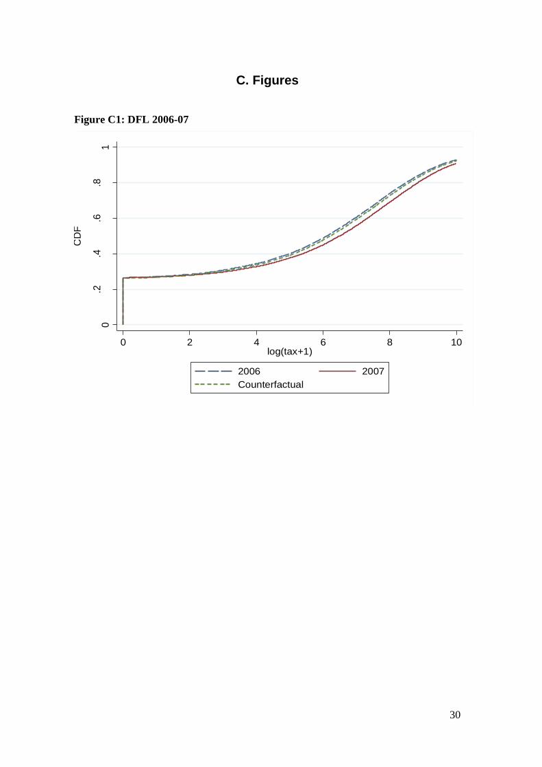
30

C. Figures

Figure C1: DFL 2006-07

0.2

.4.6

.81

CD

F

0 2 4 6 8 10log(tax+1)

2006 2007

Counterfactual

31

Figure C2: Intensive Margin, Quantile Results (logs)

Notes: For our application, regressions in logs underestimate the percentage increase in tax revenue. Log regressions measure the percentage change in taxes between 07 and 06 (where the base is 06) minus the percentage change in taxes between 06 and 05 (where the base is 05). However, 06 should always be used as the base for calculating the percentage change in tax revenue. Given that taxes are smaller in 05 than in 06 logs result in underestimation.

32

References

Abadie, A., (2003), “Semiparametric difference-in-differences Estimators”, Review of

Economic Studies, 72, 1--19.

Albrecht, J., A. Bjorklund and S. Vroman, (2003), “Is There a Glass Ceiling in

Sweden?” Journal of Labor Economics, 21(1), 145-177.

Allingham, M., and A. Sandmo, (1972), “Income Tax Evasion: a Theoretical Analysis,”

Journal of Public Economics, 1, 323–338.

Avi-Yonah, R. and Y. Margalioth (2006), “Taxation in Developing Countries: Some

recent Support and Challenges to the Conventional View”, Unpublished.

Baunsgaard, T. and M. Keen, (2010), “Tax revenue and (or?) trade liberalization,

Journal of Public Economics”, 94(9-10), pages 563-577. October.

Becker, G. (1968), “Crime and Punishment: An Economic Approach,” Journal of

Political Economy, 76, 169.

Boadway, R. and M. Sato, (2009), “Optimal Tax Design and Enforcement with an

Informal Sector,” American Economic Journal: Economic Policy, American

Economic Association, 1(1), pages 1-27, February.

Buchinsky, M. (1994), “Changes in the U.S. Wage Structure 1963-1987: Application of

Quantile Regression” Econometrica, 62 (2), 405-458.

Burgess, R., and N. H. Stern (1993), “Taxation and Development”, Journal of

Economic Literature, 31(2), 762-830.

Carrillo, P. and Yezer, A. (2009), “Alternative Measures of Homeownership Gaps

Across Segregated Neighborhoods,” Regional Science and Urban Economics,

39(5), 542-552.

Central bank of Ecuador (various), Consumer Price Index.

Cowell, F.A. (1990), “Cheating the Government: The Economics of Evasion,” MIT

Press Books, The MIT Press, edition 1, volume 1, number 0262532484, June.

Crocker, K. J. and J. Slemrod (2005), “Corporate tax evasion with agency costs”,

Journal of Public Economics, 89(9-10), pages 1593-1610, September.

Das-Gupta, A. and D. Mookherjee (1998), Incentives and Institutional Reform in Tax

Enforcement. New Delhi: Oxford University Press.

DiNardo, J., Fortin, N., and Lemieux, T. (1996). “Labor market institutions and the

distribution of wages, 1973-1992: A semi-parametric approach”. Econometrica,

64 (5), 1001--1044.

33

Deloitte (2010), “International Tax and Business Guide: Ecuador”.

<http://www.deloitte.com/assets/Dcom-Ecuador/Local%20Assets/Documents/

Doing%20Business%20in%20Ecuador%202008.pdf>

Economist Intelligence Unit, EIU, (Various years), “Ecuador Risk Report”.

<http://www.eiu.com/PublicDefault.aspx>.

Emran, M. S. and S. Farazi, (2009), “Lazy Banks? Government Borrowing and Private

Credit in Developing Countries”, Working Paper, available at SSRN.

Emran. M. S. and J. E. Stiglitz, (2007), “Equity and Efficiency in Tax Reform in

developing Countries”, Working Paper, available at SSRN.

Emran, M. S and J. E Stiglitz, (2005), “On Selective Indirect Tax Reform in

Developing Countries”, Journal of Public Economics, 2005.

Firpo, S. (2007), “Efficient Semiparametric Estimation of Quantile Treatment Effects”.

Econometrica, 75(1), 259-276.

Gordon, R. ed. (2010), Taxation in Developing Countries: Six Case Studies and Policy

Implications, Columbia University Press.

Gordon, R (2010), “Public Finance and Economic Development: Reflections Based on

Experience in China”, Journal of Globalization and Development, Vol. 1, No.1.

Government of Ecuador (2007), “Ley de Regimen Tributario Interno Actualizada”.

Revista Judicial del Ecuador. <http://www.derechoecuador.com/>

Government of Ecuador (2007), “Ley Reformatoria para La Equidad Tributaria en el

Ecuador”. Revista Judicial del Ecuador. <http://www.derechoecuador.com/>

Government of Ecuador (2005), “Codigo Tributario Actualizado”. Revista Judicial del

Ecuador. <http://www.derechoecuador.com/>

Gupta, S., Newberry, K., (1997). “Determinants of the variability in corporate effective

tax rate: Evidence from longitudinal data”. Journal of Accounting and Public

Policy 16, 1–39.

Hanlon, M. and L. Mills and J. Slemrod, (2005), “An Empirical Examination of

Corporate Tax Noncompliance”.

Kim, K., Limpaphayom, P., (1998). “Taxes and firm size in Pacific-Basin emerging

economies”. Journal of International Accounting, Auditing and Taxation 7, 47–

63.

Klepper, S., and D. Nagin, (1989), "The Anatomy of Tax Evasion", Journal of Law,

Economics and Organization, Oxford University Press, 5(1), 1-24.

34

Koenker, R. and Bassett, G. (1978), “Regression Quantiles”, Econometrica, 46(1), 33-

50.

Leibbrandt, M. and J. Levinsohn, and J. McCrary, (2010), “Incomes in South Africa

since the Fall of Apartheid”, Journal of Globalization and Development, Vol 1,

No.1.

Lemieux, T. (2002). “Decomposing Changes in Wage Distributions: A Unified

Approach”. Canadian Journal of Economics, 35 (4), 646-688.

Machado, J. and J. Mata, (2005), “Counterfactual decomposition of changes in wage

distributions using quantile regression,” Journal of Applied Econometrics, 20,

445-465.

MacLaren, J. (2003), “Corruption and the Organization of Tax Administration: Non-

Smithian Benefits from Specialization,” in Institutional Elements of Tax Design

and Reform, Washington: World Bank, 2003.

Mann, A. J. (2004), “Are Semi-Autonomous Revenue Authorities the Answer to Tax

Administration Problems in Developing Countries? A Practical Guide”.

<http://pdf.dec.org/pdf_docs/Pnadc978.pdf>

Mookherjee, D. and P. L. Png, (1994), “Marginal Deterrence in Enforcement of Law”,

Journal of Political Economy, 102(5), pages 1039-66, October.

Nguyen, B., J. Albrecht, S. Vroman, and D. Westbrook, (2007), “A quantile regression

decomposition of urban-rural inequality in Vietnam,” Journal of Development

Economics, 83(2), 466-490.

Polinsky, A. M. and S. Shavell, (2000), “The Economic Theory of Public Enforcement

of Law”, Journal of Economic Literature, American Economic Association, vol.

38(1), pages 45-76, March.

Porcano, T. (1986), “Corporate tax rates: Progressive, proportional, or regressive,”

Journal of the American Taxation Association, 8, 17-31.

Powell, J. (1984). "Least Absolute Deviation Estimation for the Censored Regression

Model," Journal of Econometrics, 25, 303-325.

Rajaraman, I. (2004): “Fiscal Restructuring in the context of Trade Reform”, Economic

and Political Weekly, June 2004.

Rice, E. (1992). “The corporate tax gap: evidence on tax compliance by small

corporations.” In Why People Pay Taxes, edited by Joel Slemrod, 125-61. Ann

Arbor, University of Michigan Press.

35

Saez, E., H. Kleven, M. Knudsen, C. Kreiner, and S. Pedersen, (2010), “Unwilling or

Unable to Cheat? Evidence from a Tax Audit Experiment in Denmark”. Revised

October 2010, forthcoming Econometrica (older version NBER Working Paper

No. 15769, February 2010)

Slemrod, J. and Yitzhaki, S., (2002). Tax avoidance, evasion and administration. In:

Auerbach, A.J., Feldstein, M. (Eds.), Handbook of Public Economics, vol. 3.

Elsevier Science, Amsterdam, pp. 1423-1470, Chapter 22.

Spooner, G.M., (1986). “Effective tax rates from financial statements”. National Tax

Journal 36, 293–306.

Stickney, C., McGee, V., (1982). “Effective corporate tax rates: The effect of size,

capital intensity, leverage and other factors”. Journal of Accounting and Public

Policy 2, 125–152.

Srinivasan, T. N., (1973), “Tax evasion: A model” Journal of Public Economics, 2(4),

pages 339-346.

Stiglitz, J. E (2010), “Development Oriented Tax Policy” in R, Gordon ed. (2010).

Whalley, J. and V. Kononova (2010), “Recent Russian Debate on Moving from VAT to

Sales Taxes and Its Global Implications’, Journal of Globalization and

Development, Vol 1, No.2.

World Bank (2003), “Creating Fiscal Space for Poverty Reduction in Ecuador: A Fiscal

Management and Public Expenditure Review”, World Bank Country Study.

36

Not for Publication: DFL Methodology

To keep our exposition self-contained, we provide a careful description of the

DFL approach using the same notation as in Leibbrandt, Levinshon and McCrary

(2010). Let Y be our variable of interest (log taxes) and 0t and 1t refer to the two

mutually exclusive periods we analyze. The cumulative probability function Y in

period 0t is defined as

dxtTxhtTxyFtTyYtTyF )|(),|(}|Pr{)|( 0000 (1)

Where T is a random variable describing the period from which an observation is

drawn and x is a particular draw of observed attributes of individual characteristics

from a random vector X . ),|( 0tTxyF is the (conditional) cumulative distribution of

Y given that a particular set of attributes x have been picked, and )|( 0tTxh is the

probability density of individual attributes evaluated at x . The cumulative probability

function of Y in period 1t is defined similarly.

Suppose we like to assess how the distribution of Y (taxes) in period 0t (2006)

would look like if the individual attributes x (real-income and assets, for example)

were the same as in period 1t (2007). We denote this counterfactual as 10 ttF and

express it symbolically as59

dxtTxhtTxyFF tt )|(),|( 1010 (2)

In order to compute such counterfactual, Bayes' rule is used to obtain

)(/)|()()|( tTPxXtTPxXPtTxh , and DFL recognized

)(

)(1

)(

)|(1

)|(

)(

)|(

)(

)|(

)|(

)|(10

1

1

1

1

0

0

1

1

0

1 x

tTP

tTP

xXtTP

xXtTP

tTP

xXtTP

tTP

xXtTP

tTxh

tTxhtt

(3)

One may use expression (3) to substitute )|( 1tTxh in equation (1) and obtain

that

dxxtTxhtTxyFyF tttt )()|(),|()(1010 00 (4)

Notice that this expression differs from equation (1) only by )(10

xtt . DFL refer to

59

The subscript “ 10 tt ” indicates that the attributes data from period 0t will be “replaced” by data

from period 1t .

37

)(10

xtt as “weights” that should be applied when computing the counterfactual

distribution of our variable of interest. However, given that the weights are unknown,

they need to be estimated.

To be specific, as in Leibbrandt, Levinshon and McCrary (2009), we summarize

the estimation algorithm for the counterfactual given that a random sample of 0N and

1N observations for periods 0t and 1t is available:

1) Estimate )( 1tTP using the share of observations where 1tTi to obtain

)/()(ˆ1011 NNNtTP i .

2) Estimate )|( 1 xXtTP , by estimating a logit model for both periods. The

dependent variable equals one if 1tTi , and explanatory variables include the vector of

individual attributes ix .

3) For the subsample of observations where 0tTi , estimate the predicted values from

the logit }ˆexp{1

}ˆexp{)|(ˆ

1

i

iii

x

xxXtTP

, where is the parameter vector from the

logit regression. Then, compute the estimated weights as

)(ˆ1

)(ˆ

)|(ˆ1

)|(ˆ

ˆ

1

1

1

1

10

tTP

tTP

xXtTP

xXtTP

i

i

ii

ii

tit

4) For the subsample of observations where 0tTi , compute a weighted empirical

cumulative distribution function. While there are many available options to do this task,

we use the simplest non-parametric option

N

i

tit

N

i

titi

tt

zy

zF

1

1

01

1

01

01

ˆ

ˆ1

)(ˆ

,

where .1 is the indicator function.

It is useful to analyze the differences between the distributions of interest at each

quantile. Specifically, define tTyQ | as the th quantile of the distribution of Y

in period t . Similarly, let 0* | tTyQ be the

th quantile of the counterfactual

distribution of Y if individual attributes where identical to those in 0t and notice that

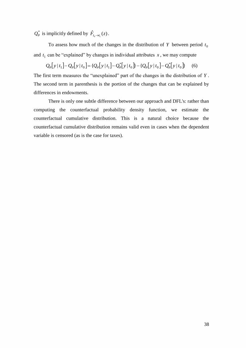
38

*Q is implicitly defined by )(ˆ

10zF tt .

To assess how much of the changes in the distribution of Y between period 0t

and 1t can be “explained” by changes in individual attributes x , we may compute

}||{}||{|| 0*

00*

101 tyQtyQtyQtyQtyQtyQ (6)

The first term measures the “unexplained” part of the changes in the distribution of Y .

The second term in parenthesis is the portion of the changes that can be explained by

differences in endowments.

There is only one subtle difference between our approach and DFL's: rather than

computing the counterfactual probability density function, we estimate the

counterfactual cumulative distribution. This is a natural choice because the

counterfactual cumulative distribution remains valid even in cases when the dependent

variable is censored (as is the case for taxes).