-1-

Tariff and Transport Barriers to Kenyan Trade

Kenyan Chapter Progress Report on EC-PREP Study

Trade Policy and Transport Costs: How EU aid Can Promote Export

Growth in East Africa

By

Jane Kiringai1

Kenya Institute for Public Policy Research and Analysis

Provisional Draft October 2004

1 I acknowledge the research assistance by the KRA Statistics department in availing the relevant trade data. The Research was funded by a grant from Centre of Research in Economic Development and International Trade (CREDIT) of School of Economics, University of Nottingham contracted to KIPPRA. Prof. Morrissey and Rudaheranwa provided insightful comments on earlier drafts all errors and omissions are mine

-2-

1 Introduction Kenya achieved an impressive growth record in the first decade after independence in

the mid to late 1960s. However the growth momentum was not sustained in the 1970s.

ROK( 1975) attributed this slack to three factors, all external sector related; a price

squeeze—in the international markets import prices were rising faster than export

prices; a commodity squeeze—there was a rising trend in imports; and a credit

squeeze—the difficulty of borrowing more from abroad. The only solution—as

identified in the Sessional Paper-- was boosting export performance.

Chart 1.1 Real GDP Growth Rates 1963-2000

Source Analytical Data Compendium (2002)

The trend in chart 1 indicates a steady decline in GDP growth from 1968 to 1974. The

poor performance in 1974 is attributed to the oil shock -- the price of oil increased by

398%. There was a significant improvement in economic growth between 1976 –77,

the coffee boom period recording a growth of 8.3%. However, after the boom an

expansionary fiscal policy was adopted which complicated macroeconomic

management in the medium term. This episode was followed by another sluggish

growth performance between 1984-86 attributed to inter alia balance of payments

problems and droughts. During the period 1978 –1986, the policy response to balance

GDP growth rate

-202468

101214

1964

1966

1968

1970

1972

1974

1976

1978

1980

1982

1984

1986

1988

1990

1992

1994

1996

1998

-3-

of payments problems was increased controls, items would be shifted to more

restrictive import control schedules followed by relaxation once the situation

improved, resulting in a complex structure of protection. During the same period East

Asian countries that had opened up and liberalised their trade regimes achieved high

growth rates. Empirical evidence pointed to a strong relationship between growth and

export performance and by early 1990s the empirical evidence on the benefits of trade

liberalization was convincing and it is on such evidence that trade liberalization was

predicated.

Trade reforms in Kenya started in the early 1990s. The outward orientation strategy

was characterized by trade and commercial policy reforms intended to introduce

efficiency gains in the economy by eliminating distortions and ‘getting the prices

right’ through a greater reliance on markets. Quantitative restrictions were replaced

with tariffs; average tariffs were lowered and made more uniform. Trade policy

reforms were complemented by liberalization of the exchange rate and additional

export incentives also aimed at increasing external competitiveness.

A decade later trade liberalization has not delivered the promise of high real growth

rates, export performance has been sluggish, economic growth has witnessed a

consistently declining trend since 1996. Population growth rate has been well above

the growth rate of productive output, resulting in rising poverty and unemployment.

During the recession period population growth averaged 2.8% while economic growth

averaged about 2.4%, the corollary is a gradual decline in incomes per capita. In terms

of contribution to national output, agriculture maintains the lead accounting for 24%

of GDP, the manufacturing sector has not matured to emerge as the principle export

sector as was initially envisaged under the infant industry thesis.

This study seeks to analyse the post liberalisation structure of protection in Kenya,

from 1990 to 2000. Using the partial equilibrium approach, Effective Protection

Coefficients, (EPCs), will be computed at industry/activity level and ranked to

determine the direction of resource pulls in production. The EPCs will be used to

compare the rates of protection across industries and across time to uncover the

impact of trade liberalisation on the structure of protection in Kenya. Further, the

-4-

study will analyse the structure of protection arising from transport costs as a natural

barrier to trade.

The rest of the paper is organised as follows; section two is background covering

trade performance and policy regimes in Kenya. Effective rates of protection from

tariffs are computed and discussed in section three. Protection and taxation arising

from international freight costs and domestic transport costs are covered in section

four. The summary and conclusions are covered in section five.

2 Trade Regimes in Kenya

2.1 Background

The poor performance of the external sector has been the motivation behind several

liberalisation2 episodes identified for the Kenyan economy, see for instance Reinikka

(1994), Maxwell Stamp Associates (1989) Glenday and Ndii (2003). Though there is

no consensus on the exact timing of the liberalisation episodes, the periodic increase

in imports of goods and services (episodes 1-8 in chart 2) appear to coincide with the

analytically derived episodes. Reinikka (1994), for instance, identifies five episodes;

the first such attempt was in 1973 following the oil shock—a 398% increase in the

price of oil leaving the country in a severe foreign exchange crunch-- but was not

sustainable. Exchange controls had to be tightened to conserve foreign exchange,

reversing the measures instituted in 1973. The second episode followed the coffee

boom 1976-77, the higher earnings from coffee relaxed the foreign exchange

constraint. The policy response was to relax import restrictions.

The period between the first and second liberalisation episodes was characterized by

persistent balance of payments deficits. The four fold OPEC oil price increase in 1974

combined with a 5% increase in the domestic demand for crude petroleum per annum

between 1974 and 1980 exacerbated the balance of payment problems. By 1979 120%

of coffee export earnings were required to pay for oil imports, (ROK 1980). During

the same period the plan to achieve an 8% increase in the growth of exports was not

realizable, and there was a fall in the price of agricultural commodities in the

2 Trade liberalisation is defined as the reduction in quantitative restrictions and replacement with tariffs and the subsequent reduction and unification of tariffs

-5-

international market. Furthermore, as a result of the break up of the East African

Community, (EAC) in 1977, Kenya lost the Tanzanian market which was an

important destination for her exports.

Chart 2.1 Foreign trade as % of GDP

0.0%

5.0%

10.0%

15.0%

20.0%

25.0%

30.0%

35.0%

40.0%

45.0%

1964

1966

1968

1970

1972

1974

1976

1978

1980

1982

1984

1986

1988

1990

1992

1994

1996

1998

2000

Expts Impts

1 2 3

4 5 6

78

Source KIPPRA data Compendium

The third liberalisation episode was motivated by the need to correct macroeconomic

imbalances, the aftermath of the expansionary fiscal policy, which followed the coffee

boom. Between the three liberalisation episodes, the BOP deficit increased and each

crisis would be addressed through ad hoc quantitive restrictions in addition to the

existing tariffs. Export performance deteriorated and the need to remove the anti

export bias in the trade policy regime became the overriding concern which was

addressed through the import substitution strategy.

The stated policies under the IS strategy were; to contain the growth of imports to less

than 2% on annual basis down from 7.3%, increase the growth of exports to 8% per

annum and stimulate domestic production in substitution for imports and to support

exports. Oil imports for non-essential services were to be taxed at a higher rate to

contain the growth of imports. Other non-essential imports were to be contained

through higher sales taxes together with quantitive restrictions on the same and

exemptions when deemed necessary. An export subsidy of 10% on manufactured

-6-

goods to promote exports; a foreign exchange allocation committee was constituted

and an export import licensing office opened to manage the controls, all aimed at at

increasing exports. The corollary was that a complex structure of protection emerged,

characterised by tariff escalation and redundancy; the scope for discretion and the

rents from quantitive restrictions created a fertile environment for rent seeking

activities.

Though the controls reduced the volume and value of imports from 39% as as a share

of GDP in 1980 to 27.6% in 1984, reducing the BOP deficit, trade performance

deteriorated. Import controls constrained the growth of manufacturing and export

potential; exports averaged 25% of GDP during this period. When the IS strategy was

adopted during the second half of 1980s, GDP growth rate ranged between 4-6% but,

like elsewhere in the world, the strategy was unsustainable. The growth of

manufacturing emanated mainly from domestic demand and once the demand was

saturated the scope for growth under IS was limited. Following the failure of IS

strategy, Kenya started implementing a gradual liberalisation programme in 1986—

with specific focus of eliminating anti export bias.

2.2 Recent Developments

The tariff rationalisation programme started in 1986 with policy pronouncements in

ROK (1986) and the National Development Plans. Trade policy reforms comprised of

three components; rationalize the tariff code, reduce the average tariff rates and

reduce the number of tariff bands (Pritchett and Sethi 1994). Kenya has been

undertaking trade reforms since the early 1990s, both as part of conditionality and

also through preferential trade arrangements. Starting from 1990 there has been a

gradual reduction in both the tariff rates—with special focus on imported

intermediate inputs-- and tariff bands . The magnitude of reduction is constrained by

revenue loss implications and the gradual pace allows for reforms to shift to other

sources of revenue.

Duty rates on imported raw materials and spare parts were targeted for reduction so as

to reduce the anti export bias and improve the country’s competitiveness. Duty rates

for this category of goods ranged between 10% and 100% in 1990— the first steps in

-7-

the liberalisation process were to reduce tariffs on intermediate inputs by an average

of 5%, while increasing duty on finished products by a maximum of 35%. Duty on

capital equipment and parts has also been targeted for reduction in the liberalisation

process, and items taxed at 3% and 5% were zero rated by 2003. A similar reduction

was applied to raw materials that are not produced locally.

The other liberalisation measure has been the reduction in the number of tariff bands.

Starting from 1989, the number of tariff categories was reduced from 25 to 17,

abolishing eight rates –55%,65%, 75%, 90%, 95%, 110 %, 125% and 170%. In 1990

another five categories were eliminated, reducing the bands to 12. A further

compression in 1992 reduced the bands to 11 and to 9 by 1993. Currently there are

four tariff bands, free, 5%, 15%, 25% and 35%. Over a decade, the number of rates

was reduced from twenty five to five, and the maximum rate from 170% to 35%.

In the liberalisation process, 1993 presented specific challenges, and there was a 25%

temporary increase in duty rates. This was occasioned by the high inflationary

pressure in the domestic markets and the mopping up exercise significantly increased

domestic interest payments, additional revenues had to be mobilised through tariff

revenue to cover the additional expenditure.

With the exception of specific agricultural commodities, notably sugar—the tariff

liberalisation has resulted in a significant reduction in tariff barriers. The top rate has

been capped at 35%. However, there have been notable policy reversals; duty on

fabrics was raised from 25% to 35%, to protect local producers, duty on locally

available food stuffs was raised to 35% while the duty on other sugar increased to

100%. The duty rates applied on wheat and sugar imports from COMESA constitute a

trade dispute among the trading partners. Overall with eight tariff bands and a top rate

of 35%, the IMF rates the Kenyan trade regime at 6%, on a scale of 1-103, a

moderately restrictive trade policy (IMF 2003).

3 scale 10 represents the most restrictive trade regime

-8-

2.3 Export Performance

A review of export performance indicates that there are only two episodes when

Kenya recorded a balance of payments surplus (chart 2). The first was during the

coffee boom in 1977, thereafter the country witnessed several years of declining terms

of trade. The second episode of a balance of payments surplus was recorded in 1993-

94--during this period growth in exports recorded a 14% increase in value terms. A

combination of a weak shilling, abolition of exchange controls and a fall in the real

wage resulted in a significant increase in export earnings (Glenday and Ndii 2000),

however the high level of export growth was not sustained.

Three principal measures were put in place to introduce an export bias after

liberalisation; duty/VAT remission—Export Promotion Programmes Office, Export

Processing Zones ( EPZ) and Manufacturing Under Bond (MUB). In addition,

regional trade agreements under COMESA and EAC are also intended to enhance

export performance. These measures were intended to increase the share of

manufactured exports (services were also included later) as a share of total exports

following the fall of prices of primary commodities in the international market

resulting in adverse terms of trade for the country.

Under the export compensation scheme, exporters were to claim 10% of the value of

their exports based on the f.o.b value. The findings from a manufacturing survey

undertaken in the late 1970s indicated that only 37% of the exporting firms claimed

to have increased exports as a result of export compensation, 40% of the firms

considered the subsidy as a windfall gain and did not change their exporting

decisions, a further 16% did not claim the subsidy (Low 1982). Analysts argue that

delays and uncertainty in administration of the scheme reduced the true value of the

subsidy. ERP estimates during this period (Low 1982), indicate that the 10% subsidy

was not sufficient to remove the anti export bias. Food, beverages and tobacco

industries, for instance, required a subsidy of 40% to remove the anti export bias,

within these activities tinned peeled tomatoes required, a subsidy of 85.44% to have a

neutral regime and for paper packaging 60.64%. Increasing the subsidy to 20% in

1980 did not effectively eliminate the implicit taxes on most of the commodities.

-9-

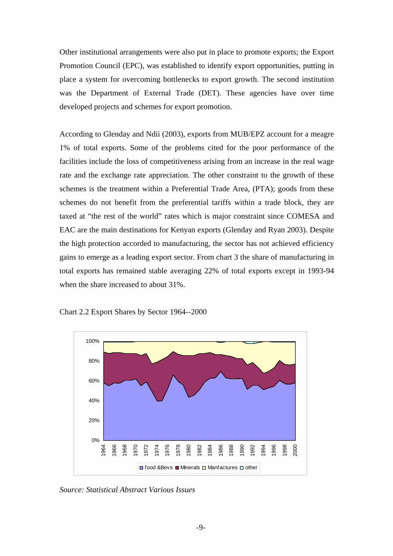
Other institutional arrangements were also put in place to promote exports; the Export

Promotion Council (EPC), was established to identify export opportunities, putting in

place a system for overcoming bottlenecks to export growth. The second institution

was the Department of External Trade (DET). These agencies have over time

developed projects and schemes for export promotion.

According to Glenday and Ndii (2003), exports from MUB/EPZ account for a meagre

1% of total exports. Some of the problems cited for the poor performance of the

facilities include the loss of competitiveness arising from an increase in the real wage

rate and the exchange rate appreciation. The other constraint to the growth of these

schemes is the treatment within a Preferential Trade Area, (PTA); goods from these

schemes do not benefit from the preferential tariffs within a trade block, they are

taxed at “the rest of the world” rates which is major constraint since COMESA and

EAC are the main destinations for Kenyan exports (Glenday and Ryan 2003). Despite

the high protection accorded to manufacturing, the sector has not achieved efficiency

gains to emerge as a leading export sector. From chart 3 the share of manufacturing in

total exports has remained stable averaging 22% of total exports except in 1993-94

when the share increased to about 31%.

Chart 2.2 Export Shares by Sector 1964--2000

Source: Statistical Abstract Various Issues

0%

20%

40%

60%

80%

100%

1964

1966

1968

1970

1972

1974

1976

1978

1980

1982

1984

1986

1988

1990

1992

1994

1996

1998

2000

food &Bevs Minerals Manfactures other

-10-

In Kenya agriculture continues to be the principle sector four decades after

independence. Furthermore, despite being the leading sector, agriculture itself has not

done well. Indeed, excluding coffee and tea, all other exports as a share of GDP fell

from 14% in the period 1962-71, 13 % in 1972 - 80, 8% over1981- 1992 but

recovered to 13.2% in 1993-1998. By the year 2002, coffee tea and horticulture

accounted for 53% of total export earnings despite price decline in the international

markets for primary commodities (especially coffee).

Africa continues to be the dominant export market for Kenyan goods accounting for

49% of total exports in 2002, followed by Western Europe and Asia each accounting

for 28% and 15% respectively. Of the 49% share destined for the African market,

55% is accounted for by Uganda and Tanzania. Europe takes the lead as the origin for

imports accounting for 34% of total imports, Africa accounts for only 11% of total

Kenyan imports. Imports from COMESA and EAC, thus comprise a small component

of total imports. From the trading pattern, the formation of a customs union within the

two trading blocks will have a significant impact on the structure of protection in the

partner countries, as key importers from Kenya, while the corresponding impact for

Kenya will be determined by the magnitude of reduction of current tariff levels to the

agreed Common External Tariff, CET.

For the COMESA region, the proposed CET of 0, 5, 15 and 25% for capital goods,

raw materials, intermediate goods and final goods respectively, is currently under

revision by the COMESA secretariat to achieve a customs union by 2004. Under the

EAC Customs Union, goods from Uganda and Tanzania are to be imported into

Kenya duty free. The EAC protocol established a three band CET, 0% for raw

materials 10 % for intermediate goods and 25% for all finished goods. When the CET

becomes effective in 2005, it will ultimately change the structure of protection in

Kenya. The 26-35% tariff rates, for instance, will collapse to 25%, reducing the

current top rate from 35 to 25% and reducing the tariff bands from eight to three.

-11-

3 Analytical Framework There are two approaches to evaluating the structure of protection; these are the

partial equilibrium approach and the computable general equilibrium approach. Some

of the partial equilibrium measures commonly used include the nominal rate of

protection, (NRP), effective rate of protection, (ERP), Trade Restrictiveness Index ,

TRI, and the index of implied import restrictiveness (IIIR). While nominal tariffs

influence consumer behaviour through the price raising effect, effective protection

influences production by pulling resources from sectors with low ERPs ( and non

tradeable goods sectors) to sectors with High ERPs. The ERP, is the percentage

increase in value added per unit in economic activity permitted by the tariff structure,

holding the exchange rate constant. It can be defined as the ratio of domestic to world

value added, relative to a non interventionist trade regime, (Corden 1966;Anderson

1996 ; Conway and Bale 1988).

Effective protection takes into account three effects; the share of value added in final

output, tariffs on intermediate inputs and tariffs on final output. Effective protection

thus measures the magnitude of implicit taxation of value added. The measure can be

insightful and has revealed cases of negative value added--even for profitable

industries-- tariff escalation and negative effective protection, (Greenaway and Milner

2003; Anderson 2003). Perhaps more important for a country like Kenya that has

adopted an outward orientation aimed at promoting exports, ERP can reveal

incidences of anti export bias since exports do not benefit from a tariff on final goods

like import competing products.

Once the coefficients are computed at industry level, the relative magnitudes indicate

the direction of resource pulls. On the production side, the resources will be drawn out

of industries with low effective protection to industries with high rates of protection.

On the absorption side, there will be substitution from goods with high nominal tariffs

to goods with low tariffs.

The works of Balassa (1965), Johnson (1965) and Corden (1966) Basevi (1966) are

perhaps some of the earliest in both theory and empirical evidence of effective

-12-

protection. Algebraically, EPC can be derived as follows; (see for instance Corden

1966; Greenaway and Milner 1993))

Value added for activity j in the absence of a tariff can be expressed as

)1( ijjv app −= (2)

If a tariff tj is levied on the final output of activity j and ti levied on the intermediate

input used in the activity then value added for activity j after tariffs is given by:

)]1()1[('iijjjv tatpp +−+= (3)

The change in value added as a result of the intervention is derived by netting (2)

from (3);

v

vvj p

ppe −=

'

(3)

[ ]et a t p a

p ajj ij i j ij

j ij

=+ − + − −

−

( ) ( ) ( )( )

1 1 11

(4)

which reduces to:

ij

iijjj a

tate

−−

=1

(5)

In a case where there are many inputs in the production of j (i= 1,2,…..n), the

weighted average of input tariffs is used in place of the single input tariff, thus (5)

becomes

∑

∑

−

−= n

ij

n

iiijj

j

a

tate

11

(6)

Where Pv is the value added per unit of good j at free trade prices and pv’ is the value

added per unit of j at tariff distorted prices, tj is the nominal tariff levied on industry j,

aij is the share of final value added of j accounted for by input i and ti is the nominal

tariff levied on intermediate input i. The aij are the technical coefficients derived from

the input output table. Equation [6] does not incorporate non traded inputs which can

-13-

introduce a bias in the computed coefficients. To adjust for non traded inputs model

[6] Balassa (1962) approach will be adopted;

∑ ∑

∑

−−

−= n

mmjij

n

iiijj

j

aa

tate

11

[7]

where amj are the technical coefficients for non traded inputs.

3.2 Data and Methodology Equation [6] will be used to compute the effective protection coefficients. The data

requirements for the model are the aij (technical coefficients from the input output

table), ti (nominal tariffs on intermediate inputs) and tj (nominal tariffs on the final

product j). The choice of nominal tariff depends on data availability. One option is the

implicit tariff, computed as tariff revenue as a proportion of import value before

tariffs. The second option is using the legal tariff as published in the tariff schedule.

However, the later can bias the ERP estimates as it does not take into account

exemptions. For the purpose of this study- the implicit tariff will be used as the

nominal rate of protection.

Trade data is obtained from the Kenya Revenue Authority at eight digit SITC level

and aggregated to three digit level then mapped to the Input Output table sector level.

Tariffs tj are computed at the input output table sector level, while the ti are computed

by weighting the tj by the technical coefficients. The mapping between input output

table sectors and the three digit SITC is presented in Annex 4.

The Input output tables provide the technical coefficients aij. The unpublished 1990

update will be used to compute ERP for the years 1990 and 1994. This version of the

input output table will be updated to 1997 and used to compute ERPs for the years

1997 and 2000. The tables are disaggregated into domestic and imported intermediate

inputs, reported in producer prices and are therefore duty inclusive. The coefficients

from the table are therefore post-protection technical coefficients.

-14-

The post-protection technical coefficients have to be deflated to generate the adjusted

technical coefficients in terms of free trade (border) prices. To transform the

coefficients to border prices the Balassa et al (1982), method is used, given by the

expression:

aijw

)1()1(

i

j

tt

++

= aij [9]

relating the post-protection (aij) and free trade (aijw) input-output coefficients in which

tj and ti are tariff rates on final output and inputs respectively. Tariffs imposed on

inputs would discourage the production of j (thus reduced output) and therefore

aij>aijw while tariffs on output would encourage production of output j thus aij< aij

w

and would be given by the following relationship

aij1990 = )1)1(

1990

1990

j

i

tt

++

aijw. [10]

In transforming the input-output coefficients for the production of nontraded inputs, ti

is assumed to equal zero because the Balassa method is employed, which assumes

there is no distortion in production of nontraded goods. The deflated coefficients are

used in the estimation of ERPs for all the other years.

3.3 RESULTS The results by sector are presented in table 3.1. From the results we classify the

industries into four clusters; industries that have been disprotected throughout,

industries that have enjoyed positive protection before and after liberalisation;

industries that were protected but are now disprotected—the losers. The fourth

category are industries that were disprotected before liberalisation but now enjoy

positive levels of protection—the gainers.

In the first category are beverages and tobacco industries where the magnitude of

disprotection has been declining over time from -36.44 to -2.7 in the year 2000.

However, the negative rates for beverages and tobacco reflect infinite protection

rather than negative protection, where ∑− ija1 is negative (see annex 9). Petroleum

based industries fall into this category, the level of discrimination has declined over

time from -1.2 at the onset of liberalisation to -0.11 by the year 2000. The

-15-

disprotection for manufacture of metallic products has witnessed a gradual decline

from -0.63 to -0.35 between 1990 and 2000.

Table 3.1 Nominal and Effective rates of Protection

NRP ERP 1997_table

Sector 1990 1994 1997 2000 1990 1994 1997 2000 1997b 2000b

1 Traditional economy 0.00 0.00 0.00 0.00 0.00 0.00 0.00 0.00 0.00 0.002 Agriculture 0.05 0.03 0.18 0.19 0.04 0.02 0.19 0.20 0.19 0.20 3 Fishing and Forestry 0.32 0.02 0.06 0.07 0.32 -0.02 0.06 0.07 0.06 0.07 4 Mining and Quarrying 0.06 0.11 0.11 0.10 -0.19 -0.11 0.16 0.16 0.18 0.17 5 Mfg . Food prep's 0.05 0.16 0.13 0.17 -0.43 0.50 0.23 0.60 0.16 0.40 6 Mfg . Bakery prod's 0.59 0.15 0.19 0.21 11.87 -0.01 1.65 1.26 0.11- 0.07- 7 Mfg . Bev & Tobacco 0.65 0.20 0.15 0.15 -36.44 -0.62 -3.83 -2.70 0.21 0.17 8 Mfg . Raw Textiles 0.13 0.15 0.05 0.08 0.13 0.16 0.02 0.07 0.05- 0.18 9 Mfg . Finished Textiles 0.27 0.26 0.14 0.15 0.40 0.38 0.25 0.25 2.38 2.41 10 Mfg . Clothing 0.07 0.20 0.30 0.41 -0.27 0.51 1.44 2.10 1.17 1.70 11 mfg . Leather & Footwear 0.22 0.23 0.23 0.23 0.97 0.79 1.00 0.94 0.67 0.63 12 Mfg . Wood prod's 0.28 0.21 0.21 0.18 0.28 0.00 0.55 0.46 0.35 0.29 13 Mfg . Paper print & publ 0.09 0.02 0.06 0.06 0.07 -0.05 0.09 0.08 0.08 0.08 14 Mfg . Petroleum prod's 0.69 0.89 0.16 0.13 -1.20 -1.64 -0.15 -0.11 0.17- 0.12- 15 Mfg . Rubber prod's 0.19 0.21 0.15 0.15 0.25 0.29 0.31 0.31 0.26 0.26 16 Mfg . Paint Det & soap 0.11 0.06 0.06 0.05 0.14 -0.29 -0.08 -0.21 0.05- 0.16- 17Mfg . Other chemicals 0.18 0.11 0.05 0.05 0.58 -0.01 -0.21 -0.25 0.08- 0.11- 18 Mfg . Non Metal min prod's 0.23 0.03 0.13 0.11 -0.13 -1.08 0.22 0.21 0.15 0.15 19 Mfg . Met prod's & mach 0.15 0.06 0.12 0.10 -0.63 -0.41 -0.40 -0.35 0.42- 0.36- AVE 0.23 0.16 0.13 0.14 -1.28 -0.08 0.08 0.16 0.26 0.31 1997b and 2000b Rates are computed from a 1997 input output table updated by the author from the 1990 Table.

Alternative Table:

-16-

Sector 1990-1994 1997-2000 1990-1994 1997-2000 1997-2000b

7 Mfg . Bev & Tobacco 0.43 0.15 -18.53 -3.26 0.1919 Mfg . Met prod's & mach 0.10 0.11 -0.52 -0.38 -0.39 17Mfg . Other chemicals 0.14 0.05 0.29 -0.23 -0.1016 Mfg . Paint Det & soap 0.08 0.06 -0.08 -0.15 -0.1114 Mfg . Petroleum prod's 0.79 0.14 -1.42 -0.13 -0.141 Traditional economy 0.00 0.00 0.00 0.00 0.008 Mfg . Raw Textiles 0.14 0.07 0.14 0.05 0.073 Fishing and Forestry 0.17 0.07 0.15 0.06 0.0713 Mfg . Paper print & publ 0.06 0.06 0.01 0.08 0.084 Mining and Quarrying 0.09 0.11 -0.15 0.16 0.182 Agriculture 0.04 0.19 0.03 0.20 0.1918 Mfg . Non Metal min prod's 0.13 0.12 -0.61 0.21 0.159 Mfg . Finished Textiles 0.27 0.15 0.39 0.25 2.4015 Mfg . Rubber prod's 0.20 0.15 0.27 0.31 0.265 Mfg . Food prep's 0.10 0.15 0.04 0.42 0.2812 Mfg . Wood prod's 0.24 0.19 0.14 0.50 0.3211 mfg . Leather & Footwear 0.22 0.23 0.88 0.97 0.656 Mfg . Bakery prod's 0.37 0.20 5.93 1.45 -0.0910 Mfg . Clothing 0.13 0.36 0.12 1.77 1.44AVE 0.20 0.13 -0.68 0.12 0.29

Average NRP Average ERP

In the second category is agriculture, manufacture of bakery products, raw and

finished textiles, leather and footwear, wood products and rubber industries. In this

group of industries the general trend is a marginal increase in the level of effective

protection. The industries that have gained from liberalisation (from negative to

positive rates of protection) include non metallic mineral industries, clothing and

textile industries and mining and quarrying. The industries that enjoy the highest level

of protection are clothing and textiles followed by manufacture of bakery products.

The results are presented in table 3.1

Effective rates of protection give a broad indication of the direction of resources pulls

within the economy. From the results, it would be expected that within the tradeable

goods sector there would be a shift in resources towards manufacture of bakery

products and clothing and textiles industries which enjoy a high component of

assisted value added. From the analysis two losers emerge; paints detergents and soap

industries and other chemical industries.

-17-

Within the partial equilibrium approach there are two methods for measuring ERPS—

industrial survey approach and the Input Output table approach. In Kenya both of

these approaches have been used and as would be expected with remarkably different

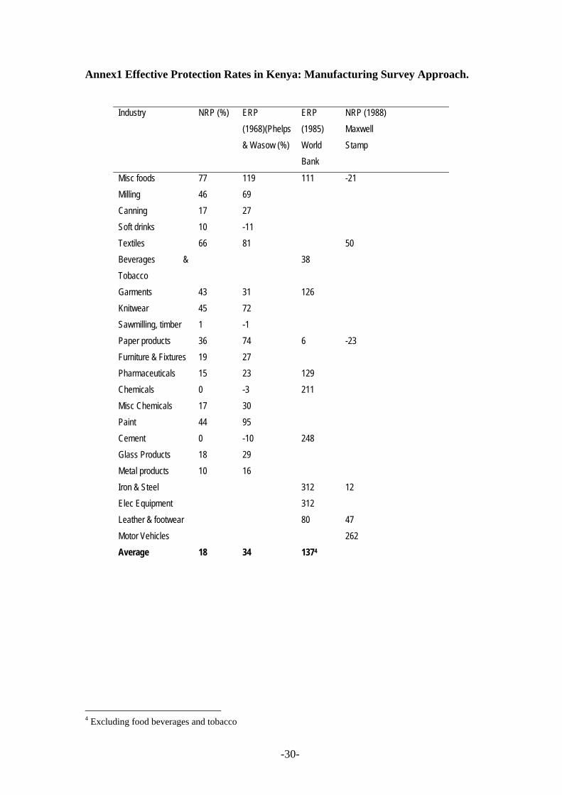
results. Phelps and Wasow (1968), Maxwell Stamp Associates(1988) and the World

Bank (1987a) used the industrial survey approach while Keyfitz and Wanjala (1991)

and Damus and Eugene (1989) used the input output table approach. (see annexes 1 &

2).

The emerging evidence from these studies is that during the 1980s manufacturing

enjoyed a high component of assisted value added, that service sectors had negative

ERPs, and that agricultural sector had very low levels of protection. The resource

pulls would therefore be away from service sectors and agriculture to manufacturing.

Since agriculture was and still remains the main export sector, the structure of

protection thus created an anti export bias, drawing resources to a sector that was

producing inefficiently behind protective barriers.

Phelps and Wasow (1968) computed an ERP ranging between –78% for

confectionary and 173% for sugar while the nominal rate varied between 0% and

77%. From the World Bank study the ERPs ranged between 312% for iron and steel

and 6% for paper and wood products. The differences in the findings are attributed to

timing, sample size and selection and the level of aggregation. The changes in other

offsetting effects are difficult to disentangle to make direct comparisons.

Damus and Beaulieu (1989) computed ERPs for five years 1967, 1971, 1976,1981

and 1986. The main finding from this study was that most manufacturing sectors were

heavily protected while agriculture had low levels of protection. Service sectors had

negative protection, a finding attributed to the import substitution strategy being

implemented during this period. According to the study manufactured food was

accorded the highest level of protection 665% followed by beverages and tobacco

with an ERP of 555%. Further the trend indicated a significant increase in effective

protection between 1967 and 1986.

The findings by Keyfitz and Wanjala (1991) were broadly in tandem with those of

Damus and Beaulieu (1989), the rates varied between dis-protection of –31.3% for

-18-

restaurants and hotels to 855.5% for beverages and tobacco.(see annex for more

details ). The other sectors with high ERPs included food processing, raw textiles,

paints detergents and soap with ERPS of 527.9%, 141.7% and 162.4% respectively.

Most of the service sectors had negative ERPs which was attributed to the tariffs

levied on petroleum products a key input in the sectors while the negative ERPs for

restaurants was attributed to the high protection in foods and beverages which are the

key inputs for this sector. The high ERPs for paints is attributable to high nominal

tariffs in the sector itself.

3.4 The Impact of EAC Customs Union

In this section the impact of the EAC Customs union is simulated. The EAC customs

will become effective in year 2005; the three countries will have a common external

tariff rate system 0% for raw materials, 10% for semi finished goods and a maximum

tariff of 25% for all finished products. Since the tariff bands in Kenya are higher than

the CET rates and even compared to the other EAC countries (Uganda’s top rate is

15%), it is expected that the implementation of the protocol will significantly reduce

the tariff barriers.

The simulations are based on the same model but instead of using the actual tariff as

computed above, tj becomes the scheduled CET of 25% while ti takes the value 0%

and 10% scheduled rates. The results are compared with a shift from the current

scheduled top rate of 35%.

The results are presented in the table 3.2 are therefore based on 35%, and 25% NRP

and the respective ERPs. The findings indicate that the protective barriers will

gradually decline from an average of 12% to about 3% when the EAC protocol

becomes effective. This compares favourably with an average of 16% for the year

2000, (table 3.1) based on the actual tariff. The other interesting observation is that

the ERP computed from the scheduled tariff is 12% while using the actual tariff the

ERP is 16% showing that using the scheduled tariff understates the ERP, in this case

with 4 percentage points.

-19-

Table 3.2 EAC Customs Union Simulations NRP ERP Sector 2000 2005 2000 2005

(25%) 2005 (10%)

1 Traditional economy 0.00 0.00 0.00 0.00 0 2 Agriculture 35.00 25.00 0.36 0.26 0.102381 3 Fishing and Forestry 35.00 25.00 0.36 0.25 0.101694 4 Mining and Quarrying 35.00 25.00 0.58 0.41 0.164378 5 Mfg . Food prep's 35.00 25.00 0.96 0.69 0.274947 6 Mfg . Bakery prod's 35.00 25.00 0.70 0.50 0.200289 7 Mfg . Bev & Tobacco 35.00 25.00 -6.11 -4.36 -1.74506 8 Mfg . Raw Textiles 35.00 25.00 0.44 0.31 0.125226 9 Mfg . Finished Textiles 35.00 25.00 0.49 0.35 0.139606 10 Mfg . Clothing 35.00 25.00 1.16 0.83 0.331997 11 mfg . Leather & Footwear 35.00 25.00 0.65 0.46 0.185035 12 Mfg . Wood prod's 35.00 25.00 0.66 0.47 0.189242 13 Mfg . Paper print & publ 35.00 25.00 0.55 0.40 0.158307 14 Mfg . Petroleum prod's 35.00 25.00 -0.16 -0.11 -0.04521 15 Mfg . Rubber prod's 35.00 25.00 0.64 0.46 0.182382 16 Mfg . Paint Det & soap 35.00 25.00 0.50 0.36 0.142466 17Mfg . Other chemicals 35.00 25.00 0.97 0.69 0.277869 18 Mfg . Non Metal min prod's 35.00 25.00 0.66 0.47 0.188933 19 Mfg . Met prod's & mach 35.00 25.00 -1.17 -0.84 -0.33498 AVE 33.16 23.68 0.12 0.08 0.03

4 Transport Costs Transport costs are a natural barrier to trade. Effective rates of protection arising from

transport costs are analysed relative to a situation where there are no transport costs.

Several studies (Amjadi and Yeats 1995, Yeats 1994) for instance argue that transport

costs are more detrimental to African export competitiveness than tariff barriers and

account for the decline in Africa’s share in world trade. In 1990/91 transport costs

accounted for 15% value of the regions exports (Amjadi and Yeats 1995).

Through Africanization, most government own airlines and shipping lines, a process

that has led to cartelized international freight, increasing transport costs for the region

-20-

reducing export competitiveness. By 1991 estimates, freight and insurance costs

translated to 15% of export earnings, compared to 6% for developed countries,

(Collier and Gunning 1999). The findings indicate that rail transport costs are double

the rates in other regions.

In Kenya the ad valorem freight rates for some sectors are even higher than those

cited by Amjadi and Yeats (1995). In the horticulture sector in Kenya for instance,

transport costs are cited as one of the key challenges to competitiveness. In rose

marketing transport to market accounts for 68.9% of total costs translating to Kshs

6.16 per stem; estimating the price of a stem at Kshs. 17 in the international market

then the transport component translates to an ad valorem rate of 35% or an implicit

tax of 35%. For coffee, transport costs account for 6.7% of the value for small

holders through the cooperative and 6.2% for large plantations.

Bulk transportation in Kenya is handled between Kenya Railways and private trucks.

The Railway network operates on a two rates system, up direction from Mombassa to

the mainland and down direction from the mainland to the port. The up direction rates

are higher than the down direction rates reflecting the demand pattern determined by

the Kenyan pattern of trade; there is a higher tonnage of imports to be ferried in the up

direction than the exports in the down direction. Furthermore, the competition from

roads is much stiffer in the down direction, the trucks usually have no tonnage after

delivering imports and they charge very low rates for downward bound cargo and thus

drive down the down direction rates even for railway. There are often interested in

covering their fuel costs since 70% of the down direction traffic is empty trucks.

This pattern of trade is also reflected in the lead times of container clearance at the

Mombasa port. The table shows that on average it takes 4 days to clear an outward

bound container both 20ft and 40ft compared to 9-10 days for inward bound

containers. Further the findings from a recent growth and competitiveness report

(World Bank 2004) indicate that customs procedures are another source of delay and

informal payments by freight forwarders are used to accelerate the process. The

evidence from the report indicates that a “vessel delay surcharge” compounds the

problems at the port for importers.

-21-

Table 4.1 Clearing of Container Average (No of days)

OUTWARD CLEARING INWARD CLEARING

2002 2001 2002 2001 COST ($)

20 ft 4 7 10 18 1174 40 ft 4 8 9 19 2112

Source: World Bank/KIPPRA RPED Survey, 2003 The rail line has two corridors to Uganda, the southern corridor through Kisumu and

the Northern corridor through Malaba. The southern corridor is a more efficient route

because of the Wagon ferry service over Lake Victoria, through this corridor it is

possible to transfer wagons from rail to ferry. However, the axle limit to 36 metric

tonnes along the Nakuru—Kisumu route constrains the potential of a profitable route.

The northern corridor Mombasa- Malaba- Kampala which has a higher axle load limit

poses specific challenges; the rates within Uganda, Malaba –Kampala are very high to

the extent they deter potential users of the line. Indeed some transporters use the line

to Malaba and then switch to trucks which again reduce efficiency through

transhipment and double handling.

In determining the transport tariffs other transporters use the rail rates as a benchmark

for transporting cargo in the upward direction. Though the railway system has a

higher capacity, the major disadvantage is inefficiency in transit times due to lack of

door to door delivery. Since the major industries do not have warehouses along the

railway line, the option entails transhipment and double handling—from wagons to

trucks and from trucks to warehouse, this increases costs lead time in delivery.

Between 1990 and 1996-2000 the tonnage moved by Kenya railways declined 3.1

Million metric tonnes to 1.6 metric tonnes. Approximately 30% of the cargo handled

at the Mombassa port is carried via the railway network, in the year 2002/03 for

instance Kenya Railways ferried 2.3 million tonnes of cargo. After a period of low

tonnage, the railway system is regaining its position as a key transporter following the

implementation of axle load limits for trucks, the high capacity of the rail then makes

it a more efficient option.

-22-

4.1 Data and Methodology

In this case, the effective rate of protection is the percentage change in value added

per unit as a result of freight costs relative to the situation in the absence of such costs.

To quantify the impact of international freight costs, equation [7] is modified as

follows:

∑

∑

−

−= n

ij

n

iiijj

j

a

dad

11

η [8].

Where dj and di be the ad valorem freight rates borne on output j and input i

respectively and aij is as defined in [1].

Domestic transport costs explicitly tax domestic producers. Transport cost on final

output and inputs jointly compound the magnitude of taxation. To estimate the

effective implicit taxation model [8] will be adjusted to take into account the

compounding effect of transport costs on inputs.

∑

∑

−

+= n

ij

n

iiijj

j

a

dad

11

η [9]

The international freight rates dj and di are computed using data from the Kenya

Revenue Authority (KRA). The data is obtained at 8 digit level SITC. Before

aggregating to three digit all entries where freight data—freight and insurance-- is not

provided are dropped from the sample reduce the bias from data. The remaining

entries are aggregated to three digit and the ad valorem freight rate computed as the

difference between the C.I.F value F.O.B value divided by the C. I.F value.

j

jjj c

fcd

−= [10]

where cj and fj are the C.I.F and F.O.B values for industry j respectively, di is

computed by weighting the dj by the deflated technical coefficients.

-23-

The internal transport costs are computed based on the scheduled railway tariff for the

years 1993, 2001 ad 2003. The choice of the railway tariff is based on anecdotal

evidence that other transporters benchmark their rates on the Kenya Railways rates,

the computed rates can therefore be perceived as a floor. The Kenya Railways

schedule gives the rate per tonne per kilometre, the total transport charges therefore

depend on the distance hauled.

To estimate the ad valorem transport rate export unit prices are obtained from the

customs data set, the unit prices are used to estimate the ton value for each

commodity. The transport cost per ton is divided by the ton value and multiplied by

the distance. In the absence of accurate distance covered for each commodity we use

the distance between Nairobi and Mombasa as an average, the estimates are thus

conservative.

4.2 Results

4.2.1 International Freight Implicit protection of domestic producers arising from international freight rates

reflects an overall reduction in effective rates of protection. Compared to a high 700%

for bakery products in 1990, the highest in 2000 was 29% for clothing and textile

industries and forestry and fishing. The results are presented in table 4.2. The results

are presented as two year averages to smooth the data, 1990 and 1994 and 1997 and

2000. The results reflect an overall decline in the ad valorem transport costs from

23% when liberalisation started in early 1990s to 11% by the year 2000. However, the

protection of value added remains high reflecting a seven percentage point decline

from 29% to 22% during the period. This shows that although policy induced barriers

(tariffs) have reduced the level of protection, natural protection via transport costs

remain high. The implication is that intra region trade or ‘south south’ trade where

transport costs are not prohibitive holds a high of potential. On the other hand if

Kenya has to diversify to north south trade international freight rates have to be

reduced significantly, one option is increasing exports to match the imports tonnage.

-24-

Table 4.2 Protection Arising From International Freight Transport Costs

Sector 1990-94 1997-2000 1990-94 1997-2000

1 Traditional economy 0.00 0.00 0.00 0.002 Agriculture 0.24 0.11 0.24 0.113 Fishing and Forestry 0.20 0.22 0.21 0.244 Mining and Quarrying 0.30 0.19 0.56 0.485 Mfg . Food prep's 0.17 0.10 0.12 0.196 Mfg . Bakery prod's 0.31 0.08 3.62 0.087 Mfg . Bev & Tobacco 0.16 0.16 -2.21 0.318 Mfg . Raw Textiles 0.17 0.13 0.20 0.659 Mfg . Finished Textiles 0.18 0.07 -0.07 0.4810 Mfg . Clothing 0.19 0.17 0.52 0.7511 mfg . Leather & Footwear 0.29 0.10 0.99 0.1712 Mfg . Wood prod's 0.19 0.11 0.23 0.1713 Mfg . Paper print & publ 0.20 0.10 0.28 0.1514 Mfg . Petroleum prod's 0.19 0.05 0.14 0.1215 Mfg . Rubber prod's 0.25 0.08 0.40 0.1416 Mfg . Paint Det & soap 0.15 0.08 0.12 0.05 17Mfg . Other chemicals 0.21 0.11 0.36 0.2218 Mfg . Non Metal min prod's 0.53 0.11 1.09 0.2119 Mfg . Met prod's & mach 0.43 0.10 -1.36 -0.34Average 0.23 0.11 0.29 0.22

NRP ERP

4.2 Implicit Export Taxation through Domestic Transport costs

The average nominal rate in the early 1990s was 14% very close to the rates cited by

Collier and Gunning (1999). The rates have declined significantly estimated at 7%

mainly due to liberalisation and competition. However when the technology of

production is taken into account to transport cost on inputs, the effective taxation

remains high. From an average of 49% in 1993 the effective implicit taxation is

declined to 31% in 2001 and to 20% by 2003. Again it is important to pint out that the

rates are computed based on the railway scheduled tariff and based on a Nairobi

Mombasa distance so the rates are based on a conservative estimate and could be even

higher than computed in this study. The high rates of taxation coupled with other

domestic transaction costs reduce the competitiveness of Kenyan exports.

-25-

Table 4.3 Implicit Taxation from Domestic Transport Costs

Sector 1993 2001 2003 1993 2001 2003

1 Traditional economy - - - 2 Agriculture 0.18 0.13 0.09 0.21 0.15 0.10 3 Fishing and Forestry 0.01 0.01 0.01 0.02 0.01 0.01 4 Mining and Quarrying 0.62 0.46 0.29 0.94 0.72 0.45 5 Mfg . Food prep's 0.07 0.05 0.03 0.78 0.52 0.33 7 Mfg . Bev & Tobacco 0.14 0.10 0.06 0.86 0.32 0.21 8 Mfg . Raw Textiles 0.06 0.04 0.03 0.14 0.17 0.11 9 Mfg . Finished Textiles 0.06 0.04 0.03 0.13 0.15 0.10 10 Mfg . Clothing 0.19 0.14 0.09 0.43 0.30 0.19 11 mfg . Leather & Footwear 0.01 0.01 0.01 0.31 0.19 0.12 13 Mfg . Paper print & publ 0.14 0.11 0.07 0.45 0.32 0.21 14 Mfg . Petroleum prod's 0.03 0.02 0.01 1.47 1.02 0.65 15 Mfg . Rubber prod's 0.07 0.05 0.03 0.28 0.19 0.12 16 Mfg . Paint Det & soap 0.23 0.17 0.11 0.87 0.59 0.38 17Mfg . Other chemicals 0.11 0.08 0.05 0.58 0.36 0.23 18 Mfg . Non Metal min prod's 0.06 0.03 0.02 19 Mfg . Met prod's & mach 0.18 0.13 0.09 0.83 0.23 0.15 AVE 0.14 0.10 0.07 0.49 0.31 0.20

NRP ERP

5 summary and conclusion The influence of trade policy on growth performance introduces a paradox in the

structure of protection for an economy in the process of development. On one hand

there was a perceived need to protect infant industries—perceived as a road map to

industrialisation through high tariffs and non-tariff barriers, while generating the

much needed revenue for the government. On the other hand the price raising effect

even for intermediate inputs and the distortions created by the protective barriers

increase inefficiency in the domestic market particularly in manufacturing and

agriculture reducing their competitive potential and the growth prospects envisaged.

This paradox is clearly reflected in the effective structure of protection in Kenya.

Ideally trade liberalisation is intended to increase the price of exportables relative to

importables to switch production in favour of exports away from import competing

goods. The price incentive is also intended to constrain domestic demand to increase

-26-

the scope for exports. However the outcomes from policy changes are at best

unpredictable particularly given the other policy changes which may lead to

conflicting signals, the most import one in this case being the exchange rate policy

which might inadvertently reverse the trade policy intent.

International freight costs form a natural barrier to trade; assuming the costs computed

in this study are borne by the neighbouring countries in the same magnitude, then the

neighbouring countries form a captive market for the country that emerges as a

competitive producer, even when tariff barriers are removed under WTO or Economic

Partnership agreements. Indeed as more industrial country in the EAC block, Kenya

should seek to increase efficiency in production to ensure she retains the captive

market. However high internal transport costs threaten the competitiveness of Kenyan

producers; improving the road and railway network, enhancing reforms in Kenya

Railways and are some of the measures that are necessary to give Kenya a

competitive edge. Increasing export cargo at Mombasa port to even out inward bound

and outward bound cargo would also reduces inefficiency and lead times at the port.

From the analysis above, it is evident that though nominal tariffs have been

significantly reduced, the structure of protection for some sectors is still negative.

Though the magnitude may vary depending on the methodology and approach, the

results nevertheless point to the intricacies in the structure of protection, where the

outcomes depend not just on the nominal tariffs but also on the production

technology.

The estimation of the true structure of protection poses a number of challenges. First,

trade policy is not the responsibility of a single ministry or agency. In Kenya the

policies cut across the ministries of Finance, Trade/ Commerce and Industries

(depending on the period in question) and sometimes even the Agriculture Ministry.

Tracing and quantifying the impact of trade policy across all the agencies then

becomes a Herculean task. The second challenge is that new measures are introduced

in ad hoc manner during crisis and remain in place even after the crisis is over. Some

of these ad hoc measures are evident from table 1 especially after the oil crisis, which

resulted in the foreign exchange crunch in mid 1970s.

-27-

An examination of Annex3 shows the complexity of determining the actual outcome

of trade policy. A look at the export and import policy indicates a complex mix of

import substitution and export promotion. Furthermore the price incentive in the tariff

structure dictates that consumers switch to the consumption of non tradeables despite

the policy intent. Clearly, isolating the net impact of trade policy is not a straight

forward exercise. Indeed the analysis overlooks the rent seeking activity associated

with protection.

The third challenge is in the underlying assumption that input output coefficients are

fixed, that the elasticities of demand for exports and the supply of imports are infinite,

that all tradeable goods remain traded even after tariffs are levied and that fiscal and

monetary policies maintain internal balance and finally the non existence of non

traded inputs in the production of j. Clearly, the input output coefficients are not fixed

in the medium term to long term and can introduce a bias in the estimate coefficients.

Despite these weaknesses and challenges, EPC continue to be widely used as it gives

policy makers insights into the direction of resource pulls without the complex

simulations. The findings from this study thus give a general direction of resource

pulls within the Kenyan economy.

-28-

References

Amjadi A. and Yeats A. (1995) “Have Transport Costs Contributed to the relative decline of Sub-Saharan Exports?: Some preliminary empirical evidence” Policy Research Working Paper No 1559, World Bank, Washington DC.

Balassa B. (1988) “Incentive Policies and Agricultural Performance in Sub-Saharan

Africa” Working paper No 77, The World Bank. Balassa, B., and Associates (1982), Development Strategies in Semi-industrial

economies, A World Bank Research Publication, The Johns Hopkins University Press

Collier, P. and Gunning, J. (1999) ‘Explaining African economic performance’,

Journal of Economic Literature, Vol. 37 (March), pp. 64–111, 1999 Conway P. and Bale M. (1988) “ Approximating the Effective Protection Coefficient

without Reference to Technological Data” The World Bank Economic Review, Vol 2, No 3: 349-363.

Corden M. (1966) “ The Structure of a Tariff System and the Effective Protective

rate” The Journal of Political economy, Vol 74, No. 3 (Jun., 1966), 221-237. Corden M. (1975) “ The costs and Consequences of Protection: A survey of Empirical

Work” in Kenen B> ed International trade and Finance Cambridge University Press.

Damus S. and Beaulieu E. (1989) “ Effective Protection in Kenya” Technical Paper

No. 89-13, Ministry of Planning and National Development. Glenday G. and Ryan T.C. (2003) “Trade Liberalization and Economic Growth in

Kenya” in Kimenyi M. Mbaku J. and Mwanikiki N. eds Restarting and Sustaining Economic Growth and Development in Africa: The Kenya Case. Ashgate Publishing

Glenday G. and Ndii D. (2003) “ Export Platforms in Kenya” in Kimenyi M. Mbaku

J. and Mwaniki N. eds Restarting and Sustaining Economic Growth and Development in Africa: The Kenya Case. Ashgate Publishing

Greenaway D. (1993) “ Liberalising through Rose-Tinted Glasses” The Economic

Journal , Vol. 103, No. 416 (Jan. 1993) 208-222. Greenaway, D. and Milner C.R. (1995), Trade and Industrial Policy in Developing

Countries ( London MacMillan) Hertel T., Ivanic M., Preckel P. And Cranfield J. (2003) “Trade Liberalisation and the

Structure of Poverty in Developing Countries” Global Trade Analysis Project (GTAP)

-29-

Keyfitz R. and Wanjala J. (1991) “Optimal Tariff Reform for Kenya” Technical Paper 91-05, Ministry of Planning and National Development

Kruger A., Schiff M., and Valdes A., (1988) “Agricultural Incentives in Developing

Countries: Measuring the Effect of Sectoral and Economy wide policies “ The World Bank Economic Review , Vol 2, No. 3:255-271

Low P. (1982) “Export Subsidies and Trade Policy: The experience of Kenya.” World

Development, Vol. 10, No. 4, pp. 293-304, 1982 Milner C. (1995) “Discovering the Truth About Protection Rackets” Inaugural lecture

presented at the University of Nottingham Tuesday 21 November, 1995. Oyejide T., (1992) “Effects of Trade and Macroeconomic Policy on African

Agriculture” in Schiff M. and Valdes eds, The political economy of agricultural pricing policy Volume 4 A synthesis of Developing countries A word bank comparative study, John Hopkins University Press.

Pritchett L., and Sethi G., (1994) “Tariff Rates, Tariff Revenue and Tariff Reform:

Some new Facts” The World Bank Economic Review , Vol 8, No. 1:1-16. Reinikka R. (1994) “ How to Identify Trade liberalisation Episodes in Kenya: An

Empirical Study on Kenya” Centre for the Study of African Economies WPS/94-10, University of Oxford.

ROK Statistical Abstract Various Issues. ROK (1975) Sessional Paper No. 4 of 1975 on Economic Prospects and Policies ROK (1980) Sessional Paper No.4 of 1980 on Economic Prospects and Policies. Taylor L.(1993) “The Rocky Road to Reform” in Taylor L ed The Rocky Road to

reform: Adjustment , Income Distribution and Growth in the Developing World MIT Press Cambridge, Massachusetts.

World Bank (2004) “Growth and Competitiveness in Kenya” World Bank Africa

Region, Private Sector Division.

-30-

Annex1 Effective Protection Rates in Kenya: Manufacturing Survey Approach.

Industry NRP (%) ERP

(1968)(Phelps & Wasow (%)

ERP (1985) World Bank

NRP (1988) Maxwell Stamp

Misc foods 77 119 111 -21 Milling 46 69 Canning 17 27 Soft drinks 10 -11 Textiles 66 81 50 Beverages & Tobacco

38

Garments 43 31 126 Knitwear 45 72 Sawmilling, timber 1 -1 Paper products 36 74 6 -23 Furniture & Fixtures 19 27 Pharmaceuticals 15 23 129 Chemicals 0 -3 211 Misc Chemicals 17 30 Paint 44 95 Cement 0 -10 248 Glass Products 18 29 Metal products 10 16 Iron & Steel 312 12 Elec Equipment 312 Leather & footwear 80 47 Motor Vehicles 262 Average 18 34 1374

4 Excluding food beverages and tobacco

-31-

Annex 2 Effective Protection Coefficients for Kenya5

5 D&B refers to Damus and Beaulieu (1989) while K & W refers to Keyfitz and Wanjala (1991)

Effective Protection Rates for KenyaD & G K & W

1976 1981 1986 1986Traditional Economy -1.5 -3.3 -2.3 -2.3Agriculture 3.2 2.4 1.7 13Forestry and Fishing 13 25.5 10.2 12.6Mining and Quarrying 59.1 -23.8 -34.2 64Mfg. Food Processing 79.4 71.7 665 527.9Mfg. Bakery Products 62.1 687 65.5 67.9Mfg. Bev. & Tobacco 222 319 555 855.5Mfg. Raw Textiles 65.5 62.3 118 141.7Mfg. Finished textiles 96.8 136 70.3 83.4Mfg. Clothing 102.1 -0.2 16.5 22.1Mfg. Leather 200 103 74.9 90.7Mfg. Wood Products 30.2 133 27.4 68.7Mfg.Paper Products 22.7 17 29.7 38.8Mfg. Petroleum -46.3 16.3 -159 44.4Mfg. Rubber products 18.3 49.1 41.8 51.6Mfg. Paint Detergents 78.7 189 121 162.4Mfg. Other Chemicals 9.7 38.1 3.9 15Mfg. Non Metals 43.4 431 -12.1 120.8Mfg. Metallic Products 17.9 25.1 19.9 32.9Repair of Transport Equipmen 57.9 32.8 4.3 14.1Electricity -5.8 -9.7 -22.8 -9.9Water -2.9 -6.4 -10.7 -5.5construction -17.4 -22.6 -28.9 -18.2Trade -1.2 -3.1 -5.6 -3Transportation -10 -10.3 -23.7 -11.4 Communications -7.2 -5.8 -6 -5.8Restraustrants & Hotels -25.5 -27.1 -32.6 -31.3Ownership of Dwellings 0 0 0 0Financial Services -0.6 -1.5 -1.9 -1.2Non Govt Services -6 10.5 240 -6.4Govt Public Admin -2.8 -6.2 -11.5 -6.5Govt Education -1.5 -2.5 -4 -1.6ovt Health -3.2 -6.5 -8.2 -7.6Govt Agricultrure -5.1 -9.2 -19.1 -7.6Govt Other -2.9 -6.6 -10.2 -8.8

mean 65.72Std. Deviation 167.99

-32-

Annex 3 Some Important Trade Policy Episodes

Period Imports Exports 1963-1970

High growth rates

Customs agreement between

Uganda Tanzania and Kenya

with a common tariff and the

use of quantitive restrictions.

Exchange controls on sterling

transactions . exchange

controls become a

responsibility of CBK

Measures to eliminate the

import of goods made in

Kenya.

1970-1974

A 398% increase in the

price of oil --extreme loss

of foreign reserves.

Import bans, quotas and

licenses introduced. Exchange

control approvals required—

369 items under restriction,

150 items banned 147 items

on quota.

Imports over Kshs 2000

require forex license.

1974-1980

Tighter controls

Contain the growth of imports

to 25 on annual basis and.

Import demand to be curbed

through quantitive restrictions

and high taxes. Import

substitution strategy –as

measure to contain import

demand. Import deposit

Scheme introduced

Increase the growth of exports by

8% per annum

Export growth encouraged through

an export subsidy of 10 % on

manufactured goods with at least

30% value added.

Marketing boards formed for

marketing of all exports of coffee,

tea, cotton and horticulture.

1980 –1985

SAL by world Bank aims:

Reduced protection,

devaluation &market lib.

Export insurance scheme

• Replace quantitive

restrictions with tariffs.

• Forex allocation

committee & Import

export licensing office to

administer controls

Eliminate the IS bias against exports.

Export promotion measures:

• Export credit and guarantee

scheme

• Simplify export compensation

scheme for approved categories

-33-

• Imports of finished goods

deleted from GPCO

• Import Management

committee (IMC) formed

Transparency through

publication of 3 import

schedules (I IIA & IIB)

of exports

• Export compensation raised to

20%

1986 – 1990

Import Substitution

Processing charge for import

application increased from 1%

to 1.5% (value +freight)

Introduction of manufacture Under

Bond--MUB

1991 –1995

full liberalisation

Removal of forex controls

replacement of QRs by tariffs

and tariff rationalisation

• COMESA free Trade Area

• Export Processing Zone bill

• MUB VAT zero rated

1996-2000 Export compensation reduced from

20% to 18%

Annex 4. Mapping 3digit SITC to Input Output Table Sectors

-34-

-35-

Annex 5 1990 Trade Data Kshs Million

I-O Sec qty fob cif cust_val duty salestax tariff 1 tariff2 tariff 3 tariff 42 611.0 648 1,350 4,590 73 2 5% 5% 2% 2%3 10.3 0 1 442 0 0 48% 32% 0% 0%4 511.0 300 403 1,220 27 15 7% 6% 2% 2%5 379.0 1,450 1,800 3,910 100 46 6% 5% 3% 2%6 0.4 0 0 11 1 0 146% 59% 5% 5%7 293.0 48 61 11,100 116 84 190% 65% 1% 1%8 32.0 14 16 424 2 0 15% 13% 1% 1%9 21.7 541 668 1,190 249 62 37% 27% 21% 17%

10 11.1 160 301 339 23 10 8% 7% 7% 6%11 17.1 38 56 713 16 9 28% 22% 2% 2%12 159.0 629 722 1,160 274 39 38% 28% 24% 19%13 8.2 471 420 680 40 21 9% 9% 6% 5%14 1,890.0 192 307 7,740 689 3,430 224% 69% 9% 8%15 21.5 505 496 530 120 132 24% 19% 23% 18%16 27.8 1,560 1,640 2,250 195 41 12% 11% 9% 8%17 319.0 3,230 3,690 4,630 804 170 22% 18% 17% 15%18 481.0 1,840 2,080 3,170 606 277 29% 23% 19% 16%19 409.0 15,100 18,400 28,600 3,130 1,460 17% 15% 11% 10%21 0.2 36 60 62 6 3 10% 9% 10% 9%

Total 26,762 32,471 72,761 6,470 5,800

tariff 1 duty/ C.I.F valuetariff 2 duty/ (C.I.F value +duty)tariff 3 duty/ (customs value )tariff 4 duty/ (customs value +duty)

-36-

Annex 6 Computation of 1990 Freight Rates

I-O Sec fob cif qty cust_val duty salestax CIF-FOB Rate1 rate22 583 687 100 677 66 2 104.10 18% 15%3 0 0 0 0 0 0 0.03 17% 15%4 286 373 167 370 19 10 86.90 30% 23%5 964 1,158 127 1,146 94 45 193.80 20% 17%6 0 0 0 0 0 0 0.04 89% 47%7 89 111 2 103 16 2 21.76 24% 20%8 14 16 2 16 2 - 2.04 15% 13%9 719 930 14 840 107 30 211.50 29% 23%

10 172 204 5 147 9 3 31.70 18% 16%11 34 55 2 38 11 6 20.27 59% 37%12 601 723 36 690 142 20 122.30 20% 17%13 353 421 6 380 19 10 68.50 19% 16%14 1,713 2,274 1,200 4,828 16 6 561.00 33% 25%15 402 468 16 357 78 110 66.40 17% 14%16 1,292 1,508 7 1,386 111 24 216.00 17% 14%17 3,257 3,882 260 3,817 587 125 625.00 19% 16%18 1,595 1,884 60 1,593 328 145 289.00 18% 15%19 14,060 16,440 207 15,230 1,019 502 2,380.00 17% 14%21 37 43 0 39 5 2 5.89 16% 14%

Rate 1 (cif-fob)/fobRate 2 (cif-fob)/cif

-37-

Annex 7 Trade Distorted Coefficients matrixSectors TRADCONAGRIC FOFISH MINE MANFD BAKE BEVS RAWTEX FINTEX CLOTH FTWEAR WOODPROD

1 TRADCON 0.061 0.000 0.000 0.000 0.000 0.000 0.000 0.000 0.000 0.000 0.000 0.0002 AGRIC 0.000 0.023 0.000 0.000 0.223 0.001 0.011 0.107 0.000 0.005 0.032 0.0003 FOFISH 0.027 0.000 0.001 0.000 0.002 0.000 0.000 0.000 0.000 0.000 0.000 0.0474 MINE 0.000 0.000 0.000 0.000 0.000 0.000 0.000 0.000 0.000 0.000 0.000 0.0005 MANFD 0.000 0.013 0.000 0.000 0.386 0.582 0.269 0.000 0.000 0.000 0.310 0.0006 BAKE 0.000 0.000 0.000 0.000 0.001 0.000 0.000 0.000 0.000 0.000 0.000 0.0007 BEVS 0.000 0.000 0.000 0.000 0.000 0.000 0.062 0.000 0.000 0.000 0.000 0.0008 RAWTEX 0.000 0.006 0.014 0.018 0.005 0.000 0.000 0.042 0.107 0.002 0.001 0.0089 FINTEX 0.000 0.000 0.000 0.000 0.000 0.000 0.000 0.000 0.051 0.290 0.014 0.008

10 CLOTH 0.000 0.004 0.000 0.000 0.000 0.000 0.000 0.000 0.000 0.040 0.000 0.00011 FTWEAR 0.000 0.000 0.000 0.000 0.000 0.000 0.000 0.000 0.000 0.000 0.050 0.00012 WOODPROD 0.021 0.000 0.000 0.001 0.000 0.000 0.001 0.000 0.000 0.000 0.000 0.10713 PPUB 0.000 0.000 0.000 0.014 0.042 0.006 0.018 0.007 0.011 0.043 0.058 0.00314 PTROL 0.000 0.010 0.046 0.260 0.075 0.013 0.117 0.080 0.067 0.060 0.025 0.25415 RUBBER 0.000 0.001 0.002 0.006 0.002 0.000 0.003 0.000 0.000 0.002 0.107 0.00816 PDSOAP 0.000 0.000 0.000 0.000 0.000 0.000 0.000 0.000 0.000 0.000 0.000 0.00317 CHEMCS 0.000 0.031 0.000 0.014 0.031 0.001 0.015 0.017 0.091 0.009 0.074 0.02518 NONMET 0.065 0.000 0.000 0.081 0.004 0.002 0.024 0.002 0.001 0.001 0.000 0.00619 METALICS 0.026 0.004 0.000 0.039 0.066 0.002 0.042 0.065 0.027 0.086 0.025 0.11420 REPEQP 0.000 0.001 0.011 0.049 0.014 0.003 0.018 0.010 0.005 0.019 0.004 0.05021 ELEC 0.000 0.004 0.000 0.005 0.005 0.001 0.005 0.007 0.010 0.006 0.006 0.00322 WATER 0.000 0.000 0.000 0.003 0.001 0.001 0.009 0.000 0.005 0.001 0.000 0.00023 CONSTC 0.000 0.000 0.000 0.003 0.001 0.000 0.001 0.000 0.000 0.001 0.000 0.00124 TRADE 0.005 0.013 0.001 0.013 0.041 0.003 0.043 0.022 0.029 0.070 0.030 0.03325 TRANSP 0.000 0.002 0.000 0.049 0.010 0.000 0.020 0.002 0.002 0.002 0.001 0.00526 COMMUNC 0.000 0.000 0.000 0.001 0.003 0.000 0.003 0.005 0.006 0.009 0.001 0.00327 RESTHOT 0.000 0.000 0.000 0.000 0.000 0.000 0.000 0.000 0.000 0.001 0.000 0.00028 DWELL 0.000 0.000 0.000 0.000 0.000 0.000 0.000 0.000 0.000 0.000 0.000 0.00029 FINSERV 0.000 0.000 0.000 0.053 0.036 0.006 0.035 0.062 0.072 0.175 0.011 0.05630 NONGVTSERV 0.000 0.000 0.000 0.017 0.005 0.001 0.008 0.002 0.005 0.010 0.018 0.00531 PADMIN 0.000 0.000 0.000 0.000 0.000 0.000 0.000 0.000 0.000 0.000 0.000 0.00032 GOVEDU 0.000 0.000 0.000 0.000 0.000 0.000 0.005 0.000 0.000 0.000 0.000 0.00033 GOVHET 0.000 0.000 0.000 0.000 0.000 0.000 0.000 0.000 0.000 0.000 0.000 0.00034 GOVAGR 0.000 0.000 0.000 0.000 0.000 0.000 0.000 0.000 0.000 0.000 0.000 0.00035 GOVOT 0.000 0.000 0.000 0.000 0.000 0.000 0.000 0.000 0.000 0.000 0.000 0.00036 OTH 0.000 0.000 0.000 0.059 0.007 0.014 0.005 0.012 0.009 0.057 0.021 0.015

-38-

Annex 8 Trade Free (Deflated) Coefficients matrix

Sectors Ad valorem TarTRADCONAGRIC FOFISH MINE MANFD BAKE BEVS RAWTEX FINTEX CLOTH FTWEAR WOODPRODPPUB1 0.00 0.061 0.000 0.000 0.000 0.000 0.000 0.000 0.000 0.000 0.000 0.000 0.000 0.0002 0.05 0.000 0.023 0.000 0.000 0.224 0.001 0.018 0.116 0.000 0.006 0.037 0.000 0.0003 0.32 0.020 0.000 0.001 0.000 0.001 0.000 0.000 0.000 0.000 0.000 0.000 0.046 0.0004 0.06 0.000 0.000 0.000 0.000 0.000 0.000 0.000 0.000 0.000 0.000 0.000 0.000 0.0005 0.05 0.000 0.013 0.000 0.000 0.386 0.881 0.423 0.000 0.000 0.000 0.359 0.000 0.0006 0.59 0.000 0.000 0.000 0.000 0.001 0.000 0.000 0.000 0.000 0.000 0.000 0.000 0.0007 0.65 0.000 0.000 0.000 0.000 0.000 0.000 0.062 0.000 0.000 0.000 0.000 0.000 0.0008 0.13 0.000 0.005 0.016 0.017 0.004 0.000 0.000 0.042 0.120 0.002 0.001 0.010 0.0019 0.27 0.000 0.000 0.000 0.000 0.000 0.000 0.000 0.000 0.051 0.245 0.013 0.008 0.00110 0.07 0.000 0.004 0.000 0.000 0.000 0.000 0.000 0.000 0.000 0.040 0.000 0.000 0.00011 0.22 0.000 0.000 0.000 0.000 0.000 0.000 0.000 0.000 0.000 0.000 0.050 0.000 0.00012 0.28 0.016 0.000 0.000 0.001 0.000 0.000 0.002 0.000 0.000 0.000 0.000 0.107 0.00013 0.09 0.000 0.000 0.000 0.014 0.040 0.008 0.028 0.008 0.013 0.042 0.065 0.004 0.41614 0.69 0.000 0.006 0.036 0.163 0.047 0.013 0.115 0.053 0.050 0.038 0.018 0.191 0.02415 0.19 0.000 0.001 0.002 0.006 0.001 0.000 0.004 0.000 0.000 0.002 0.110 0.008 0.00116 0.11 0.000 0.000 0.000 0.000 0.000 0.000 0.000 0.000 0.000 0.000 0.000 0.003 0.00017 0.18 0.000 0.028 0.000 0.013 0.028 0.002 0.021 0.017 0.098 0.008 0.077 0.027 0.03018 0.23 0.053 0.000 0.000 0.070 0.004 0.002 0.033 0.002 0.001 0.001 0.000 0.006 0.00019 0.15 0.022 0.004 0.000 0.036 0.061 0.003 0.061 0.064 0.030 0.080 0.026 0.127 0.04620 0.00 0.000 0.001 0.014 0.052 0.014 0.005 0.029 0.011 0.006 0.020 0.005 0.064 0.01021 0.10 0.000 0.004 0.000 0.005 0.005 0.001 0.007 0.008 0.011 0.006 0.006 0.004 0.00322 0.00 0.000 0.000 0.000 0.003 0.001 0.001 0.014 0.000 0.006 0.001 0.000 0.000 0.00023 0.00 0.000 0.000 0.000 0.003 0.001 0.000 0.001 0.000 0.000 0.001 0.000 0.001 0.00224 0.00 0.005 0.014 0.002 0.014 0.043 0.005 0.071 0.025 0.036 0.075 0.037 0.042 0.03725 0.00 0.000 0.002 0.000 0.052 0.011 0.000 0.032 0.003 0.003 0.003 0.002 0.006 0.00826 0.00 0.000 0.000 0.000 0.001 0.004 0.000 0.005 0.006 0.008 0.009 0.002 0.004 0.01527 0.00 0.000 0.000 0.000 0.000 0.000 0.000 0.000 0.000 0.000 0.001 0.000 0.000 0.00028 0.00 0.000 0.000 0.000 0.000 0.000 0.000 0.000 0.000 0.000 0.000 0.000 0.000 0.00029 0.00 0.000 0.000 0.000 0.056 0.037 0.009 0.057 0.071 0.092 0.187 0.013 0.071 0.06630 0.00 0.000 0.000 0.000 0.018 0.005 0.001 0.013 0.003 0.006 0.011 0.022 0.006 0.01331 0.00 0.000 0.000 0.000 0.000 0.000 0.000 0.000 0.000 0.000 0.000 0.000 0.000 0.00032 0.00 0.000 0.000 0.000 0.000 0.000 0.000 0.008 0.000 0.000 0.000 0.000 0.000 0.00033 0.00 0.000 0.000 0.000 0.000 0.000 0.000 0.000 0.000 0.000 0.000 0.000 0.000 0.00034 0.00 0.000 0.000 0.000 0.000 0.000 0.000 0.000 0.000 0.000 0.000 0.000 0.000 0.00035 0.00 0.000 0.000 0.000 0.000 0.000 0.000 0.000 0.000 0.000 0.000 0.000 0.000 0.00036 0.00 0.000 0.000 0.000 0.063 0.008 0.023 0.008 0.014 0.011 0.061 0.025 0.019 0.022

-39-

Annex 9 Computing 1990 ERP

aijtiSectors Ad valorem TarTRADCONAGRIC FOFISH MINE MANFD BAKE BEVS RAWTEX FINTEX CLOTH FTWEAR WOODPRODPPUB

1 0.00 - - - - - - - - - - - - - 2 0.05 - 0.001 - - 0.011 0.000 0.001 0.006 - 0.000 0.002 - - 3 0.32 0.007 - 0.000 - 0.000 - - - - - - 0.015 - 4 0.06 - - - - 0.000 - - - - - - - - 5 0.05 - 0.001 - - 0.020 0.046 0.022 - - - 0.019 - - 6 0.59 - - - - 0.000 - - - - - - - - 7 0.65 - - - - - - 0.041 - - - - - - 8 0.13 - 0.001 0.002 0.002 0.001 - - 0.006 0.016 0.000 0.000 0.001 0.000 9 0.27 - - - - - - - - 0.014 0.066 0.004 0.002 0.000 10 0.07 - 0.000 - - 0.000 - - - - 0.003 - - - 11 0.22 - - - - 0.000 - - - - - 0.011 - - 12 0.28 0.004 - - 0.000 0.000 - 0.001 - - - - 0.030 0.000 13 0.09 - 0.000 - 0.001 0.003 0.001 0.002 0.001 0.001 0.004 0.006 0.000 0.036 14 0.69 - 0.004 0.025 0.113 0.032 0.009 0.079 0.037 0.035 0.026 0.012 0.132 0.017 15 0.19 - 0.000 0.000 0.001 0.000 0.000 0.001 - - 0.000 0.021 0.002 0.000 16 0.11 - - - - 0.000 - - - - - - 0.000 - 17 0.18 - 0.005 - 0.002 0.005 0.000 0.004 0.003 0.017 0.001 0.014 0.005 0.005 18 0.23 0.012 - - 0.016 0.001 0.000 0.007 0.001 0.000 0.000 - 0.001 0.000 19 0.15 0.003 0.001 - 0.005 0.009 0.000 0.009 0.009 0.004 0.012 0.004 0.018 0.007

tj - sum(aijti) 0.04 0.30 0.08- 0.03- 0.54 0.49 0.07 0.18 0.04- 0.13 0.07 0.02

1- sum(aij)-sum(mj) 0.895 0.929 0.414 0.074 0.045 -0.013 0.557 0.456 0.162 0.132 0.245 0.303

Ej 0.04 0.32 0.19- 0.43- 11.87 36.44- 0.13 0.40 0.27- 0.97 0.28 0.07