Tableaux for Distributed Temporal Logic · Tableaux for Distributed Temporal Logic Applications to Security Protocols Joana Margarida Simões de Abreu Dissertação para a obtenção

Tableaux for Distributed Temporal LogicApplications to Security Protocols

Joana Margarida Simões de Abreu

Dissertação para a obtenção de Grau de Mestre em

Matemática e Aplicações

Júri

Presidente: Professora Doutora Cristina Sales Viana Serôdio SernadasOrientador: Professor Doutor Carlos Manuel Costa Lourenço CaleiroCo-orientador: Professor Doutor Jaime Arsénio de Brito RamosVogais: Professora Doutora Maria Paula Antunes Abrantes Gouveia

Professor Doutor Paulo Alexandre Carreira Mateus

Outubro de 2011

ii

Acknowledgments

There are a few people who played a decisive role in the elaboration of this thesis. First and foremost,

I would like to thank Prof. Carlos Caleiro and Prof. Jaime Ramos, whose availability, supervision,

corrections and endless patience were crucial for all the accomplished work.

A special thank you to my parents, for their full support and trust in every choice I made during this

five years, and to my three little brothers, for bringing a bit of unrest and loads of joy in my life.

To Tiago, I thank him for all of his love, patience and support during this last months. I am sure it was

not easy to put up with me.

To my engineer friends, who dared me to apply to IST, I will be forever grateful for your advice, and a

huge thank you to all of my good friends in Leiria, for never letting my life focus only on work.

Last, but not least, I thank my fellow colleagues at IST, who became friends and without whom this

journey would not have been the same. It was not easy to get here, but we did it.

iii

iv

Resumo

A logica temporal distribuıda DTL e uma logica expressiva para formalizar e raciocinar sobre pro-

priedades temporais de sistemas distribuıdos, sob o ponto de vista local dos agentes do sistema, e

sobre propriedades globais de processos de comunicacao distribuıdos por estes agentes, que inter-

agem por partilha de eventos sincronizados. A DTL e apropriada para formalizar e raciocinar sobre

modelos de protocolos de seguranca. Pode ser usada tanto como uma “logica objecto”, para formalizar

modelos de protocolos especıficos e provar propriedades dos protocolos com respeito a esses mode-

los, ou como uma metalogica, para estudar o relacionamento entre modelos em diferentes nıveis de

abstraccao.

A DTL possui um sistema de tableaux correcto e completo. Mas este sistema de tableaux foi o-

riginalmente definido para uma linguagem de DTL ligeiramente diferente. O principal objectivo nesta

dissertacao e provar certos resultados acerca de protocolos de seguranca e dos seus modelos recor-

rendo a este sistema de tableaux. Para atingir este objectivo, enriquecemos o sistema de tableaux,

introduzimos um novo conceito para permitir que informacao necessaria seja incluıda num meta-nıvel

externo ao sistema de tableaux, introduzimos regras especıficas para os modelos considerados e deri-

vamos regras para simplificar os tableaux.

Palavras-chave: Logica Temporal Distribuıda, Sistema de Tableaux, Protocolos de Seguranca,

Provas por Tableaux

v

vi

Abstract

The distributed temporal logic DTL is an expressive logic for formalizing and reasoning about tempo-

ral properties of distributed systems, from the local point of view of the system’s agents, and about

global properties of distributed communicating processes between these agents, which interact by syn-

chronous event sharing. DTL is well-suited for formalizing and reasoning about models of security

protocols. It can be used as both an object logic, for formalizing specific protocol models and proving

properties of protocols with respect to these models, or as a metalogic, to study the relationship between

models at different levels of abstraction.

DTL possesses a sound and complete tableaux system. But this tableaux system was originally

defined for a slightly different DTL language. The main objective in this thesis is to prove certain results

concerning security protocols and their models using this tableaux system. To accomplish this objective,

we enrich the tableaux system, introduce a new concept to allow necessary information to be included

in a meta-level external to the tableaux system, introduce specific rules for the models considered and

derive rules in order to simplify the tableaux.

Keywords: Distributed Temporal Logic, Labeled Tableaux System, Security Protocols, Tableaux

Proofs

vii

viii

Contents

Acknowledgments . . . . . . . . . . . . . . . . . . . . . . . . . . . . . . . . . . . . . . . . . . . iii

Resumo . . . . . . . . . . . . . . . . . . . . . . . . . . . . . . . . . . . . . . . . . . . . . . . . . v

Abstract . . . . . . . . . . . . . . . . . . . . . . . . . . . . . . . . . . . . . . . . . . . . . . . . . vii

List of Tables . . . . . . . . . . . . . . . . . . . . . . . . . . . . . . . . . . . . . . . . . . . . . . xi

List of Figures . . . . . . . . . . . . . . . . . . . . . . . . . . . . . . . . . . . . . . . . . . . . . xv

1 Introduction 1

2 Distributed Temporal Logic 3

2.1 Syntax . . . . . . . . . . . . . . . . . . . . . . . . . . . . . . . . . . . . . . . . . . . . . . . 3

2.2 Semantics . . . . . . . . . . . . . . . . . . . . . . . . . . . . . . . . . . . . . . . . . . . . . 4

3 Network and protocol modeling 7

3.1 Messages . . . . . . . . . . . . . . . . . . . . . . . . . . . . . . . . . . . . . . . . . . . . . 7

3.2 A channel-based model . . . . . . . . . . . . . . . . . . . . . . . . . . . . . . . . . . . . . 9

3.3 Modeling security protocols . . . . . . . . . . . . . . . . . . . . . . . . . . . . . . . . . . . 11

3.3.1 NSL Protocol . . . . . . . . . . . . . . . . . . . . . . . . . . . . . . . . . . . . . . . 12

3.4 Security goals - Authentication . . . . . . . . . . . . . . . . . . . . . . . . . . . . . . . . . 13

4 Tableaux for local and global reasoning 15

4.1 The local tableaux system . . . . . . . . . . . . . . . . . . . . . . . . . . . . . . . . . . . . 15

4.1.1 Derived Local Rules . . . . . . . . . . . . . . . . . . . . . . . . . . . . . . . . . . . 18

4.1.2 Rule for modeling DTL . . . . . . . . . . . . . . . . . . . . . . . . . . . . . . . . . . 23

4.2 Tableaux for global reasoning . . . . . . . . . . . . . . . . . . . . . . . . . . . . . . . . . . 24

4.2.1 The global tableaux system . . . . . . . . . . . . . . . . . . . . . . . . . . . . . . . 24

4.2.2 Global Rules . . . . . . . . . . . . . . . . . . . . . . . . . . . . . . . . . . . . . . . 26

4.3 Rules for CB models . . . . . . . . . . . . . . . . . . . . . . . . . . . . . . . . . . . . . . . 28

5 Authentication property for NSL protocol 33

5.1 Rules for modeling NSL protocol . . . . . . . . . . . . . . . . . . . . . . . . . . . . . . . . 33

5.2 Derived rules to simplify the tableaux . . . . . . . . . . . . . . . . . . . . . . . . . . . . . . 34

5.3 Auxiliary lemmas . . . . . . . . . . . . . . . . . . . . . . . . . . . . . . . . . . . . . . . . . 36

5.4 Rules resultant from the lemmas . . . . . . . . . . . . . . . . . . . . . . . . . . . . . . . . 49

ix

5.5 Authentication property for NSL . . . . . . . . . . . . . . . . . . . . . . . . . . . . . . . . 52

6 Message-origin authentication 53

6.1 TTP: Trusted Third Party logging . . . . . . . . . . . . . . . . . . . . . . . . . . . . . . . . 53

6.2 TTP’ models . . . . . . . . . . . . . . . . . . . . . . . . . . . . . . . . . . . . . . . . . . . 55

6.3 DS: Digital Signatures . . . . . . . . . . . . . . . . . . . . . . . . . . . . . . . . . . . . . . 56

6.4 DS* models . . . . . . . . . . . . . . . . . . . . . . . . . . . . . . . . . . . . . . . . . . . . 60

7 Conclusions 63

A Tableaux for Chapter 5 67

A.1 Tableaux for Lemmas 5.3 and 5.5 . . . . . . . . . . . . . . . . . . . . . . . . . . . . . . . . 67

A.1.1 Tableaux for the base case . . . . . . . . . . . . . . . . . . . . . . . . . . . . . . . 67

A.1.2 Tableaux for cases (i) and(ii) . . . . . . . . . . . . . . . . . . . . . . . . . . . . . . 70

A.1.3 Tableaux for case (iii) . . . . . . . . . . . . . . . . . . . . . . . . . . . . . . . . . . 77

A.2 Tableaux for Proposition 5.8 . . . . . . . . . . . . . . . . . . . . . . . . . . . . . . . . . . . 80

B Tableaux for Chapter 6 85

B.1 TTP . . . . . . . . . . . . . . . . . . . . . . . . . . . . . . . . . . . . . . . . . . . . . . . . 85

B.2 TTP’ . . . . . . . . . . . . . . . . . . . . . . . . . . . . . . . . . . . . . . . . . . . . . . . . 87

B.3 DS . . . . . . . . . . . . . . . . . . . . . . . . . . . . . . . . . . . . . . . . . . . . . . . . . 90

B.4 TDS* . . . . . . . . . . . . . . . . . . . . . . . . . . . . . . . . . . . . . . . . . . . . . . . . 93

Bibliography 97

x

List of Tables

5.1 Table with the judgments and sub-tableaux to substitute in the main tableaux of the proofs

of Lemmas 5.3 and 5.5. . . . . . . . . . . . . . . . . . . . . . . . . . . . . . . . . . . . . . 44

xi

xii

List of Figures

4.1 Rules for the logical connectives. . . . . . . . . . . . . . . . . . . . . . . . . . . . . . . . . 17

4.2 Rules for the temporal operators. . . . . . . . . . . . . . . . . . . . . . . . . . . . . . . . . 17

4.3 Rules for the relations. . . . . . . . . . . . . . . . . . . . . . . . . . . . . . . . . . . . . . . 17

4.4 Derived local rules for the logical connectives. . . . . . . . . . . . . . . . . . . . . . . . . . 18

4.5 Derived local rule for the temporal operators. . . . . . . . . . . . . . . . . . . . . . . . . . 19

4.6 Rules for abbreviated temporal operators. . . . . . . . . . . . . . . . . . . . . . . . . . . . 19

4.7 Tableau for the soundness of the rule (∨). . . . . . . . . . . . . . . . . . . . . . . . . . . . 20

4.8 Tableau for the soundness of the rule (¬∨). . . . . . . . . . . . . . . . . . . . . . . . . . . 20

4.9 Tableau for the soundness of the rule (∧). . . . . . . . . . . . . . . . . . . . . . . . . . . . 20

4.10 Tableau for the soundness of the rule (¬∧). . . . . . . . . . . . . . . . . . . . . . . . . . . 20

4.11 Tableau for the soundness of the rule (∨

). . . . . . . . . . . . . . . . . . . . . . . . . . . . 21

4.12 Tableau for the soundness of the rule (∧

). . . . . . . . . . . . . . . . . . . . . . . . . . . . 21

4.13 Tableau for the soundness of the rule (¬∨

). . . . . . . . . . . . . . . . . . . . . . . . . . . 22

4.14 Tableau for the soundness of the rule (¬∧

). . . . . . . . . . . . . . . . . . . . . . . . . . . 23

4.15 Tableau for the soundness of the rule (Go ⇒). . . . . . . . . . . . . . . . . . . . . . . . . . 23

4.16 Rule for modeling DTL. . . . . . . . . . . . . . . . . . . . . . . . . . . . . . . . . . . . . . 24

4.17 Rules for communication. . . . . . . . . . . . . . . . . . . . . . . . . . . . . . . . . . . . . 25

4.18 Rule for synchronization. . . . . . . . . . . . . . . . . . . . . . . . . . . . . . . . . . . . . . 25

4.19 New rule for synchronization. . . . . . . . . . . . . . . . . . . . . . . . . . . . . . . . . . . 26

4.20 Chain of local states in which the two extreme states can not be compatible. . . . . . . . . 27

4.21 Knowledge rule for CB models. . . . . . . . . . . . . . . . . . . . . . . . . . . . . . . . . . 28

4.22 Freshness and uniqueness rules for CB models. . . . . . . . . . . . . . . . . . . . . . . . 29

4.23 Tableau for proving the soundness of rule (FRESH1). . . . . . . . . . . . . . . . . . . . . 31

5.1 Rules for modeling the role of the initiator in a NSL protocol. . . . . . . . . . . . . . . . . . 33

5.2 Rules for modeling the role of the responder in a NSL protocol. . . . . . . . . . . . . . . . 34

5.3 Rule for modeling fresh actions executed by honest agents in a NSL protocol. . . . . . . . 34

5.4 Derived rules to simplify the tableaux. . . . . . . . . . . . . . . . . . . . . . . . . . . . . . 35

5.5 Tableau for the soundness of rule (RS1). . . . . . . . . . . . . . . . . . . . . . . . . . . . . 35

5.6 Tableau for the soundness of rule (RS2). . . . . . . . . . . . . . . . . . . . . . . . . . . . . 36

5.7 Tableau T1 for the proof of cases (i)-1 and (ii)-1 of Lemmas 5.3 and 5.5. . . . . . . . . . . 38

xiii

5.8 Tableau T2 for the proof of cases (i)-2 and (ii)-2 of Lemmas 5.3 and 5.5. . . . . . . . . . . 39

5.9 Tableau T6 for the proof of case (iii)-1 of Lemmas 5.3 and 5.5. . . . . . . . . . . . . . . . 43

5.10 Tableau T7 for the proof of case (iii)-2 of Lemmas 5.3 and 5.5. . . . . . . . . . . . . . . . 44

5.11 Rule (RN2) resultant of Lemma 5.3. . . . . . . . . . . . . . . . . . . . . . . . . . . . . . . 49

5.12 Rule (RN∗1) resultant of Lemma 5.5. . . . . . . . . . . . . . . . . . . . . . . . . . . . . . . 49

6.1 Rule (RDS). . . . . . . . . . . . . . . . . . . . . . . . . . . . . . . . . . . . . . . . . . . . . 57

6.2 Rule (RDS∗). . . . . . . . . . . . . . . . . . . . . . . . . . . . . . . . . . . . . . . . . . . . 61

A.1 Tableau TB1 for the proof of the base cases of Lemmas 5.3 and 5.5. . . . . . . . . . . . . 67

A.2 Sub-tableau TB1N2 for the proof of the base case of Lemma 5.3. . . . . . . . . . . . . . 68

A.3 Sub-tableau TB1N∗1for the proof of the base case of Lemma 5.5. . . . . . . . . . . . . . 68

A.4 Sub-tableau TB1.1 for the proof of the base cases of Lemmas 5.3 and 5.5. . . . . . . . . 69

A.5 Tableau T3 for the proof of cases (i)-3 and (ii)-3 of Lemmas 5.3 and 5.5. . . . . . . . . . . 70

A.6 Sub-tableau T3.1 for the proof of cases (i)-3 and (ii)-3 of Lemma 5.3 and 5.5. . . . . . . . 70

A.7 Sub-tableaux T3.2A, T3.2BN2 and T3.2BN∗1for the proof of cases (i)-3 and (ii)-3 of

Lemmas 5.3 and 5.5. . . . . . . . . . . . . . . . . . . . . . . . . . . . . . . . . . . . . . . 71


A.9 Sub-tableau T4N∗1for the proof of cases (i)-4 and (ii)-4 of Lemma 5.5. . . . . . . . . . . . 72

A.10 Sub-tableau T4N2 for the proof of cases (i)-4 and (ii)-4 of Lemma 5.3. . . . . . . . . . . . 73

A.11 Sub-tableaux T4.1A, T4.2A and T4.2B for the proof of cases (i)-4 and (ii)-4 of Lemmas

5.3 and 5.5. . . . . . . . . . . . . . . . . . . . . . . . . . . . . . . . . . . . . . . . . . . . . 73

A.12 Sub-tableaux T4.1BN2 and T4.1BN∗1for the proof of cases (i)-4 and (ii)-4 of Lemmas 5.3

and 5.5. . . . . . . . . . . . . . . . . . . . . . . . . . . . . . . . . . . . . . . . . . . . . . . 73

A.13 Sub-tableau T4.3 for the proof of cases (i)-4 and (ii)-4 of Lemmas 5.3 and 5.5. . . . . . . 74


A.15 Sub-tableau T5.1 for the proof of cases (i)-5 and (ii)-5 of Lemmas 5.3 and 5.5. . . . . . . 76

A.16 Sub-tableaux T5.2A and T5.2B for the proof of cases (i)-5 and (ii)-5 of Lemmas 5.3 and 5.5. 76

A.17 Tableau T8 for the proof of case (iii)-3 of Lemmas 5.3 and 5.5. . . . . . . . . . . . . . . . 77

A.18 Tableau T9 for the proof of case (iii)-4 of Lemmas 5.3 and 5.5. . . . . . . . . . . . . . . . 78

A.19 Tableau T(i) for the proof of case (i) of Proposition 5.8. . . . . . . . . . . . . . . . . . . . . 80

A.20 Tableau T(ii) for the proof of case (ii) of Proposition 5.8. . . . . . . . . . . . . . . . . . . . 81

A.21 Sub-tableau T(ii).1 for the proof of case (ii) of Proposition 5.8. . . . . . . . . . . . . . . . . 82

A.22 Sub-tableau T(ii).2 for the proof of case (ii) of Proposition 5.8. . . . . . . . . . . . . . . . . 83

B.1 Tableau TTTP1 for the proof of Proposition 6.1. . . . . . . . . . . . . . . . . . . . . . . . . 85

B.2 Sub-tableau TTTP1.1 for the proof of Proposition 6.1. . . . . . . . . . . . . . . . . . . . . 86

B.3 Tableau TTTP’1 for the proof of Proposition 6.2. . . . . . . . . . . . . . . . . . . . . . . . . 87

B.4 Sub-tableau TTTP’1.1 for the proof of Proposition 6.2. . . . . . . . . . . . . . . . . . . . . 88

B.5 Sub-tableau TTTP’1.2 for the proof of Proposition 6.2. . . . . . . . . . . . . . . . . . . . . 89

xiv

B.6 Tableau TDS1 for the proof of Proposition 6.4. . . . . . . . . . . . . . . . . . . . . . . . . . 90

B.7 Sub-tableau TDS1.1 for the proof of Proposition 6.4. . . . . . . . . . . . . . . . . . . . . . 91




B.11 Tableau TDS∗1 for the proof of Proposition 6.6. . . . . . . . . . . . . . . . . . . . . . . . 93

B.12 Sub-tableau TDS∗1.1 for the proof of Proposition 6.6. . . . . . . . . . . . . . . . . . . . . 94



xv

xvi

Chapter 1

Introduction

The distributed temporal logic DTL [2] is an expressive logic for formalizing and reasoning about temporal

properties of distributed systems, from the local point of view of the system’s agents, and global proper-

ties of distributed communicating processes between these agents, which interact by synchronous event

sharing.

DTL is well-suited for formalizing and reasoning about models of security protocols. Security pro-

tocols are distributed programs that describe how principals exchange messages and employ cryptog-

raphy in order to achieve certain security guarantees in possibly hostile environments. The security

protocols we consider are those where principals interact by exchanging messages through an insecure

public channel in an open network.

DTL can be used as an object logic, for formalizing specific protocol models and proving properties of

protocols with respect to these models. For instance, we consider the NSL protocol, which is a corrected

version of the NSPK protocol [2], and prove an important security property for this protocol.

DTL can be used also as a metalogic. In [2], DTL was used to study the relationship between two

models designed to guarantee message-origin authentication. The notion of message-origin authentica-

tion is ensuring that a message supposed to come from an agent was really originated by that agent [2].

The two models considered are an abstract model TTP and a concrete model DS. By exploring transfor-

mations of their corresponding DTL models and translations of their properties, the main aim in [2] was

to show how DTL can be used to relate models at different levels of abstraction. In this thesis, we do

not focus on the relationship between these models. Instead, we prove the property of message-origin

authentication for each model, individually.

DTL possesses a sound and complete tableaux system, developed in [1]. The main objective in

this thesis is to prove some of the results in [2] by using this tableaux system. While the proofs in [2]

are semantic, thus being shorter, clearer and more intuitive than tableaux proofs, when resorting to

the tableaux system to prove the same results, although some arguments are immediate and almost

mechanical, others are very complex and not at all immediate.

One of the difficulties to overcome is the fact that in [1], the syntax and semantics of DTL are defined

differently. Namely, the local languages do not include local actions and at the level of the global lan-

1

guage, the global implication is not considered, since the semantic concept of global state is not even

defined. Thus, in order to prove results involving global implications and inductive arguments on global

states without enriching the language of the tableaux system, we define a new concept that connects the

local states in a global state, we allow this extra information to be incorporated in a meta-level external

to the tableaux system and we introduce a new global rule that translates the impossibility of certain

relations between local states.

Another problem that emerges in tableaux proofs are the axioms that can not be translated by the

syntax of judgments of the tableaux system. To overcome this obstacle, we introduce rules that incor-

porate the information guaranteed by the axioms. Because these rules are the consequence of certain

axioms, they are specific for the models that satisfy the corresponding axioms, which means they are not

meant to augment the original tableaux system, but to allow the same reasoning as in semantic proofs.

In Chapter 2, we encapsulate the syntax and semantics of DTL. In Chapter 3, we establish how to

construct messages and present a DTL model on top of which we can model security protocols. In

Chapter 4, we present the original labeled tableaux system for DTL, new derived rules for simplifying it

and the new rules mentioned above. In Chapter 5, we essentially prove the security property for the NSL

protocol and introduce some rules for modeling NSL that are necessary to this proof. Finally, in Chapter

6, we take the TTP model, the DS model and their respective transformations, and prove the property

of message-origin authentication for each one of the models.

2

Chapter 2

Distributed Temporal Logic

The distributed temporal logic DTL [2] is a logic for reasoning about temporal properties of distributed

systems from the local point of view of the system’s agents, which are assumed to execute sequentially

and to interact by synchronous event sharing.

2.1 Syntax

Definition 2.1. The distributed signature Σ on which DTL is defined is a tuple⟨Id, {Acti}i∈Id , {Propi}i∈Id

⟩,

where Id is a finite set of agent identifiers and, for each i ∈ Id, Acti is a set of local action symbols and

Propi is a set of local state propositions.

The global language is defined by the grammar

LDTL ::= @i1 [Li1 ] | ... |@in [Lin ] | ⊥ | LDTL ⇒ LDTL, for Id = {i1, ..., in}.

Note. @i [ϕ] means that ϕ holds for agent i.

The local languages, for each i ε Id, are defined by

Li ::= Acti |Propi | ¬Li | Li ⇒ Li | LiULi | LiSLi | c©j [Lj ], with j ∈ Id.

Note. c©j [ψ] means that agent i has just communicated (synchronized) with agent j, for whom ψ held.

Definition 2.2. A private formula is a purely temporal formula of Li, that is, it is not a communication

formula. L 6 c©i is the set of all the private formulas, that is, for each i ∈ Id,

L6 c©i ::= Acti |Propi | ¬L6 c©i | L6 c©i ⇒ L

6 c©i | L

6 c©i UL 6 c©i | L

6 c©i SL 6 c©i

A state formula is a private formula that does not contain the temporal operators U and S. L6 c© is the

set of all global formulas built from private formulas.

Other temporal operators (abbreviations of U and S) and logical connectives:

3

Xϕ ≡ ⊥Uϕ tomorrow

Fϕ ≡ >Uϕ sometime in the future

Foϕ ≡ ϕ ∨ Fϕ now or sometime in the future

Gϕ ≡ ¬F¬ϕ always in the future

Goϕ ≡ ϕ ∧ Gϕ now and always in the future

ϕWψ ≡ (Gϕ) ∨ (ϕUψ) weak until

Yϕ ≡ ⊥Sϕ yesterday

Pϕ ≡ >Sϕ sometime in the past

Poϕ ≡ ϕ ∨ Pϕ now or sometime in the past

Hϕ ≡ ¬P¬ always in the past

Hoϕ ≡ ϕ ∧ Hϕ now and always in the past

ϕBψ ≡ (Hϕ) ∨ (ϕSψ) weak since

~ ≡ H⊥ in the beginning

ϕ�j ψ ≡ ϕ⇒ c©j [ψ] calling

2.2 Semantics

The interpretation structures of LDTL are labeled distributed life-cycles.

Definition 2.3. A local life-cycle of an agent i ∈ Id is a countable (finite or infinite), discrete, well-

founded 1total order λi = 〈Evi,≤i〉, where Evi is the set of local events and ≤i is the local order of

causality.

Definition 2.4. The local successor relation→i⊆ Evi×Evi is such that e→i e′ if

e <i e′

6 ∃e′′s.t. e <i e′′ <i e′.

Note. ≤i=→∗i , that is, ≤i is the reflexive and transitive closure of→i .

Definition 2.5. A distributed life-cycle is a family λ = {λi}i∈Id of local life-cycles such that ≤= (⋃i∈Id≤i)∗

defines a partial order of global causality on the set of all events Ev =⋃i∈IdEvi.

Note. Communication is modeled by event sharing and thus for some event e we may have e ∈ Evi∩Evj ,

for i 6= j. In that case, and since ≤ is a partial order, the local orders are required to be globally

compatible, which means there can not be any e′ ∈ Evi ∩ Evj , where both e <i e′and e′ <j e.

Definition 2.6. A local state of an agent i is a finite set ξi ⊆ Evi that is downward-closed for local

causality, that is, if e ≤i e′ and e′ ∈ ξi then e ∈ ξi.

Definition 2.7. Let ξi be a local state of an agent i. The last event of ξi is denoted by last(ξi).

We denote Ξi to be the set of local states of agent i. It is totally ordered2 by inclusion and has ∅ as

the minimal element.1∀C ⊆ Evi (C 6= ∅ ⇒ ∃m ∈ C ∀ c ∈ C c �i m)2Consequence of the total order on local events.

4

We denote ξki to be the kth state of agent i, that is, the state reached from the initial state after the

occurrence of the first k events:

• ξ0i = ∅;

• ξ1i = {e}, where e is the minimum of 〈Evi,≤i〉;

• If last(ξki )→i e′, then ξk+1

i = ξki ∪ {e′}.

Definition 2.8. Let e ∈ Evi. (e ↓ i) = {e′ ∈ Evi | e′ ≤i e}.

Note. If ξ 6= ∅, (last(ξi) ↓ i) = ξi, that is, each non-empty state ξi is reached, by the occurrence of the

event last(ξi).

Definition 2.9. A global state is a finite set ξ ⊆ Ev (downward) closed for global causality.

Ξ is the set of all global states. It is a lattice3 under inclusion and has ∅ has the minimal element.

Definition 2.10. Let e ∈ Ev. e ↓= {e′ ∈ Ev | e′ ≤ e}.

Definition 2.11. An interpretation structure is a tuple µ = 〈λ, α, σ〉, where:

• λ is a distributed life-cycle;

• α = {αi}i∈Id is a family of functions such that αi : Evi −→ Acti;

• σ = {σi}i∈Id is a family of local labeling functions, such that, for each i ∈ Id, σi : Ξi −→ ℘(Propi).

We denote µi for the tuple 〈λi, αi, σi〉.

Note. Since each αi is a function, for i ∈ Id, then for each local event there can only be one action.

The global satisfaction relation is defined by

µ DTL γ ⇔ µ, ξ γ ∀ ξ ∈ Ξ,

where the global satisfaction relation at a global state is defined by

• µ, ξ 6 ⊥;

• µ, ξ γ ⇒ δ if µ, ξ 6 γ or µ, ξ δ;

• µ, ξ @i[ϕ] if µi, ξi i ϕ;

and the local satisfaction relations at local states are defined by

• µi, ξi i act if ξi 6= ∅ and αi(last(ξi)) = acti;

• µi, ξi 6 i ⊥;

• µi, ξi i p if p ∈ σi(ξi);

• µi, ξi i ¬ϕ if µi, ξi 6 i ϕ;3Partially ordered set in which any two elements have a unique supremum and an infimum.

5

• µi, ξi i ϕ⇒ ψ if µi, ξi 6 i ϕ or µi, ξi i ψ;

• µi, ξi i ϕUψ if |ξi| = k and there exists ξni ∈ Ξi s.t. k < n with µi, ξni i ψ and µi, ξ

mi i ϕ for

every k < m < n;

• µi, ξi i ϕSψ if |ξi| = k and there exists ξni ∈ Ξ s.t. n < k with µi, ξni i ψ and µi, ξ

mi i ϕ for

every n < m < k;

• µi, ξi i c©j [ϕ] if |ξi| > 0, last(ξi) ∈ Evj and µj , (last(ξi) ↓ j) j ϕ.

For the most common temporal operators, we have the following satisfaction conditions:

• µi, ξi i Xϕ if |ξi| = k and there exists ξk+1i ∈ Ξi s.t. µi, ξk+1

i i ϕ;

• µi, ξi i Fϕ if |ξi| = k and there exists ξni ∈ Ξi s.t. k < n with µi, ξni i ϕ;

• µi, ξi i Foϕ if |ξi| = k and µi, ξki i ϕ or there exists ξni ∈ Ξi s.t. k < n with µi, ξni i ϕ;

• µi, ξi i Gϕ if |ξi| = k and µi, ξni i ϕ for every ξni ∈ Ξi s.t. k < n;

• µi, ξi i Goϕ if |ξi| = k and µi, ξni i ϕ for every ξni ∈ Ξi s.t. k ≤ n;

• µi, ξi i ϕWψ if |ξi| = k and µi, ξni i ϕ for every ξni ∈ Ξi s.t. k < n , or there exists ξni ∈ Ξi s.t.

k < n with µi, ξni i ψ and µi, ξmi i ϕ for every k < m < n;

• µi, ξi i Yϕ if |ξi| = k > 0 and µi, ξk−1i i ϕ;

• µi, ξi i Pϕ if |ξi| = k and there exists ξni ∈ Ξi s.t. n < k with µi, ξni i ϕ;

• µi, ξi i Poϕ if |ξi| = k and µi, ξki i ϕ or there exists ξni ∈ Ξi s.t. n < k with µi, ξni i ϕ;

• µi, ξi i Hϕ if |ξi| = k and µi, ξni i ϕ for every ξni ∈ Ξi s.t. n < k;

• µi, ξi i Hoϕ if |ξi| = k and µi, ξni i ϕ for every ξni ∈ Ξi s.t. n ≤ k;

• µi, ξi i ϕBψ if |ξi| = k and µi, ξni i ϕ for every ξni ∈ Ξi s.t. n < k , or there exists ξni ∈ Ξi s.t.

n < k with µi, ξni i ψ and µi, ξmi i ϕ for every n < m < k.

Definition 2.12. Let Γ ⊆ LDTL. µ is a model of Γ if µ DTL ϕ ∀ ϕ ∈ Γ.

Let δ ∈ LDTL. Γ �DTL δ if every model of Γ is also a model of δ.

The following proposition states the invariance rule for global properties. It corresponds to a proved

result in [2] and so we will abstain from presenting the proof.

Proposition 2.13. (Global invariance rule) Let γ ∈ L be a global formula, µ an interpretation structure

and ξ ∈ Ξ a global state. Suppose that µ, ξ γ and µ, ξ′ γ implies µ, ξ′ ∪ {e} γ for every ξ′ ∈ Ξ and

e ∈ Ev \ ξ′ such that ξ ⊆ ξ′ and ξ′ ∪ {e} ∈ Ξ. Then µ, ξ′ γ for every ξ′ ∈ Ξ such that ξ ⊆ ξ′.

We could also state the invariance rule for local properties, as in [2]. We will not do so because it

will not be necessary to any of the proofs of the following chapters. The global invariance rule, on the

contrary, will be crucial to prove the main results in Chapter 5.

6

Chapter 3

Network and protocol modeling

In this chapter, we begin establishing how messages are constructed and state some results about

secure messages. We then present a DTL channel-based model on top of which we can model secu-

rity protocols that take place in a hostile environment. We finish by presenting the NSL protocol and

introducing a security property that we will prove for this protocol in the next chapter.

We will assume a fixed network signature.

Definition 3.1. A network signature is a pair 〈Princ,Num〉, where:

• Princ is a finite set of principal identifiers;

• Num = Nonces ] SymK ] PubK is a set of number symbols used to model atomic data:

– Nonces is a set of nonce symbols;

– SymK is a set of symmetric key symbols;

– PubK is a set of public key symbols.

3.1 Messages

Let us define how the messages are constructed. Note that we use K−1 to denote the private key that

is the inverse of a public key K ∈ PubK and PrivK to denote the set {K−1|K ∈ PubK}. Thus, K is

used to denote both the corresponding public key of K−1 or a symmetric key. We will often annotate

keys with principal names.

Definition 3.2. Messages are built inductively from atomic messages, which can be identifiers or num-

ber symbols, and private keys, by pairing, encryption and hashing:

• M1; M2: the pairing of M1 and M2;

• {|M1|}sK : the symmetric encryption of M1 by K ∈ SymK;

• {|M |}aK : the asymmetric encryption of M by K ∈ PubK;

7

• {|M |}aK−1 : the asymmetric encryption of M by K−1 ∈ PrivK;

• H(M) : the application of a hash function H to M .

Note. Msg denotes the set of messages.

We assume that for a given private key K−1, the corresponding public key K is easily computed (see

[4]). Hence, we do not consider the inverse of a private key (K−1)−1. We also assume that the only

way for a principal to obtain a private key is to initially know it, to freshly generate it or to receive it in a

message.

We follow the perfect cryptography assumption, which roughly postulates that nothing can be learned

on a message from its encrypted version without knowing the appropriate key.

Let us define the set of messages that can be constructed by composing and decomposing the

messages in another set.

Definition 3.3. We denote the closure of a set S of messages by close(S), which is obtained from S

under the following closure rules:

M1;M2

M1Aproj1

M1;M2

M2Aproj2

{|M |}sK KM Asymm

{|M |}aK K−1

M Apub{|M |}a

K−1 K

M Apriv K−1

K ASprivpub

M1 M2

M1;M2Spair M

H(M)ShashM K{|M |}sK

Ssymm M K{|M |}aK

Spub M K−1

{|M |}aK−1Spriv

Rules that decompose messages are labeled with an A for “analysis” and rules that compose mes-

sages with a S for “synthesis”. For instance, we have two analysis rules for asymmetric encryption: Apubformalizes the decryption with a private key of a message that has been asymmetrically encrypted with

the corresponding public key and Apriv formalizes the decryption with a public key K of a message that

has been asymmetrically encrypted with the a private key K−1. The rule ASprivpub is both an analysis

and a synthesis rule, since it formalizes the notion of easily computating K given K−1 in asymmetric

cryptographic systems.

Based on these closure rules, we can define the concepts of the content and of the immediate parts

of a message.

Definition 3.4. The content of a message M is the set of messages cont(M) defined inductively by

cont(M) =

{M} ifM εNum, orM = H(M1) for someM1 ∈Msg

{K−1} ∪ cont(K) ifM = K−1 ∈ PrivK

{M} ∪ cont(M1) ∪ cont(M2) ifM = M1;M2

{M} ∪ cont(M1) ifM = {|M1|}K

Note. To denote that M contains M ′ or M ′ is contained in M , we write M ′ ∈ cont(M).

Definition 3.5. The immediate parts of a message M is the set of messages parts(M) defined by

8

parts(M) =

∅ ifM = N ∈ Nonces orM = N ∈ SymK orM = K−1 ∈ PrivK

{K−1} ifM = K ∈ PubK

{M1, M2} ifM = M1; M2

{M,K} ifM = {|M1|}K

{M} ifM = H(M1) for someM1

With these concepts defined, we can now state some useful results about sets of secure messages.

Definition 3.6. Let S ⊆Msg be a set of secret messages (messages that should not be disclosed).

A S-secure encryption is a symmetric encryption {|M1|}sK with K ∈ S or an asymmetric encryption

{|M1|}aK with K−1 ∈ S.

A S-secure message M is a message in which each occurrence of an element of S in it’s content

appears under the scope of an S-secure encryption or under the scope of hashing. As opposed , in an

S-insecure message M some element of S must appear in the content of M outside the scope of any

S-secure encryption or hashing.

S − Sec denotes the set of all S-secure messages.

Basically, a S-secure message is a message that can be safely exchanged over an insecure network

without revealing the secrets in S.

Definition 3.7. Let S ⊆ Msg be a set of secret messages. S is said to be rational if for every message

M ∈ S such that parts(M) 6= ∅, then parts(M) ∩ S 6= ∅.

A set of atomic data and private keys is rational, since parts(M) = ∅ for every message M belonging

to the set.

The following proposition corresponds to a proved result in [2]. Hence, we will not prove it, but we

will need to resort to it to formalize some rules about knowledge of principals.

Proposition 3.8. For every rational set S, we have that close(S − Sec) = S − Sec.

3.2 A channel-based model

A channel-based (CB) signature ΣCB is a distributed signature 〈Id,Act, Prop〉 obtained from a network

signature 〈Princ,Num〉 by taking Id = Princ ] {Ch}, where Ch is the communication channel and for

each A ∈ Princ and for Ch we have:

• ActA = {send(M,B), rec(M), spy(M), fresh(X)}, where:

– send(M,B): sending the message M to principal B;

– rec(M): receiving the message M ;

– spy(M): eavesdropping the message M ;

– fresh(X): generating a fresh X ∈ Nonces ] SymK ] PrivK.

9

• PropA = {knows(M)}, where:

– knows(M): knows the message M .

• PropCh = ∅

• ActCh = {in(A,M,B), out(A,M,B), leak}, where:

– in(A,M,B): the message M , sent by principal A to principal B, arrives to the channel;

– out(A,M,B): the message M , sent by principal A, is delivered from the channel to principal

B;

– leak: leaking of a message in the channel.

Let LCB denote the DTL language over ΣCB . The CB models are the interpretation structures over ΣCB

that satisfy the following axiomatization:

• Knowledge axiom: Let µ be a CB model, A ∈ Princ and ξA a non-empty local state of A.

(K) µ, ξA A knows(M) ⇔ M ∈ close({M ′ |µ, ξA A (Yknows(M ′) ∨ rec(M ′) ∨ spy(M ′) ∨

fresh(M ′))})

This axiom states that the knowledge of each principal only depends on its initial knowledge, on

the messages they receive, on the messages they spy and on the fresh data they generate. The

following properties follow from (K), considering A ∈ Princ:

(K1) @A[knows(M1; M2)⇔ (knows(M1) ∧ knows(M2))]

(K2) @A[knows(M) ∧ knows(K)⇒ knows({M}K)]

(K3) @A[knows({M}K) ∧ knows(K−1)⇒ knows(M)]

(K4) @A[knows(M)⇒ Go knows(M)]

(K5) @A[rec(M)⇒ knows(M)]

(K6) @A[spy(M)⇒ knows(M)]

(K7) @A[fresh(X)⇒ knows(X)]

• Freshness and Uniqueness Axioms: Let A,B ∈ Princ and M be a message such that cont(X) ∩

cont(M) 6= ∅, where X ∈ Nonces ] SymK ] PrivK.

(F1) @A[fresh(X)⇒ Y¬knows(M)]

(F2) @A[fresh(X)]⇒∨

B∈Princ\{A}@B [¬knows(M)]

• Channel Axioms: Let A,B ∈ Princ and M ∈Msg.

(C1) @Ch[in(A,M,B)�A send(M,B)]

(C2) @Ch[out(A,M,B)⇒ P in(A,M,B)]

(C3) @Ch[out(A,M,B)�B rec(M)]

(C4) @Ch[leak ⇒ (∨

B∈Princc©B [>])]

10

• Principals Axioms: Let A,B ∈ Princ, M ∈Msg and X ∈ Nonces ] SymK ] PrivK.

(P1) @A[send(M,B)⇒ Y(knows(M) ∧ knows(B))]

(P2) @A[send(M,B)�Ch in(A,M,B)]

(P3) @A[rec(M)�Ch (∨

C∈Princout(C,M,A)]

(P4) @A[spy(M)�Ch (leak ∧ P∨

B,C∈Princin(B,M,C))]

(P5) @A[∧B∈Princ\{A} ¬ c©B [>]]

(P6) @A[fresh(X)⇒ ¬ c©Ch[>]]

Axiom (C3) states that if the channel delivers the message M , sent by principal A, to principal B,

then it must be synchronized with the corresponding receive action of B. (C4) guarantees that when the

channel is leaking, some principal is listening. Axioms (C1) and (P2) state that if principal A sends a

message to principal B then the message synchronously arrives at the channel. (P4) guarantees that if

a principal is spying a message then the channel is leaking and the message had already arrived to the

channel. Axiom (P5) states that principals never communicate directly, only through the channel. (P6)

guarantees that actions that generate fresh data are not communication actions.

Since the main objective is to model security protocols, we assume that there exists one special

principal Z ∈ Princ, known as the intruder, who can compose, send and spy messages at his own will,

but, since we follow the perfect cryptography assumption, can not attack the cryptographic primitives.

The set of honest principals is then defined by Hon = Princ \ {Z}.

• Honest Principals Axiom: Let A ∈ Hon.

(H) @A[¬spy(M)] ∀M ∈Msg

This axiom simply states that honest principals do not spy messages, which means that we con-

sider that only the intruder is allowed to spy.

• Intruder Axioms:

(Z1) @Z [send(M,A)⇒ c©Ch[F out(Z,M,A)]]

(Z2) @Z [send(M,A)⇒ c©Ch[¬P∨

B∈Princin(B,M,A)]]

Axiom (Z1) states that Z does not send a message to a principal A if A will not receive it and (Z2)

guarantees that Z does not send a message to A if that same message has already been sent to

A.

In Chapters 5 and 6 we will extend this model to others that include additional actions, state proposi-

tions and channels with distinct reliability properties.

3.3 Modeling security protocols

To model protocols on top of the channel-based network model we assume that for each principal

A ∈ Princ is assigned a private key denoted by K−1A , whose corresponding public key is KA.

11

In the beginning, K−1A is only known by A:

(aKey1) @A[~⇒ knows(K−1A )]

(aKey2) @B [~⇒ ¬knows(M)], for every B ∈ Princ \ {A} and every M containing K−1AWe also assume that all principals A,B ∈ Princ know each other’s names and public keys from the

beginning:

(N) @A[~⇒ knows(B)]

(PK) @A[~⇒ knows(KB)]

We assume that the initial knowledge of the principals guarantees the execution of the protocols.

An Alice-and-Bob-style protocol description may involve n principal identifiers a1, . . . , an, correspond-

ing to n different roles, k fresh data variables f1, . . . , fk and consists of a sequence 〈msg1 . . .msgj〉 of j

message exchanges, each of the form: (msg)m as → ar : (fm1, . . . , fmt).M , where M can include any

of the principal identifiers and fresh data variables.

From this protocol description we can extract formal protocol specifications. We illustrate how to do

it by modeling the NSL protocol [2].

3.3.1 NSL Protocol

The NSL protocol is the following:

(msg1) i→ r : (n1). {|n1; i|}aKr(msg2) r → i : (n2). {|n1;n2; r|}aKi(msg3) i→ r : {|n2|}aKr

In this protocol, we have two roles: an initiator role Init, represented by i, and a responder role

Resp, represented by r. The arrows represent communication from the sender to the receiver, n1 and

n2 represent the nonces generated by the two principals and Ki and Kr correspond to the public keys

of i and r, respectively, which are distributed before the protocol starts.

Definition 3.9. Let:

a1, ..., an be principal identifiers corresponding to n distinct roles;

f1, ..., fk be fresh data variables.

A protocol instantiation σ is a substitution variable such that:

• σ(ai) ∈ Princ;

• σ(fm) ∈ Nonces ] SymK ] PrivK;

• σ(ai1) = σ(ai2) ∈ Hon⇒ i1 = i2.

We can extend the definition to messages, actions, formulas sequences and indices. For instance:

• σ(Kai) = Kσ(ai);

12

• σ(runiA) = runiA(σ), where A = σ(ai).

From this definition we conclude that while the intruder can play different roles in a protocol instan-

tiation, honest agents do not play two distinct roles. We can also formalize the complete execution by

principal A of the run corresponding to role i of the protocol, under σ. If runiA(σ) = 〈act1 . . . actn〉, then

A’s execution can be formalized by the local formula:

roleiA(σ) : actn ∧ P(actn−1 ∧ P(. . . ∧ Pact1) . . .)

We write runiA(σ(a), σ(f)) instead of runiA(σ) and roleiA(σ(a), σ(f)) instead of roleiA(σ), for a =

〈a1, . . . , an〉 and f = 〈f1, . . . , fk〉.

Thus, given honest principals A and B and nonces N1 and N2, the role instantiation for principal A

as the initiator corresponds to the execution by A of the sequence of actions runInitA (A,B,N1, N2):

⟨fresh(N1).send({|N1;A|}aKB , B).rec({|N1;N2;B|}aKA).send({|N2|}aKB , B)

⟩,

that is,

roleInitA (A,B,N1, N2) : send({|N2|}aKB , B)∧P(rec({|N1;N2;B|}aKA)∧P(send({|N1;A|}aKB , B)∧Pfresh(N1))).

Likewise, the role instantiation for principal B as the responder corresponds to the execution by B of

the sequence of actions runRespB (A,B,N1, N2):

⟨rec({|N1;A|}aKB ).fresh(N2).send({|N1;N2;B|}aKA , A).rec({|N2|}aKB )

⟩,

that is,

roleRespB (A,B,N1, N2) : rec({|N2|}aKB )∧P(send({|N1;N2;B|}aKA , A)∧P(fresh(N2)∧Prec({|N1;A|}aKB ))).

Besides the assumption that no honest agent ever plays two different roles in a protocol instantiation,

we also require that honest principals strictly follow the protocol. In the case of the NSL protocol,

the life-cycle of each honest agent A must be built by interleaving prefixes of sequences of the form

runAInit(A,B,N1, N2) or runAResp(B′, A,N ′1, N ′2), where no two such initiator runs have the same N1,

no two responder runs have the same N ′2 and the N1 of the initiator run must be different from the N ′2 of

any responder run.

3.4 Security goals - Authentication

The aim of security protocols analysis is to prove the correctness of a protocol with respect to certain

security goals that the protocol should achieve. For instance, a protocol may possess the property of

13

secrecy : the messages in a finite set S will remain a shared secret between the participants after the

complete execution of the protocol. Another property that a protocol may possess is authentication: an

honest principal running the protocol may wish to authenticate the identities of the other participants

based on the messages he receives.

Let σ be a protocol instantiation such that σ(ai) = A ∈ Hon and σ(aj) = B ∈ Princ. The property

that A authenticates B in role j at message q of the protocol (assuming that the protocol message msgq

requires that aj sends the message M to ai) can be defined in DTL by the formula:

authi,j,qA,B(σ) : @A[roleiA(σ)]⇒ @B [Posend(σ(M), A)]

As before, we write authi,j,qA,B(σ(a), σ(f)) instead of authi,j,qA,B(σ).

In the case of the NSL protocol, we can specify, for an honest principal B acting as a responder, the

authentication of the initiator A at message 3 by the formula authResp,Init,3B,A (A,B,N1, N2):

@B [roleRespB (A,B,N1, N2)]⇒ @A[Posend({|N2|}aKB , B)].

14

Chapter 4

Tableaux for local and global

reasoning

The DTL defined in [1] and the DTL originally presented in [2] differ in syntax and semantics. This offers

a problem when proving, for instance, global implications by the tableaux system. To overcome this

problem, we introduce in this chapter a new concept that somehow connects local and global states

without altering the syntax of the global judgments, the concept of compatible local states. With this

concept defined, we present a new rule for the global tableaux system that uses it to translate the

impossibility of some scenarios.

In this chapter we present the original labeled tableaux system for DTL and we derive some local

rules in order to make the tableaux clearer and less repetitive. We introduce new rules that are the result

of the semantics of DTL and the axiomatization of the CB signature.

4.1 The local tableaux system

Let us first present the labeled tableaux system for reasoning locally at each agent, originally presented

in [1].

We assume a fixed distributed signature Σ.

The local labels of an agent i ∈ Id represent the local states of the agent.

To define the syntax of labels, we assume fixed:

• V = {Vi}iεId, a family of sets of label variables;

• F = {Fi}iεId, a family of sets of Skolem function symbols, where

Fi = {fϕWψ|ϕ,ψ ∈ L6 c©i } ∪ {f¬(ϕWψ)|ϕ,ψ ∈ L6 c©i } ∪ {fϕBψ|ϕ,ψ ∈ L6 c©i } ∪ {f¬(ϕBψ)|ϕ,ψ ∈ L

6 c©i }.

The syntax of local labels of an agent i ∈ Id is then defined by

Si ::= (i, Ti), where Ti ::= N0 | Vi + Z | Fi(Ti) + Z.

15

The local judgments for an agent i ∈ Id can be:

• labeled local private formulas;

• equality between labels;

• inequality between labels;

• a judgment that represents absurdity.

Hence, the syntax of local judgments for an agent i ∈ Id is defined by

Ji ::= Si : L 6 c©i | Si = Si | Si < Si |CLOSED.

Note. (i, x) : ϕ is intended to mean that ϕ holds at the local state (denoted by) x of agent i.

An assignment on label variables is a family ρ = {ρi}i∈Id of functions ρi : Vi → N0. If we assume a

fixed interpretation structure µ, we can proceed to the next definition.

Definition 4.1. The denotation of labels over µ and ρ for an agent i ∈ Id, [[(i, k)]]µ,ρ : Si → N0, is defined

as the following partial function:

• [[(i, k)]]µ,ρ = k;

• [[(i, v)]]µ,ρ = ρi(v);

• [[(i, fϕWψ(x))]]µ,ρ = n provided that [[(i, x)]]µ,ρ is defined and n > [[(i, x)]]µ,ρ is the least number, if it

exists, such that

– ξni ∈ Ξi and µi, ξni i ψ;

– µi, ξki i ϕ, for every k such that [[(i, x)]]µ,ρ < k < n;

• [[(i, f¬(ϕWψ)(x))]]µ,ρ = n provided that [[(i, x)]]µ,ρ is defined and n > [[(i, x)]]µ,ρ is the least number,

if it exists, such that

– ξni ∈ Ξi, µi, ξni 6 i ϕ and µi, ξni 6 i ψ;

– µi, ξki 6 i ψ, for every k such that [[(i, x)]]µ,ρ < k < n;

• [[(i, fϕBψ(x))]]µ,ρ = n provided that [[(i, x)]]µ,ρ is defined and n < [[(i, x)]]µ,ρ is the greatest number,

if it exists, such that

– ξni ∈ Ξi and µi, ξni i ψ;

– µi, ξki i ϕ for every k such that n < k < [[(i, x)]]µ,ρ;

• [[(i, f¬(ϕBψ)(x))]]µ,ρ = n provided that [[(i, x)]]µ,ρ is defined and n < [[(i, x)]]µ,ρ is the greatest num-

ber, if it exists, such that

– ξni ∈ Ξi, µi, ξni 6 i ϕ and µi, ξni 6 i ψ;

16

– µi, ξki 6 i ψ, for every k such that n < k < [[(i, x)]]µ,ρ;

• [[(i, x+ k)]]µ,ρ = [[(i, x)]]µ,ρ + k provided that [[(i, x)]]µ,ρ is defined and [[(i, x)]]µ,ρ + k ≥ 0.

Definition 4.2. The satisfaction of local judgments of an agent i ∈ Id at µ, given an assignment ρ are

defined as follows:

• µ, ρ si : ϕ if [[si]]µ,ρ is defined, ξ[[si]]µ,ρi εΞi and µi, ξ[[si]]µ,ρi i ϕ;

• µ, ρ si = s′i if [[si]]µ,ρ and [[s′i]]µ,ρ are both defined and [[si]]µ,ρ = [[s′i]]µ,ρ;

• µ, ρ si < s′i if [[si]]µ,ρ and [[s′i]]µ,ρ are both defined and [[si]]µ,ρ < [[s′i]]µ,ρ;

• µ, ρ 6 CLOSED.

The local tableaux system Ti for agent i ∈ Id, built over sets of local judgments in Ji, includes the

rules presented in Figures 4.1-4.3. The remaining rules of Ti presented in [1] are not needed to prove

the results in the next chapters and so we abstain from presenting them.

si:¬¬ϕsi:ϕ

(¬¬) si:ϕ si:¬ϕCLOSED (ABS) si:ϕ⇒ψ

si:¬ϕ | si:ψ (⇒) si:¬(ϕ⇒ψ)si:ϕ, si:¬ψ (¬ ⇒)

Figure 4.1: Rules for the logical connectives.

(i,x):Pϕ[v fresh] (i,v)<(i,x), (i,v):ϕ (P) (i,x):¬Pϕ (i,y)<(i,x)

(i,y):¬ϕ (¬P)

(i,x):Gϕ (i,x)<(i,y) (i,y):ψ(i,y):ϕ (G) (i,x):Yϕ

(i,x−1):ϕ (Y)

Figure 4.2: Rules for the temporal operators.

θ(i,x)(i,x)=(i,0) | (i,0)<(i,x) (POS) θ(i,x) θ(i,y)

(i,x)<(i,y) | (i,x)=(i,y) | (i,y)<(i,x) (TR)

(i,x)=(i,y) θ(i,x)θ(i,y) (CONG)

si:ϕ s′i:¬ϕ

si<s′i | s′i<si(DIF)

(i,x)<(i,y) θ(i,y+c)(i,x)<(i,y+c) [c>0](MON) (i,x)<(i,y)<(i,z)

(i,x)<(i,z−1) (DTRANS)

θ(i,x+1)(i,x)<(i,x+1) (SUCC) (i,0)<(i,x)

(i,x−1)<(i,x) (PRED)

(i,x)<(i,y) θ(i,y+c)(i,x+c)<(i,y+c) [c>0](RSHIFT) (i,x)<(i,y) θ(i,x+c)

(i,x+c)<(i,y+c) [c<0](LSHIFT)

(i,x)<(i,x+c)CLOSED [c≤0](NLOOP) (i,x+c)<(i,y) ∃∞c≥0

CLOSED (INF)

Figure 4.3: Rules for the relations.

17

The rules for the logical connectives in Figure 4.1 are all straightforward. The rules for the temporal

operators in Figure 4.2 are very simple. For instance, the rule (G) states that if Gϕ holds for a state x

and there exists a future state y, then ϕ holds for state y. The premise (i, y) : ψ is there to control the

introduction of labeled formulas. The remaining rules are justified similarly. Finally, the rules in Figure

4.3 describe the properties of the relations between local states. For instance, the rule (POS) states

that the values of the labels are either 0 or greater than 0, as expected. The rule (DIF) guarantees that

two local states containing contradictory formulas are distinct. (DTRANS) simply translates the discrete

transitivity and the rule (INF) is an infinitary closure rule that guarantees we can not have a branch with

infinite, distinct, non-negative constants that when added to (i, x) correspond to a value smaller that

(i, y). As a consequence, this rule states that if we fix a local state (i, y), there can not be an infinite

decreasing chain of local states - (i, y) > (i, w) > .... > (i, v) > ...., since we can consider (i, x) to be

the local state (i, 0).

Definition 4.3. A branch of a tableau is said to be

• exhausted if no more rules are applicable;

• closed if contains CLOSED;

• open if is exhausted but not closed.

A tableau is said to be closed if all its branches are closed.

The next proposition states the soundness and completeness of Ti, which have already been proved

in [1].

Proposition 4.4. Ti is sound and complete.

4.1.1 Derived Local Rules

In Figures 4.4 and 4.5, we introduce some rules derived from the original rules in Ti. Although these

rules are all straightforward and intuitive, they allow us to simplify our tableaux system, making it clearer,

less repetitive and more centered in the crucial steps.

si:ϕ∨ψsi:ϕ | si:ψ (∨) si:¬(ϕ∨ψ)

si:¬ϕ, si:¬ψ (¬∨)

si:ϕ∧ψsi:ϕ, si:ψ

(∧) si:¬(ϕ∧ψ)si:¬ϕ | si:¬ψ (¬∧)

si:n∨j=1

ϕj

si:ϕ1 | si:ϕ2 | si:ϕ3| ... | si:ϕn−1 | si:ϕn (∨

)si:¬

n∨j=1

ϕj

si:¬ϕj ∀1≤j≤n

(¬∨

)

si:n∧j=1

ϕj

si:ϕj ∀1≤j≤n

(∧

)si:¬

n∧j=1

ϕj

si:¬ϕ1 | si:¬ϕ2 | si:¬ϕ3| ... | si:¬ϕn−1 | si:¬ϕn (¬∧

)

Figure 4.4: Derived local rules for the logical connectives.

18

(i, x) : ϕ (i, 0) : Go(ϕ⇒ ψ)

(i, x) : ψ(Go ⇒)

Figure 4.5: Derived local rule for the temporal operators.

The rules for the simple logical connectives in Figure 4.4 are all straightforward, since they are

derived from the original rules in Figure 4.1. For instance, the rule (∨) states that if ϕ ∨ ψ holds at state

s of a certain agent i then it must be the case that either ϕ holds at s or ψ holds at s.

For the rules for the indexed conjunction and disjunction, we should clarify that ϕj represents a

formula that contains the name of principal j and not a formula that holds for j. For instance, an action

is a formula that many times includes names of principals. Being so, in the several tableaux that we

construct, at each time we use the rule (∨

), we should divide the branch in as many branches as the

number of principals involved in the protocol. Since we never wish to specify how many principals are

participating, we divide the branch in as few branches as possible, in such a way that all the principals

are represented.

Figure 4.5 contains a derived rule for a temporal operator. This rule guarantees that if Go(ϕ ⇒ ψ)

holds at the initial state and ϕ holds at state x, then ψ must also hold at state x. Since practically

all axiomatization is in the form @i[act1 ⇒ act2], the initial judgments of the tableaux are of the form

(i, 0) : Go(act1 ⇒ act2). Hence, this rule was created to avoid repeating the same reasoning.

The temporal operator Go is an abbreviation of the temporal operator G and the logical connective ∧,

that is, Goϕ is equivalent to ϕ ∧ Gϕ. For this reason, there is no rule Go in the original tableaux system Ti,

as well as Po and their corresponding negation. Hence, we should present this rules in order to clarify

the reader.

si:Goϕsi:ϕ, si:Gϕ

(Go)si:¬Goϕ

si:¬ϕ | si:¬Gϕ (¬Go)

si:Goϕsi:ϕ | si:Pϕ (Po)

si:¬Poϕsi:¬ϕ, si:¬Pϕ (¬Po)

Figure 4.6: Rules for abbreviated temporal operators.

Proposition 4.5. The rules of Figures 4.4 and 4.5 are sound.

Note. A rule is sound if every structure and assignment that satisfies its premises also satisfies its

conclusions.

Proof. Since we are dealing with derived rules, the proofs were made by tableaux. Note, however, that

we could have done semantic proofs. We chose to present tableaux proofs in order to illustrate the

tableaux system as much as possible.

(∨): Note that ϕ∨ψ is an abbreviation of ¬ϕ⇒ ψ. A tableau for the soundness of this rule is depicted

in Figure 4.7.

19

si:¬ϕ⇒ψ

⇒

si:¬¬ϕ si:ψ

¬¬

si:ϕ

Figure 4.7: Tableau for the soundness of the rule (∨).

(¬∨): Likewise, ¬(ϕ∨ψ) is an abbreviation of ¬(¬ϕ⇒ ψ). A tableau for this rule is depicted in Figure

4.8.

si:¬(¬ϕ⇒ψ)

¬ ⇒

si:¬ϕ

si:¬ψ

Figure 4.8: Tableau for the soundness of the rule (¬∨).

(∧): Note also that ϕ ∧ ψ is an abbreviation of ¬(ϕ ⇒ ¬ψ). A tableau for the soundness of this rule

is depicted in Figure 4.9.

si:¬(ϕ⇒¬ψ)

¬ ⇒

si:ϕ

si:¬¬ψ

¬¬

si:ψ

Figure 4.9: Tableau for the soundness of the rule (∧).

(¬∧): Likewise, ¬(ϕ ∧ ψ) is an abbreviation of ϕ ⇒ ¬ψ. A tableau for the soundness of this rule is

depicted in Figure 4.10.

si:ϕ⇒¬ψ

⇒

si:¬ϕ si:¬ψ

Figure 4.10: Tableau for the soundness of the rule (¬∧).

(∨

):n∨j=1

ϕj is an abbreviation of ϕ1 ∨ϕ2 ∨ϕ3 ∨ . . .∨ϕn−1 ∨ϕn, which is equivalent to ϕ1 ∨ (ϕ2 ∨ (ϕ3 ∨

(... ∨ (ϕn−1 ∨ ϕn)))). A tableau for the soundness of this rule is depicted in Figure 4.11.

20

si:ϕ1∨(ϕ2∨(ϕ3∨(...∨(ϕn−1∨ϕn))))

∨

si:ϕ1 si:ϕ2∨(ϕ3∨(...∨(ϕn−1∨ϕn)))

∨

si:ϕ2 si:ϕ3∨(...∨(ϕn−1∨ϕn))

∨...

∨

si:ϕn−1 si:ϕn

Figure 4.11: Tableau for the soundness of the rule (∨

).

(∧

):n∧j=1

ϕj is an abbreviation of ϕ1 ∧ϕ2 ∧ϕ3 ∧ . . .∧ϕn−1 ∧ϕn, which is equivalent to ϕ1 ∧ (ϕ2 ∧ (ϕ3 ∧

(... ∧ (ϕn−1 ∧ ϕn)))). A tableau for the soundness of this rule is depicted in Figure 4.12.

si:ϕ1∧(ϕ2∧(ϕ3∧(...∧(ϕn−1∧ϕn))))

∧

si:ϕ1

si:ϕ2∧(ϕ3∧(...∧(ϕn−1∧ϕn)))

∧

si:ϕ2

si:ϕ3∧(...∧(ϕn−1∧ϕn))

∧...

∧

si:ϕn−1

si:ϕn

Figure 4.12: Tableau for the soundness of the rule (∧

).

(¬∨

): ¬n∨j=1

ϕj is an abbreviation of ¬(ϕ1 ∨ ϕ2 ∨ . . . ∨ ϕbn4 c ∨ ϕbn4 c+1 ∨ . . . ∨ ϕbn2 c ∨ ϕbn2 c+1 ∨ . . . ∨

ϕb 3n4 c ∨ ϕb 3n

4 c+1 ∨ . . . ∨ ϕn−1 ∨ ϕn), which is equivalent to ¬((((ϕ1 ∨ ϕ2) ∨ . . . ∨ ϕbn4 c) ∨ (ϕbn4 c+1 ∨ . . . ∨

ϕbn2 c)) ∨ ((ϕbn2 c+1 ∨ . . . ∨ ϕb 3n4 c) ∨ (ϕb 3n

4 c+1 ∨ . . . ∨ (ϕn−1 ∨ ϕn)))). A tableau for the soundness of this

rule is depicted in Figure 4.13.

21

si:¬((((ϕ1∨ϕ2)∨...∨ϕbn4 c)∨(ϕbn4 c+1∨...∨ϕbn2 c))∨((ϕbn2 c+1

∨...∨ϕb 3n4 c)∨(ϕb 3n

4 c+1∨...∨(ϕn−1∨ϕn))))

¬∨

si:¬(((ϕ1∨ϕ2)∨...∨ϕbn4 c)∨(ϕbn4 c+1∨...∨ϕbn2 c))

si:¬((ϕbn2 c+1∨...∨ϕb 3n

4 c)∨(ϕb 3n4 c+1

∨...∨(ϕn−1∨ϕn)))

¬∨

si:¬((ϕ1∨ϕ2)∨...∨ϕbn4 c)

si:¬(ϕbn4 c+1∨...∨ϕbn2 c)

¬∨

si:¬(ϕbn2 c+1∨...∨ϕb 3n

4 c)

si:¬(ϕb 3n4 c+1

∨...∨(ϕn−1∨ϕn))

¬∨...

¬∨

si:¬(ϕ1∨ϕ2)

si:¬(ϕ3∨ϕ4)

¬∨...

¬∨

si:¬(ϕn−3∨ϕn−2)

si:¬(ϕn−1∨ϕn)

¬∨

si:¬ϕ1

si:¬ϕ2

¬∨...

¬∨

si:¬ϕn−1

si:¬ϕn

Figure 4.13: Tableau for the soundness of the rule (¬∨

).

(¬∧

): Following the same reasoning as for rule (¬∨

), ¬n∧j=1

ϕj is an abbreviation of ¬(ϕ1 ∧ϕ2 ∧ . . .∧

ϕbn4 c ∧ ϕbn4 c+1 ∧ . . . ∧ ϕbn2 c ∧ ϕbn2 c+1 ∧ . . . ∧ ϕb 3n4 c ∧ ϕb 3n

4 c+1 ∧ . . . ∧ ϕn−1 ∧ ϕn), which is equivalent to

¬((((ϕ1∧ϕ2)∧. . .∧ϕbn4 c)∧(ϕbn4 c+1∧. . .∧ϕbn2 c))∧((ϕbn2 c+1∧. . .∧ϕb 3n4 c)∧(ϕb 3n

4 c+1∧. . .∧(ϕn−1∧ϕn)))).

A tableau for the soundness of this rule is depicted in Figure 4.14.

22

si:¬((((ϕ1∧ϕ2)∧...∧ϕbn4 c)∧(ϕbn4 c+1∧...∧ϕbn2 c))∧((ϕbn2 c+1

∧...∧ϕb 3n4 c)∧(ϕb 3n

4 c+1∧...∧(ϕn−1∧ϕn))))

¬∧

si:¬(((ϕ1∧ϕ2)∧...∧ϕbn4 c)∧(ϕbn4 c+1∧...∧ϕbn2 c)) si:¬((ϕbn2 c+1

∧...∧ϕb 3n4 c)∧(ϕb 3n

4 c+1∧...∧(ϕn−1∧ϕn)))

¬∧ ¬∧

si:¬((ϕ1∧ϕ2)∧...∧ϕbn4 c) si:¬(ϕbn4 c+1∧...∧ϕbn2 c)

¬∧ ¬∧...

...

¬∧ ¬∧

si:¬ϕ1 si:¬ϕ2 · · · · · ·

si:¬(ϕbn2 c+1∧...∧ϕb 3n

4 c) si:¬(ϕb 3n4 c+1

∧...∧(ϕn−1∧ϕn))

¬∧ ¬∧...

...

¬∧ ¬∧

· · · · · · si:¬ϕn−1 si:¬ϕn

Figure 4.14: Tableau for the soundness of the rule (¬∧

).

(Go ⇒): A tableau for the soundness of this rule is depicted in Figure 4.15.

(i,0):Go(ϕ⇒ψ)

(i,x):ϕ

Go

(i,0):ϕ⇒ψ

(i,0):G(ϕ⇒ψ)

POS

(i,x)=(i,0) (i,0)<(i,x)

CONG G

⇒ (i,x):ϕ⇒ψ

(i,x):¬ϕ (i,x):ψ

ABS

CLOSED

⇒

(i,x):¬ϕ (i,x):ψ

ABS

CLOSED

Figure 4.15: Tableau for the soundness of the rule (Go ⇒).

4.1.2 Rule for modeling DTL

One of the characteristics of the semantics of DTL that we have already mentioned in Chapter 2 is that

for each local event there can only be one action. When we are proving a certain result semantically,

we can always make use of this imposition to reason properly, but when sorting to the tableaux system,

23

there is the need to formalize it into a rule. The rule (UNIQ) in Figure 4.16 states precisely that there can

not be two different actions in the same local state.

Let act1, act2 ∈ Acti such that act1 6= act2.

(i, v) : act1

(i, v) : act2

CLOSED(UNIQ)

Figure 4.16: Rule for modeling DTL.

Proposition 4.6. The rule (UNIQ) is sound for DTL models.

Proof. Let µ be an arbitrary DTL model and an ρ assignment. Let us suppose that:

• µ, ρ (i, v) : act1. Then, µi, ξ[[(i,v)]]µ,ρi i act1. By the definition of the local satisfaction relation, we

have that αi(last((ξi)[[(i,v)]]µ,ρ)) = act1.

• µ, ρ (i, v) : act2. Then, µi, ξ[[(i,v)]]µ,ρi i act2. Again by the definition of the local satisfaction

relation, we have that αi(last((ξi)[[(i,v)]]µ,ρ)) = act2.

Since αi is a function, it must be the case that act1 = act2, which contradicts the initial assumption that

act1 6= act2.

Let T ′i be the original local tableaux system with the additional local rules presented in Figures 4.4,

4.5, 4.6 and 4.16. The soundness of T ′i is guaranteed by the soundness of the rules of Ti and by

Propositions 4.5 and 4.6.

4.2 Tableaux for global reasoning

4.2.1 The global tableaux system

The global tableaux system T built in [1] for full DTL has one main difference compared to the local

system. A new global judgment is introduced, which is the synchronization between labels, and so

communication formulas are now allowed.

Of course, since we now reason about multiple agents, the language of labels is distributed:

S ::= Si1 | . . . |Sin , for Id = {i1, . . . , in}.

Sij , j ∈ {1, . . . , n} are the local labels of each agent ij ∈ Id and they are defined as in the local

tableaux system, with the only difference that the Skolem symbols are now extended to the full language:

Fi = {fϕWψ|ϕ,ψ ∈ Li} ∪ {f¬(ϕWψ)|ϕ,ψ ∈ Li} ∪ {fϕBψ|ϕ,ψ ∈ Li} ∪ {f¬(ϕBψ)|ϕ,ψ ∈ Li}.

24

The local judgments are now also extended to allow communication formulas and so they have the

following syntax:

Ji ::= Si : Li | Si = Si | Si < Si |CLOSED, for each i ∈ Id.

The syntax of global judgments is then defined by

J ::= Ji1 | ... | Jin |Si ./ Sj , i, j ∈ Id.

The meaning of a synchronization judgment (i, x) ./ (j, y) is that the last event of the local state x

of agent i is synchronized with the last event of the local sate y of agent j and thus the events are the

same.

Semantically, we now require a distributed assignment on label variables ρ = {ρi}i∈Id. The denota-

tion of labels is defined as in the local system (given an interpretation structure µ) and the satisfaction

of judgments has to be extended with

µ, ρ si ./ sj if ξ[[si]]µ,ρi 6= ∅, ξ[[sj ]]µ,ρj 6= ∅ and last(ξ[[si]]µ,ρi ) = last(ξ[[sj ]]µ,ρj ).

The global tableaux system T for DTL, built over sets of global judgments in J , consists of the rules

of Ti for each agent i ∈ Id, together with the rules presented in Figures 4.17 and 4.18 and the remaining

global rules presented in [1]. These last ones are not needed to prove the results in the next chapters

and so, as before, we abstain from presenting them.

(i,x): c©j [ϕ]

[v fresh] (j,v):ϕ, (i,x)./(j,v) ( c©)(i,x):¬ c©j [ϕ], (i,x)./(j,y)

(j,y):¬ϕ (¬ c©)

Figure 4.17: Rules for communication.

si ./ sjsj ./ si

(SYM)

Figure 4.18: Rule for synchronization.

The rules for communication are presented in Figure 4.17. Rule ( c©) guarantees that if an agent i, in

a state x, just communicated with an agent j, for whom ϕ held, then there exists a state v of j where ϕ

holds and the last event of state x is synchronized with the last event of state v. Consider now the rule

(¬ c©): if an agent i in state x does not communicate with an agent j in a state where ϕ holds and the

last event of state x is synchronized with the last event of some state y of j, then it must be that ϕ can

not hold in y. These two rules are the only rules for communication in the original global system. On

the other hand, we only present the rule (SYM), in Figure 4.18, within the rules for synchronization. This

rule simply expresses the symmetry of the synchronization relation.

Like for the local tableaux system, the next result is proved in [1] and so we assume this without

presenting the corresponding proofs.

25

Proposition 4.7. T is sound and complete.

The next proposition is a corollary of Proposition 4.7.

Corollary 4.8. Given Γ∪{@i[ϕ]} ⊆ LDTL, ϕ ∈ Li , Γ |=DTL @i[ϕ] if and only if every exhausted T -tableau

for {(j, 0) : Goψ|@j [ψ] ∈ Γ} ∪ {(i, v) : ¬ϕ} is closed.

Again, we will not prove this corollary since it has already been done in [1], but let us make some

observations. Let Θ be the set of local judgments {(j, 0) : Goψ|@j [ψ] ∈ Γ} ∪ {(i, v) : ¬ϕ}. If every

exhausted T -tableau for Θ is closed, an inductive argument applied to the soundness of T would imme-

diately guarantee that Γ |=DTL @i[ϕ]. On the other hand, the other direction of the equivalence is the

consequence of the completeness of T , which is not trivial to prove.

Let us now define a new concept that allows us to state that certain local states are obtained from

the same global state. Although it is very simple, it is also crucial for the proofs of some results in the

next chapters.

Definition 4.9. Let ιi be a local state of agent i ∈ Id. For i, j ∈ Id, ιi and ιj are said to be compatible

in a global state ξ if ξi = ιi and ξj = ιj .

Definition 4.10. Let ιi be a local state of agent i ∈ Id. For i, j ∈ Id, ιi and ιj are said to be compatible1

if there exists a global state ξ such that they are compatible in ξ.

Note. By the satisfaction of the synchronization judgment, we conclude that synchronized local states

are compatible.

The information provided by this concept can not be included in the tableaux system since we do not

wish to alter the syntax of judgments. It will always be considered in a meta-level outside the tableaux

system, apriori to the tableaux, as a necessary condition to the application of the rule.

4.2.2 Global Rules

In the original global tableaux system T , the global judgments do not include a certain judgment that

states the compatibility of two local states, since T was not even built with the notion of global states. In

almost every tableaux we need to conclude that two certain local states can not be compatible in order

to close certain branches that, for this reason, should not be open. For this matter, we introduce a new

global rule, presented in Figure 4.19 that considers a chain of synchronizations and relations between

local states in which the two extreme states can not be compatible (see Figure 4.20). Thus, if we assume

apriori that these two states are compatible, we can then use this rule to close those branches.

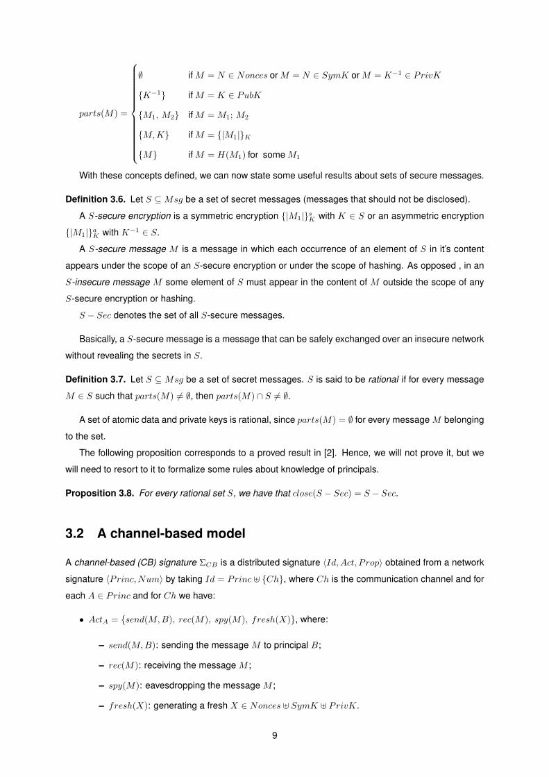
Let (i, s) and (j, z) be compatible states.

(j, z) < (j, y) ./ ... ./ (m,x) < (m,w) ./ (l, v) < (l, u) ./ (i, t) ≤ (i, s)

CLOSED(¬COMP)

Figure 4.19: New rule for synchronization.

1We can also say that ιi is compatible with ιj .

26

(j, z) (j, y)

j · · · −→ • −→ • −→ 99K · · ·

./...

./ (m,w)

m · · · 99K 99K −→ • −→ • −→ 99K 99K 99K 99K · · ·

(m,x) ./ (l, u)

l · · · 99K 99K 99K 99K −→ • −→ • −→ 99K 99K · · ·

(l, v) ./

i · · · 99K 99K 99K 99K 99K 99K −→ • −→ • −→ · · ·

(i, t) (i, s)

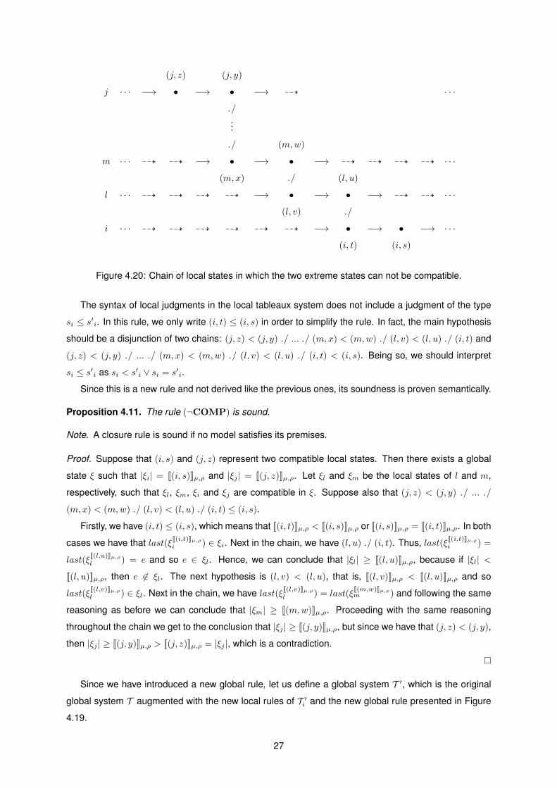
Figure 4.20: Chain of local states in which the two extreme states can not be compatible.

The syntax of local judgments in the local tableaux system does not include a judgment of the type

si ≤ s′i. In this rule, we only write (i, t) ≤ (i, s) in order to simplify the rule. In fact, the main hypothesis

should be a disjunction of two chains: (j, z) < (j, y) ./ ... ./ (m,x) < (m,w) ./ (l, v) < (l, u) ./ (i, t) and

(j, z) < (j, y) ./ ... ./ (m,x) < (m,w) ./ (l, v) < (l, u) ./ (i, t) < (i, s). Being so, we should interpret

si ≤ s′i as si < s′i ∨ si = s′i.

Since this is a new rule and not derived like the previous ones, its soundness is proven semantically.

Proposition 4.11. The rule (¬COMP) is sound.

Note. A closure rule is sound if no model satisfies its premises.

Proof. Suppose that (i, s) and (j, z) represent two compatible local states. Then there exists a global

state ξ such that |ξi| = [[(i, s)]]µ,ρ and |ξj | = [[(j, z)]]µ,ρ. Let ξl and ξm be the local states of l and m,

respectively, such that ξl, ξm, ξi and ξj are compatible in ξ. Suppose also that (j, z) < (j, y) ./ ... ./

(m,x) < (m,w) ./ (l, v) < (l, u) ./ (i, t) ≤ (i, s).

Firstly, we have (i, t) ≤ (i, s), which means that [[(i, t)]]µ,ρ < [[(i, s)]]µ,ρ or [[(i, s)]]µ,ρ = [[(i, t)]]µ,ρ. In both

cases we have that last(ξ[[(i,t)]]µ,ρi ) ∈ ξi. Next in the chain, we have (l, u) ./ (i, t). Thus, last(ξ[[(i,t)]]µ,ρi ) =

last(ξ[[(l,u)]]µ,ρl ) = e and so e ∈ ξl. Hence, we can conclude that |ξl| ≥ [[(l, u)]]µ,ρ, because if |ξl| <

[[(l, u)]]µ,ρ, then e 6∈ ξl. The next hypothesis is (l, v) < (l, u), that is, [[(l, v)]]µ,ρ < [[(l, u)]]µ,ρ and so

last(ξ[[(l,v)]]µ,ρl ) ∈ ξl. Next in the chain, we have last(ξ[[(l,v)]]µ,ρl ) = last(ξ

[[(m,w)]]µ,ρm ) and following the same

reasoning as before we can conclude that |ξm| ≥ [[(m,w)]]µ,ρ. Proceeding with the same reasoning

throughout the chain we get to the conclusion that |ξj | ≥ [[(j, y)]]µ,ρ, but since we have that (j, z) < (j, y),

then |ξj | ≥ [[(j, y)]]µ,ρ > [[(j, z)]]µ,ρ = |ξj |, which is a contradiction.

Since we have introduced a new global rule, let us define a global system T ′, which is the original

global system T augmented with the new local rules of T ′i and the new global rule presented in Figure

4.19.

27

Proposition 4.12. T ′ is sound.

Proof. The soundness of T ′ is consequence of Propositions 4.5, 4.6, 4.7 and 4.11.

The following proposition is similar to Corollary 4.8, but now for the global implication formula.

Proposition 4.13. Given Γ ∪ {@i[ϕ] ⇒ @j [ψ]} ⊆ LDTL, Γ |=DTL @i[ϕ] ⇒ @j [ψ] if there exists a

exhausted, closed T ′-tableau for {(k, 0) : Goα|@k[α] ∈ Γ} ∪ {(i, s) : ϕ} ∪ {(j, z) : ¬ψ}, where (i, s) and

(j, z) are compatible.

Proof. Let Θ be the set of local judgments {(k, 0) : Goα|@k[α] ∈ Γ} ∪ {(i, s) : ϕ} ∪ {(j, z) : ¬ψ}. If there

exists a T ′-tableau for Θ that is closed, an inductive argument applied to the soundness of T ’ guarantees

that Γ |=DTL @i[ϕ]⇒ @j [ψ].

In order to have a proposition equivalent to Corollary 4.8, we would have to prove the completeness

of T ′. But since the completeness is not fundamental to prove any of the results presented in the next

chapters, we abstained from proving it. The soundness is enough to guarantee that the proofs of the

results are correct and that is our main objective.

4.3 Rules for CB models

Regarding the axiomatization of the CB signature, note that axiom (K) can not be formulated like the

remaining axioms, that is, there is no global formula that incorporates the information given by (K).

Hence, we can not even include this axiom in the initial judgments and so there is the need to introduce

a rule that fulfills our needs in terms of applying this axiom to the tableaux for the proofs of some results

concerning CB models. For instance, we need to guarantee that given a closed set S, if a principal does

not know any message not in S, then he will not gain any information about these types of messages if

he generates, sends, receives or spies a message in S. Rule (RK) presented in Figure 4.21 translates

precisely this reasoning. Note that we should not have the universal quantifier in the premise of the rule,

since the language of the tableaux system does not allow universal quantifiers. Note that in this case,

the quantifier translates an infinite set of premises. But since we need it to guarantee the soundness of

the rule, we will undervalue this detail.

Let M ′′′ ∈Msg, M ′′ ∈ S and M ′ /∈ S.

(i, v) : ¬knows(M) ∀M /∈ S(i, v + 1) : send(M ′′′, X), X ∈ Princ | (i, v + 1) : act(M ′′), act ∈ {fresh, rec, spy}

(i, v + 1) : knows(M ′)

CLOSED(RK)

Figure 4.21: Knowledge rule for CB models.

Axiom (F2) is the only axiom with a global implication, which also means that we can not include it

in the initial judgments, once more because there is no way to express it with the syntax of the tableaux

28

system. Hence, there is the need to transform it into the closure rule (RF2) in Figure 4.22. As in rule

(¬COMP), to apply this rule in a tableau we should establish apriori the stated compatibility assump-

tion.

Rules (FRESH1) and (FRESH2), also presented in Figure 4.22, guarantee that if a fresh data item

is generated, it is generated only once. This guarantee is easily assumed when we are proving a result

semantically for a CB model, since it is the immediate consequence of the freshness axioms (F1) and

(F2). When proving such result by the tableaux system, even this simple guarantee has to be formalized

into a rule. In this particular case, we decided to introduce two rules: the first is local and guarantees that

a certain principal can not generate the same data twice; the second one is global and guarantees that

two different principals can not generate the same data, regardless of the relation between the states

where the fresh action holds.

Let (i, u) and (j, v) be compatible states, X ′ ∈ cont(M) and k 6= l.

(i, u) : fresh(X ′)(j, v) : knows(M)

CLOSED(RF2)

(i, w) : fresh(X)(i, z) : fresh(X)

(i, w) < (i, z) | (i, z) < (i, w)

CLOSED(FRESH1)

(k,w) : fresh(X)(l, z) : fresh(X)

CLOSED(FRESH2)

Figure 4.22: Freshness and uniqueness rules for CB models.

Once again, these new rules are only sound when applied to judgments that that are satisfied by CB

models, since they are the consequence of the axiomatization of the CB signature. In Chapter 5, since

we will only deal with CB models, or their augmented versions that also include the knowledge axiom

and the freshness axioms, we will apply these rules in our tableaux without referring the fact that they

should only be used when proving results for these models.

Proposition 4.14. The rules in Figures 4.21 and 4.22 are sound for CB models.

Proof. (RK): Let S be a closed set, that is, S = close(S). Let M ′′′ ∈ Msg, M ′′ ∈ S and M ′ /∈ S. Let µ

be an arbitrary CB model and ρ an assignment. Assume now that (†)µ, ρ (i, v) : ¬knows(M) ∀M /∈ S,

µ, ρ (i, v + 1) : send(M ′′′, X), for some X ∈ Princ, or µ, ρ (i, v + 1) : act(M ′′), and µ, ρ

(i, v + 1) : knows(M ′). Let [[(i, v)]]µ,ρ = k. Then, respectively, µi, ξki i ¬knows(M) ∀M /∈ S, µi, ξk+1i i

send(M ′′′, X) or µi, ξk+1i i act(M ′′), and µi, ξk+1

i i knows(M ′). By this last statement and axiom (K),

we conclude that M ′ ∈ close({M∗ |µi, ξk+1i i (Yknows(M∗)∨ rec(M∗)∨ spy(M∗)∨ fresh(M∗))}). Let

us now investigate this set.

Regardless of what is the action that holds in state (i, v + 1), we can always have that µi, ξk+1i i

Yknows(M∗), which is equivalent to µi, ξki i knows(M

∗). By (†), we conclude that M∗ ∈ S. Let us

first suppose that µi, ξk+1i i send(M ′′′, X). In this case, µi, ξk+1

i 6 i (rec(M∗)∨ spy(M∗)∨ fresh(M∗)),

29

since the semantics of DTL guarantees that there can not be two different actions in the same local

action. Hence, the gain of knowledge can only come from the previous knowledge, that is, µi, ξk+1i i

Yknows(M∗), and so we have that M∗ ∈ S. Let us now suppose that act ≡ rec, that is, µi, ξk+1i i

rec(M ′′). Then, µi, ξk+1i 6 i (spy(M∗) ∨ fresh(M∗)), again by uniqueness of actions in a local state,

and so µi, ξk+1i i (Yknows(M∗) ∨ rec(M∗)). If µi, ξk+1

i i Yknows(M∗), we conclude once more

that M∗ ∈ S. If µi, ξk+1i i rec(M∗), then it must be the case that M ′′ = M∗ and so M∗ ∈ S. The

same reasoning can be applied in the cases where act ≡ spy and act ≡ fresh and we conclude that,

regardless of the action, M∗ ∈ S.

Since S is a closed set, we can finally conclude that M ′ ∈ S, which is a contradiction to the initial

hypothesis.

(RF2): Let us suppose that (i, u) and (j, v) represent two compatible local states. Then there exists

a global state ξ such that |ξi| = [[(i, u)]]µ,ρ and |ξj | = [[(j, v)]]µ,ρ. Let µ be an arbitrary CB model and

ρ an assignment. Assume now that µ, ρ (i, u) : fresh(X) and µ, ρ (j, v) : knows(M), with X ∈

cont(M). Then µi, ξ[[(i,u)]]µ,ρi i fresh(X) and µj , ξ

[[(j,v)]]µ,ρj j knows(M), or also µi, ξi i fresh(X)

and µj , ξj j knows(M). By axiom (F2), we have µ, ξ @i[fresh(X)] ⇒∧

j∈Princ\{i}@j [¬knows(M)],

X ∈ cont(M). Then, by definition of global satisfaction relation at a global state, µ, ξ 6 @i[fresh(X)]

or µ, ξ ∧

j∈Princ\{i}@j [¬knows(M)]. By the same definition, this also means that µi, ξi 6 i fresh(X) or

µj , ξj j ¬knows(M), for every j ∈ Princ \ {i}, which is a contradiction to the assumption above and

thus the rule is sound.

(FRESH1): Since this closure rule is derived from the rules in T ′i , we will prove its soundness by

constructing a tableau, which is depicted in Figure 4.23.

(FRESH2): Let µ be an arbitrary CB model and ρ an assignment. Assume now that µ, ρ (i, w) :

fresh(X) and µ, ρ (j, z) : fresh(X), with X ∈ cont(M). Then µi, ξ[[(i,w)]]µ,ρi i fresh(X) and

µj , (ξ′j)

[[(j,z)]]µ,ρ j fresh(X), or also µi, ξi i fresh(X) and µj , ξ′j j fresh(X). Let ξ∗ be the smallest

global state that contains both ξ and ξ′, that is, ξ∗ = last(ξ ∪ ξ′) ↓. Thus µi, ξ∗i i Pfresh(X) and

µj , ξ∗j j Pfresh(X), which means there exists n and m such that n < |ξ∗i |, m < |ξ∗j | and µi, (ξ

∗i )n i

fresh(X) and µj , (ξ∗j )m j fresh(X). By property (K7), we can conclude that µi, (ξ∗i )n i knows(X)

and µj , (ξ∗j )m j knows(X). But, by axiom (F2), since i 6= j, we have that µj , (ξ∗j )m j ¬knows(M), for

any message M such that X ∈ cont(M). In particular, µj , (ξ∗j )m j ¬knows(X), which is a contradiction.

We could extend the tableaux system T ′ to include the new rules in Figures 4.21 and 4.22. We will

not do so because they are only sound for CB models and the tableaux system ought to be defined to

apply in any DTL model. But since these new rules are sound, a proposition equivalent to Proposition

4.13 for the augmented version of T ′ would be stated and proved the exact same way.

We will present other rules and their soundness will always be proved. Thus, each time a new rule

is presented, we can easily state and prove a result equivalent to Proposition 4.13 for the “extended”

version of T ′. But since the proposition would be stated and proved the exact same way, we abstain from

doing so for the sake of clarity. Thus, each time we proof a certain result, which requires the “extended”

version of T ′, and we affirm resorting to Proposition 4.13, we are actually considering this proposition

30

(i,w):fresh(X)

(i,z):fresh(X)

(i,0):Go(fresh(X)⇒knows(X))

(i,0):Go(knows(X)⇒Go(knows(X)))

(i,0):Go(fresh(N)⇒Y¬knows(m)), N∈cont(m)

Go ⇒(i,w):knows(X)

Go ⇒(i,z):knows(X)

Go ⇒(i,w):Go(knows(X))

Go ⇒(i,z):Go(knows(X))

Go

(i,w):knows(X)

(i,w):G(knows(X))

Go

(i,w):knows(X)

(i,w):G(knows(X))

(i,w)<(i,z) (i,z)<(i,w)

Go ⇒ Go ⇒(i,z):Y¬knows(X) (i,w):Y¬knows(X)

Y Y(i,z−1):¬knows(X) (i,w−1):¬knows(X)

DIF DIF(i,w)<(i,z−1) (i,z−1)<(i,w)

G DTRANS(i,z−1):knows(X) (i,z−1)<(i,z−1)

ABS NLOOPCLOSED CLOSED

(i,z)<(i,w−1) (i,w−1)<(i,z)

G DTRANS(i,w−1):knows(X) (i,w−1)<(i,w−1)


Figure 4.23: Tableau for proving the soundness of rule (FRESH1).

for the “extended” version of T ′.

31

32

Chapter 5

Authentication property for NSL

protocol

In this chapter, we will show that the authentication property authResp,Init,3B,A (A,B,N1, N2) for an honest

agent B holds for the NSL protocol.

5.1 Rules for modeling NSL protocol

In order to prove the three main results of this chapter using the tableaux system, there is the need to

establish some rules concerning the modeling of the NSL protocol. As mentioned in Chapter 3, in a

NSL protocol, while an intruder can act freely, an honest agent does not do so. We require that honest

agents do not play two different roles in the same run and that they strictly follow the protocol. These

impositions have rules in Figures 5.1, 5.2 and 5.3 as a consequence. The rules in Figures 5.1 and

5.2 are straightforward, since they are the immediate translation of the each role instantiation. The rule

(RH1) simply guarantees that no honest agent freshly generates the same data in two different runs.

Let i ∈ Hon.

(i, v) : send({|N2|}aKr , r)(i, v) : P(rec({|N1;N2; r|}aKi) ∧ P(send({|N1; i|}aKr , r) ∧ Pfresh(N1)))

(RNSLI1)

(i, v) : rec({|N1;N2; r|}aKi(i, v) : P(send({|N1; i|}aKr , r) ∧ Pfresh(N1))

(RNSLI2)

(i, v) : send({|N1; i|}aKr , r)(i, v) : Pfresh(N1)

(RNSLI3)

Figure 5.1: Rules for modeling the role of the initiator in a NSL protocol.

33

Let r ∈ Hon.

(r, v) : rec({|N2|}aKr )(r, v) : P(send({|N1;N2; r|}aKi , i) ∧ P(fresh(N2) ∧ Prec({|N1; i|}aKr )))

(RNSLR1)

(r, v) : send({|N1;N2; r|}aKi , i)(r, v) : P(fresh(N2) ∧ Prec({|N1; i|}aKr ))

(RNSLR2)

(r, v) : fresh(N2)

(r, v) : Prec({|N1; i|}aKr )(RNSLR3)

Figure 5.2: Rules for modeling the role of the responder in a NSL protocol.

Let i ∈ Hon, N ∈ Nonces and Run1, Run2 be two different runs.

(i, v) : fresh(N)Run1

(i, v) : fresh(N)Run2

CLOSED(RH1)

Figure 5.3: Rule for modeling fresh actions executed by honest agents in a NSL protocol.

Proposition 5.1. The rules in Figures 5.1, 5.2 and 5.3 are sound for NSL models.

Proof. In the NSL protocol, honest principals strictly follow the protocol. Hence, the rules in Figures 5.1

and 5.2 are sound for NSL models because they are the exact translation of each role instantiation in

a NSL protocol. Concerning the rule (RH1), it states that no honest agent can generate the same data

to participate in two different runs, which is one of the characteristics of the NSL protocol, described in

subsection 3.3.1.

This chapter is only dedicated to the NSL protocol and so we will apply these rules in the tableaux

built to prove the results of this chapter without referring the fact that they are only sound when used to

prove results for NSL models.

5.2 Derived rules to simplify the tableaux

Once again, we introduce some rules that allow us to simplify our tableaux, making them smaller and

especially less repetitive. The two rules in Figure 5.4 translate arguments that were used in all of the

constructed tableaux for the proofs of the lemmas in this chapter. So, by introducing these rules, we can

simply apply them instead of repeating the same arguments in the tableaux.

Since the rules in Figure 5.4 are derived from the rules in T ′, we can prove their soundness by

constructing a tableau for each rule.

Proposition 5.2. The derived rules (RS1) and (RS2) are sound.

Proof. (RS1): The corresponding tableau for the soundness of this rule is depicted in Figure 5.5. Let

(i, v′i) and (Ch, v′Ch) be compatible (in a global state) and (i, v′i+1) and (Ch, v′Ch+1) also be compatible

34

Let (i, v′i) and (Ch, v′Ch) be compatible, (i, v′i + 1) and (Ch, v′Ch + 1) also be compatible, j ∈ Princ,m ∈Msg and acti ∈ {send(m, j), rec(m), spy(m)}.

(i, v′i + 1) : acti(Ch, 0) : Go(acti �Ch actCh)

(Ch, v′Ch + 1) : actCh(RS1)

Let M ′ ∈Msg.

(Ch, v′Ch) :∧

C,D∈Princ¬Poin(C,M ′, D)

(Ch, v′Ch + 1) :∨

C,D∈PrincPoin(C,M ′, D)

(Ch, v′Ch + 1) : in(Y,M ′,W ), Y,W ∈ Princ(RS2)

Figure 5.4: Derived rules to simplify the tableaux.

(in another global state). Note that these compatibility assumptions allow us to apply rule (¬COMP) to

close some branches of the tableau.

(i,v′i+1):acti,

(Ch,0):Go(acti�ChactCh))

Go ⇒(i,v′i+1): c©Ch(actCh)

c©(Ch,v′′ch):actCh

(i,v′i+1)./(Ch,v′′ch)

SYM(Ch,v′′ch)./(i,v

′i+1)

SUCC(i,v′i)<(i,v′i+1)

TR(Ch,v′′ch)<(Ch,v′Ch+1) (Ch,v′′ch)=(Ch,v′Ch+1) (Ch,v′Ch+1)<(Ch,v′′ch)

TR CONG ¬COMP(Ch,v′′ch)<(Ch,v′Ch) (Ch,v′′ch)=(Ch,v′Ch) (Ch,v′Ch)<(Ch,v′′ch)

¬COMP CONG DTRANSCLOSED (i,v′i+1)./(Ch,v′ch) (Ch,v′Ch)<(Ch,v′Ch)

¬COMP NLOOPCLOSED CLOSED

(Ch,v′Ch+1):actCh CLOSED

Figure 5.5: Tableau for the soundness of rule (RS1).

(RS2): The corresponding tableau for the soundness of this rule is depicted in Figure 5.6.

When applying the rule (∨

), the tableau should be divided in as many branches as the number of

principals involved in the protocol. Since we use this rule twice, the tableau should be, in fact, divided in

as many combinations involving two principals as possible. As mentioned in Chapter 4, where this same

rule was presented, we do not know how many principals are involved in a protocol and so we divide

the tableau in as many branches as necessary in order to represent all principals (or all combinations).

This reasoning will be done several times in the tableaux that follow and so we will not justify it in the

future. In this specific case, since it does not matter with what principals we are dealing, Y and W are

considered to be any principals, which is one important detail in the conclusion of this rule.

35

(Ch,v′Ch):∧

C,D∈Princ¬Poin(C,M

′,D)

(Ch,v′Ch+1):∨

C,D∈PrincPoin(C,M

′,D)∨(Ch,v′Ch+1):

∨D∈Princ

Poin(Y,M′,D)∨

(Ch,v′Ch+1):Poin(Y,M′,W )

Po

(Ch,v′Ch+1):in(Y,M ′,W ) (Ch,v′Ch+1):Pin(Y,M ′,W )

P(Ch,v∗Ch)<(Ch,v′Ch+1)

(Ch,v∗Ch):in(Y,M′,W )∧

(Ch,v′Ch):∧

D∈Princ¬Poin(Y,M

′,D)∧(Ch,v′Ch):¬Poin(Y,M

′,W )

¬Po

(Ch,v′Ch):¬in(Y,M′,W )

(Ch,v′Ch):¬Pin(Y,M′,W )

DIF(Ch,v∗Ch)<(Ch,v′Ch) (Ch,v′Ch)<(Ch,v∗Ch)

¬P DTRANS(Ch,v∗Ch):¬in(Y,M

′,W ) (Ch,v′Ch)<(Ch,v′Ch)


Figure 5.6: Tableau for the soundness of rule (RS2).

5.3 Auxiliary lemmas

Before showing the main proposition that guaranties that NSL protocol authenticates the initiator, we

have to prove two lemmas stated in [2].

The first states that if A and B are honest and A does not send the required message {|N2|}aKB to

B, then no other agent could ever do it either.

Lemma 5.3. Let:

• A,B ∈ Hon;

• µ a NSL model;

• ξ be a global state such that µ, ξ @B [fresh(N2) ∧ Fsend({|N1;N2;B|}aKA , A)];

• IMN2be the set of messages {N2,K

−1A }-insecure or that contain N2 outside a sub-message

{|N1;N2;B|}aKA .

For every global state ξ′ ⊇ ξ, if

µ, ξ′ 6 @A[Posend({|N2|}aKB , B)]

then, for every E ∈ Princ with E /∈ {A,B} and every message M ∈ IMN2the following holds:

µ, ξ′ @Ch[∧

C,D∈Princ¬Poin(C,M,D)] and µ, ξ′ 6 @E [knows(M)].

36

Proof. In the tableaux built for this proof, as well as for the proofs of the following results, we will use

boxes to avoid repeating sub-tableaux in the figures.

Also for the sake of repeating the construction of very similar tableaux, the ones that prove this

lemma can also be used to prove Lemma 5.5. This implies that some of their content are, in a certain

way, abstract. For this matter, we should consult Table 5.1 and substitute the generalized judgments and

sub-tableaux for the ones of the corresponding lemma. Specifically, for this lemma we should substitute

N∗ by N2, HN∗ by HN2 and TBN∗ by TBN2 whenever they appear.

To prove this lemma, we will resort to Proposition 2.13 (Global Invariance Rule) and being so, let us

start the proof by the base case.

Base: ξ = ξ′

To proof the base case, we will suppose, by contradiction, that either µ, ξ @Ch[∨

C,D∈PrincPoin(C,M,

D)] or µ, ξ @E [knows(M)], where M is a certain message that belongs to IMN2 . The tableau made

for this proof is then closed and is depicted in Figure A.1.

But before considering the tableau itself, we have to establish that (A, vA), (B, vB), (E, vE), (P, vP )

and (Ch, vCh) are compatible in the global state ξ, where P is any principal such that P /∈ {A,B,E}. As

usual, in order to use the rule (¬COMP), these compatibility assumptions are crucial.

With these conditions established, let us now make some observations regarding the not so obvious

steps in the tableau.

Note that the hypothesis (A, vA) : ¬Posend({|N2|}aKB , B) was not taken into account because it was

not necessary to the development of the tableau. This will also be true in many cases of the induction

step. For this lemma, the sub-tableau that follows TB1 is TB1N2 , depicted in Figure A.2. In this tableau,

X and Y are considered to be any principals, consequence of applying twice the rule (∨

), as explained

in the previous section.

The sub-tableau that follows is TB1.1, depicted in Figure A.4. In this tableau, the division into cases

1. and 2. is such that for the first one we substitute X for B (and that is why this branch continues with

local states of the form (B, vB) and not (X, vx)) and for the second one we can substitute X either any

principal of the set SP , which for this lemma is {A,E, P} (and that is why the local states of the form

(X, vx) are not substituted).

Note that since we are assuming that M ∈ IMN2, M is such that N2 ∈ cont(M). In the first and

second branches of case 1., we have that (B, vB − 1) does not know M because M contains N2 and

N2 was only generated in (B, vB − 1).

A similar deduction was made to close the second branch in the main tableau TB1 (the case where

we suppose that (E, vE) knows M ) and to close the first and second branches of case 2.. The only

difference in this cases is that we were not dealing with principal B, which is the one that executed

fresh(N2). Then, and since we established that (A, vA), (B, vB), (E, vE), and(P, vP ) are compatible,

we can apply the rule (RF2) to conclude that each state (X, vX), X ∈ {A,E, P}, can not know any

message that contains N2, and so can not know M .

Induction step: Let us assume that the properties hold for a global state ξ′ ⊇ ξ and consider every

37

possible superstate ξ′′ = ξ′ ∪ {e}.

From axiom (P5) we conclude that e can not be an event shared by two principals. At most, it can be

shared with the channel. Therefore, we consider three distinct cases:

(i): e ∈ EvA(ii): e ∈ EvB(iii): e ∈ EvELike in the base case, the proofs will be done by contradiction, that is, we will suppose that ei-

ther µ, ξ′′ @Ch[∨

C,D∈PrincPoin(C,M ′, D)] or µ, ξ′′ @E [knows(M ′)], where M ′ is a certain mes-

sage belonging to IMN2, and the tableaux that correspond them are, naturally, closed. Since we sup-

pose that (†)µ, ξ′ 6 @Ch[∧

C,D∈PrincPoin(C,M,D)] and (‡)µ, ξ′ 6 @E [knows(M)], for every message

M ∈ IMN2 , then we also can establish without a doubt that µ, ξ′ 6 @Ch[∧

C,D∈PrincPoin(C,M ′, D)] and

µ, ξ′ 6 @E [knows(M ′)]. This way, we do not have any universal quantifier in the judgments of the

tableaux, which is consistent with the language allowed in the tableaux system.

The tableaux built to proof the different hypothesis of cases (i) and (ii) and so some of their content

are, in a certain way, abstract. Specifically, to prove the different scenarios of case (i), we should

substitute I by A, whereas for case (ii), we substitute I by B.

For cases (i) and (ii), note that ξ′E = ξ′′E , since e /∈ EvE .

• Case (i)

1. αA(e) = fresh(N)

For this case, the corresponding tableau for the proof is tableau T1 depicted in Figure 5.7.

Apriori to the tableau, we have to establish the following compatibility assumptions, like we

did for the base case:

– (A, v′A), (E, v′E) and (Ch, v′Ch) are compatible in the global state ξ′;

– (A, v′A + 1), (E, v′E) and (Ch, v′Ch) are compatible in the global state ξ′′.

T1(Ch,v′Ch):

∧C,D∈Princ

¬Poin(C,M′,D)

(E,v′E):¬knows(M ′)

(I,v′I+1):fresh(N)

(Ch,v′Ch):∨

C,D∈PrincPoin(C,M

′,D) (E,v′E):knows(M ′)

ABS ABSCLOSED CLOSED

Figure 5.7: Tableau T1 for the proof of cases (i)-1 and (ii)-1 of Lemmas 5.3 and 5.5.

In this case, the action associated with the event is a fresh action and so, by axiom (P6), it

can not be shared with the channel. This is why the local state (Ch, v′Ch) was considered to

be also compatible with (A, v′A + 1) in ξ′′, whereas in the following actions, which are shared

with the channel, the local state (Ch, v′Ch + 1) is the one compatible with (A, v′A + 1) in ξ′′.

And since we assume that (Ch, v′Ch) :∨

C,D∈PrincPoin(C,M ′, D), we can immediately close

the corresponding branch, since it contradicts the initial hypothesis.

38

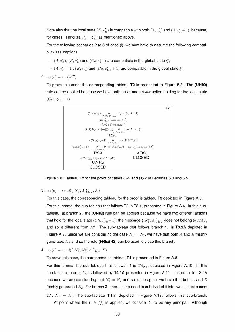
Note also that the local state (E, v′E) is compatible with both (A, v′A) and (A, v′A+1), because,

for cases (i) and (ii), ξ′E = ξ′′E , as mentioned above.

For the following scenarios 2 to 5 of case (i), we now have to assume the following compati-

bility assumptions:

– (A, v′A), (E, v′E) and (Ch, v′Ch) are compatible in the global state ξ′;

– (A, v′A + 1), (E, v′E) and (Ch, v′Ch + 1) are compatible in the global state ξ′′.

2. αA(e) = rec(M ′′)

To prove this case, the corresponding tableau T2 is presented in Figure 5.8. The (UNIQ)

rule can be applied because we have both an in and an out action holding for the local state

(Ch, v′Ch + 1).

T2(Ch,v′Ch):

∧C,D∈Princ

¬Poin(C,M′,D)


(I,v′I+1):rec(M ′′)

(I,0):Go(rec(m)�Ch

∨P∈Princ

out(P,m,I))

RS1(Ch,v′Ch+1):

∨P∈Princ

out(P,M ′′,I)

(Ch,v′Ch+1):∨

C,D∈PrincPoin(C,M


RS2 ABS(Ch,v′Ch+1):in(Y,M ′,W ) CLOSED

UNIQCLOSED

Figure 5.8: Tableau T2 for the proof of cases (i)-2 and (ii)-2 of Lemmas 5.3 and 5.5.

3. αA(e) = send({|N◦1 ;A|}aKX , X)

For this case, the corresponding tableau for the proof is tableau T3 depicted in Figure A.5.

For this lemma, the sub-tableau that follows T3 is T3.1, presented in Figure A.6. In this sub-

tableau, at branch 2., the (UNIQ) rule can be applied because we have two different actions

that hold for the local state (Ch, v′Ch+1): the message {|N◦1 ;A|}aKX does not belong to IMN2

and so is different from M ′. The sub-tableau that follows branch 1. is T3.2A depicted in

Figure A.7. Since we are considering the case N◦1 = N2, we have that both A and B freshly

generated N2 and so the rule (FRESH2) can be used to close this branch.

4. αA(e) = send({|N◦1 ;N◦2 ;A|}aKX , X)

To prove this case, the corresponding tableau T4 is presented in Figure A.8.

For this lemma, the sub-tableau that follows T4 is T4N2 , depicted in Figure A.10. In this

sub-tableau, branch 1., is followed by T4.1A presented in Figure A.11. It is equal to T3.2A

because we are considering that N◦2 = N2 and so, once again, we have that both A and B

freshly generated N2. For branch 2., there is the need to subdivided it into two distinct cases:

2.1. N◦1 = N2: the sub-tableau T4.3, depicted in Figure A.13, follows this sub-branch.

At point where the rule (∨

) is applied, we consider Y to be any principal. Although

39

{|N2;X|}aKA is {N2,K−1A }-secure, it contains N2 outside a sub-message {|N1;N2;B|}aKA

and so belongs to IMN2 . This is why we can use the hypothesis (†) to assume in the be-

ginning of the tableau that (Ch, v′Ch) :∧

C,D∈Princ¬Poin(C, {|N∗;X|}aKI , D)1 (for this case,

N∗ = N2 and I = A), which is fundamental to close this sub-tableau.

2.2. N◦1 6= N2: the message {|N◦1 ;N◦2 ;A|}aKX does not belong to IMN2and so it is different

fromM ′. Hence, the (UNIQ) rule can be applied because we have two different in actions

that hold for the local state (Ch, v′Ch + 1).

5. αA(e) = send({|N◦2 |}aKX , X)

For this case, the corresponding tableau for the proof is tableau T5 presented in Figure A.14.

In this case, we need to consider the judgment in brackets. It has to be ignored to prove case

(ii) and Lemma 5.5.

The sub-tableau that follows the main one is T5.1 depicted in Figure A.15. In this tableau,

branch 1. follows a similar reasoning as in T4.3. The main difference now is that we do not

know if the message {|N◦1 ;N2;X|}aKA belongs to IMN2. We can observe immediately that

it is {N2,K−1A }-secure but we need to consider two distinct cases to come to a conclusion.

They are presented in tableau T5.2A, presented in Figure A.16:

1. N◦1 6= N1 or X 6= B : the message {|N◦1 ;N2;X|}aKA contains N2 outside the sub-message

{|N1;N2;B|}aKA and so it belongs to IMN2. Therefore, we can use hypothesis (†) to ini-

tially acknowledge that (Ch, v′Ch) :∧

C,D∈Princ¬Poin(C, {|N◦1 ;N∗;X|}aKI , D) (for this case,

N∗ = N2 and I = A), which leads to a contradiction and to the consequence closure of

the tableau T5.2B, depicted in Figure A.16.

2. N◦1 = N1 and X = B: since we are in the case where N◦2 = N2 and now we have also

that X = B, send({|N2|}aKB , B) holds for (A, v′A + 1), which is a contradiction to the initial

assumption in brackets.

Also in tableau T5.1, at branch 2. where we consider N◦2 6= N2, the (UNIQ) rule can be

applied as in the previous tableaux because we have two different in actions that hold for the

local state (Ch, v′Ch + 1): {|N◦2 |}aKX 6∈ IMN2 and so is different from M ′.

• Case (ii)

1. αB(e) = fresh(N)

For this case, the proof is the same as for the case (i) - 1 and so the corresponding tableau is

also depicted in Figure 5.7.

The equivalent compatibility assumptions that we now need to establish apriori are the fol-

lowing:

– (B, v′B), (E, v′E) and (Ch, v′Ch) are compatible in the global state ξ′;

– (B, v′B + 1), (E, v′E) and (Ch, v′Ch) are compatible in the global state ξ′′.

1Once again, we do this type of reasoning in order to avoid universal quantifiers in the judgments of the tableaux.

40

For the following scenarios 2 to 5 of case (ii), we need to establish the same compatibility

assumptions as in case (i), but now for principal B:

– (B, v′B), (E, v′E) and (Ch, v′Ch) are compatible in the global state ξ′;

– (B, v′B + 1), (E, v′E) and (Ch, v′Ch + 1) are compatible in the global state ξ′′.

2. αB(e) = rec(M ′)

Likewise, the proof is the same as for the case (i) - 2 and so the corresponding tableau is

presented in Figure 5.8.

3. αB(e) = send({|N◦1 ;B|}aKX , X)

Likewise, the proof is similar to the case (i) - 3 and so the corresponding tableau is also

depicted in Figure A.5. Since we are still proving Lemma 5.5, the sub-tableau that follows T3

is T3.1 (see Figure A.6). But now, for this case, the sub-tableau that follows T3.1 is T3.2BN2 ,

presented in Figure A.7.

In this sub-tableau, the second branch of the trichotomy is closed because B executed

fresh(N2) both in an initiator run and a responder run. Since B is an honest principal and

we are considering a NSL model, we can use the rule (RH1) to close this branch. The other

branches can be closed by rule (FRESH1) because (B, vB) and (B, v∗B) are distinct local

states of agent B that both freshly generate N2.

4. αB(e) = send({|N◦1 ;N◦2 ;B|}aKX , X)

Like in the previous cases, the proof is similar to the case (i)-4 and so the corresponding

tableau is also depicted in Figure A.8. The sub-tableau that follows T4 is, as expected, T4N2

(see Figure A.10) and the sub-tableau that follows its branch 1. is, for this case, T4.1BN2

presented in Figure A.12.

In this sub-tableau, the first and last branches of the trichotomy are closed for the same

reason as in T3.2B. In the middle branch, we split it into two possible scenarios:

1. X = A and N◦1 = N1: in this case, the message {|N1;N2;A|}aKA does not belong to IMN2

and so it can not be M ′, thus two different in actions hold for the local state (Ch, v′Ch + 1).

2. X 6= A or N◦1 6= N1: in this case, B freshly generates N2 in two different runs, in which he

plays the responder role at both, but in one he first receives {|N1;A|}aKB , while in the other

he first receives {|N◦1 ;X|}aKB .

The sub-tableau that follows the sub-branch 2.1. in T4N2is also T4.3 (see Figure A.13). In this

case, we can immediately conclude that {|N2;X|}aKB ∈ IMN2 because it is not {N2,K−1A }-

secure and thus the initial judgment (Ch, v′Ch) :∧

C,D∈Princ¬Poin(C, {|N∗;X|}aKI , D) is also

correct for this case, where N∗ = N2 and I = B.

5. αB(e) = send({|N◦2 |}aKX , X)

Likewise, the proof is similar to the case (i) - 5 and so the corresponding tableau is also

presented in Figure A.14, but now ignoring the judgment written in brackets, since the local

state (A, v′A + 1) is not even defined in this case. The sub-tableau that follows the main one

is also T5.1 (see Figure A.15).

41

The sub-tableau that follows T5.1 is, for this case, T5.2B (see Figure A.16). In this case,

we easily conclude that the message {|N◦1 ;N2;X|}aKB is {N2,K−1

A }-insecure, thus belonging

to IMN2 . Hence, we can ignore the tableau T5.2A and conclude that the initial judgment

(Ch, v′Ch) :∧

C,D∈Princ¬Poin(C, {|N◦1 ;N∗;X|}aKI , D) is also correct for this case, where N∗ =

N2 and I = B.

• Case (iii)

Since we are assuming e ∈ EvE , the local state (E, v′E+1) is now defined and so we can not close

the branch where we suppose that E knows M ′, for M ′ ∈ IMN2, by using the same argument as in

the previous cases. Semantically, we would resort to axiom (K). Since we wish to prove this case

by using the tableaux system, we will use rule (RK) to close the mentioned branch. But for that,

we need to prove that the complement of IMN2is a closed set. Thus, let us prove the following

proposition:

Proposition 5.4. IMN2 ∩ close(Msg \ IMN2) = ∅.

Proof. Let us recall the definition of IMN2:

IMN2= {M ∈Msg |M is {N2,K

−1A }-insecure or M contains N2 outside the sub-message

{|N1;N2;B|}aKA}.

Then,

Msg \ IMN2= {M ∈Msg |M is {N2,K

−1A }-secure and M does not contain N2 outside the

sub-message {|N1;N2;B|}aKA}.

Note that:

1. Since {N2,K−1A } is a rational set, by Proposition 3.8, we can conclude that ifM ∈ close(Msg\

IMN2), then M is {N2,K

−1A }-secure;

2. {|N1;N2;B|}aKA ∈Msg \ IMN2 . Then {|N1;N2;B|}aKA ∈ close(Msg \ IMN2);

3. By 1., K−1A /∈ close(Msg \ IMN2). Thus, the message {|N1;N2;B|}aKA can not be analysed

and so, besides {|N1;N2;B|}aKA , there is no message in close(Msg\IMN2) that contains N2.

Let us now suppose that there exists a message M belonging to both IMN2and close(Msg \

IMN2). By 1., we conclude that M contains N2 outside the sub-message {|N1;N2;B|}aKA . But, by

3., that is not possible, and so IMN2 ∩ close(Msg \ IMN2) = ∅, that is, Msg \ IMN2 = close(Msg \

IMN2).

Note that, for this case, we need to consider the original assumption (‡), in order to apply the rule

(RK). This assumption should not be used in the tableaux, since it contains a universal quantifier.

But, as mentioned in Chapter 4, this quantifier is essential for the soundness of the rule, and so

we will undervalue this detail.

42

1. αE(e) = fresh(N)

For this case, the corresponding tableau for the proof is depicted in Figure 5.9. The proof

is similar to the one of case (i)-1 and so we have to establish the following compatibility

assumptions:

– (E, v′E) and (Ch, v′Ch) are compatible in the global state ξ′;

– (E, v′E + 1) and (Ch, v′Ch) are compatible in the global state ξ′′.

T6(Ch,v′Ch):

∧C,D∈Princ

¬Poin(C,M′,D)

(E,v′E):¬knows(M)

(E,v′E+1):fresh(N)

(Ch,v′Ch):∨

C,D∈PrincPoin(C,M

′,D) (E,v′E+1):knows(M ′)

ABS RKCLOSED CLOSED

Figure 5.9: Tableau T6 for the proof of case (iii)-1 of Lemmas 5.3 and 5.5.

For the rightmost branch of the tableau, the rule (RK) can be applied because we have proved

that the complement of IMN2 is a closed set and N /∈ IMN2 , since the only nonce that

belongs to IMN2is N2 itself.

For the following scenarios 2 to 4 of case (iii), we also need to establish some compatibility

assumptions, like we did for the previous cases:

– (E, v′E) and (Ch, v′Ch) are compatible in the global state ξ′;

– (E, v′E + 1) and (Ch, v′Ch + 1) are compatible in the global state ξ′′.

2. αE(e) = send(M ′′, X)

For this case, the corresponding tableau for the proof is tableau T7 presented in Figure 5.10.

At branch 2., the rule (UNIQ) is used because since we are assuming that M ′ 6= M ′′, we have

that both actions in(E,M ′′, X) and in(Y,M ′,W ), which are different, hold for the local state

(Ch, v′Ch + 1).

3. αE(e) = rec(M ′′)

To prove this case, the corresponding tableau T8 is depicted in Figure A.17.

The leftmost branch can be closed by rule (UNIQ) because we have both an in and an out

action holding (Ch, v′Ch + 1).

For branch 1., we should substitute IMN∗ by IMN2. Thus, in this branch, we are in the case

whereM ′′ ∈ IMN2and so we can also initially assume that (Ch, v′Ch) :

∧C,D∈Princ

¬Poin(C,M ′′,

D), as a consequence of (†). As usual, where we apply the rule (∨

), we consider X to be

any principal.

For branch 2., we are in the conditions of applying rule (RK).

4. αE(e) = spy(M ′′)

For this case, the corresponding tableau for the proof is tableau T9 depicted in Figure A.18.

The proof is practically the same as in 3. and so we will abstain from explaining the tableau.

43

T7(Ch,v′Ch):

∧C,D∈Princ

¬Poin(C,M′,D)


(E,v′E+1):send(M ′′,X)

(E,0):Go(send(M′′,X)⇒Y(knows(M ′′)∧knows(X)))

(E,0):Go(send(M′′,X)�Chin(E,M

′′,X))

Go ⇒(E,v′E+1):Y(knows(M ′′)∧knows(X))

Y(E,v′E):knows(M ′′)∧knows(X)

∧(E,v′E):knows(M ′′)

(E,v′E):knows(X)

RS1(Ch,v′Ch+1):in(E,M ′′,X)

(Ch,v′Ch+1):∨

C,D∈PrincPoin(C,M


RS2 RK(Ch,v′Ch+1):in(Y,M ′,W ) CLOSED

1.M′ = M′′ 2.M′ 6= M′′

(E,v′E):knows(M ′) UNIQABS CLOSED

CLOSED

Figure 5.10: Tableau T7 for the proof of case (iii)-2 of Lemmas 5.3 and 5.5.

N∗ N2 N∗1

HN∗ (B,vB):fresh(N2)∧Fsend({|N1;N2;B|}aKA ,A)(A,vA):fresh(N2)∧Fsend({|N1;N2;A|}aKZ ,Z)

(B,vB):fresh(N∗1 )∧Fsend({|N∗1 ;B|}

aKA

,A)

TBN∗

∧(B,vB):fresh(N2)

(B,vB):Fsend({|N1;N2;B|}aKA ,A)

∧(B,vB):fresh(N∗1 )

(B,vB):Fsend({|N∗1 ;B|}aKA

,A)

Table 5.1: Table with the judgments and sub-tableaux to substitute in the main tableaux of the proofs ofLemmas 5.3 and 5.5.

The next states that if an honest agent is playing the responder role in two different protocol runs,

one initiated by an honest agent and the other one by the intruder, then it will not mix the relevant data

of the two runs.

Lemma 5.5. Let:

• A,B ∈ Hon;

• µ be a NSL model;

• ζ be a global state such that µ, ζ @A[fresh(N2) ∧ Fsend({|N1;N2;A|}aKZ , Z)];

• ξ be a global state such that µ, ξ @B [fresh(N∗1 ) ∧ Fsend({|N∗1 ;B|}aKB , A)];

• IMN∗1be the set of messages {N∗1 ,K−1A ,K−1B }-insecure or that contain {|N∗1 ;N2;A|}aKB or

{|N∗1 ;X|}aKY with X 6= B or Y 6= A, or {|N ;N∗1 ;X|}aKY with any N , X, Y .

44

For every global state ξ′ ⊇ ξ, every E ∈ Princ with E /∈ {A,B} and every message M ∈ IMN∗1the

following holds:

µ, ξ′ 6 @Ch[∧

C,D∈PrincPoin(C,M,D)] and µ, ξ′ 6 @E [knows(M)].

The original lemma in [2] stated that µ, ξ′ 6 @Ch[∧

C,D∈Princin(C,M,D)]. We included the past in

the formula so that we could reason by induction and prove the result using the tableau system. If we

did not modify the formula, we would not know if for a global state between ξ and ξ′ there could be

an in action for the channel that includes a message in IMN∗1. By induction, we immediately conclude

that there can not be and so the simplest and equivalent solution is to include the past in the property.

The only question is that we are in fact stating that even for a state ξ∗ smaller than ξ we have µ, ξ∗ 6

@Ch[∧

C,D∈Princin(C,M,D)], which is redundant, in the sense that N∗1 has not yet been generated and

so no principal could ever sent a message containing N∗1 .

Proof. The proof of this lemma is very similar to the proof of the Lemma 5.3. Being so, we will also

prove this new lemma by induction, resorting Proposition 2.13, and, as mentioned above, we can use

the tableaux built to prove the previous lemma for this proof, just by consulting Table 5.1 and substituting

the generalized judgments and sub-tableaux for the ones corresponding to the this lemma. Specifically,

we should now substitute N∗ by N∗1 , HN∗ by HN∗1and TBN∗ by TBN∗1

, whenever they appear. We

will not repeat the arguments to justify the same steps in the tableaux. Instead, we will only clarify the

differences between the proofs.

Base: ξ = ξ′

Like we did for the proof of the base case of Lemma 5.3, we will suppose, by contradiction, that either

µ, ξ @Ch[∨

C,D∈PrincPoin(C,M,D)] or µ, ξ @E [knows(M)], where M is a message that belongs to

IMN∗1. The corresponding tableau is also tableau TB1 (see Figure A.1).

We also have to establish apriori the following compatibility assumption: (B, vB), (E, vE), (P, vP ) and

(Ch, vCh) are compatible in a global state ξ, where P is any principal such that P /∈ {B,E}.

For this lemma, the sub-tableau that follows TB1 is TB1N∗1, depicted in Figure A.3. The sub-tableau

that follows is also TB1.1 (see Figure A.4), but now we have that SP = {A,E, P}. The remaining

arguments that justify the steps in this last tableau are the same as in the proof of Lemma 5.3, with the

obvious difference that now M is such that N∗1 ∈ cont(M) and so the arguments should be adapted to

the nonce N∗1 , instead of N2.

Induction step: Like in the proof of the previous lemma, we will assume that the properties hold for

a global state ξ′ ⊇ ξ and consider every possible superstate ξ′′ = ξ′ ∪ {e}. Again from axiom (P5), we

conclude that e can not be an event shared by two principals. At most, it can be shared with the channel

and therefore, we consider three distinct cases:

(i): e ∈ EvA

(ii): e ∈ EvB

(iii): e ∈ EvE

45

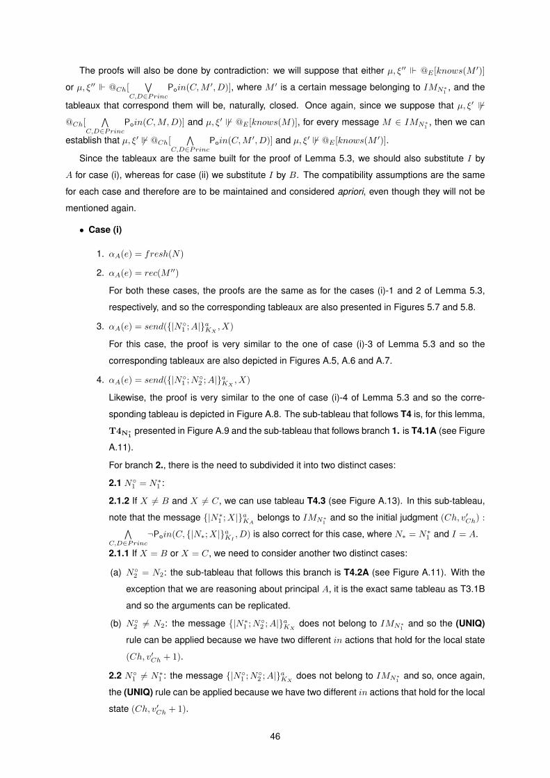
The proofs will also be done by contradiction: we will suppose that either µ, ξ′′ @E [knows(M ′)]

or µ, ξ′′ @Ch[∨

C,D∈PrincPoin(C,M ′, D)], where M ′ is a certain message belonging to IMN∗1

, and the

tableaux that correspond them will be, naturally, closed. Once again, since we suppose that µ, ξ′ 6

@Ch[∧

C,D∈PrincPoin(C,M,D)] and µ, ξ′ 6 @E [knows(M)], for every message M ∈ IMN∗1

, then we can

establish that µ, ξ′ 6 @Ch[∧

C,D∈PrincPoin(C,M ′, D)] and µ, ξ′ 6 @E [knows(M ′)].

Since the tableaux are the same built for the proof of Lemma 5.3, we should also substitute I by

A for case (i), whereas for case (ii) we substitute I by B. The compatibility assumptions are the same

for each case and therefore are to be maintained and considered apriori, even though they will not be

mentioned again.

• Case (i)

1. αA(e) = fresh(N)

2. αA(e) = rec(M ′′)

For both these cases, the proofs are the same as for the cases (i)-1 and 2 of Lemma 5.3,

respectively, and so the corresponding tableaux are also presented in Figures 5.7 and 5.8.

3. αA(e) = send({|N◦1 ;A|}aKX , X)

For this case, the proof is very similar to the one of case (i)-3 of Lemma 5.3 and so the

corresponding tableaux are also depicted in Figures A.5, A.6 and A.7.

4. αA(e) = send({|N◦1 ;N◦2 ;A|}aKX , X)

Likewise, the proof is very similar to the one of case (i)-4 of Lemma 5.3 and so the corre-

sponding tableau is depicted in Figure A.8. The sub-tableau that follows T4 is, for this lemma,

T4N∗1presented in Figure A.9 and the sub-tableau that follows branch 1. is T4.1A (see Figure

A.11).

For branch 2., there is the need to subdivided it into two distinct cases:

2.1 N◦1 = N∗1 :

2.1.2 If X 6= B and X 6= C, we can use tableau T4.3 (see Figure A.13). In this sub-tableau,

note that the message {|N∗1 ;X|}aKA belongs to IMN∗1and so the initial judgment (Ch, v′Ch) :∧

C,D∈Princ¬Poin(C, {|N∗;X|}aKI , D) is also correct for this case, where N∗ = N∗1 and I = A.

2.1.1 If X = B or X = C, we need to consider another two distinct cases:

(a) N◦2 = N2: the sub-tableau that follows this branch is T4.2A (see Figure A.11). With the

exception that we are reasoning about principal A, it is the exact same tableau as T3.1B

and so the arguments can be replicated.

(b) N◦2 6= N2: the message {|N∗1 ;N◦2 ;A|}aKX does not belong to IMN∗1and so the (UNIQ)

rule can be applied because we have two different in actions that hold for the local state

(Ch, v′Ch + 1).

2.2 N◦1 6= N∗1 : the message {|N◦1 ;N◦2 ;A|}aKX does not belong to IMN∗1and so, once again,

the (UNIQ) rule can be applied because we have two different in actions that hold for the local

state (Ch, v′Ch + 1).

46

5. αA(e) = send({|N◦2 |}aKX , X)

Like in the previous cases, the proof is very similar to the case (i)-5 of Lemma 5.3 and so

the corresponding tableau is also presented in Figure A.14. For this case, we need to ignore

the initial judgment in brackets, since the hypothesis that it translates is only from Lemma

5.3. The sub-tableau that follows T5 is T5.1 (see Figure A.15). For this case, the sub-

tableau that follows T5.1 is not T5.2A as expected but T5.2B (see Figure A.16). This is

due to the fact that we easily conclude that the message {|N◦1 ;N∗1 ;X|}aKA belongs to IMN∗1,

and so we can ignore the tableau T5.2A and conclude that the initial judgment (Ch, v′Ch) :∧C,D∈Princ

¬Poin(C, {|N◦1 ;N∗;X|}aKI , D) is also correct for this case, where N∗ = N∗1 and

I = A.

• Case (ii)

1. αB(e) = fresh(N)

2. αB(e) = rec(M ′′)

For both these cases, the proofs are the same as for the cases (ii)-1 and 2 of Lemma 5.3,

respectively, and so the corresponding tableaux are also depicted in Figures 5.7 and 5.8.

3. αB(e) = send({|N◦1 ;B|}aKX , X)

For this case, the proof is very similar to the one of case (ii)-3 of Lemma 5.3 and so the

corresponding tableau is also presented in Figure A.5. The sub-tableau that follows T3 is

T3.1 (see Figure A.6) and the sub-tableau that follows branch 1. is, for this case, T3.2BN∗1

(see Figure A.7). In this sub-tableau, B freshly generates N∗1 in two runs, in which he plays

the initiator role at both. We can not immediately apply rule (RH1) because we do not know if

the runs are the same. Thus, we should divide this branch in two possible cases:

1. X = A: in this case, the message {|N∗1 ;B|}aKA /∈ IMN∗1and so there are two different in

actions that hold for the local state (Ch, v′Ch + 1);

2. X 6= A: in this case, the runs in which B generates N∗1 are different, since in one he sends

{|N∗1 ;B|}aKX to X, while in the other one he sends {|N∗1 ;B|}aKA to A. Hence, we are in the

conditions of applying rule (RH1) to close this branch.

4. αB(e) = send({|N◦1 ;N◦2 ;B|}aKX , X)

Likewise, the proof is very similar to the one of case (ii)-4 of Lemma 5.3 and so the corres-

ponding tableau is depicted in Figure A.8.

As in case (i)-4 of this lemma, the sub-tableau that follows T4 is T4N∗1(see Figure A.9) and

the sub-tableau that follows branch 1. is now T4.1BN∗1(see Figure A.12), which is exactly

the same as T3.2BN2 .

The tableau that follows branch (a) is T4.2B (see Figure A.11) and the tableau that fol-

lows branch 2.1.2 is T4.3 (see Figure A.13). In this tableau, we can immediately con-

clude that {|N∗1 ;X|}aKB ∈ IMN∗1because B 6= A. Hence, the initial judgment (Ch, v′Ch) :∧

C,D∈Princ¬Poin(C, {|N∗;X|}aKI , D) is also correct for this case, where N∗ = N∗1 and I = B.

47

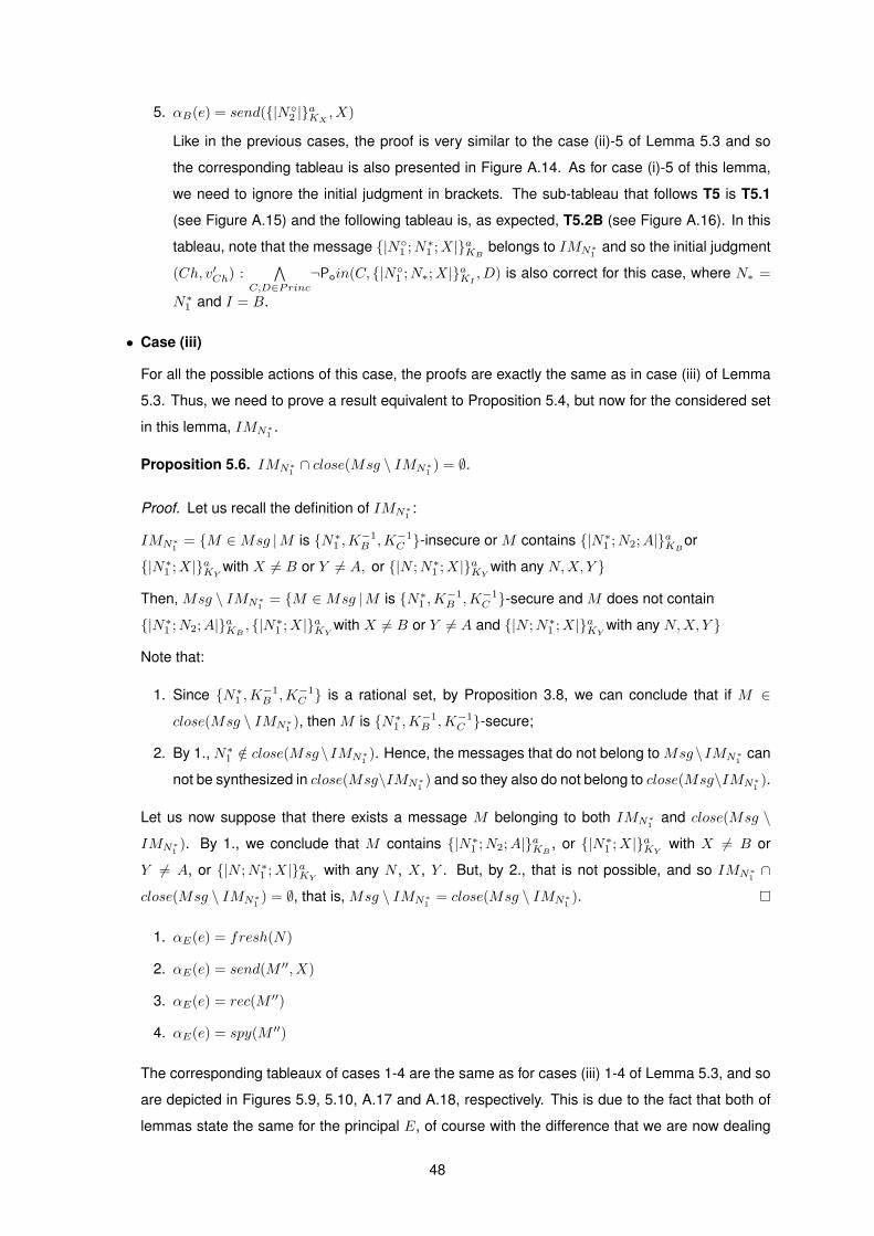
5. αB(e) = send({|N◦2 |}aKX , X)

Like in the previous cases, the proof is very similar to the case (ii)-5 of Lemma 5.3 and so

the corresponding tableau is also presented in Figure A.14. As for case (i)-5 of this lemma,

we need to ignore the initial judgment in brackets. The sub-tableau that follows T5 is T5.1

(see Figure A.15) and the following tableau is, as expected, T5.2B (see Figure A.16). In this

tableau, note that the message {|N◦1 ;N∗1 ;X|}aKB belongs to IMN∗1and so the initial judgment

(Ch, v′Ch) :∧

C,D∈Princ¬Poin(C, {|N◦1 ;N∗;X|}aKI , D) is also correct for this case, where N∗ =

N∗1 and I = B.

• Case (iii)

For all the possible actions of this case, the proofs are exactly the same as in case (iii) of Lemma

5.3. Thus, we need to prove a result equivalent to Proposition 5.4, but now for the considered set

in this lemma, IMN∗1.

Proposition 5.6. IMN∗1∩ close(Msg \ IMN∗1

) = ∅.

Proof. Let us recall the definition of IMN∗1:

IMN∗1= {M ∈Msg |M is {N∗1 ,K−1B ,K−1C }-insecure or M contains {|N∗1 ;N2;A|}aKBor

{|N∗1 ;X|}aKY with X 6= B or Y 6= A, or {|N ;N∗1 ;X|}aKY with any N,X, Y }

Then, Msg \ IMN∗1= {M ∈Msg |M is {N∗1 ,K−1B ,K−1C }-secure and M does not contain

{|N∗1 ;N2;A|}aKB , {|N∗1 ;X|}aKY with X 6= B or Y 6= A and {|N ;N∗1 ;X|}aKY with any N,X, Y }

Note that:

1. Since {N∗1 ,K−1B ,K−1C } is a rational set, by Proposition 3.8, we can conclude that if M ∈

close(Msg \ IMN∗1), then M is {N∗1 ,K−1B ,K−1C }-secure;

2. By 1., N∗1 /∈ close(Msg \IMN∗1). Hence, the messages that do not belong to Msg \IMN∗1

can

not be synthesized in close(Msg\IMN∗1) and so they also do not belong to close(Msg\IMN∗1

).

Let us now suppose that there exists a message M belonging to both IMN∗1and close(Msg \

IMN∗1). By 1., we conclude that M contains {|N∗1 ;N2;A|}aKB , or {|N∗1 ;X|}aKY with X 6= B or

Y 6= A, or {|N ;N∗1 ;X|}aKY with any N , X, Y . But, by 2., that is not possible, and so IMN∗1∩

close(Msg \ IMN∗1) = ∅, that is, Msg \ IMN∗1

= close(Msg \ IMN∗1).

1. αE(e) = fresh(N)

2. αE(e) = send(M ′′, X)

3. αE(e) = rec(M ′′)

4. αE(e) = spy(M ′′)

The corresponding tableaux of cases 1-4 are the same as for cases (iii) 1-4 of Lemma 5.3, and so

are depicted in Figures 5.9, 5.10, A.17 and A.18, respectively. This is due to the fact that both of

lemmas state the same for the principal E, of course with the difference that we are now dealing

48

with the set IMN∗1. Then, in the tableaux in Figures A.17 and A.18, we should substitute IMN by

IMN∗1.

5.4 Rules resultant from the lemmas

In order to incorporate the auxiliary lemmas into the proof of the proposition that states that NSL au-

thenticates the initiator, we need to transform them into rules which can be used in the tableaux. The

rule presented in Figure 5.11 is the translation of Lemma 5.3 and the rule presented in Figure 5.12 is

the translation of Lemma 5.5.

Let (A, vA), (B, vB), (Ch, vCh), (E, vE), E /∈ {A,B} be compatible and M ∈ IMN2 .

(B, v′′B) : fresh(N2)(B, v′′B) < (B, v′B)

(B, v′B) : send({|N1;N2;B|}aKA , A)(B, v′′B) ≤ (B, vB)

(A, vA) : ¬Posend({|N2|}aKB , B)(Ch, vCh) :

∨C,D∈Princ

Poin(C,M,D) | (E, vE) : knows(M)

CLOSED(RN2)

Figure 5.11: Rule (RN2) resultant of Lemma 5.3.

Let (C, v′′C), (Ch, v′′Ch), (E, v′′E), E /∈ {C,B} be compatible and M ∈ IMN∗1.

(B, v′′B) : fresh(N2)(B, v′′B) < (B, v′B)

(B, v′B) : send({|N1;N2;B|}aKZ , Z)(C, v∗C) : fresh(N∗1 )(C, v∗C) < (C, v′′′C )

(C, v′′′C ) : send({|N∗1 ;C|}aKB , B)(C, v∗C) ≤ (C, v′′C)

(Ch, v′′Ch) :∨

C,D∈PrincPoin(C,M,D) | (E, v′′E) : knows(M)

CLOSED(RN∗1

)

Figure 5.12: Rule (RN∗1) resultant of Lemma 5.5.

Like we have already mentioned in subsection 4.2.2, the syntax of local judgments in the local

tableaux system does not include a judgment of the type si ≤ s′i and it should be interpret as si <

s′i ∨ si = s′i.

Since Lemmas 5.3 and 5.5 involve a NSL model, the soundness of the rules in Figures 5.11 and 5.12

is only guaranteed for NSL models.

Proposition 5.7. The rules (RN2) and (RN∗1) are sound for NSL models.

Proof. (RN2): First of all, let us assume the conditions of application of the rule: (A, vA), (B, vB),

(Ch, vCh) and (E, vE), E /∈ {A,B} are compatible and M ∈ IMN2. Let µ be an arbitrary NSL model

and ρ an assignment. Let us assume the premises of the rule, that is:

49

• µ, ρ (B, v′′B) : fresh(N2). Then (†) µ, ξk′′B B fresh(N2), where k′′ = [[(B, v′′B)]]µ,ρ.

• µ, ρ (B, v′′B) < (B, v′B). Then (‡) k′′ < k, where k′ = [[(B, v′B)]]µ,ρ.

• µ, ρ (B, v′B) : send({|N1;N2;B|}aKA , A). Then µ, ξk′

B B send({|N1;N2;B|}aKA , A) and, by (‡),

µ, ξk′′

B B Fsend({|N1;N2;B|}aKA , A). By (†), µ, ξk′′B B (fresh(N2) ∧ Fsend({|N1;N2;B|}aKA , A)).

• µ, ρ (B, v′′B) < (B, vB) ∨ (B, v′′B) = (B, vB). Then k′′ ≤ k, where k = [[(B, vB)]]µ,ρ.

• µ, ρ (A, vA) : ¬Posend({|N2|}aKB , B). Then µ, ξlA A ¬Posend({|N2|}aKB , B), where l = [[(A, vA)]]µ,ρ.

Since we have a premise which is a disjunction, let us split the two hypothesis:

1. µ, ρ (Ch, vCh) :∨

C,D∈PrincPoin(C,M,D). Then, µ, ξnCh Ch

∨C,D∈Princ

Poin(C,M,D), where

n = [[(Ch, vCh]]µ,ρ.

Let ξ be the global state such that |ξB | = k′′. Then µ, ξB B (fresh(N2)∧Fsend({|N1;N2;B|}aKA , A))

and so µ, ξ @B [fresh(N2) ∧ Fsend({|N1;N2;B|}aKA , A)]. Since (A, vA), (B, vB) and (Ch, vCh)

are compatible, let ξ′ be the global state such that |ξ′A| = l, |ξ′B | = k and |ξ′Ch| = n. Then, ξB ⊆ ξ′B ,

µ, ξ′ @A[¬Posend({|N2|}aKB , B)] and µ, ξ′ @Ch[∨

C,D∈PrincPoin(C,M,D)].

Let us divide the rest of the proof in two cases:

(a) ξi ⊆ ξ′i ∀i ∈ {A,E,Ch}. In this case, ξ ⊆ ξ′ and so we can use Lemma 5.3 to conclude that

we can not have µ, ξ′ @Ch[∨


(b) ξi ⊃ ξ′i i ∈ {A,E,Ch}. In this case, let us define the global state ξ′′ such that ξ′′i = ξi and

ξ′′j = ξ′j , j 6= i. Note that ξ ⊆ ξ′′.

i. If i = A, ξ′′A = ξA. Now, if µ, ξ′′ @A[¬Posend({|N2|}aKB , B)], then by Lemma 5.3, µ, ξ′′ 6

@Ch[∧

C,D∈PrincPoin(C,M ′, D)] for every M ′ ∈ IMN2

. Since i 6= Ch, ξ′′Ch = ξ′Ch and so

we have that µ, ξ′ 6 @Ch[∧

C,D∈PrincPoin(C,M,D)]. If µ, ξ′′ @A[Posend({|N2|}aKB , B)],

then µ, ξ @A[Posend({|N2|}aKB , B)]. But by axioms (P1) and (F2), this can not be, since

µ, ξ @B [fresh(N2)] and N2 ∈ cont({|N2|}aKB ).

ii. If i 6= A, ξ′′A = ξ′A and so µ, ξ′′ @A[¬Posend({|N2|}aKB , B)]. By Lemma 5.3 we have

that µ, ξ′′ 6 @Ch[∧

C,D∈PrincPoin(C,M ′, D)] for every M ′ ∈ IMN2 . If i = Ch, then ξ′′Ch =

ξCh ⊃ ξ′Ch and we can not have that µ, ξ′ @Ch[∨

C,D∈PrincPoin(C,M,D)]. If i 6= Ch, then

ξ′′Ch = ξ′Ch and we can immediately conclude that µ, ξ′ 6 @Ch[∧


2. µ, ρ (E, vE) : knows(M). With the appropriate substitutions and adjustments, the proof for this

hypothesis is exactly the same as for hypothesis 1. and so we will abstain from presenting it.

(RN∗1): First of all, let us assume the conditions of application of the rule: (C, v′′C), (Ch, v′′Ch), (E, v′′E), E /∈

{C,B} are compatible and M ∈ IMN∗1. Let µ be an arbitrary NSL model and ρ an assignment. Let us

assume the premises of the rule, that is:

• µ, ρ (B, v′′B) : fresh(N2). Then (†) µ, ξk′′B B fresh(N2), where k′′ = [[(B, v′′B)]]µ,ρ.

50

• µ, ρ (B, v′′B) < (B, v′B). Then (‡) k′′ < k, where k′ = [[(B, v′B)]]µ,ρ.

• µ, ρ (B, v′B) : send({|N1;N2;B|}aKZ , Z). Then µ, ξk′

B B send({|N1;N2;B|}aKZ , Z) and, by (‡),

µ, ξk′′

B B Fsend({|N1;N2;B|}aKZ , Z). By (†), µ, ξk′′B B (fresh(N2) ∧ Fsend({|N1;N2;B|}aKZ , Z)).

Let ζ be the global state such that |ζB | = k′′. Then µ, ζB B (fresh(N2)∧Fsend({|N1;N2;B|}aKA , A))

and so µ, ζ @B [fresh(N2) ∧ Fsend({|N1;N2;B|}aKA , A)].

• µ, ρ (C, v∗C) : fresh(N∗1 ). Then (††) µ, ξk∗B B fresh(N∗1 ), where k∗ = [[(C, v∗C)]]µ,ρ.

• µ, ρ (C, v∗C) < (C, v′′′C ). Then (‡‡) k∗ < k′′′, where k′′′ = [[(C, v′′′C )]]µ,ρ.

• µ, ρ (C, v′′′C ) : send({|N∗1 ;C|}aKB , B). Then µ, ξk′′′

C C send({|N∗1 ;C|}aKB , B) and, by (‡‡),

µ, ξk∗

C C Fsend({|N∗1 ;C|}aKB , B). By (††), we have that µ, ξk∗

C C fresh(N∗1 )∧Fsend({|N∗1 ;C|}aKB , B).

• µ, ρ (C, v∗C) < (C, v′′C) ∨ (C, v∗C) = (C, v′′C). Then k∗ ≤ k∗∗, where k∗∗ = [[(C, v′′C)]]µ,ρ.

Let ξ be the global state such that |ξC | = k∗. Then µ, ξC C fresh(N∗1 ) ∧ Fsend({|N∗1 ;C|}aKB , B)

and so µ, ξ @C [fresh(N∗1 ) ∧ Fsend({|N∗1 ;C|}aKB , B)]. Since (C, v′′C), (Ch, v′′Ch) and (E, v′′E) are

compatible, let ξ′ be the global state such that |ξ′C | = k∗∗, |ξ′Ch| = n and |ξ′E | = l. Then ξC ⊆ ξ′C .

Since we have a premise which is a disjunction, let us split the two hypothesis:

1. µ, ρ (Ch, v′′Ch) :∨

C,D∈PrincPoin(C,M,D). Then, µ, (ξ′Ch)n Ch

∨C,D∈Princ

Poin(C,M,D) and so

µ, ξ′ @Ch[∨


Let us divide the rest of the proof in two cases:

(a) ξi ⊆ ξ′i ∀i ∈ {B,Ch,E}. In this case, ξ ⊆ ξ′ and so we can use Lemma 5.5 to conclude that

we can not have µ, ξ′ @Ch[∨


(b) ξi ⊃ ξ′i i ∈ {A,E,Ch}. In this case, let us define the global state ξ′′ such that ξ′′i = ξi and

ξ′′j = ξ′j , j 6= i. Note that ξ ⊆ ξ′′.

By lemma 5.5, µ, ξ′′ 6 @Ch[∧

C,D∈PrincPoin(C,M ′, D)], for every M ′ ∈ IMN∗1

.

i. If i = Ch, ξ′′Ch = ξCh. Then, µ, ξ 6 @Ch[∧

C,D∈PrincPoin(C,M ′, D)] for every M ′ ∈ IMN∗1

,

and since ξCh ⊃ ξ′Ch, we can not have µ, ξ′ @Ch[∨


ii. If i 6= Ch, ξ′′Ch = ξ′Ch and so µ, ξ′ 6 @Ch[∧

C,D∈PrincPoin(C,M ′, D)] for every M ′ ∈ IMN∗1

.

2. µ, ρ (E, v′′E) : knows(M). With the appropriate substitutions and adjustments, the proof for this

hypothesis is exactly the same as for hypothesis 1. and so we will abstain from presenting it.

As was mentioned in Section 4.3, we can easily state and prove a result equivalent to Proposition

4.13 for NSL models and a version of T ′ augmented with the rules in Figures 5.1, 5.2, 5.11 and 5.12.

51

5.5 Authentication property for NSL

The next proposition is the main result of this chapter, that guarantees that in a NSL protocol the initiator

authenticates the responder.

Proposition 5.8. NSL |= authResp,Init,3B,A (A,B,N1, N2) for A ∈ Princ, B ∈ Hon and N1 and N2 arbitrary

distinct nonces.

Proof. Let us recall that considering an honest principal B, authResp,Init,3B,A (A,B,N1, N2) corresponds to

@B [roleRespB (A,B,N1, N2)]⇒ @A[Posend({|N2|}aKB , B)].

Thus, to prove this result we will resort to Proposition 4.13. Let us separate the proof in two possible

scenarios:

(i) A ∈ Hon:

The corresponding tableau to prove this case is T(i) depicted in Figure A.19. In order to apply

proposition 4.13 we need to assume apriori that (A, vA) and (B, vB) are compatible. Regarding

the tableau, it is very simple and the only observations worth making are that since (B, vB) is syn-

chronized with (Ch, vCh), they are compatible and since we have (Ch, vCh) : Pin(X, {|N2|}aKB , B)

and {|N2|}aKB ∈ IMN2 , then (Ch, vCh) :∨

C,D∈PrincPoin(C,M,D), with M = {|N2|}aKB , and so the

rule (RN2) can be applied to close the tableau.

(ii) A = Z:

The corresponding tableau to prove this case is T(ii) depicted in Figure A.20. In order to apply

proposition 4.13, we need to assume apriori that (B, vB) and (Z, vZ) are compatible.

In T(ii) we divide the tableau in two branches:

1. X = Z

This branch is followed by sub-tableau T(ii).1 (see Figure A.21), in which the initial hypothesis

(Z, vZ) : ¬Posend({|N2|}aKB , B) and the compatibility assumption are crucial to close this

branch.

2. X = C /∈ {B,Z}

We assume that C 6= B because in protocol models no honest principal sends messages to

himself. This branch is followed by sub-tableau T(ii).2 depicted in Figure A.22. In this sub-

tableau, note that (C, v′C) is synchronized with (Ch, v′′Ch), which means they are compatible,

and also that we have (Ch, v′′Ch) : Pin(X, {|N∗1 ;N2;B|}aKC , C), with {|N∗1 ;N2;B|}aKC ∈ IMN∗1.

Then (Ch, v′′Ch) :∨

C,D∈PrincPoin(C,M,D), with M = {|N∗1 ;N2;B|}aKC , and so the rule (RN∗1

)

can be applied to close the tableau.

52

Chapter 6

Message-origin authentication

In this chapter, we describe the TTP and DS models [2] and their transformations - TTP’ and DS*,

but we do not focus on the equivalence of TTP and DS* and of DS and TTP’. Our only purpose is to

prove for each model, individually, the satisfaction of message-origin authentication. Message-origin

authentication is ensuring that a message supposed to come from an agent was really originated by that

agent.

6.1 TTP: Trusted Third Party logging

TTP is an extended model of the CB model of Section 3.2 with an additional communication channel

T , controlled by a trusted third party. Hence, principals can choose to send or receive messages either

through the public channel or through the channel T . Messages sent through T are logged by the trusted

third party, who issues evidence of their origin to the recipients. This way, for all principals, the sets of

actions and state propositions are augmented with actions for communicating with T and propositions

that provide evidence of origin for messages received from T , respectively.

The network signature 〈Princ,Num〉 is fixed, as it was in Section 3.2. The signature ΣTTP is the

tuple 〈Princ ] {Ch, T}, Act, Prop〉 such that for each A ∈ Princ, for Ch and for T we have:

• ActA = {send(M,B), rec(M), spy(M), fresh(X), sendT (M,B), recT (B,M), spyT (B,M)}, where:

– sendT (M,B): sending the message M to principal B via T ;

– recT (B,M): receiving from T the message M originated from principal B;

– spyT (B,M): eavesdropping in T the message M originated from principal B.

• PropA = {knows(M), evid(B,M)}, where:

– evid(B,M): evidence obtained from T that the message M was originated from principal B.

• ActT = ActCh = {in(A,M,B), out(A,M,B), leak}

• PropT = PropCh = ∅

53

Let LTTP denote the DTL language over ΣTTP . The TTP models are the interpretation structures over

ΣTTP that satisfy the following axiomatization:

• (F1-F2), (C1-C4), (P1-P6) and (H);

• Knowledge axiom: Let µ be a TTP model, A ∈ Princ and ξA a non-empty local state of A.

(KT) µ, ξA A knows(M) ⇔ M ∈ close({M ′ |µ, ξA A (Yknows(M ′) ∨ rec(M ′) ∨ spy(M ′) ∨

fresh(M ′) ∨ (∨

B∈Princ(recT (B,M) ∨ spyT (B,M))))})

This axiom replaces axiom (K) of the CB model and properties (K1-K7) also follow from (KT) as

well as the following:

(KT1) @A[recT (B,M)⇒ knows(M)]

(KT2) @A[spyT (B,M)⇒ knows(M)]

• Channel Axioms for T : Let A,B ∈ Princ and M ∈Msg.

(T1) @T [in(A,M,B)�A sendT (M,B)]

(T2) @T [out(A,M,B)⇒ Pin(A,M,B)]

(T3) @T [out(A,M,B)�B recT (A,M)]

(T4) @T [leak ⇒∨

B∈Princc©B [T ]]

• Axioms for the interaction of principals with T : Let A,B ∈ Princ, M ∈ Msg and X ∈ Nonces ]

SymK ] PrivK.

(PT1) @A[sendT (M,B)⇒ Y(knows(M) ∧ knows(B))]

(PT2) @A[sendT (M,B)�T in(A,M,B)]

(PT3) @A[recT (B,M)�T out(B,M,A)]

(PT4) @A[spyT (B,M)�T (leak ∧ P(∨

C∈Princin(B,M,C)))]

(PT5) @A[fresh(X)⇒ ¬ c©T [>]]

• Evidence Axiom: Let A,B ∈ Princ and M ∈Msg.

(E) @A[evid(B,M)⇔ PorecT (B,M)]

• Honesty axiom for interaction with T : Let A ∈ Princ.

(HT) @A[¬spyT (B,M)], for every B ∈ Princ and message M ∈Msg

This axiom is equivalent to axiom (H), but for channel T , and it simply states that honest principals

do not spy messages through T .

The next proposition states that TTP fulfills the message-origin authentication, in the sense that if a

principal receives evidence of the origin of a message he received via the channel T , then that evidence

is correct.

Proposition 6.1. TTP � @A[evid(B,M)]⇒ @B [PosendT (M,A)] for A,B ∈ Princ and M ∈Msg.

54

Proof. The proof for this proposition is the corresponding closed tableau TTTP1 depicted in Figure B.1.

Since we are checking if TTP entails a global implication, we resort to Proposition 4.13. Hence, we

have to assume apriori that (A, vA) and (B, vB) are compatible. Both of the branches in TTTP1 are

followed by tableau TTTP1.1 depicted in Figure B.2. In this sub-tableau, one of its branches is closed

by rule (¬COMP), which is possible by the compatibility assumption established in the beginning, and

the other branch is closed by the initial hypothesis that B did not send M to A through T .

6.2 TTP’ models

TTP’ is a transformation of the TTP model, in which we relax the original model so that the intruder

can divert each message sent to the logged channel T to a different recipient. Being so, we need to

augment the TTP signature with the additional action of diverting a message dvtT and so ΣTTP ′ =

〈Princ ] {Ch, T}, Act, Prop〉 is such that for each A ∈ Princ, for Ch and for T we have:

• ActA = {send(M,B), rec(M), spy(M), fresh(X), sendT (M,B), recT (B,M), spyT (B,M),

dvtT (B,M,C)}, where:

– dvtT (B,M,C): diverting to principal C the message M originated in principal B.

• PropA = {knows(M), evid(B,M)}

• ActT = ActCh = {in(A,M,B), out(A,M,B), leak}

• PropT = PropCh = ∅

Let LTTP ′ denote the DTL language over ΣTTP ′ . The TTP’ models are the interpretation structures

over ΣTTP ′ that satisfy the following axiomatization:

• (F1-F2), (C1-C4), (P1-P6), (H), (T2-T4), (PT1-PT5), (E), (KT) and (HT);

• Replacement / Additional axioms: Let B,C ∈ Princ and M ∈Msg.

(T1’) @T [in(B,M,C)⇒ ( c©B [sendT (M,C)] ∨ (∨

A∈Princc©A[dvtT (B,M,C)]))]

(PT6) @A[dvtT (B,M,C)⇒ PspyT (B,M)]

(PT7) @A[dvtT (B,M,C)�T in(B,M,C)]

Axiom (T1’) replaces axiom (T1) and (PT6) and (PT7) are the additional axioms that model the

additional action of diverting a message.

The next proposition is the equivalent of Proposition 6.1, but now we can not interpret message-origin

authentication as we did for TTP and so this propositions states that TTP’ fulfills a weaker message-

origin authentication. In this weaker formulation, an agent A can only be sure that if he has obtained

evidence from T that a certain message M originated from an agent B, then it must be the case that

B sent M through T to some agent, but not necessarily to A, and in this last detail lies the difference

between the original formulation of message-origin authentication and this weaker one.

55

Proposition 6.2. TTP ′ � @A[evid(B,M)] ⇒ @B [Po(∨

C∈PrincsendT (M,C))] for A,B ∈ Princ and M ∈

Msg.

Proof. The proof for this proposition is the corresponding closed tableau TTTP’1 depicted in Figure

B.3. Like in Proposition 6.1, we are checking if TTP’ entails a global implication and so we resort to

Proposition 4.13 and fix apriori that (A, vA) and (B, vB) are compatible. This way, we can then use

(¬COMP) to close one of the branches of the sub-tableau TTP’1.1 (see Figure B.4). Also in this sub-

tableau, at the point where we use the derived rule (∨

), we divided the branch in two sub-branches, so

that all the principals are represented:

1. The branch where we consider an honest principal X. To close this branch, axiom (HT) is crucial;

2. The branch in which we consider the intruder Z. This branch continues in the sub-tableau TTP’1.2

(see Figure B.5) and when the rule (∨

) is applied, we consider Y to be any principal. We can then

resort to TTP’1.1 if we substitute A by Y and (T, v′T ) by (T, v′′′T ), as indicated in the tableau, and

so the argument will continue using TTP’1.2 again (with the same substitutions) and so on. This

argument leads to an infinite tableau, which can not be by the infinitary closure rule. The strategy

of resorting to previous tableaux and substituting only certain variables intends to avoid repeating

equal tableaux. But we can apply it only because the substitutions made do not alter in any way

the reasoning and rules used in the tableaux.

6.3 DS: Digital Signatures

DS is a concrete model that is similar to a possible realization of an authentic channel. The communi-

cation takes place through a public channel and with the purpose of message-origin authentication in

mind, principals have to digitally sign their sending messages and their signatures can then be verified

by the recipients. More specifically, a principal A should send M ;A; {|M |}aK−1A

and then, by using the

associated public key KA, the receiver can verify the signature to conclude whether M originated from

A. Taking this into account, it is necessary that every principal possesses a secret, namely a special-

purpose asymmetric key, subject to the key axioms (aKey1-aKey2). We assume that these keys have

to be new, that is, {KA |A ∈ Princ} ∩Num = ∅.

The signature ΣDS is identical to ΣCB , but defined over the augmented network signature

〈Princ,Num+〉, where:

• Num+ = Nonces ] SymK ] PubK+;

• PubK+ = PubK ] {KA |A ∈ Princ}.

Msg+ denotes the set of the messages in the augmented network signature.

Let LDS denote the DTL language over ΣDS . The DS models are the interpretation structures over

ΣDS that satisfy the following axiomatization:

56

• (K), (F1-F2), (C1-C4), (P1-P6), (H), (N), (PK) ;

• Honest Agents Axioms: Let A ∈ Princ.

(NS) @A[¬send(M ′, B)] if M ′ ∈ Msg+ \Msg and M ′ 6= M ;A; {|M |}aK−1A

for some M ∈ Msg and

B ∈ Princ

(NR) @A[¬rec(M ′)] if M ′ ∈ Msg+ \ Msg and M ′ 6= M ;B; {|M |}aK−1B


B ∈ Princ

Axiom (NS) states that an honest principal A only uses his private key for signing messages where

signatures or their associated public/private keys do not occur. (NR) guarantees that an honest

principal A never receives messages that use the special-purpose public/private keys, unless they

are properly signed.

• Intruder Axiom:

(NSZ) @Z [¬send(M ′, A)] if M ′ ∈Msg+ \Msg and M ′ 6= M ;B; {|M |}aK−1B

for some M ∈Msg and

B ∈ Princ

This axioms states that the intruder gains nothing from sending messages that no other honest

principal can receive.

Note that the intruder can still prevent message-origin authentication in DS models: if Z spies a

message M ;A; {|M |}aK−1A

sent by a principal A to a principal B and then forwards it to some principal

C, C will have evidence of the message’s origin, but can not guarantee that it was A that actually sent

it. This is why DS models do not satisfy the original formulation of message-origin authentication.

But before proving the weaker formulation for DS models, we need to formulate the rule presented

in Figure 6.1, that guarantees that if the intruder knows a message M ′ = M ;B; {|M |}aK−1B

, where

M ∈ Msg, then it must be the case that the intruder spied M ′ or that B had already sent M ′ to the

intruder.

This rule was introduced to fulfill the need of applying axiom (K) to the tableaux for the proof of

Proposition 6.4, since this axiom can not be translated by a DTL formula and thus, even less be included

in the judgments of the tableau. In section 4.3, this need led us to create rule (RK). In this case,

according to the context of the proof we need to achieve, rule (RDS) is the consequence of axiom (K)

when applied to the premises in question.

Let M ′ = M ;B; {|M |}K−1B, M ∈Msg.

(Z, vZ) : knows(M ′)

(Z, vZ) : Pospy(M ′) | (B, v∗B) : send(M ′, Z), (B, v∗B) ./ (Ch, v∗Ch) < (Ch, v∗∗Ch) ./ (Z, v′Z) ≤ (Z, vZ)(RDS)

Figure 6.1: Rule (RDS).

Like we have mentioned in previous chapters, the judgment of the type si ≤ s′i should be interpret

as si < s′i ∨ si = s′i.

57

This rule is a consequence of the axiomatization for DS models and so it should only be applied in

this context, since its soundness is only guaranteed for these models.

Proposition 6.3. The rule (RDS) is sound for DS models.

Proof. Let µ be an arbitrary DS model and ρ an assignment. Assume now that (†)µ, ρ (Z, vZ) :

knows(M ′) for M ′ = M ;B; {|M |}K−1B

, with M ∈Msg. Let [[(Z, vZ)]]µ,ρ = k. Then µZ , ξkZ Z knows(M′).

By axiom (K), we conclude that M ′ ∈ close(SPK), where SPK = {M∗ |µZ , ξkZ Z (Yknows(M∗) ∨

rec(M∗)∨ spy(M∗)∨ fresh(M∗))}. Since M ′ ∈ close(SPK), then, by the closure rules of a set, we can

divide the proof in two cases:

1. M ′ /∈ SPK

(a) Let us first suppose that K−1B ∈ SPK.

Let us investigate if µZ , ξkZ Z (Yknows(K−1B ) ∨ rec(K−1B ) ∨ spy(K−1B ) ∨ fresh(K−1B )) is pos-

sible.

We can immediately exclude the case where µZ , ξkZ Z fresh(K−1B ), since K−1B is given to B

in the beginning of the protocol.

We can also exclude the case where µZ , ξkZ Z rec(K−1B ) because axioms (P3), (C2) and

(C1) guarantee that there is a principal C that sent K−1B to Z. We can consider that C is

honest, since if C = Z, that would mean Z sent the message to himself and by axiom (P1),

we would go back to the point where Z knows the message. But if C is honest, then by axiom

(NS), he can not send messages of this form to any principal.

With a similar argument, we conclude that it can not be the case µZ , ξkZ Z spy(K−1B ), since

axioms (P4) and (C1) guarantee that K−1B had to be sent from an honest principal to another

honest principal (since we consider that Z does not spy his own messages), and axiom (NS)

does not allow it.

Then, it must be the case that µZ , ξkZ Z Yknows(K−1B ), this is, µZ , ξk−1Z Z knows(K−1B ). If

we proceed with this argument, we conclude that Z has to know K−1B in the initial state, but

by axiom (akey1), that is not possible and so K−1B /∈ SPK.

(b) Now we have already conclude that K−1B /∈ SPK.

By the closure rules of a set, in order to {|M |}K−1B

be synthesized,K−1B has to belong to SPK.

Since it does not belong, then it is because {|M |}K−1B

already belonged to SPK. Then, by

the synthesis rule of pairing (Definition 3.3), it must be the case that M , B and {|M |}K−1B

all

belong to SPK. Hence, let us investigate if µZ , ξkZ Z (Yknows({|M |}K−1B

)∨rec({|M |}K−1B

)∨

spy({|M |}K−1B

) ∨ fresh({|M |}K−1B

)) is possible.

We can immediately exclude the case where µZ , ξkZ Z fresh({|M |}K−1B

), since {|M |}K−1B

is

not atomic. With the same arguments used in case (a), we can also assume that µZ , ξkZ Z

rec({|M |}K−1B

)∨ spy({|M |}K−1B

) is not possible, since {|M |}K−1B

is not a message of the type

that the honest principals are allowed to send and receive.

58

Thus, once again, we have that µZ , ξkZ Z Yknows({|M |}K−1B

). By definition, µZ , ξk−1Z Z

knows({|M |}K−1B

). By the same reasoning, but now applied to the local state ξk−1Z , we would

have that µZ , ξk−1Z Z Yknows({|M |}K−1B

). If we proceed with this argument, we conclude

that Z knows {|M |}K−1B

in the initial state, which is not possible since by axiom (akey1) he

does not even know K−1B .

2. Now we have already concluded that M ′ ∈ SPK.

Hence, we have that µZ , ξkZ Z (Yknows(M ′) ∨ rec(M ′) ∨ spy(M ′) ∨ fresh(M ′)).

The case where we suppose µZ , ξkZ Z fresh(M ′) can once more be immediately exclude be-

cause M ′ is not atomic.

Thus, we have that µZ , ξkZ Z (Yknows(M ′)∨rec(M ′)∨spy(M ′)). Let us suppose that we now have

µZ , ξkZ Z Yknows(M ′). By definition, µZ , ξk−1Z Z knows(M ′). By the same reasoning, but now

applied to the local state ξk−1Z , we would have that µZ , ξk−1Z Z (Yknows(M ′)∨rec(M ′)∨spy(M ′)).

If we proceed with this argument, we conclude that either Z knows M ′ in the initial state, which

again is not possible, or µZ , ξkZ Z Porec(M′) ∨ Pospy(M ′).

Let us now suppose that µZ , ξkZ Z Porec(M′). By the definition of Po, we have that µZ , ξkZ Z

rec(M ′) or µZ , ξkZ Z Prec(M ′). By axiom (P3), µZ , ξkZ Z c©Ch[∨

C∈Princout(C,M ′, Z)] or µZ , ξmZ Z

c©Ch[∨

C∈Princout(C,M ′, Z)], where m = [[(Z, v′Z)]]µ,ρ and m < k. Then by definition, µCh, ξk

′

Ch Ch∨C∈Princ

out(C,M ′, Z) and last(ξkZ) = last(ξk′

Ch) or last(ξmZ ) = last(ξk′

Ch), where k′ = [[(Ch, v∗∗Ch)]]µ,ρ

and so µ, ρ (Ch, v∗∗Ch) ./ (Z, vZ) or µ, ρ (Ch, v∗∗Ch) ./ (Z, v′Z) < (Z, vZ). By axiom (C2), we

have that there exists k′′ < k′such that µCh, ξk′′

Ch Ch∨

C∈Princin(C,M ′, Z). If we consider k′′ =

[[(Ch, v∗Ch)]]µ,ρ, then by definition µ, ρ (Ch, v∗Ch) < (Ch, v∗∗Ch). Finally, by axiom (C1), we have that

there is a principal C such that µCh, ξk′′

Ch Ch c©C [send(M ′, Z)]. But by axiom (NS), if C 6= B, he

is not allowed to send this message to Z. Then we can only have µCh, ξk′′

Ch Ch c©B [send(M ′, Z)].

By definition, µB , ξk∗

B B send(M ′, Z) and last(ξk′′

Ch) = last(ξk∗

B ), where k∗ = [[(B, v∗B)]]µ,ρand so

µ, ρ (B, v∗B) ./ (Ch, v∗Ch) and µ, ρ (B, v∗B) : send(M ′, Z).

As was mentioned in Section 4.3, we can easily state and prove a result equivalent to Proposition

4.13 for DS models and a version of T ′ augmented with the rule in Figure 6.1.

This next proposition proves that the DS models satisfy a form of message-origin authentication

similar to the one stated for TTP’ in Proposition 6.2. It does not fulfill the original form satisfied by TTP

because, as mentioned above, if a principal A receives a certain message digitally signed by a principal

B, then A can only be sure that some B send the message to some principal and not necessarily to

him.

Proposition 6.4. DS � @A[Porec(M′)] ⇒ @B [Po(

∨C∈Princ

send(M ′, C))] for A,B ∈ Princ, M ∈ Msg

and M ′ = M ;B; {|M |}aK−1B

.

59

Proof. The proof for this proposition is the corresponding closed tableau TDS1 depicted in Figure B.6.

To prove the proposition we resort once more to Proposition 4.13 and so, before we consider the tableau

itself, we have to fix that (A, vA) and (B, vB) are compatible.

The initial judgment (X, 0) : Go(∧

D∈Princ¬send(M ′, D)), X /∈ {B,Z} is a direct consequence of axi-

oms (NS) and (NSZ). It is very important to close branch number 2. in the sub-tableau TDS1.1 (see

Figure B.7), since M ′ = M ;B; {|M |}aK−1B

and so M ′ 6= M ;X; {|M |}aK−1A

, since X 6= B.

Also in the sub-tableau TDS1.1, we consider three branches to represent all principals, consequence

of applying the rule (∨

) in the previous tableau:

1. The branch where we consider the principalB. This branch is followed by sub-tableau TDS1.2 (see

Figure B.8), in which the initial hypothesis (B, vB) : ¬Po(∨

C∈Princsend(M ′, C)) and the compatibility

assumption are crucial to close its sub-branches;

2. The branch in which we consider a principal X, where X represents any honest principal other

than B;

3. The branch where we consider the intruder Z. This branch is followed by the sub-tableau TDS1.3

(see Figure B.9), where we apply rule (RDS). Hence, the branch is divided in two sub-branches:

one where we consider that the intruder spied M ′ and the other one where we consider that B

actually sent M ′ to Z.

In the first sub-branch, the argument is continued by resorting to sub-tableau TDS1.1, but substi-

tuting A by Y and (Ch, v′Ch) by (Ch, v′′′Ch), as indicated in the tableau. The tableaux TDS1.2 and

TDS1.3 follow the argument with the same substitutions and this leads to an infinite tableau, which

can not be by rule (INF).

The second sub-branch is followed by sub-tableau TDS1.4 (see Figure B.10), where the trichotomy

rule is used to conclude that with the initial hypothesis (B, vB) : ¬Po(∨

C∈Princsend(M ′, C)), it can

not be the case that B sent M ′ to Z. Note that the condition (B, v∗B) ./ (Ch, v∗Ch) < (Ch, v∗∗Ch) ./

(Z, v′Z) ≤ (Z, vZ) is crucial to apply the rule (¬COMP) and thus to close the leftmost branch in

this tableau.

6.4 DS* models

The DS* model is obtained from the DS model by changing the way messages are signed. In this

transformed model, if a principal A wishes to send a message M to a recipient B, A must include the

name B as part of the signed message, that is, A sends M ;A; {|B;M |}aK−1A

.

The signature ΣDS∗ is equal to ΣDS , but we denote by LDS∗ the DTL language over ΣDS∗ . The DS*

models are the interpretation structures over ΣDS∗ that satisfy the following axiomatization:

• (K), (F1-F2), (C1-C4), (P1-P6), (H), (N), (PK) ;

60

• Replacement Axioms: Let A ∈ Princ

(NS∗) @A[¬send(M ′, B)], if M ′ ∈ Msg+ \Msg and M ′ 6= M ;A; {|B;M |}aK−1A

for some M ∈ Msg

and B ∈ Princ

(NR∗)@A[¬rec(M ′)] if M ′ ∈ Msg+ \Msg and M ′ 6= M ;B; {|A;M |}aK−1B


B ∈ Princ

(NSZ∗) @Z [¬send(M ′, A)] if M ′ ∈Msg+ \Msg and M ′ 6= M ;B; {|A;M |}aK−1B

for some M ∈Msg

and B ∈ Princ

In order to prove the property of message-origin authentication for DS* models, we first need to

introduce a similar rule to (RDS). This new rule, now formulated for DS* models, is also the consequence

of axiom (K) when applied to these models and the premise in question. It guarantees that if the intruder

knows a message M ′ = M ;B; {|A;M |}aK−1B

, where M ∈Msg, then it must be the case that the intruder

spied the message. Differing from rule (RDS), it can not be the case that B had already sent M ′ to Z,

since in DS* models B can only send M ′ to A, which is the name included in the part of the message

that is signed.

Let M ′ = M ;B; {|A;M |}K−1B, M ∈Msg.

(Z, vZ) : knows(M ′)

(Z, vZ) : Pospy(M ′)(RDS∗)

Figure 6.2: Rule (RDS∗).

This rule is a consequence of the axiomatization for DS* models and so it should only be applied in

this context, since its soundness is only guaranteed for these models.

Proposition 6.5. The rule (RDS∗) is sound for DS∗ models.

Proof. The proof is very similar to the one for the soundness of rule (RDS). Hence, we will only point out

the differences in the proof:

• µ is an arbitrary DS∗model;

• µ satisfies axiom (NS∗), instead of (NS);

• In case (b), the sub-message {|A;M |}K−1B

is the one that can not be synthesized (since K−1B does

not has to belong to SPK);

• In case 2., we conclude by axiom (C1) that there is a principalC such that µCh, ξk′′

Ch Ch c©C [send(M ′,

Z)]. But now axiom (NS∗) does not allow C, whether C is B or not, to send M ′ to Z, and so it can

also not be the case that µZ , ξkZ Z Porec(M′).

• Thus, the final conclusion is just that µZ , ξkZ Z Pospy(M ′).

61

Again, we can easily state and prove a result equivalent to Proposition 4.13 for DS* models and a

version of T ′ augmented with the rule in Figure 6.2.

The next proposition is the equivalent of Proposition 6.1, but for the DS* model, which means that

DS* fulfills the message-origin authentication requirement originally stated for TTP.

Proposition 6.6. DS∗ � @A[Porec(M′)] ⇒ @B [Posend(M ′, A)] for A,B ∈ Princ, M ∈ Msg and M ′ =

M ;B; {|A;M |}aK−1B

.

Proof. The proof for this proposition is the corresponding closed tableau TDS∗1 depicted in Figure

B.11. This proof is very similar to the one of Proposition 6.4 and so we also resort Proposition 4.13 and

we have to establish apriori that (A, vA) and (B, vB) are compatible.

The only details that differ from the proof of Proposition 6.4 are the following:

• In the sub-tableau TDS∗1.1 (see Figure B.12), the initial judgment (†)(X, 0) : Go(¬send(M ′, Y )),

X /∈ {B,Z} ∨ Y 6= A, which is now a direct consequence of axioms (NS∗) and (NSZ∗), is very

important to close branch 2. since M ′ = M ;B; {|A;M |}aK−1B

and so M ′ 6= M ;X; {|A;M |}aK−1A

,

since X 6= B;

• The sub-tableau that follows branch 1. is TDS∗1.2, depicted in Figure B.13;

• The sub-tableau that follows branch 3. is TDS∗1.3 (see Figure B.14), in which we apply rule

(RDS∗). Since the conclusion of the rule is that the intruder spied M ′, the argument is very similar

to leftmost branch in tableau TDS1.3. But now, if we consider Y 6= A, we can immediately close

the tableau by the initial hypothesis (†). If Y = A, we can continue the argument by resorting to

sub-tableau TDS1∗.1, substituting (Ch, v′Ch) by (Ch, v′′′Ch), and since the tableaux TDS1∗.2 and

TDS1∗.3 follow the argument with the same substitution, this also leads to an infinite tableau.

62

Chapter 7

Conclusions

Our main objective was to proof the results in [2] by constructing tableaux proofs. Tableaux proofs

are very detailed and, consequently, very extensive and, at times, difficult to read. This may seem a

disadvantage when comparing to semantic proofs, since these last ones are more immediate and less

confusing. But in this point also lies the advantage of doing tableaux proofs, since the details reassure

us of the correctness of the proofs.

In the original tableaux system defined in [1], the semantics of DTL is defined with no global states.

But our aim was to prove results for the original DTL defined in [2], where the concept of global states

is established. In fact, a local state of an agent can be defined resorting to the notion of global state.

Thus, the reasoning that semantically allows us to conclude that certain local states of different agents

are obtained from the same global state is not possible by the tableaux system. The only judgment that

allows us to relate local states of different agents is the synchronization judgment. But this is not enough

to prove some of the results we were aimed to prove.

The global DTL language in [1] does not include the global implication, which is consistent with the

semantic absent of global states, since the satisfaction of a global implication must be defined at a global

state. Many of the results we wanted to prove are global implications and again, we needed to guarantee

that the local states of the two agents considered in the global implication are obtained from the same

global state.

We established right upfront that we would not enrich the language of the tableaux system to allow

global states and, as a consequence, global implications. This was a possible solution, but this approach

had already been explored and it brought up many difficulties. The solution that we implemented was

the introduction of the concept of compatible local states, that precisely connects the local states of

different agents that are obtained from the same global state. We allowed this extra information to be

incorporated in a meta-level, outside the tableaux system, and we introduced a global rule that allows us

to close branches where the relation between two compatible local states contradicts their compatibility.

Axiom (F2) is stated as a global implication and so we could not include it in the judgments of the

tableau. With the definition of compatibility established, we introduced a rule that incorporates the exact

same information of the axiom, providing that the condition for applying this rule is the compatibility

63

assumption regarding the local states of the two agents considered in the global implication.

The inductive reasoning behind the lemmas of Chapter 5 in also not easy to translate to tableaux,

since, locally, we can not translate the relation between two global states. To prove the main result of

this chapter, there was the need to translate the lemmas into sound rules that could then be applied to

the corresponding tableau for the proof of the main result. But the lemmas state an inductive reasoning

and we can only guarantee relations between local states. Hence, the relations judgments in these

rules were carefully though so that when considered all possible cases for local relations we could still

guarantee the relation between the global states.

Another problem that we had to solve were the axioms that could not be written as a DTL formula.

Namely, the knowledge axioms. If they can not even be translated by a DTL formula, it is impossible to

write them as judgments in the tableaux. For this reason, depending on the results we are proving, we

introduced rules that incorporate only the necessary information guaranteed by the axioms to allow us

to conclude what we need to proceed in the tableaux of the corresponding proof. Namely, we introduced

these kinds of rules for CB models, NS models and NS* models.

The knowledge rule (RK), introduced for the CB models, has a premise that includes an universal

quantifier. Universal quantifiers are not allowed in the DTL language for the tableaux system, since in

a rule they may translate an infinite set of premises or an infinite set of conclusions. In order to apply

in a tableau a rule with a universal quantifier in a premise, the tableau ought to have a judgment with

the premise in question, this is, a judgment also with an universal quantifier. We avoided the use of

universal quantifiers in the tableaux as much as possible. But for this specific case, the quantifier is

crucial to guarantee the soundness of the rule and the premise in question translates an hypothesis of

the result for which the rule was used. If the semantic argument takes advantage of this hypothesis, we

could not apply a similar reasoning without considering the whole hypothesis. In the text, we affirm we

undervalue this detail because, in fact, we found no other solution that allowed us to came to the same

conclusions and that did not disregard the language imposition. But a solution to this problem may be to

enrich the language to allow quantifiers.

We extended the global system with a local rule and a global rule and we only proved its soundness.

The proof of its completeness would be desirable in future work. We also presented some derived

rules, but since they are redundant, it does not affect the completeness of the system. Many of the

remaining rules we introduced were not meant to augment the original tableaux system, since they are

the consequence of specific axiomatizations and thus being sound only for the models that satisfy those

axiomatizations. We should also remark that, when introducing new rules, every information that does

not belong to the language allowed in the tableaux was put outside the premises and conclusions of the

rule, as conditions for applying the rule.

In Chapter 6, we did not study the relationship between TTP and DS* and TTP’ and DS, but what

we have observed is that they satisfy, in pairs, the same formulation of message-origin authentication.

Hence, we have presented an example where an abstract model and a transformation of a concrete

model, or a concrete model and a transformation of an abstract model, offer the same guarantees in

terms of message-origin authentication.

64

We did not have the time to prove all of the results in [2], since it is an extensive article. Nevertheless,

with practically all of these main issues resolved, the present work illustrates that it is not necessary to

enrich the language of the tableaux system to prove the results for the original syntax and semantics of

DTL.

65

66

Appendix A

Tableaux for Chapter 5

A.1 Tableaux for Lemmas 5.3 and 5.5

A.1.1 Tableaux for the base case

TB1

HN∗

(Ch,0):Go(in(X,M,Y )�Xsend(m,Y ))

(X,0):Go(send(M,Y )⇒Y(knows(M)∧knows(Y )))

(B,0):G(fresh(N)⇒Y¬knows(M)), N∈cont(M)

(X,0):Go(knows(M)⇒Goknows(M))

TBN∗

... (E,vE):knows(M)

TB1N∗ RF2

(E,vE):¬knows(M)

ABS

CLOSED

Figure A.1: Tableau TB1 for the proof of the base cases of Lemmas 5.3 and 5.5.

67

... TB1N2

(Ch,vCh):∨

C,D∈PrincPoin(C,M,D)

Po

(Ch,vCh):∨

C,D∈Princin(C,M,D) (Ch,vCh):P(

∨C,D∈Princ

in(C,M,D))∨(Ch,v′Ch)<(Ch,vCh)

(Ch,v′Ch):∨

D∈Princin(X,M,D) (Ch,v′Ch):

∨C,D∈Princ

in(C,M,D)∨ ∨(Ch,vCh):in(X,M,Y ) (Ch,v′Ch):

∨D∈Princ

in(X,M,D)

Go ⇒∨

(Ch,vCh): c©X(send(M,Y )) (Ch,v′Ch):in(X,M,Y )

c© Go ⇒

(X,v′X):send(M,Y ) (Ch,v′Ch): c©X(send(M,Y ))

(Ch,vCh)./(X,v′X) c©

SYM (X,v′X):send(M,Y )

(X,v′X)./(Ch,vCh) (Ch,v′Ch)./(X,v′X)

... SYM

TB1.1 (X,v′X)./(Ch,v′Ch)

...

TB1.1

Figure A.2: Sub-tableau TB1N2 for the proof of the base case of Lemma 5.3.

... TB1N∗1

(Ch,vCh):∨

C,D∈Princin(C,M,D)∨

(Ch,v′Ch):∨

D∈Princin(X,M,D)∨

(Ch,vCh):in(X,M,Y )

Go ⇒

(Ch,vCh): c©X(send(M,Y ))

c©

(X,v′X):send(M,Y )

(Ch,vCh)./(X,v′X)

SYM

(X,v′X)./(Ch,vCh)

...

TB1.1

Figure A.3: Sub-tableau TB1N∗1for the proof of the base case of Lemma 5.5.

68

. . .TB

1.1

Go⇒

(X,v′ X):Y(knows(M

)∧knows(Y

))

Y

(X,v′ X−1):knows(M

)∧knows(Y

)

∧


)

(X,v′ X−1):knows(Y

)

Go⇒

(X,v′ X−1):Go(knows(M

))

Go


)

(X,v′ X−1):G(knows(M

))

1.X

=B

2.X∈SP

Go⇒

RF2

(B,vB):Y¬knows(M

)(X,vX):¬knows(M

)

TR

TR

(B,v′ B)<

(B,vB)

(B,v′ B)=

(B,vB)

(B,vB)<

(B,v′ B)

LSHIF

TCONG

¬COM

P

(B,v′ B−1)<

(B,vB−1)

(B,v′ B):Y¬knows(M

)C

LOS

ED

YY

(B,vB−1):¬knows(M

)(B,v′ B−1):¬knows(M

)

GABS

(B,vB−1):knows(M

)C

LOS

ED

ABS

CLO

SE

D

(X,v′ X)<

(X,vX)

(X,v′ X)=

(X,vX)

(X,vX)<

(X,v′ X)

LSHIF

TSUCC

¬COM

P

(X,v′ X−1)<

(X,vX−1)

(X,v′ X−1)<

(X,v′ X)

CLO

SE

D

MON

G

(X,v′ X−1)<

(X,vX)

(X,v′ X):knows(M

)

GCONG

(X,vX):knows(M

)(X,v′ X):¬knows(M

)

ABS

ABS

CLO

SE

DC

LOS

ED

Figure A.4: Sub-tableau TB1.1 for the proof of the base cases of Lemmas 5.3 and 5.5.

69

A.1.2 Tableaux for cases (i) and(ii)

T3

HN∗

(Ch,v′Ch):∧


′,D)


(I,v′I+1):send({|N◦1 ;I|}aKX

,X)

(I,0):Go(send(m,X)�Chin(I,m,X))

(I,0):Go(fresh(N)⇒knows(N))

(I,0):Go(knows(m)⇒Go(knows(m)))

(I,0):Go(fresh(N)⇒Y¬knows(m)), N∈cont(m)

RS1

(Ch,v′Ch+1):in(I,{|N◦1 ;I|}aKX

,X)

(Ch,v′Ch+1):∨

C,D∈PrincPoin(C,M


RS2 ABS

(Ch,v′Ch+1):in(Y,M ′,W ) CLOSED

RNSLI3

(I,v′I+1):Pfresh(N◦1 )

P

(I,v∗I )<(I,v′I+1)

(I,v∗I ):fresh(N◦1 )

...

T3.1

Figure A.5: Tableau T3 for the proof of cases (i)-3 and (ii)-3 of Lemmas 5.3 and 5.5.

... T3.1

1.N◦1 = N∗ 2.N◦1 6= N∗

(I,v∗I ):fresh(N∗) UNIQ... CLOSED

TBN∗

...

T3.2I

Figure A.6: Sub-tableau T3.1 for the proof of cases (i)-3 and (ii)-3 of Lemma 5.3 and 5.5.

70

... T3.2A

FRESH2

CLOSED

... T3.2BN2

TR

(B,v∗B)<(B,vB) (B,v∗B)=(B,vB) (B,vB)<(B,v∗B)

FRESH1 RH1 FRESH1

CLOSED CLOSED CLOSED... T3.2BN∗1

TR


FRESH1

1.X = A 2.X 6= A

UNIQ RH1

CLOSED CLOSED

FRESH1

CLOSED CLOSED

Figure A.7: Sub-tableaux T3.2A, T3.2BN2 and T3.2BN∗1for the proof of cases (i)-3 and (ii)-3 of Lemmas

5.3 and 5.5.

T4

HN∗

(Ch,v′Ch):∧


′,D)

(Ch,v′Ch):∧

C,D∈Princ¬Poin(C,{|N∗;X|}aKI ,D)


(I,v′I+1):send({|N◦1 ;N◦2 ;I|}

aKX

,X)


(I,0):Go(fresh(N)⇒knows(N))

(I,0):Go(knows(m)⇒Go(knows(m)))

(I,0):Go(fresh(N)⇒Y¬knows(m)), cont(N)∩cont(m)6=∅


∨P∈Princ

out(P,m,A))

(Ch,0):Go(out(Y,m,A)⇒Pin(Y,m,A))

RS1

(Ch,v′Ch+1):in(I,{|N◦1 ;N◦2 ;I|}

aKX

,X)

(Ch,v′Ch+1):∨

C,D∈PrincPoin(C,M


RS2 ABS


RNSLR2

(I,v′I+1):P(fresh(N◦2 )∧Prec({|N◦1 ;X|}

aKI

))

P

(I,v∗I )<(I,v′I+1)

(I,v∗I ):fresh(N◦2 )∧Prec({|N

◦1 ;X|}

aKI

)

∧

(I,v∗I ):fresh(N◦2 )

(I,v∗I ):P(rec({|N◦1 ;X|}

aKI

))

...

T4N


71

. . .T4N∗ 1

1.N◦ 2

=N∗ 1

2.N◦ 26=N∗ 1

(I,v∗ I):fresh(N∗ 1)

2.1.N◦ 1

=N∗ 1

2.2.N◦ 16=

N∗ 1

2.1.1

X=

B∨X

=C

2.1.2

X6=

B∧X6=

C

(a)N

o 2=

N2

(b)N

o 26=

N2

(I,v∗ I):fresh(N

2)

UNIQ

∧C

LOS

ED

(A,vA):fresh(N

2)

(A,vA)Fsend({|N

1;N

2;A|}a KZ,Z

)

. . .

T4.2I

(I,v∗ I):P(rec({|N∗ 1;X|}a KI))

. . .

T4.3

UNIQ

CLO

SE

D. . .

TB

N∗ 1

. . .

T4.1I

Figure A.9: Sub-tableau T4N∗1for the proof of cases (i)-4 and (ii)-4 of Lemma 5.5.

72

... T4N2

1.N◦2 = N2 2.N◦2 6=N2

(I,v∗I ):fresh(N2)

2.1.N◦1 = N2 2.2.N◦1 6= N2

(I,v∗I ):P(rec({|N2;X|}aKI )) UNIQ... CLOSED

T4.3(N2)...

TBN2

...

T4.1I

Figure A.10: Sub-tableau T4N2 for the proof of cases (i)-4 and (ii)-4 of Lemma 5.3.

... T4.1A / T4.2B

FRESH2

CLOSED

... T4.2A

TR

(A,v∗A)<(A,vA) (A,v∗A)=(A,vA) (A,vA)<(A,v∗A)

FRESH1 RH1 FRESH1

CLOSED CLOSED CLOSED

Figure A.11: Sub-tableaux T4.1A, T4.2A and T4.2B for the proof of cases (i)-4 and (ii)-4 of Lemmas 5.3

and 5.5.

... T4.1BN2

TR(B,v∗B)<(B,vB) (B,v∗B)=(B,vB) (B,vB)<(B,v∗B)

FRESH1

1.X = A∧N◦1 = N1 2.X 6= A∨N◦1 6= N1

(Ch,v′Ch+1):in(I,{|N1;N2;A|}aKA ,A) RH1UNIQ CLOSED

CLOSED

FRESH1

CLOSED CLOSED... T4.1BN∗1

TR(B,v∗B)<(B,vB) (B,v∗B)=(B,vB) (B,vB)<(B,v∗B)

FRESH1 RH1 FRESH1CLOSED CLOSED CLOSED

Figure A.12: Sub-tableaux T4.1BN2 and T4.1BN∗1for the proof of cases (i)-4 and (ii)-4 of Lemmas 5.3

and 5.5.

73

... T4.3

P

(I,v∗∗I )<(I,v∗I )

(I,v∗∗I ):rec({|N∗;X|}aKI )

Go ⇒

(I,v∗∗I ): c©Ch(∨

P∈Princout(P,{|N∗;X|}aKI ,I))

c©

(Ch,v∗∗Ch):∨

P∈Princout(P,{|N∗;X|}aKI ,I)

(I,v∗∗I )./(Ch,v∗∗Ch)

SYM

(Ch,v∗∗Ch)./(I,v∗∗I )∨

(Ch,v∗∗Ch):out(Y,{|N∗;X|}aKI,I)

Go ⇒

(Ch,v∗∗Ch):Pin(Y,{|N∗;X|}aKI,I)

P

(Ch,v∗∗∗Ch )<(Ch,v∗∗Ch)

(Ch,v∗∗∗Ch ):in(Y,{|N∗;X|}aKI ,I)∧(Ch,v′Ch):

∧D∈Princ

¬Poin(Y,{|N∗;X|}aKI ,D)∧(Ch,v′Ch):¬Poin(Y,{|N∗;X|}aKI ,I)

¬Po

(Ch,v′Ch):¬in(Y,{|N∗;X|}aKI,I)

(Ch,v′Ch):¬Pin(Y,{|N∗;X|}aKI,I)

DIF

(Ch,v∗∗Ch)<(Ch,v′Ch) (Ch,v′Ch)<(Ch,v∗∗Ch)

DTRANS DTRANS

(Ch,v∗∗∗Ch )<(Ch,v′Ch−1) (I,v∗∗I )<(I,v′I)

MON ¬COMP

(Ch,v∗∗∗Ch )<(Ch,v′Ch) CLOSED

¬P

(Ch,v∗∗∗Ch ):¬in(Y,{|N∗;X|}aKI ,I)

ABS

CLOSED

Figure A.13: Sub-tableau T4.3 for the proof of cases (i)-4 and (ii)-4 of Lemmas 5.3 and 5.5.

74

T5

(Ch,v′Ch):∧


′,D)

(Ch,v′Ch):∧

C,D∈Princ¬Poin(C,|N◦1 ;N∗;X|}

aKI,D)

(E,v′E):¬knows(M ′)[(A,v′A+1):¬Posend({|N2|}aKB ,B)

](I,v′I+1):send({|N◦2 |}

aKX

,X)



∨P∈Princ

out(P,m,A))

(Ch,0):Go(out(Y,m,A)⇒Pin(Y,m,A))

(Ch,0):Go(in(Y,m,A)�Y send(m,B))

RS1

(Ch,v′Ch+1):in(I,{|N◦2 |}aKX

,X)

(Ch,v′Ch+1):∨

C,D∈PrincPoin(C,M


RS2 ABS


RNSLI1

(I,v′I+1):P(rec({|N◦1 ;N◦2 ;X|}

aKI

)∧P(send({|N◦1 ;I|}aKX

,X)∧Pfresh(N◦1 )))

P

(I,v∗I )<(I,v′I+1)

(I,v∗I ):rec({|N◦1 ;N

◦2 ;X|}

aKI

)∧P(send({|N◦1 ;I|}aKX

,X)∧Pfresh(N◦1 ))

∧

(I,v∗I ):rec({|N◦1 ;N

◦2 ;X|}

aKI

)

(I,v∗I ):P(send({|N◦1 ;I|}

aKX

,X)∧Pfresh(N◦1 ))

...

T5.1


75

... T5.1

1.N◦2 = N∗ 2.N◦2 6= N∗

(I,v∗I ):rec({|N◦1 ;N∗;X|}

aKI

) UNIQ

Go ⇒ CLOSED

(I,v∗I ): c©Ch(∨

C∈Princout(C,{|N◦1 ;N∗;X|}

aKI,I))

c©

(Ch,v∗Ch):∨

C∈Princout(C,{|N◦1 ;N∗;X|}

aKI,I)

(I,v∗I )./(Ch,v∗Ch)

SYM

(Ch,v∗Ch)./(I,v∗I )∨

(Ch,v∗Ch):out(Y,{|N◦1 ;N∗;X|}

aKI,I)

Go ⇒

(Ch,v∗Ch):Pin(Y,{|N◦1 ;N∗;X|}

aKI,I)

P

(Ch,v∗∗Ch)<(Ch,v∗Ch)

(Ch,v∗∗Ch):in(Y,{|N◦1 ;N∗;X|}

aKI,I)

...

T5.2I

Figure A.15: Sub-tableau T5.1 for the proof of cases (i)-5 and (ii)-5 of Lemmas 5.3 and 5.5.

... T5.2A

1.N◦1 6= N1 ∨X 6= B 2.N◦1 = N1 ∧X = B... (A,v′A+1):send({|N2|}aKB ,B)

T5.2B ¬Po

(A,v′A+1):¬send({|N2|}aKB ,B)

(A,v′A+1):¬Psend({|N2|}aKB ,B)

ABS

CLOSED

... T5.2B∧(Ch,v′Ch):

∧D∈Princ

¬Poin(Y,|N◦1 ;N∗;X|}aKI,D)∧

(Ch,v′Ch):¬Poin(Y,{|N◦1 ;N∗;X|}aKI,I)

¬Po

(Ch,v′Ch):¬in(Y,{|N◦1 ;N∗;X|}

aKI,I)

(Ch,v′Ch):¬Pin(Y,{|N◦1 ;N∗;X|}

aKI,I)

DIF

(Ch,v∗∗Ch)<(Ch,v′Ch) (Ch,v′Ch)<(Ch,v∗∗Ch)

¬P DTRANS

(Ch,v∗∗Ch):¬in(Y,{|N◦1 ;N∗;X|}

aKI,I) (Ch,v′Ch)<(Ch,v∗Ch−1)

ABS RSHIFT

CLOSED (Ch,v′Ch+1)<(Ch,v∗Ch)

¬COMP

CLOSED

Figure A.16: Sub-tableaux T5.2A and T5.2B for the proof of cases (i)-5 and (ii)-5 of Lemmas 5.3 and

5.5.

76

A.1.3 Tableaux for case (iii)

T8

(Ch,v′Ch):∧


′,D)

(Ch,v′Ch):∧


′′,D), M ′′∈IMN


(E,v′E+1):rec(M ′′)

(E,0):Go(rec(M′′)�Ch

∨P∈Princ

out(P,M ′′,E))

(Ch,0):Go(out(X,M′′,E)⇒Pin(X,M ′′,E))

RS1

(Ch,v′Ch+1):∨

P∈Princout(P,M ′′,E)

(Ch,v′Ch+1):∨

C,D∈PrincPoin(C,M


RS2

(Ch,v′Ch+1):in(Y,M ′,W )

UNIQ

CLOSED

1.M′′ ∈ IMN∗ 2.M′′ /∈ IMN∗∨RK

(Ch,v′Ch+1):out(X,M ′′,E) CLOSED

Go ⇒

(Ch,v′Ch+1):Pin(X,M ′′,E)

P

(Ch,v∗Ch)<(Ch,v′Ch+1)

(Ch,v∗Ch):in(X,M′′,E)∧

(Ch,v′Ch):∧

D∈Princ¬Poin(X,M

′′,D)∧(Ch,v′Ch):¬Poin(X,M

′′,E)

¬Po

(Ch,v′Ch):¬in(X,M′′,E)

(Ch,v′Ch):¬Pin(X,M′′,E)

DIF

(Ch,v∗Ch)<(Ch,v′Ch) (Ch,v′Ch)<(Ch,v∗Ch)

¬P DTRANS

(Ch,v∗Ch):¬in(X,M′′,E) (Ch,v′Ch)<(Ch,v′Ch)

ABS NLOOP

CLOSED CLOSED

Figure A.17: Tableau T8 for the proof of case (iii)-3 of Lemmas 5.3 and 5.5.

77

T9

(Ch,v′Ch):∧

C,D∈Princ¬Po(in(C,M

′,D))

(Ch,v′Ch):∧


′′,D), M ′′∈IMN


(E,v′E+1):spy(M ′′)

(E,0):Go(spy(M′′)�Chleak∧P

∨P,Q∈Princ

out(P,M ′′,Q))

(Ch,0):Go(out(X,M′′,Y )⇒Pin(X,M ′′,Y ))

RS1

(Ch,v′Ch+1):leak∧P∨

P,Q∈Princout(P,M ′′,Q)

∧

(Ch,v′Ch+1):leak

(Ch,v′Ch+1):P∨

P,Q∈Princout(P,M ′′,Q)

(Ch,v′Ch+1):∨

C,D∈PrincPoin(C,M


RS2

(Ch,v′Ch+1):in(Y,M ′,W )

UNIQ

CLOSED

1.M′′ ∈ IMN∗ 2.M′′ /∈ IMN∗

P RK

(Ch,v∗Ch)<(Ch,v′Ch+1) CLOSED

(Ch,v∗Ch):∨

P,Q∈Princout(P,M ′′,Q)∨

(Ch,v∗Ch):∨

Q∈Princout(X,M ′′,Q)∨

(Ch,v∗Ch):out(X,M′′,Y )

Go ⇒

(Ch,v∗Ch):Pin(X,M′′,Y )

P

(Ch,v∗∗Ch)<(Ch,v∗Ch)

(Ch,v∗∗Ch):in(X,M′′,Y )∧

(Ch,v′Ch):∧

D∈Princ¬Poin(X,M

′′,D)∧(Ch,v′Ch):¬Poin(X,M

′′,Y )

¬Po

(Ch,v′Ch):¬in(X,M′′,Y )

(Ch,v′Ch):¬Pin(X,M′′,Y )

DTRANS

(Ch,v∗∗Ch)<(Ch,v′Ch)

¬P

(Ch,v∗Ch):¬in(X,M′′,Y )

ABS

CLOSED

Figure A.18: Tableau T9 for the proof of case (iii)-4 of Lemmas 5.3 and 5.5.

78

79

A.2 Tableaux for Proposition 5.8

T(i)

(B,vB):rec({|N2|}aKB )∧P(send({|N1;N2;B|}aKA ,A)∧P(fresh(N2)∧Prec({|N1;A|}aKB )))

(A,vA):¬Posend({|N2|}aKB ,B)

(B,0):Go(rec(m)�Ch

∨C∈Princ

out(C,m,B))

(Ch,0):Go(out(C,m,B)⇒Pin(C,m,B))

∧

(B,vB):rec({|N2|}aKB )

(B,vB):P(send({|N1;N2;B|}aKA ,A)∧P(fresh(N2)∧Prec({|N1;A|}aKB )))

P

(B,v′B)<(B,vB)

(B,v′B):send({|N1;N2;B|}aKA ,A)∧P(fresh(N2)∧Prec({|N1;A|}aKB ))

∧

(B,v′B):send({|N1;N2;B|}aKA ,A)

(B,v′B):P(fresh(N2)∧Prec({|N1;A|}aKB ))

P

(B,v′′B)<(B,v′B)

(B,v′′B):fresh(N2)∧Prec({|N1;A|}aKB )

∧

(B,v′′B):fresh(N2)

(B,v′′B):Prec({|N1;A|}aKB )

DTRANS

(B,v′′B)<(B,vB−1)

MON

(B,v′′B)<(B,vB)

Go ⇒

(B,vB): c©Ch(∨

C∈Princout(C,{|N2|}aKB ,B))

c©

(Ch,vCh):∨

C∈Princout(C,{|N2|}aKB ,B)

(B,vB)./(Ch,vCh)∨(Ch,vCh):out(X,{|N2|}aKB ,B)

Go ⇒

(Ch,vCh):Pin(X,{|N2|}aKB ,B)

RN2

CLOSED

Figure A.19: Tableau T(i) for the proof of case (i) of Proposition 5.8.

80

T(ii)

(B,vB):rec({|N2|}aKB )∧P(send({|N1;N2;B|}aKZ ,Z)∧P(fresh(N2)∧Prec({|N1;Z|}aKB )))

(Z,vZ):¬Posend({|N2|}aKB ,B)

(Y,0):Go(rec(m)�Ch

∨P∈Princ

out(P,m,Y ))

(Ch,0):Go(out(X,m,Y )⇒Pin(X,m,Y ))

(Ch,0):Go(in(X,m,Y )�Xsend(m,Y ))

¬Po

(Z,vZ):¬send({|N2|}aKB ,B)

(Z,vZ):¬Psend({|N2|}aKB ,B)

∧

(B,vB):rec({|N2|}aKB )

(B,vB):P(send({|N1;N2;B|}aKZ ,Z)∧P(fresh(N2)∧Prec({|N1;Z|}aKB )))

P

(B,v′B)<(B,vB)

(B,v′B):send({|N1;N2;B|}aKZ ,Z)∧P(fresh(N2)∧Prec({|N1;Z|}aKB ))

∧

(B,v′B):send({|N1;N2;B|}aKZ ,Z)

(B,v′B):P(fresh(N2)∧Prec({|N1;Z|}aKB ))

P

(B,v′′B)<(B,v′B)

(B,v′′B):fresh(N2)∧Prec({|N1;Z|}aKB )

∧

(B,v′′B):fresh(N2)

(B,v′′B):Prec({|N1;Z|}aKB )

Go ⇒

(B,vB): c©Ch(∨

P∈Princout(P,{|N2|}aKB ,B))

c©

(Ch,vCh):∨

P∈Princout(P,{|N2|}aKB ,B)

(B,vB)./(Ch,vCh)

SYM

(Ch,vCh)./(B,vB)∨(Ch,vCh):out(X,{|N2|}aKB ,B)

...

T(ii).1

Figure A.20: Tableau T(ii) for the proof of case (ii) of Proposition 5.8.

81

... T(ii).1

Go ⇒

(Ch,vCh):Pin(X,{|N2|}aKB ,B)

P

(Ch,v′Ch)<(Ch,vCh)

(Ch,v′Ch):in(X,{|N2|}aKB ,B)

Go ⇒

(Ch,v′Ch): c©X(send({|N2|}aKB ,B))

c©

(X,v′X):send({|N2|}aKB ,B)

(Ch,v′Ch)./(X,v′X)

SYM

(X,v′X)./(Ch,v′Ch)

1.X = Z 2.X = C /∈ {B,Z}

DIF...

(Z,v′Z)<(Z,vZ) (Z,vZ)<(Z,v′Z)

¬P ¬COMP

(Z,v′Z):¬send({|N2|}aKB ,B) CLOSED

ABS

CLOSED

T(ii).2

Figure A.21: Sub-tableau T(ii).1 for the proof of case (ii) of Proposition 5.8.

82

... T(ii).2

RNSLI1

(C,v′C):P(rec({|N∗1 ;N2;B|}aKC )∧P(send({|N∗1 ;C|}aKB

,B)∧Pfresh(N∗1 )))

P

(C,v′′C)<(C,v′C)

(C,v′′C):rec({|N∗1 ;N2;B|}aKC )∧P(send({|N∗1 ;C|}aKB

,B)∧Pfresh(N∗1 ))

∧

(C,v′′C):rec({|N∗1 ;N2;B|}aKC )

(C,v′′C):P(send({|N∗1 ;C|}aKB

,B)∧Pfresh(N∗1 ))

P

(C,v′′′C )<(C,v′′C)

(C,v′′′C ):send({|N∗1 ;C|}aKB

,B)∧Pfresh(N∗1 )

∧

(C,v′′′C ):send({|N∗1 ;C|}aKB

,B)

(C,v′′′C ):Pfresh(N∗1 )

P

(C,v∗C)<(C,v′′′C )

(C,v∗C):fresh(N∗1 )

DTRANS

(C,v∗C)<(C,v′′C−1)

MON

(C,v∗C)<(C,v′′C)

Go ⇒

(C,v′′C): c©Ch(∨

P∈Princout(P,{|N∗1 ;N2;B|}aKC ,C))

c©

(Ch,v′′Ch):∨

P∈Princout(P,{|N∗1 ;N2;B|}aKC ,C)

(C,v′′C)./(Ch,v′′Ch)∨(Ch,v′′Ch):out(X,{|N

∗1 ;N2;B|}aKC ,C)

Go ⇒

(Ch,v′′Ch):Pin(X,{|N∗1 ;N2;B|}aKC ,C)

RN∗1

CLOSED

Figure A.22: Sub-tableau T(ii).2 for the proof of case (ii) of Proposition 5.8.

83

84

Appendix B

Tableaux for Chapter 6

B.1 TTP

TTTP1

(A,vA):evid(B,M)

(B,vB):¬PosendT (M,A)

(A,0):Go(evid(B,M)⇔PorecT (B,M))

(A,0):Go(recT (B,M)�T out(B,M,A))

(T,0):Go(out(B,M,A)⇒Pin(B,M,A))

(T,0):Go(in(B,M,A)�BsendT (M,A))

Go ⇒

(A,vA):PorecT (B,M)

Po

(A,vA):recT (B,M) (A,vA):PrecT (B,M)

Go ⇒ P

(A,vA): c©T [out(B,M,A)] (A,v′A)<(A,vA)

c© (A,v′A):recT (B,M)

(T,vT ):out(B,M,A) Go ⇒

(A,vA)./(T,vT ) (A,v′A): c©T [out(B,M,A)]

SYM c©

(T,vT )./(A,vA) (T,vT ):out(B,M,A)

... (A,v′A)./(T,vT )

TTTP1.1 SYM

(T,vT )./(A,v′A)

...

TTTP1.1

Figure B.1: Tableau TTTP1 for the proof of Proposition 6.1.

85

... TTTP1.1

Go ⇒

(T,vT ):Pin(B,M,A)

P

(T,v′T )<(T,vT )

(T,v′T ):in(B,M,A)

Go ⇒

(T,v′T ): c©B [sendT (M,A)]

c©

(B,v′B):sendT (M,A)

(T,v′T )./(B,v′B)

¬Po

(B,vB):¬sendT (M,A)

(B,vB):¬PsendT (M,A)

DIF

(B,vB)<(B,v′B) (B,v′B)<(B,vB)

SYM ¬P

(B,v′B)./(T,v′T ) (B,v′B):¬sendT (M,A)

¬COMP ABS

CLOSED CLOSED

Figure B.2: Sub-tableau TTTP1.1 for the proof of Proposition 6.1.

86

B.2 TTP’

TTTP’1

(A,vA):evid(B,M)

(B,vB):¬Po(∨

C∈PrincsendT (M,C))

(A,0):Go(evid(B,M)⇔PorecT (B,M))

(A,0):Go(recT (B,M)�T out(B,M,A))

(T,0):Go(out(B,M,A)⇒Pin(B,M,A))

(T,0):Go(in(B,M,A)⇒( c©B [sendT (M,A)]∨(∨

C∈Princc©C [dvtT (B,M,A)])))

(X,0):Go(dvtT (B,M,A)⇒PspyT (B,M))

(X,0):Go(∧

C∈Princ¬spyT (C,M)), X∈Hon

(Z,0):Go(spyT (B,M)�T (leak∧P (∨

D∈Princin(B,M,D)))

Go ⇒

(A,vA):PorecT (B,M)

Po

(A,vA):recT (B,M) (A,vA):PrecT (B,M)

Go ⇒ P

(A,vA): c©T [out(B,M,A)] (A,v′A)<(A,vA)

c© (A,v′A):recT (B,M)

(T,vT ):out(B,M,A) Go ⇒

(A,vA)./(T,vT ) (A,v′A): c©T [out(B,M,A)]

SYM c©

(T,vT )./(A,vA) (T,vT ):out(B,M,A)

Go ⇒ (A,v′A)./(T,vT )

(T,vT ):Pin(B,M,A) SYM

P (T,vT )./(A,v′A)

(T,v′T )<(T,vT ) Go ⇒

(T,v′T ):in(B,M,A) (T,vT ):Pin(B,M,A)

... P

TTTP′1.1 (T,v′T )<(T,vT )

(T,v′T ):in(B,M,A)

...

TTTP′1.1

Figure B.3: Tableau TTTP’1 for the proof of Proposition 6.2.

87

. . .TT

TP’1

.1Go⇒

(T,v′ T):

c ©B[sendT(M

,A)]∨(

∨C∈Princ

c ©C[dvt T

(B,M,A

)])

∨(T,v′ T):

c ©B[sendT(M

,A)]

(T,v′ T):

∨C∈Princ

c ©C[dvt T

(B,M,A

)]

c ©∨

(B,v′ B):sendT(M

,A)

1.X∈Hon

2.

(T,v′ T):

c ©X[dvt T

(B,M,A

)]···

(T,v′ T):

c ©Z[dvt T

(B,M,A

)]

c ©c ©

(X,vX):dvt T

(B,M,A

)(Z,vZ):dvt T

(B,M,A

)

(T,v′ T)./(X,vX)

(T,v′ T)./(Z,vZ)

Go⇒

Go⇒

(X,vX):PspyT(B,M

)(Z,vZ):PspyT(B,M

)

PP

(X,v′ X)<

(X,vX)

(Z,v′ Z)<

(Z,vZ)

(X,v′ X):spyT(B,M

)(Z,v′ Z):spyT(B,M

)

Go⇒

. . .(X,v′ X):

∧C∈Princ

¬spyT(C,M

)TTTP′ 1.2

∧(X,v′ X):¬spyT(B,M

)

ABS

CLO

SE

D(T,v′ T)./(B,v′ B)

¬Po

(B,vB):

∧C∈Princ

¬sendT(M

,C)

(B,vB):¬P(

∨C∈Princ

sendT(M

,C))

∧(B,vB):¬sendT(M

,A)

DIF

(B,v′ B)<

(B,vB)

(B,vB)<

(B,v′ B)

¬PSYM

(B,v′ B)::

∧C∈Princ

¬sendT(M

,C)

(B,v′ B)./(T,v′ T)

∧¬C

OM

P(B,v′ B):¬sendT(M

,A)

CLO

SE

DABS

CLO

SE

D

Figure B.4: Sub-tableau TTTP’1.1 for the proof of Proposition 6.2.

88

... TTTP’1.2Go ⇒

(Z,v′Z): c©T (leak∧P (∨

D∈Princin(B,M,D)))

c©(T,v′′T ):leak∧P (

∨D∈Princ

in(B,M,D))

(Z,v′Z)./(T,v′′T )

∧(T,v′′T ):leak

(T,v′′T ):P (∨

D∈Princin(B,M,D))

P(T,v′′′T )<(T,v′′T )

(T,v′′′T ):∨

D∈Princin(B,M,D)∨

(T,v′′′T ):in(B,M,Y )

...TTTP′1.1

[{A→Y,(T,v′T )→(T,v′′′T )}]...

TTTP′1.2...

INFCLOSED

Figure B.5: Sub-tableau TTTP’1.2 for the proof of Proposition 6.2.

89

B.3 DS

TDS1

(A,vA):Porec(M′)

(B,vB):¬Po(∨

C∈Princsend(M ′,C))

(A,0):Go(rec(M′)�Ch(

∨C∈Princ

out(C,M ′,A)))

(Ch,0):Go(out(X,M′,A)⇒Pin(X,M ′,A))

(Ch,0):Go(in(X,M′,Y )�Xsend(M

′,Y ))

(X,0):Go(∧

D∈Princ¬send(M ′,D)),X /∈{B,Z}

(Z,0):Go(send(M′,X)⇒Y(knows(M ′)∧knows(X)))

(Z,0):Go(spy(M′)�Ch(leak∧P

∨C,D∈Princ

in(C,M ′,D))

¬Po

(B,vB):¬(∨


(B,vB):¬P(∨


Po

(A,vA):rec(M ′) (A,vA):Prec(M ′)

Go ⇒ P

(A,vA): c©Ch(∨

C∈Princout(C,M ′,A)) (A,v′A)<(A,vA)

c© (A,v′A):rec(M ′)

(Ch,vCh):∨

C∈Princout(C,M ′,A) Go ⇒

(A,vA)./(Ch,vCh) (A,v′A): c©Ch(∨

C∈Princout(C,M ′,A))

SYM c©

(Ch,vCh)./(A,vA) (Ch,vCh):∨

C∈Princout(C,M ′,A)∨

(A,v′A)./(Ch,vCh)

(Ch,vCh):out(X,M′,A) SYM

Go ⇒ (Ch,vCh)./(A,v′A)

(Ch,vCh):Pin(X,M′,A)

∨P (Ch,vCh):out(X,M

′,A)

(Ch,v′Ch)<(Ch,vCh) Go ⇒

(Ch,v′Ch):in(X,M′,A) (Ch,vCh):Pin(X,M

′,A)

... P

TDS1.1 (Ch,v′Ch)<(Ch,vCh)

(Ch,v′Ch):in(X,M′,A)

...

TDS1.1

Figure B.6: Tableau TDS1 for the proof of Proposition 6.4.

90

... TDS1.1Go ⇒

(Ch,v′Ch): c©X(send(M ′,A))

c©(X,vX):send(M ′,A)

(Ch,v′Ch)./(X,vX)

SYM(X,vX)./(Ch,v′Ch)

1. 2.X /∈ {B,Z} 3.(B,v′B):send(M ′,A) · · · Go · · · (Z,vZ):send(M ′,A)

(B,v′B)./(Ch,v′Ch) (X,vX):∧

D∈Princ¬send(M ′,D) (Z,vZ)./(Ch,v′Ch)

...∧ ...

TDS1.2 (X,vX):¬send(M ′,A) TDS1.3ABS

CLOSED

Figure B.7: Sub-tableau TDS1.1 for the proof of Proposition 6.4.

... TDS1.2TR

(B,v′B)<(B,vB) (B,v′B)=(B,vB) (B,vB)<(B,v′B)

¬P ¬∨

¬COMP(B,v′B):¬

∨C∈Princ

send(M ′,C) (B,vB):¬send(M ′,A) CLOSED

¬∨

CONG(B,vB):¬send(M ′,A) (B,v′B):¬send(M ′,A)



91

... TDS1.3Go ⇒

(Z,vZ):Y(knows(M ′)∧knows(A))

Y(Z,vZ−1):knows(M ′)∧knows(A)

∧(Z,vZ−1):knows(M ′)

(Z,vZ−1):knows(A)

SUCC(Z,vZ−1)<(Z,vZ)

RDS(Z,vZ−1):Pospy(M

′) (B,v∗B):send(M ′,Z)

Go ⇒ (B,v∗B)./(Ch,v∗Ch)<(Ch,v∗∗Ch)./(Z,′vZ)≤(Z,vZ)

c©Ch(leak∧P∨

C,D∈Princin(C,M ′,D))

...

c© TDS1.4(Ch,v′′Ch):leak∧P

∨C,D∈Princ

in(C,M ′,D)

(Z,vZ−1)./(Ch,v′′Ch)

SYM(Ch,v′′Ch)./(Z,vZ−1)

∧(Ch,v′′Ch):leak

(Ch,v′′Ch):P∨

C,D∈Princin(C,M ′,D)

P(Ch,v′′′Ch)<(Ch,v′′Ch)

(Ch,v′′′Ch):∨

C,D∈Princin(C,M ′,D)∨

(Ch,v′′′Ch):∨

D∈Princin(X,M ′,D)∨

(Ch,v′′′Ch):in(X,M′,Y )

...TDS1.1

[{A→Y,(Ch,v′Ch)→(Ch,v′′′Ch)}]...

INFCLOSED


TDS1.4TR


¬P CONG ¬COMP(B,v∗B):¬

∨C∈Princ

send(M ′,C) (B,v∗B):¬(∨

C∈Princsend(M ′,C)) CLOSED

¬∨

¬∨

(B,v∗B):¬send(M ′,Z) (B,v∗B):¬send(M ′,Z)



92

B.4 TDS*

TDS∗1

(A,vA):Porec(M′)

(B,vB):¬Po(send(M′,A))

(A,0):Go(rec(M′)�Ch(

∨C∈Princ

out(C,M ′,A)))

(Ch,0):Go(out(X,M′,Y )⇒Pin(X,M ′,Y ))

(Ch,0):Go(in(X,M′,Y )�Xsend(M

′,Y ))

(X,0):Go(¬send(M ′,Y )),X /∈{B,Z}∨Y 6=A

(Z,0):Go(send(M′,A)⇒Y(knows(M ′)∧knows(A)))

(Z,0):Go(spy(M′)�Ch(leak∧P

∨C,D∈Princ

in(C,M ′,D))

¬Po

(B,vB):¬send(M ′,A)

(B,vB):¬P(send(M ′,A))

Po

(A,vA):rec(M ′) (A,vA):Prec(M ′)

Go ⇒ P

(A,vA): c©Ch(∨

C∈Princout(C,M ′,A)) (A,v′A)<(A,vA)

c© (A,v′A):rec(M ′)

(Ch,vCh):∨

C∈Princout(C,M ′,A) Go ⇒

(A,vA)./(Ch,vCh) (A,v′A): c©Ch(∨

C∈Princout(C,M ′,A))

SYM c©

(Ch,vCh)./(A,vA) (Ch,vCh):∨

C∈Princout(C,M ′,A)∨

(A,v′A)./(Ch,vCh)

(Ch,vCh):out(X,M′,A) SYM

Go ⇒ (Ch,vCh)./(A,v′A)

(Ch,vCh):Pin(X,M′,A)

∨P (Ch,vCh):out(X,M

′,A)

(Ch,v′Ch)<(Ch,vCh) Go ⇒

(Ch,v′Ch):in(X,M′,A) (Ch,vCh):Pin(X,M

′,A)

... P

TDS∗1.1 (Ch,v′Ch)<(Ch,vCh)

(Ch,v′Ch):in(X,M′,A)

...

TDS∗1.1

Figure B.11: Tableau TDS∗1 for the proof of Proposition 6.6.

93

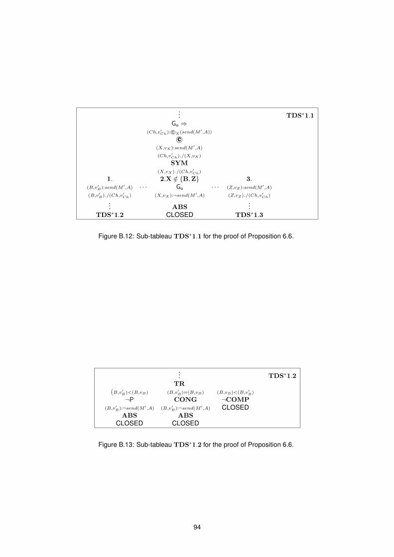
... TDS∗1.1Go ⇒

(Ch,v′Ch): c©X(send(M ′,A))

c©(X,vX):send(M ′,A)

(Ch,v′Ch)./(X,vX)

SYM(X,vX)./(Ch,v′Ch)

1. 2.X /∈ {B,Z} 3.(B,v′B):send(M ′,A) · · · Go · · · (Z,vZ):send(M ′,A)

(B,v′B)./(Ch,v′Ch) (X,vX):¬send(M ′,A) (Z,vZ)./(Ch,v′Ch)

... ABS...

TDS∗1.2 CLOSED TDS∗1.3

Figure B.12: Sub-tableau TDS∗1.1 for the proof of Proposition 6.6.

... TDS∗1.2TR

(B,v′B)<(B,vB) (B,v′B)=(B,vB) (B,vB)<(B,v′B)

¬P CONG ¬COMP(B,v′B):¬send(M ′,A) (B,v′B):¬send(M ′,A) CLOSED



94

... TDS∗1.3Go ⇒

(Z,vZ):Y(knows(M ′)∧knows(A))

Y(Z,vZ−1):knows(M ′)∧knows(A)

∧(Z,vZ−1):knows(M ′)

(Z,vZ−1):knows(A)

SUCC(Z,vZ−1)<(Z,vZ)

RDS∗

(Z,vZ−1):Pospy(M′)

Go ⇒c©Ch(leak∧P

∨C,D∈Princ

in(C,M ′,D))

c©(Ch,v′′Ch):leak∧P

∨C,D∈Princ

in(C,M ′,D)

(Z,vZ−1)./(Ch,v′′Ch)

SYM(Ch,v′′Ch)./(Z,vZ−1)

∧(Ch,v′′Ch):leak

(Ch,v′′Ch):P∨

C,D∈Princin(C,M ′,D)

P(Ch,v′′′Ch)<(Ch,v′′Ch)

(Ch,v′′′Ch):∨

C,D∈Princin(C,M ′,D)∨

(Ch,v′′′Ch):∨

D∈Princin(X,M ′,D)∨

(Ch,v′′′Ch):in(X,M′,Y )

1.Y = A 2.Y 6= A... Go ⇒

TDS∗1.1 (Ch,v′Ch): c©X(send(M ′,A))

[(Ch,v′Ch)→(Ch,v′′′Ch)] c©... (X,vX):send(M ′,A)

INF Go

CLOSED (X,vX):¬send(M ′,A)

ABSCLOSED


95

96

Bibliography

[1] D. Basin, C. Caleiro, J. Ramos, and L. Vigano. Labeled tableaux for distributed temporal

logic. Journal of Logic and Computation, 19(6):1245–1279, 2009.

[2] D. Basin, C. Caleiro, J. Ramos, and L. Vigano. Distributed temporal logic for the analysis of

security protocol models. Theoretical Computer Science, 412(31):4007–4043, 2011.

[3] C. Caleiro, L. Vigano, and D. Basin. Deconstructing alice and bob. Electronic Notes in

Theoretical Computer Science, 135(1):3–22, 2005.

[4] D. R. Stinson. Cryptography Theory and Practice(Third Edition). CRC Press, Inc., 2005.

97

98

Documents

Tableaux for Distributed Temporal Logic · Tableaux for Distributed Temporal Logic Applications to Security Protocols Joana Margarida Simões de Abreu Dissertação para a obtenção