t-Tests for Two Independent Samples - Rutgers Universitymmm431/quant_methods_F14/QM... · 2014-10-30 · 01:830:200:01-04 Spring 2014 t-Tests for Two Independent Samples M Though

Comparing Means:

t-Tests for Two Independent Samples

01:830:200:01-04 Spring 2014


Independent-Measures Designs

• Allows researchers to evaluate the mean difference between

two populations using data from two separate samples.

– The identifying characteristic of the independent-measures or

between-subjects design is the existence of two separate and

independent samples.

– Thus, an independent-measures design can be used to test for mean

differences between two distinct populations (such as men versus

women) or between two different treatment conditions (such as drug

versus no-drug).

01:830:200:01-04 Spring 2014



01:830:200:01-04 Spring 2014



• The independent-measures design is used in situations where

a researcher has no prior knowledge about either of the two

populations (or treatments) being compared.

– In particular, the population means and standard deviations are all

unknown.

– Because the population variances are not known, these values must be

estimated from the sample data.

01:830:200:01-04 Spring 2014


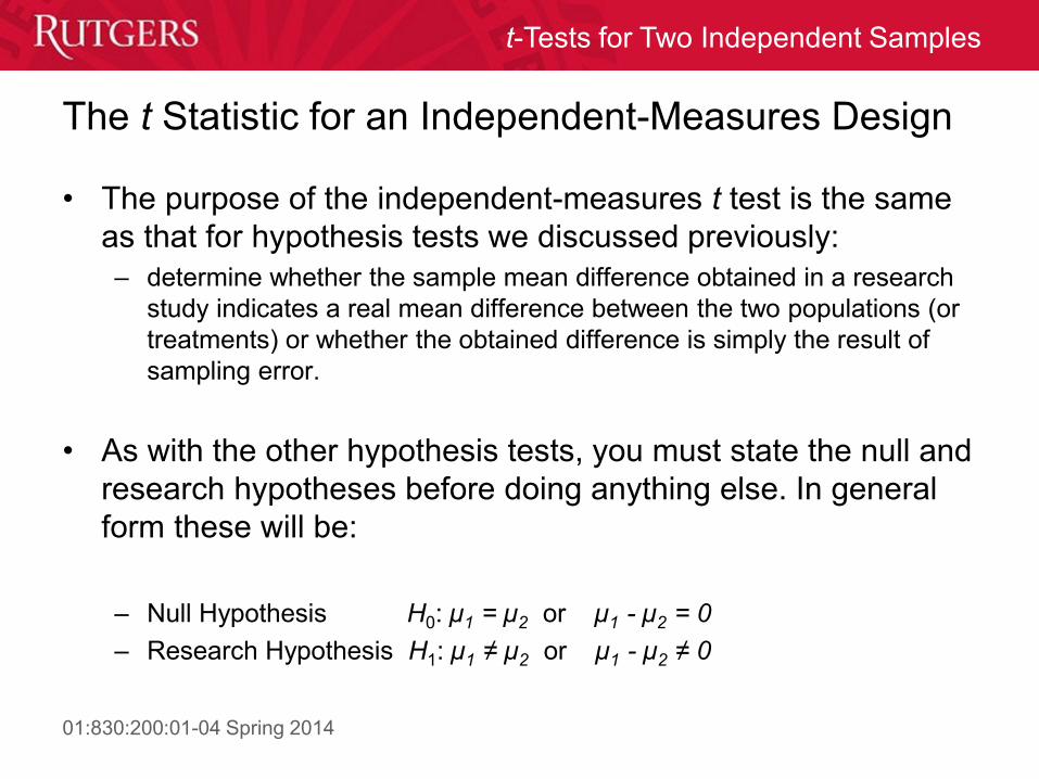
The t Statistic for an Independent-Measures Design

• The purpose of the independent-measures t test is the same

as that for hypothesis tests we discussed previously:

– determine whether the sample mean difference obtained in a research

study indicates a real mean difference between the two populations (or

treatments) or whether the obtained difference is simply the result of

sampling error.

• As with the other hypothesis tests, you must state the null and

research hypotheses before doing anything else. In general

form these will be:

– Null Hypothesis H0: µ1 = µ2 or µ1 - µ2 = 0

– Research Hypothesis H1: µ1 ≠ µ2 or µ1 - µ2 ≠ 0

01:830:200:01-04 Spring 2014


The Independent-Samples t-Test: Steps

1. Use t distribution table to find critical t-value(s) representing

rejection region (denoted using tcrit or tα)

2. Compute t-statistic

– For data in which I give you raw scores, you will have to compute the

sample mean and sample standard deviation for both samples

3. Make a decision: does the t-statistic for your sample fall into

the rejection region?

01:830:200:01-04 Spring 2014


Though the basic form of the t-statistic is similar to that used for

the single-sample test, Some of the details are different.

In particular, note that now we must estimate the standard

deviation and mean for both populations via sample statistics:

t-Statistic for Independent Samples

1 2 1 2

1 1 12 2 2

M M M M

M M M Mt df

s s

?df

1 2?M Ms

01:830:200:01-04 Spring 2014


Sampling Distribution of Difference Between Means

• To compute the t-statistic, we must first characterize the

standard error of the difference between means under the null

hypothesis

• From the variance sum law:

– The variance of the sum or difference of two independent variables is

the sum of their variances.

– Therefore, the standard error of the difference between the means of

two independent samples is the square root of the sum of their squared

standard errors:

2 21 1

2

2

2 22 2 2 1

1

M M M Mn n

1 2 1 2

2 22 1

1

2

2

M M MMn n

01:830:200:01-04 Spring 2014


Estimating the Standard Error of the Difference

Between Means

• Under the null hypothesis, the distributions are equivalent. This means that the population variances for the two samples should be equal: σ2 = σ2

1 = σ22

– This is called homogeneity of variance and it is an important

assumption underlying independent-sample t-tests

• Additionally, since we don’t have the population standard deviations, we estimate the standard error of the mean using the sample standard deviations

• So now we want to estimate a single population variance (σ2) using two estimates (s2

1 & s22). How do we do this?

01:830:200:01-04 Spring 2014



Between Means

• We compute a weighted average called the pooled

variance

• Why?

– Sample statistics computed with more degrees of freedom are less

variable (more reliable). Therefore, when averaging estimates across

samples, we want to give more weight to samples with more degrees of

freedom

2 22 1 1 2 1 2

1 2 1 2

2 ,p

df s df s SSs

d

SS

df dff df

1 1 2 2where 1 and 1df n df n

Note that if df1 = df2, this reduces to a simple average:

2 2 2 22 1 2 1 2

2 2p

dfs dfs s ss

df

01:830:200:01-04 Spring 2014



Between Means

• Finally, we plug the pooled variance (our estimate of the

population variance) into the equation for the standard error of

the difference between means:

1 2

2 2

1 2

, p p

M M

s

n n

ss

2 22 1 1 2 2

1 2

with p

d

d

f s df ss

df f

1 2

2

1 2 1 2

1 1 1 1

M M p ps s s

n n n n

Note that the above reduces to:

01:830:200:01-04 Spring 2014


t-Statistic for Independent Samples

1 2

1 2

M M

MMt df

s

2

1 2

2

1

1 1 1

2

df d df

n n

n

f

n

1 2

2 2

1 2

p p

M Msn n

s s

01:830:200:01-04 Spring 2014


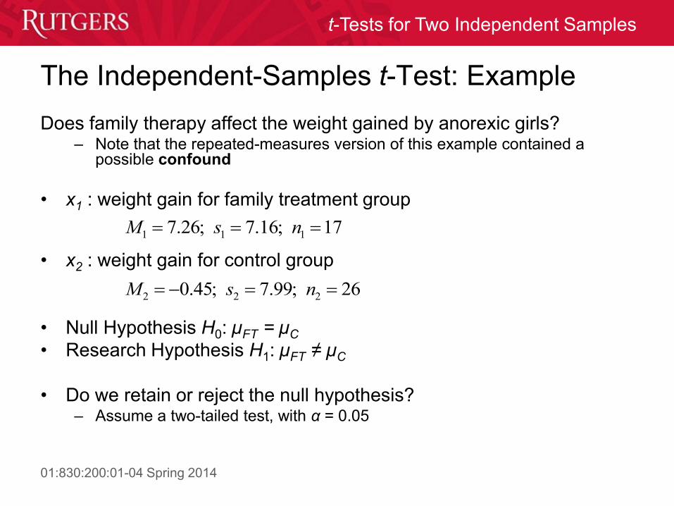
The Independent-Samples t-Test: Example

Does family therapy affect the weight gained by anorexic girls? – Note that the repeated-measures version of this example contained a

possible confound

• x1 : weight gain for family treatment group

• x2 : weight gain for control group

• Null Hypothesis H0: µFT = µC

• Research Hypothesis H1: µFT ≠ µC

• Do we retain or reject the null hypothesis? – Assume a two-tailed test, with α = 0.05

1 11 7.26; 7.16; 17M s n

2 2 20.45; 9 267.9 ;M s n

01:830:200:01-04 Spring 2014










01:830:200:01-04 Spring 2014


Level of significance for one-tailed test

0.25 0.2 0.15 0.1 0.05 0.025 0.01 0.005 0.0005

Level of significance for two-tailed test

df 0.5 0.4 0.3 0.2 0.1 0.05 0.02 0.01 0.001

1 1.000 1.376 1.963 3.078 6.314 12.706 31.821 63.657 636.619

2 0.816 1.061 1.386 1.886 2.920 4.303 6.965 9.925 31.599

3 0.765 0.978 1.250 1.638 2.353 3.182 4.541 5.841 12.924

4 0.741 0.941 1.190 1.533 2.132 2.776 3.747 4.604 8.610

5 0.727 0.920 1.156 1.476 2.015 2.571 3.365 4.032 6.869

6 0.718 0.906 1.134 1.440 1.943 2.447 3.143 3.707 5.959

7 0.711 0.896 1.119 1.415 1.895 2.365 2.998 3.499 5.408

8 0.706 0.889 1.108 1.397 1.860 2.306 2.896 3.355 5.041

9 0.703 0.883 1.100 1.383 1.833 2.262 2.821 3.250 4.781

10 0.700 0.879 1.093 1.372 1.812 2.228 2.764 3.169 4.587

11 0.697 0.876 1.088 1.363 1.796 2.201 2.718 3.106 4.437

12 0.695 0.873 1.083 1.356 1.782 2.179 2.681 3.055 4.318

13 0.694 0.870 1.079 1.350 1.771 2.160 2.650 3.012 4.221

14 0.692 0.868 1.076 1.345 1.761 2.145 2.624 2.977 4.140

15 0.691 0.866 1.074 1.341 1.753 2.131 2.602 2.947 4.073

16 0.690 0.865 1.071 1.337 1.746 2.120 2.583 2.921 4.015

17 0.689 0.863 1.069 1.333 1.740 2.110 2.567 2.898 3.965

18 0.688 0.862 1.067 1.330 1.734 2.101 2.552 2.878 3.922

19 0.688 0.861 1.066 1.328 1.729 2.093 2.539 2.861 3.883

20 0.687 0.860 1.064 1.325 1.725 2.086 2.528 2.845 3.850 21 0.686 0.859 1.063 1.323 1.721 2.080 2.518 2.831 3.819

22 0.686 0.858 1.061 1.321 1.717 2.074 2.508 2.819 3.792

23 0.685 0.858 1.060 1.319 1.714 2.069 2.500 2.807 3.768

24 0.685 0.857 1.059 1.318 1.711 2.064 2.492 2.797 3.745

25 0.684 0.856 1.058 1.316 1.708 2.060 2.485 2.787 3.725 26 0.684 0.856 1.058 1.315 1.706 2.056 2.479 2.779 3.707

27 0.684 0.855 1.057 1.314 1.703 2.052 2.473 2.771 3.690

28 0.683 0.855 1.056 1.313 1.701 2.048 2.467 2.763 3.674

29 0.683 0.854 1.055 1.311 1.699 2.045 2.462 2.756 3.659

30 0.683 0.854 1.055 1.310 1.697 2.042 2.457 2.750 3.646 40 0.681 0.851 1.050 1.303 1.684 2.021 2.423 2.704 3.551

50 0.679 0.849 1.047 1.299 1.676 2.009 2.403 2.678 3.496

100 0.677 0.845 1.042 1.290 1.660 1.984 2.364 2.626 3.390

t-Distribution Table

Two-tailed test

One-tailed test

α

t

α/2 α/2

t -t

01:830:200:01-04 Spring 2014



0.25 0.2 0.15 0.1 0.05 0.025 0.01 0.005 0.0005


df 0.5 0.4 0.3 0.2 0.1 0.05 0.02 0.01 0.001

1 1.000 1.376 1.963 3.078 6.314 12.706 31.821 63.657 636.619

2 0.816 1.061 1.386 1.886 2.920 4.303 6.965 9.925 31.599

3 0.765 0.978 1.250 1.638 2.353 3.182 4.541 5.841 12.924

4 0.741 0.941 1.190 1.533 2.132 2.776 3.747 4.604 8.610

5 0.727 0.920 1.156 1.476 2.015 2.571 3.365 4.032 6.869

6 0.718 0.906 1.134 1.440 1.943 2.447 3.143 3.707 5.959

7 0.711 0.896 1.119 1.415 1.895 2.365 2.998 3.499 5.408

8 0.706 0.889 1.108 1.397 1.860 2.306 2.896 3.355 5.041

9 0.703 0.883 1.100 1.383 1.833 2.262 2.821 3.250 4.781

10 0.700 0.879 1.093 1.372 1.812 2.228 2.764 3.169 4.587

11 0.697 0.876 1.088 1.363 1.796 2.201 2.718 3.106 4.437

12 0.695 0.873 1.083 1.356 1.782 2.179 2.681 3.055 4.318

13 0.694 0.870 1.079 1.350 1.771 2.160 2.650 3.012 4.221

14 0.692 0.868 1.076 1.345 1.761 2.145 2.624 2.977 4.140

15 0.691 0.866 1.074 1.341 1.753 2.131 2.602 2.947 4.073

16 0.690 0.865 1.071 1.337 1.746 2.120 2.583 2.921 4.015

17 0.689 0.863 1.069 1.333 1.740 2.110 2.567 2.898 3.965

18 0.688 0.862 1.067 1.330 1.734 2.101 2.552 2.878 3.922

19 0.688 0.861 1.066 1.328 1.729 2.093 2.539 2.861 3.883

20 0.687 0.860 1.064 1.325 1.725 2.086 2.528 2.845 3.850 21 0.686 0.859 1.063 1.323 1.721 2.080 2.518 2.831 3.819

22 0.686 0.858 1.061 1.321 1.717 2.074 2.508 2.819 3.792

23 0.685 0.858 1.060 1.319 1.714 2.069 2.500 2.807 3.768

24 0.685 0.857 1.059 1.318 1.711 2.064 2.492 2.797 3.745

25 0.684 0.856 1.058 1.316 1.708 2.060 2.485 2.787 3.725 26 0.684 0.856 1.058 1.315 1.706 2.056 2.479 2.779 3.707

27 0.684 0.855 1.057 1.314 1.703 2.052 2.473 2.771 3.690

28 0.683 0.855 1.056 1.313 1.701 2.048 2.467 2.763 3.674

29 0.683 0.854 1.055 1.311 1.699 2.045 2.462 2.756 3.659

30 0.683 0.854 1.055 1.310 1.697 2.042 2.457 2.750 3.646 40 0.681 0.851 1.050 1.303 1.684 2.021 2.423 2.704 3.551

50 0.679 0.849 1.047 1.299 1.676 2.009 2.403 2.678 3.496

100 0.677 0.845 1.042 1.290 1.660 1.984 2.364 2.626 3.390


Two-tailed test

One-tailed test

α

t

α/2 α/2

t -t

01:830:200:01-04 Spring 2014


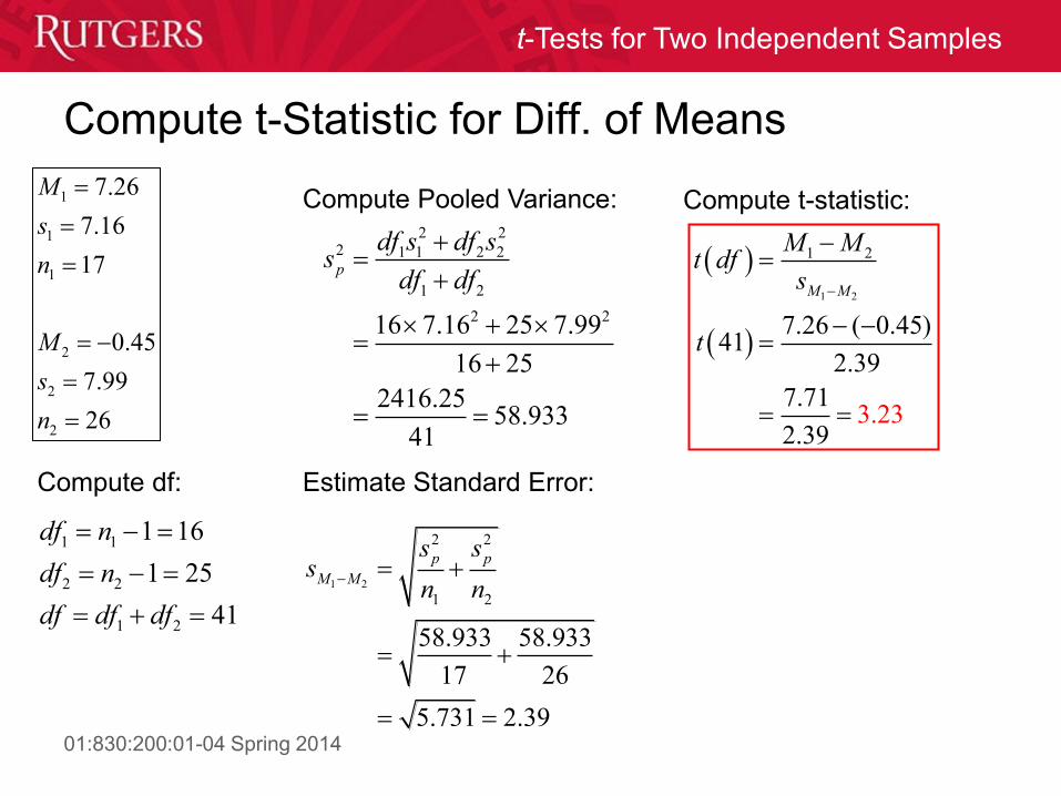
Compute t-Statistic for Diff. of Means

1

2

2

2

1

1

7.26

7.16

0.45

7

17

99

26

.

M

s

n

M

s

n

2

1

1 2

2

1 1 16

1 25

41

n

n

df

d

df

f df

f

d

Compute Pooled Variance: 2 2

2 1 1 2 2

1 2

2 27.16 7.99

16 25

2416.2558.933

4

1 2

1

6 5

p

df s df ss

ddf f

Compute df: Estimate Standard Error:

1 2

2 2

21

58.933 58.9

17 26

5.7

3

31

3

2.39

p p

M M

s ss

n n

Compute t-statistic:

1 2

1 2

7.26 ( 0.45)

2.39

7.71

2.

4

393.

1

23

M M

t dfs

t

M M

01:830:200:01-04 Spring 2014


The Independent-Samples t-Test: A Full Example

Return to our original hypothesis testing example (exam scores). – This time, assume that we randomly assigned students into the courses of two

different instructors (Dr. M & Dr. K) and that do not know the population mean or SD for either class

• x1 : sample scores from Dr. M’s class

• x2 : sample scores from Dr. K’s class

• Null Hypothesis H0: µK = µM

• Research Hypothesis H1: µK ≠ µM

• Do we accept or reject the null hypothesis? – Assume a two-tailed test, with α = 0.05

2 {74,67,69,77,84}x

1 {65,70,71,63,69}x

01:830:200:01-04 Spring 2014










01:830:200:01-04 Spring 2014



0.25 0.2 0.15 0.1 0.05 0.025 0.01 0.005 0.0005


df 0.5 0.4 0.3 0.2 0.1 0.05 0.02 0.01 0.001

1 1.000 1.376 1.963 3.078 6.314 12.706 31.821 63.657 636.619

2 0.816 1.061 1.386 1.886 2.920 4.303 6.965 9.925 31.599

3 0.765 0.978 1.250 1.638 2.353 3.182 4.541 5.841 12.924

4 0.741 0.941 1.190 1.533 2.132 2.776 3.747 4.604 8.610

5 0.727 0.920 1.156 1.476 2.015 2.571 3.365 4.032 6.869

6 0.718 0.906 1.134 1.440 1.943 2.447 3.143 3.707 5.959

7 0.711 0.896 1.119 1.415 1.895 2.365 2.998 3.499 5.408

8 0.706 0.889 1.108 1.397 1.860 2.306 2.896 3.355 5.041

9 0.703 0.883 1.100 1.383 1.833 2.262 2.821 3.250 4.781

10 0.700 0.879 1.093 1.372 1.812 2.228 2.764 3.169 4.587

11 0.697 0.876 1.088 1.363 1.796 2.201 2.718 3.106 4.437

12 0.695 0.873 1.083 1.356 1.782 2.179 2.681 3.055 4.318

13 0.694 0.870 1.079 1.350 1.771 2.160 2.650 3.012 4.221

14 0.692 0.868 1.076 1.345 1.761 2.145 2.624 2.977 4.140

15 0.691 0.866 1.074 1.341 1.753 2.131 2.602 2.947 4.073

16 0.690 0.865 1.071 1.337 1.746 2.120 2.583 2.921 4.015

17 0.689 0.863 1.069 1.333 1.740 2.110 2.567 2.898 3.965

18 0.688 0.862 1.067 1.330 1.734 2.101 2.552 2.878 3.922

19 0.688 0.861 1.066 1.328 1.729 2.093 2.539 2.861 3.883

20 0.687 0.860 1.064 1.325 1.725 2.086 2.528 2.845 3.850 21 0.686 0.859 1.063 1.323 1.721 2.080 2.518 2.831 3.819

22 0.686 0.858 1.061 1.321 1.717 2.074 2.508 2.819 3.792

23 0.685 0.858 1.060 1.319 1.714 2.069 2.500 2.807 3.768

24 0.685 0.857 1.059 1.318 1.711 2.064 2.492 2.797 3.745

25 0.684 0.856 1.058 1.316 1.708 2.060 2.485 2.787 3.725 26 0.684 0.856 1.058 1.315 1.706 2.056 2.479 2.779 3.707

27 0.684 0.855 1.057 1.314 1.703 2.052 2.473 2.771 3.690

28 0.683 0.855 1.056 1.313 1.701 2.048 2.467 2.763 3.674

29 0.683 0.854 1.055 1.311 1.699 2.045 2.462 2.756 3.659

30 0.683 0.854 1.055 1.310 1.697 2.042 2.457 2.750 3.646 40 0.681 0.851 1.050 1.303 1.684 2.021 2.423 2.704 3.551

50 0.679 0.849 1.047 1.299 1.676 2.009 2.403 2.678 3.496

100 0.677 0.845 1.042 1.290 1.660 1.984 2.364 2.626 3.390


Two-tailed test

One-tailed test

α

t

α/2 α/2

t -t

01:830:200:01-04 Spring 2014



0.25 0.2 0.15 0.1 0.05 0.025 0.01 0.005 0.0005


df 0.5 0.4 0.3 0.2 0.1 0.05 0.02 0.01 0.001

1 1.000 1.376 1.963 3.078 6.314 12.706 31.821 63.657 636.619

2 0.816 1.061 1.386 1.886 2.920 4.303 6.965 9.925 31.599

3 0.765 0.978 1.250 1.638 2.353 3.182 4.541 5.841 12.924

4 0.741 0.941 1.190 1.533 2.132 2.776 3.747 4.604 8.610

5 0.727 0.920 1.156 1.476 2.015 2.571 3.365 4.032 6.869

6 0.718 0.906 1.134 1.440 1.943 2.447 3.143 3.707 5.959

7 0.711 0.896 1.119 1.415 1.895 2.365 2.998 3.499 5.408

8 0.706 0.889 1.108 1.397 1.860 2.306 2.896 3.355 5.041

9 0.703 0.883 1.100 1.383 1.833 2.262 2.821 3.250 4.781

10 0.700 0.879 1.093 1.372 1.812 2.228 2.764 3.169 4.587

11 0.697 0.876 1.088 1.363 1.796 2.201 2.718 3.106 4.437

12 0.695 0.873 1.083 1.356 1.782 2.179 2.681 3.055 4.318

13 0.694 0.870 1.079 1.350 1.771 2.160 2.650 3.012 4.221

14 0.692 0.868 1.076 1.345 1.761 2.145 2.624 2.977 4.140

15 0.691 0.866 1.074 1.341 1.753 2.131 2.602 2.947 4.073

16 0.690 0.865 1.071 1.337 1.746 2.120 2.583 2.921 4.015

17 0.689 0.863 1.069 1.333 1.740 2.110 2.567 2.898 3.965

18 0.688 0.862 1.067 1.330 1.734 2.101 2.552 2.878 3.922

19 0.688 0.861 1.066 1.328 1.729 2.093 2.539 2.861 3.883

20 0.687 0.860 1.064 1.325 1.725 2.086 2.528 2.845 3.850 21 0.686 0.859 1.063 1.323 1.721 2.080 2.518 2.831 3.819

22 0.686 0.858 1.061 1.321 1.717 2.074 2.508 2.819 3.792

23 0.685 0.858 1.060 1.319 1.714 2.069 2.500 2.807 3.768

24 0.685 0.857 1.059 1.318 1.711 2.064 2.492 2.797 3.745

25 0.684 0.856 1.058 1.316 1.708 2.060 2.485 2.787 3.725 26 0.684 0.856 1.058 1.315 1.706 2.056 2.479 2.779 3.707

27 0.684 0.855 1.057 1.314 1.703 2.052 2.473 2.771 3.690

28 0.683 0.855 1.056 1.313 1.701 2.048 2.467 2.763 3.674

29 0.683 0.854 1.055 1.311 1.699 2.045 2.462 2.756 3.659

30 0.683 0.854 1.055 1.310 1.697 2.042 2.457 2.750 3.646 40 0.681 0.851 1.050 1.303 1.684 2.021 2.423 2.704 3.551

50 0.679 0.849 1.047 1.299 1.676 2.009 2.403 2.678 3.496

100 0.677 0.845 1.042 1.290 1.660 1.984 2.364 2.626 3.390


Two-tailed test

One-tailed test

α

t

α/2 α/2

t -t

01:830:200:01-04 Spring 2014










01:830:200:01-04 Spring 2014


𝑿𝟏 𝑿𝟏𝟐

65 4225

70 4900

71 5041

63 3969

69 4761

Sum 338 22896

Compute sample means and SDs:

1

1

1

33867.6

5

x

nM

2

2

2

37174.2

5

x

nM

2

22

1

33822896 47.2

5SS

xx

n

𝑿𝟐 𝑿𝟐𝟐

74 5476

67 4489

69 4761

77 5929

84 7056

371 27711

1

47.23.44

1 4

SS

ns

2

22

2

37127711 182.80

5

xxSS

n

2

182.806.76

1 4

SS

ns

01:830:200:01-04 Spring 2014



1

2

2

2

1

1

67.6

47.2

74.2

182.

5

8

5

M

SS

n

M

n

SS

1

2

1

2

4

4

8df

df

d

df df

f

Compute Pooled Variance:

2 1 2

1 2

47.2 182.8

28.75

8

pdf

SS SSs

df


1 2

2 2

1 2

28.75 28.75

5 5

11.5 3. 90 3

M

p p

M

s s

n ns


1 2

1 2

67.68

74

1.95

.2

3.39

M M

M Mt df

s

t

01:830:200:01-04 Spring 2014










01:830:200:01-04 Spring 2014



1

2

2

2

1

1

67.6

47.2

74.2

182.

5

8

5

M

SS

n

M

n

SS

1

2

1

2

4

4

8df

df

d

df df

f

Compute Pooled Variance:

2 1 2

1 2

47.2 182.8

28.75

8

pdf

SS SSs

df


1 2

2 2

1 2

28.75 28.75

5 5

11.5 3. 90 3

M

p p

M

s s

n ns


1 2

1 2

67.68

74

1.95

.2

3.39

M M

M Mt df

s

t

1.95 < 2.306

Retain H0

01:830:200:01-04 Spring 2014


Repeated-Measures Versus Independent-Measures

Designs

Advantages of repeated-measures designs:

• Because a repeated-measures design uses the same individuals in

both treatment conditions, it usually requires fewer participants than

would be needed for an independent-measures design.

• The repeated-measures design is particularly well suited for

examining changes that occur over time, such as learning or

development.

• The primary advantage of a repeated-measures design, however, is

that it reduces variance and error by removing individual differences.

01:830:200:01-04 Spring 2014


Advantages of repeated-measures designs (continued):

• Recall that the first step in the calculation of the repeated-measures

t statistic is to find the difference score for each subject.

• The process of subtracting to obtain the D scores removes the

individual differences from the data.

– I.e., the initial differences in performance from one subject to another are

eliminated.

• Removing individual differences tends to reduce the variance. This

creates a smaller standard error and increases the likelihood of a

significant t statistic.


Designs

01:830:200:01-04 Spring 2014



Designs

Disadvantages of repeated-measures designs:

• There are potential disadvantages to using a repeated-

measures design instead of independent-measures

• Because the repeated-measures design requires that each

individual participate in more than one treatment, there is a

risk that exposure to the first treatment will cause a change in

the participants that influences their scores in the second

treatment

01:830:200:01-04 Spring 2014



Designs

Advantages of repeated-measures designs (continued):

• For example, practice in the first treatment may cause improved performance in the second treatment.

• Thus, the scores in the second treatment may show a difference, but the difference is not caused by the second treatment.

• When participation in one treatment influences the scores in another treatment, the results may be distorted by order effects or carry-over effects; this can be a serious problem in repeated-measures designs.

01:830:200:01-04 Spring 2014


Clicker Question

We would be least likely to use a repeated-measures or

matched-subjects design when

a) there are substantial individual differences.

b) there are minimal individual differences.

c) we want to control for differences among subjects.

d) we want to compare husbands and wives on their levels of marriage

satisfaction.

01:830:200:01-04 Spring 2014


Comparison of t-Statistics for Different Tests

Test Sample Data Hypothesized

Population

Parameter

Estimated

Standard Error

Estimated Variance

z-test M µ 𝜎2

𝑛 𝜎2

Single-sample

t-test M µ

𝑠2

𝑛 𝑠2 =

𝑆𝑆

𝑑𝑓

Related-

samples t-test

MD, where

𝐷 = 𝑥2 − 𝑥1 𝜇𝐷=0

𝑠𝐷2

𝑛𝐷 𝑠𝐷

2 =𝑆𝑆𝐷𝑑𝑓𝐷

Independent-

samples t-test M1 – M2 𝜇1 − 𝜇2=0

𝑠𝑝2

𝑛1+𝑠𝑝2

𝑛2 𝑠𝑝

2 =𝑆𝑆1 + 𝑆𝑆2𝑑𝑓1 + 𝑑𝑓2

01:830:200:01-04 Spring 2014


Number of Samples

one

two

Is σ

provided?

Are scores

matched

across

samples?

z-test

One-sample

t-test

Related

samples

t-test

Independent

samples

t-test

yes

yes

no

no

z and t-Test Decision Flowchart

01:830:200:01-04 Spring 2014



0.25 0.2 0.15 0.1 0.05 0.025 0.01 0.005 0.0005


df 0.5 0.4 0.3 0.2 0.1 0.05 0.02 0.01 0.001

1 1.000 1.376 1.963 3.078 6.314 12.706 31.821 63.657 636.619

2 0.816 1.061 1.386 1.886 2.920 4.303 6.965 9.925 31.599

3 0.765 0.978 1.250 1.638 2.353 3.182 4.541 5.841 12.924

4 0.741 0.941 1.190 1.533 2.132 2.776 3.747 4.604 8.610

5 0.727 0.920 1.156 1.476 2.015 2.571 3.365 4.032 6.869

6 0.718 0.906 1.134 1.440 1.943 2.447 3.143 3.707 5.959

7 0.711 0.896 1.119 1.415 1.895 2.365 2.998 3.499 5.408

8 0.706 0.889 1.108 1.397 1.860 2.306 2.896 3.355 5.041

9 0.703 0.883 1.100 1.383 1.833 2.262 2.821 3.250 4.781

10 0.700 0.879 1.093 1.372 1.812 2.228 2.764 3.169 4.587

11 0.697 0.876 1.088 1.363 1.796 2.201 2.718 3.106 4.437

12 0.695 0.873 1.083 1.356 1.782 2.179 2.681 3.055 4.318

13 0.694 0.870 1.079 1.350 1.771 2.160 2.650 3.012 4.221

14 0.692 0.868 1.076 1.345 1.761 2.145 2.624 2.977 4.140

15 0.691 0.866 1.074 1.341 1.753 2.131 2.602 2.947 4.073

16 0.690 0.865 1.071 1.337 1.746 2.120 2.583 2.921 4.015

17 0.689 0.863 1.069 1.333 1.740 2.110 2.567 2.898 3.965

18 0.688 0.862 1.067 1.330 1.734 2.101 2.552 2.878 3.922

19 0.688 0.861 1.066 1.328 1.729 2.093 2.539 2.861 3.883

20 0.687 0.860 1.064 1.325 1.725 2.086 2.528 2.845 3.850 21 0.686 0.859 1.063 1.323 1.721 2.080 2.518 2.831 3.819

22 0.686 0.858 1.061 1.321 1.717 2.074 2.508 2.819 3.792

23 0.685 0.858 1.060 1.319 1.714 2.069 2.500 2.807 3.768

24 0.685 0.857 1.059 1.318 1.711 2.064 2.492 2.797 3.745

25 0.684 0.856 1.058 1.316 1.708 2.060 2.485 2.787 3.725 26 0.684 0.856 1.058 1.315 1.706 2.056 2.479 2.779 3.707

27 0.684 0.855 1.057 1.314 1.703 2.052 2.473 2.771 3.690

28 0.683 0.855 1.056 1.313 1.701 2.048 2.467 2.763 3.674

29 0.683 0.854 1.055 1.311 1.699 2.045 2.462 2.756 3.659

30 0.683 0.854 1.055 1.310 1.697 2.042 2.457 2.750 3.646 40 0.681 0.851 1.050 1.303 1.684 2.021 2.423 2.704 3.551

50 0.679 0.849 1.047 1.299 1.676 2.009 2.403 2.678 3.496

100 0.677 0.845 1.042 1.290 1.660 1.984 2.364 2.626 3.390


Two-tailed test

One-tailed test

α

t

α/2 α/2

t -t

Documents

t-Tests for Two Independent Samples - Rutgers Universitymmm431/quant_methods_F14/QM... · 2014-10-30 · 01:830:200:01-04 Spring 2014 t-Tests for Two Independent Samples M Though