Introduction to the Analysis of Variance

(ANOVA)

01:830:200:01-05 Fall 2013

Intro to ANOVA

The Analysis of Variance (ANOVA)

• The analysis of variance (ANOVA) is a statistical technique for testing for differences between the means of multiple (more than two) groups

• It is probably the most prevalent statistical technique used in psychological research.

• The ANOVA is a flexible technique that can be used with a variety of different research designs.

• In today’s lecture, I will explain the logic behind the ANOVA and introduce the one-way between groups ANOVA, which is an ANOVA in which the groups are defined along only one independent (or quasi-independent) variable

01:830:200:01-05 Fall 2013

Intro to ANOVA

The Analysis of Variance

• The purpose of ANOVA is much the same as the t tests

presented in the preceding lectures

– Are the mean differences obtained for sample data sufficiently large for

us to conclude that there are mean differences between the populations

from which the samples were obtained

• The difference between ANOVA and the t tests is that ANOVA

can be used in situations where there are two or more means

being compared, whereas the t tests are limited to situations

where only two means are involved.

01:830:200:01-05 Fall 2013

Intro to ANOVA

Populations

(µ,σ unknown)

Samples

Instructor 1 Instructor 2 Instructor 3

01:830:200:01-05 Fall 2013

Intro to ANOVA

The Problem of Multiple Comparisons

• The ANOVA is necessary to protect researchers from an

excessive experimentwise error rate in situations where a

study is comparing more than two population means.

– Experimentwise error rate: the probability of making at least one Type I

error across mutliple comparisons

• These situations would require a series of several t tests to

evaluate all of the mean differences. (Remember, a t test can

compare only two means at a time)

• So? Why not just use multiple t-tests?

01:830:200:01-05 Fall 2013

Intro to ANOVA

The Problem of Multiple Comparisons

• Why not just use multiple t-tests?

– Although each t test can be evaluated using a specific α-level (risk of

Type I error), the α-levels accumulate over a series of tests so that the

final familywise α-level can be quite large

• Example:

– For 5 levels of the independent variable, there are 10 possible pairwise

comparisons between group means:

• {1,2},{1,3},{1,4},{1,5},{2,3},{2,4},{2,5},{3,4},{3,5},{4,5}

01:830:200:01-05 Fall 2013

Intro to ANOVA

The Problem of Multiple Comparisons

• Assume H0 is true and α=0.05. Then the probability of accepting H0 in a single pairwise comparison is:

• However, we have to make 10 such comparisons. Using the multiplicative law of probability (remember that?), and assuming independent pairwise tests, the probability of accepting all 10 comparisons is:

0accept single pairwise 0.91 5P H

0

10

1 1 ... 1

0.59

accept all

9

0.95

P H

01 accept all

1 0.599 0.401

experiment P H

We now have a 40% overall

chance of making a Type I error!

Therefore,

01:830:200:01-05 Fall 2013

Intro to ANOVA

01:830:200:01-05 Fall 2013

Intro to ANOVA

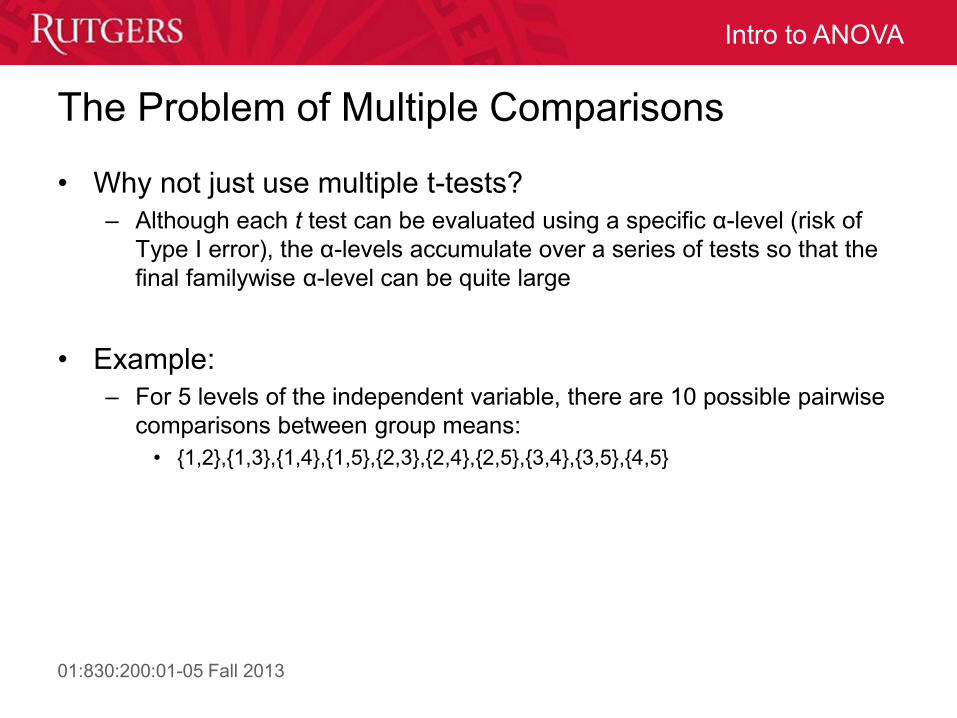
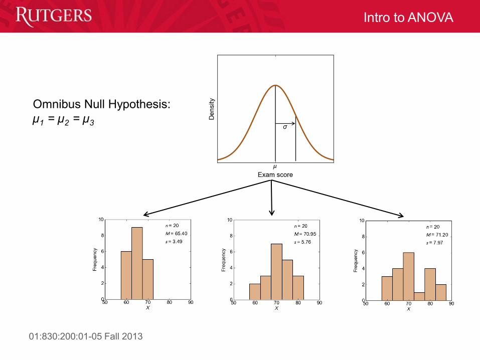
Null and Alternative Hypotheses in ANOVAs

• The omnibus null hypothesis is the null hypothesis in the

ANOVA: that the population means of all groups being

compared are equal

– i.e., for three groups, H0: μ1= μ2= μ3

• Alternative Hypothesis: at least one population mean is

different from the others.

01:830:200:01-05 Fall 2013

Intro to ANOVA

Omnibus Null Hypothesis:

µ1 = µ2 = µ3

01:830:200:01-05 Fall 2013

Intro to ANOVA

The Logic of the Analysis of Variance

• The test statistic for ANOVA is an F-ratio, which is a ratio of

two sample variances.

• In the context of ANOVA, the sample variances are called

mean squares, or MS values

– The numerator, MSbetween, measures the size of mean differences

between samples from different treatment groups

– The denominator, MSwithin (or MSerror), measures the magnitude of

differences that would be expected without any treatment effects

variance including any treatment effects

variance without any treatment effects

between

within

MSF

MS

01:830:200:01-05 Fall 2013

Intro to ANOVA

The Logic of the Analysis of Variance

Total Variance

Between

Treatments

Variance

Within

Treatments

Variance

Measures differences caused by:

• Systematic treatment effects

• Sampling error

Measures differences caused by:

• Sampling error

01:830:200:01-05 Fall 2013

Intro to ANOVA

Assumptions of the ANOVA

• Normality of Scores – I.e., we assume that the scores in all of our group populations are

normally distributed

– Since this is important primarily for the sampling distribution of the mean, the ANOVA is fairly robust to violations of this assumption, especially if the sample sizes are reasonably large

• Homogeneity of variances – We assume that each population of scores has the same variance

– E.g., [error variance]

– ANOVA is fairly robust to violations of this assumption

• Independence of observations – E.g., given the population parameters, knowing one person’s score tells

you nothing about another person’s score.

– Violations of this assumption can have serious implications for an analysis.

01:830:200:01-05 Fall 2013

Intro to ANOVA

The Logic of the ANOVA

• Regardless of whether or not the null hypothesis is true, the

assumption of homogeneity of variances implies that all

population variances are equal

• As we did in the independent-samples t-test, we can estimate

this shared population variance by taking the average of the

sample variances (the pooled variance)

1

2 2

2

2 2

3

2 32

2 2 22 2 2 2 2

31

1 , ,3

ˆwithi pn

s s ss Avg s s s

(assuming n1 = n2 = n3)

01:830:200:01-05 Fall 2013

Intro to ANOVA

The Logic of the ANOVA

• However, if all the population means are equal (under H0),

then we have a second way to estimate the population

variance

– we can estimate the population variance using the variance of the

sample means

• Recall that the Central Limit Theorem tells us how to compute

the variance of sample means from the population variance:

• We can rearrange this formula to solve for the population

variance given the variance of sample means:

22

Mn

2 2

Mn

01:830:200:01-05 Fall 2013

Intro to ANOVA

The Logic of the ANOVA

• Of course, we don’t have the variance of sample means

either. However, we can estimate it by computing the variance

of our three group means

• Plugging this into the previous equation, our second estimate

of the population variance is

1 2 3

2 2 , ,ˆM Ms Var M M M

2 2ˆbetween Mns

01:830:200:01-05 Fall 2013

Intro to ANOVA

The Logic of the ANOVA

We now have two estimates of the population variance:

• An estimate computed from the sample variances, which

should estimate the population variance regardless of whether

H0 is true

• A second estimate computed from the sample means, which

only estimates the population variance if H0 is true

2 3

2 2 2 2 2

1 , ,ˆwith n pi s Avg s s s

2 2

2 31ˆ , ,betwe Men ns nVar M M M

01:830:200:01-05 Fall 2013

Intro to ANOVA

The Logic of the ANOVA

• The F-ratio used as the test statistic for the ANOVA is simply the

ratio between these two estimates of the population variance

• If H0 is true, then these two estimates should be equal (on average)

– In this case, the ratio should be 1.0

• However, if H0 is false, then the estimate in the numerator (which is

based on the variability of sample means) will include the treatment

effect in addition to differences in sample means expected by

chance

– In this case, the ratio should be greater than 1.0

21

2

2 3

2 3

2 2 2

1

, ,

,

ˆ

ˆ ,

between

with

between

i inwith n

nVar M MMSF

MS A

M

vg s s s

01:830:200:01-05 Fall 2013

Intro to ANOVA

The F distribution

reject H0

accept H0

01:830:200:01-05 Fall 2013

Intro to ANOVA

Populations

Samples