T. Colak, R. Qahwaji, O. Ahmad, and P. Higgins - Space Weather

Automated Solar Flare Prediction: Is it a myth?

European Space Weather Week 7

15-19 November, 2010 - Brugge, Belgium

Tufan Colak,

[email protected]

Rami Qahwaji, Omar W. Ahmed, Paul Higgins*

University of Bradford , U.K. ,Trinity Collage Dublin, Ireland*

Space Weather Research Group

http://spaceweather.inf.brad.ac.uk/

Organisation of this talk:

Introduction

ASAP and SMART

SMART properties and Association with Solar

Flares

Solar Flare prediction results

Determining important SMART properties

Conclusions

European Space Weather Week 7, 15-19 November, 2010

Brugge, Belgium

Space Weather Research Group http://spaceweather.inf.brad.ac.uk/

T. Colak





Brugge, Belgium


T. Colak

Introduction• Space Weather is started getting more attention from public due to increased media

coverage, new solar cycle, movies (e.g. Knowing), global warming and Mayan Calendar .

• Last week, the Science and Technology Committee in U.K. takes evidence on the Government's

ability to deal with space weather events in a session on scientific advice and evidence in

emergencies. (Prof. Mike Hapgood (Royal Astronomical Society), Prof. Paul Cannon (Royal

Academy of Engineering), Chris Train (Network Operations Director, National Grid))

http://tinyurl.com/2v3e9qw.

• It is important to be able to detect, predict or forecast solar activities because it is

challenging.

• In this work I am going to talk about our on going solar flare prediction efforts in University of

Bradford.




http://tinyurl.com/2v3e9qw












Brugge, Belgium


T. Colak

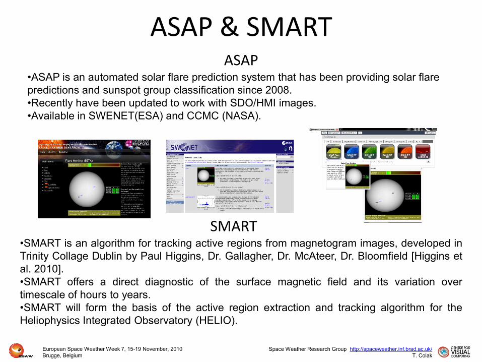
ASAP & SMART

•SMART is an algorithm for tracking active regions from magnetogram images, developed in

Trinity Collage Dublin by Paul Higgins, Dr. Gallagher, Dr. McAteer, Dr. Bloomfield [Higgins et

al. 2010].

•SMART offers a direct diagnostic of the surface magnetic field and its variation over

timescale of hours to years.

•SMART will form the basis of the active region extraction and tracking algorithm for the

Heliophysics Integrated Observatory (HELIO).

SMART

ASAP•ASAP is an automated solar flare prediction system that has been providing solar flare

predictions and sunspot group classification since 2008.

•Recently have been updated to work with SDO/HMI images.

•Available in SWENET(ESA) and CCMC (NASA).




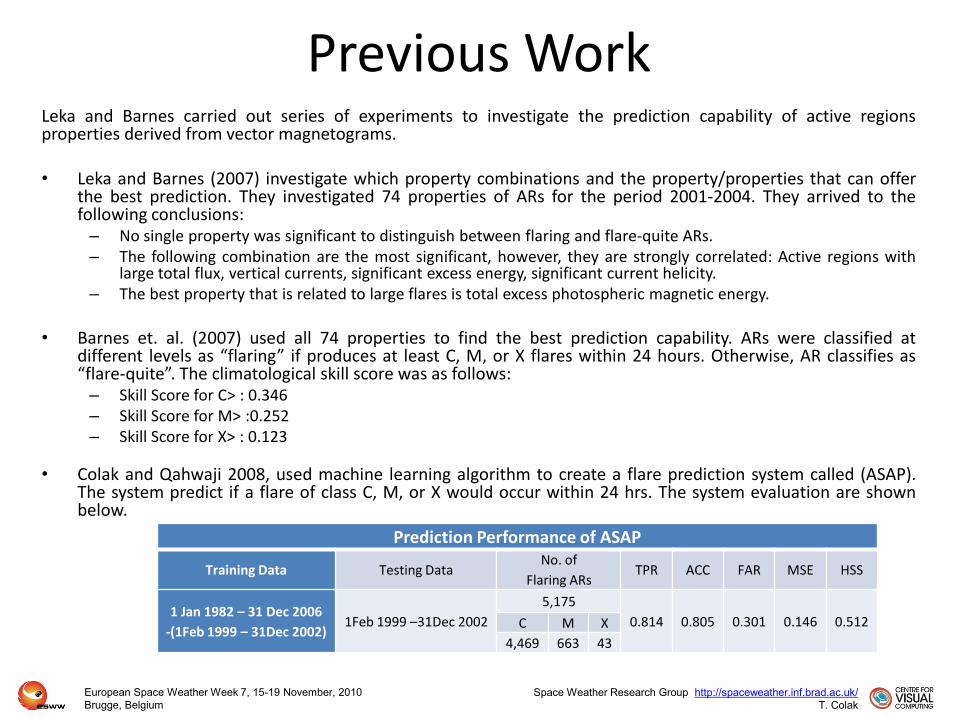
Previous WorkLeka and Barnes carried out series of experiments to investigate the prediction capability of active regionsproperties derived from vector magnetograms.

• Leka and Barnes (2007) investigate which property combinations and the property/properties that can offerthe best prediction. They investigated 74 properties of ARs for the period 2001-2004. They arrived to thefollowing conclusions:– No single property was significant to distinguish between flaring and flare-quite ARs.– The following combination are the most significant, however, they are strongly correlated: Active regions with

large total flux, vertical currents, significant excess energy, significant current helicity.– The best property that is related to large flares is total excess photospheric magnetic energy.

• Barnes et. al. (2007) used all 74 properties to find the best prediction capability. ARs were classified atdifferent levels as “flaring” if produces at least C, M, or X flares within 24 hours. Otherwise, AR classifies as“flare-quite”. The climatological skill score was as follows:– Skill Score for C> : 0.346– Skill Score for M> :0.252– Skill Score for X> : 0.123

• Colak and Qahwaji 2008, used machine learning algorithm to create a flare prediction system called (ASAP).The system predict if a flare of class C, M, or X would occur within 24 hrs. The system evaluation are shownbelow.

Prediction Performance of ASAP

Training Data Testing DataNo. of

Flaring ARsTPR ACC FAR MSE HSS

1 Jan 1982 – 31 Dec 2006

-(1Feb 1999 – 31Dec 2002)1Feb 1999 –31Dec 2002

5,175

0.814 0.805 0.301 0.146 0.512C M X

4,469 663 43


Brugge, Belgium


T. Colak




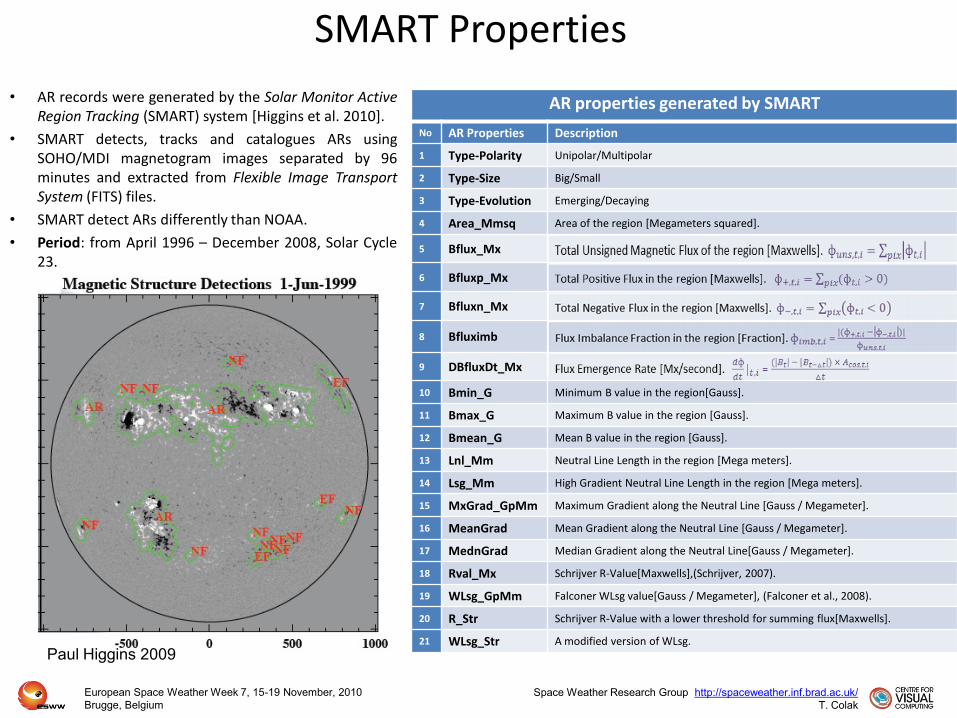
SMART Properties

AR properties generated by SMART

No AR Properties Description

1 Type-Polarity Unipolar/Multipolar

2 Type-Size Big/Small

3 Type-Evolution Emerging/Decaying

4 Area_Mmsq Area of the region [Megameters squared].

5 Bflux_Mx

6 Bfluxp_Mx

7 Bfluxn_Mx

8 Bfluximb

9 DBfluxDt_Mx

10 Bmin_G Minimum B value in the region[Gauss].

11 Bmax_G Maximum B value in the region [Gauss].

12 Bmean_G Mean B value in the region [Gauss].

13 Lnl_Mm Neutral Line Length in the region [Mega meters].

14 Lsg_Mm High Gradient Neutral Line Length in the region [Mega meters].

15 MxGrad_GpMm Maximum Gradient along the Neutral Line [Gauss / Megameter].

16 MeanGrad Mean Gradient along the Neutral Line [Gauss / Megameter].

17 MednGrad Median Gradient along the Neutral Line[Gauss / Megameter].

18 Rval_Mx Schrijver R-Value[Maxwells],(Schrijver, 2007).

19 WLsg_GpMm Falconer WLsg value[Gauss / Megameter], (Falconer et al., 2008).

20 R_Str Schrijver R-Value with a lower threshold for summing flux[Maxwells].

21 WLsg_Str A modified version of WLsg.

• AR records were generated by the Solar Monitor ActiveRegion Tracking (SMART) system [Higgins et al. 2010].

• SMART detects, tracks and catalogues ARs usingSOHO/MDI magnetogram images separated by 96minutes and extracted from Flexible Image TransportSystem (FITS) files.

• SMART detect ARs differently than NOAA.

• Period: from April 1996 – December 2008, Solar Cycle23.

Paul Higgins 2009


Brugge, Belgium


T. Colak




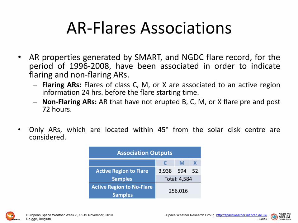
AR-Flares Associations

• AR properties generated by SMART, and NGDC flare record, for theperiod of 1996-2008, have been associated in order to indicateflaring and non-flaring ARs.– Flaring ARs: Flares of class C, M, or X are associated to an active region

information 24 hrs. before the flare starting time.– Non-Flaring ARs: AR that have not erupted B, C, M, or X flare pre and post

72 hours.

• Only ARs, which are located within 45° from the solar disk centre areconsidered.

Association Outputs

C M X

Active Region to Flare

Samples

3,938 594 52

Total: 4,584

Active Region to No-Flare

Samples256,016


Brugge, Belgium


T. Colak




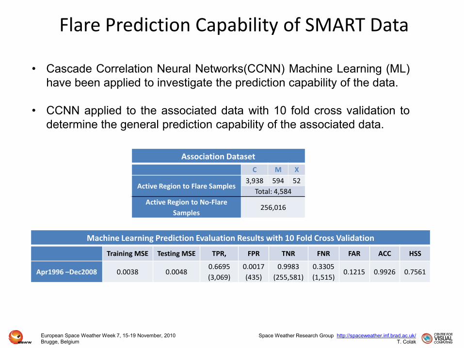
Flare Prediction Capability of SMART Data

Machine Learning Prediction Evaluation Results with 10 Fold Cross Validation

Training MSE Testing MSE TPR, FPR TNR FNR FAR ACC HSS

Apr1996 –Dec2008 0.0038 0.00480.6695

(3,069)

0.0017

(435)

0.9983

(255,581)

0.3305

(1,515)0.1215 0.9926 0.7561

Association Dataset

C M X

Active Region to Flare Samples3,938 594 52

Total: 4,584

Active Region to No-Flare

Samples256,016

• Cascade Correlation Neural Networks(CCNN) Machine Learning (ML)

have been applied to investigate the prediction capability of the data.

• CCNN applied to the associated data with 10 fold cross validation to

determine the general prediction capability of the associated data.


Brugge, Belgium


T. Colak




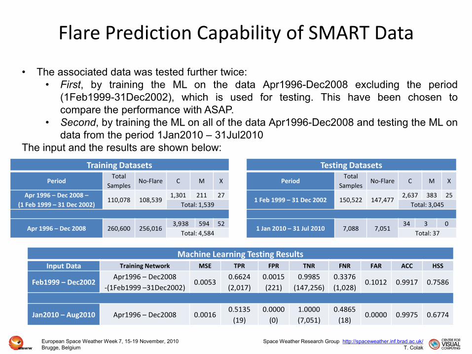
Flare Prediction Capability of SMART Data

Training Datasets

PeriodTotal

SamplesNo-Flare C M X

Apr 1996 – Dec 2008 –

(1 Feb 1999 – 31 Dec 2002)110,078 108,539

1,301 211 27

Total: 1,539

Apr 1996 – Dec 2008 260,600 256,0163,938 594 52

Total: 4,584

Testing Datasets

PeriodTotal

SamplesNo-Flare C M X

1 Feb 1999 – 31 Dec 2002 150,522 147,4772,637 383 25

Total: 3,045

1 Jan 2010 – 31 Jul 2010 7,088 7,05134 3 0

Total: 37

Machine Learning Testing ResultsInput Data Training Network MSE TPR FPR TNR FNR FAR ACC HSS

Feb1999 – Dec2002Apr1996 – Dec2008

-(1Feb1999 –31Dec2002)0.0053

0.6624

(2,017)

0.0015

(221)

0.9985

(147,256)

0.3376

(1,028)0.1012 0.9917 0.7586

Jan2010 – Aug2010 Apr1996 – Dec2008 0.00160.5135

(19)

0.0000

(0)

1.0000

(7,051)

0.4865

(18)0.0000 0.9975 0.6774

• The associated data was tested further twice:

• First, by training the ML on the data Apr1996-Dec2008 excluding the period

(1Feb1999-31Dec2002), which is used for testing. This have been chosen to

compare the performance with ASAP.

• Second, by training the ML on all of the data Apr1996-Dec2008 and testing the ML on

data from the period 1Jan2010 – 31Jul2010

The input and the results are shown below:


Brugge, Belgium


T. Colak




Correlation Coefficient between the Properties as well as the Class

v1 v2 v3 v4 v5 v6 v7 v8 v9 v10 v11 v12 v13 v14 v15 v16 v17 v18 v19 v20 v21 Class

v1 1.000 0.391 -0.007 0.429 0.316 0.248 0.311 -0.898 -0.004 -0.614 0.593 -0.010 0.291 0.216 0.552 0.631 0.618 0.144 0.187 0.178 0.240 0.209 v1

v2 0.391 1.000 -0.005 0.401 0.243 0.196 0.232 -0.415 0.000 -0.380 0.380 0.007 0.155 0.117 0.282 0.308 0.296 0.078 0.101 0.096 0.129 0.114 v2

v3 -0.007 -0.005 1.000 -0.005 -0.003 0.000 -0.006 0.006 0.012 0.002 -0.010 -0.009 -0.007 -0.008 -0.009 -0.008 -0.007 -0.006 -0.008 -0.005 -0.008 -0.003 v3

v4 0.429 0.401 -0.005 1.000 0.798 0.637 0.771 -0.491 0.002 -0.558 0.555 -0.003 0.672 0.574 0.605 0.461 0.392 0.509 0.518 0.591 0.604 0.543 v4

v5 0.316 0.243 -0.003 0.798 1.000 0.896 0.849 -0.375 0.226 -0.479 0.494 0.106 0.752 0.686 0.589 0.412 0.339 0.633 0.631 0.700 0.705 0.577 v5

v6 0.248 0.196 0.000 0.637 0.896 1.000 0.527 -0.295 0.585 -0.320 0.457 0.317 0.591 0.540 0.462 0.322 0.265 0.499 0.496 0.551 0.554 0.457 v6

v7 0.311 0.232 -0.006 0.771 0.849 0.527 1.000 -0.367 -0.263 -0.537 0.402 -0.174 0.737 0.672 0.579 0.406 0.335 0.618 0.619 0.684 0.691 0.561 v7

v8 -0.898 -0.415 0.006 -0.491 -0.375 -0.295 -0.367 1.000 0.004 0.658 -0.629 0.012 -0.345 -0.262 -0.582 -0.626 -0.600 -0.182 -0.226 -0.223 -0.287 -0.253 v8

v9 -0.004 0.000 0.012 0.002 0.226 0.585 -0.263 0.004 1.000 0.013 0.023 0.301 -0.004 -0.005 -0.004 -0.004 -0.004 -0.004 -0.006 -0.003 -0.005 -0.003 v9

v10 -0.614 -0.380 0.002 -0.558 -0.479 -0.320 -0.537 0.658 0.013 1.000 -0.343 0.411 -0.491 -0.400 -0.664 -0.618 -0.561 -0.306 -0.359 -0.360 -0.433 -0.377 v10

v11 0.593 0.380 -0.010 0.555 0.494 0.457 0.402 -0.629 0.023 -0.343 1.000 0.427 0.487 0.401 0.630 0.579 0.522 0.310 0.356 0.363 0.427 0.381 v11

v12 -0.010 0.007 -0.009 -0.003 0.106 0.317 -0.174 0.012 0.301 0.411 0.427 1.000 -0.013 -0.011 -0.017 -0.015 -0.013 -0.008 -0.011 -0.009 -0.013 -0.006 v12

v13 0.291 0.155 -0.007 0.672 0.752 0.591 0.737 -0.345 -0.004 -0.491 0.487 -0.013 1.000 0.942 0.714 0.462 0.368 0.872 0.883 0.938 0.962 0.715 v13

v14 0.216 0.117 -0.008 0.574 0.686 0.540 0.672 -0.262 -0.005 -0.400 0.401 -0.011 0.942 1.000 0.647 0.412 0.327 0.944 0.975 0.932 0.984 0.661 v14

v15 0.552 0.282 -0.009 0.605 0.589 0.462 0.579 -0.582 -0.004 -0.664 0.630 -0.017 0.714 0.647 1.000 0.882 0.782 0.508 0.617 0.556 0.689 0.563 v15

v16 0.631 0.308 -0.008 0.461 0.412 0.322 0.406 -0.626 -0.004 -0.618 0.579 -0.015 0.462 0.412 0.882 1.000 0.966 0.289 0.387 0.319 0.446 0.355 v16

v17 0.618 0.296 -0.007 0.392 0.339 0.265 0.335 -0.600 -0.004 -0.561 0.522 -0.013 0.368 0.327 0.782 0.966 1.000 0.221 0.304 0.245 0.355 0.276 v17

v18 0.144 0.078 -0.006 0.509 0.633 0.499 0.618 -0.182 -0.004 -0.306 0.310 -0.008 0.872 0.944 0.508 0.289 0.221 1.000 0.935 0.965 0.929 0.561 v18

v19 0.187 0.101 -0.008 0.518 0.631 0.496 0.619 -0.226 -0.006 -0.359 0.356 -0.011 0.883 0.975 0.617 0.387 0.304 0.935 1.000 0.889 0.973 0.606 v19

v20 0.178 0.096 -0.005 0.591 0.700 0.551 0.684 -0.223 -0.003 -0.360 0.363 -0.009 0.938 0.932 0.556 0.319 0.245 0.965 0.889 1.000 0.937 0.630 v20

v21 0.240 0.129 -0.008 0.604 0.705 0.554 0.691 -0.287 -0.005 -0.433 0.427 -0.013 0.962 0.984 0.689 0.446 0.355 0.929 0.973 0.937 1.000 0.678 v21

Class 0.209 0.114 -0.003 0.543 0.577 0.457 0.561 -0.253 -0.003 -0.377 0.381 -0.006 0.715 0.661 0.563 0.355 0.276 0.561 0.606 0.630 0.678 1.000 Class

v1 v2 v3 v4 v5 v6 v7 v8 v9 v10 v11 v12 v13 v14 v15 v16 v17 v18 v19 v20 v21 Class

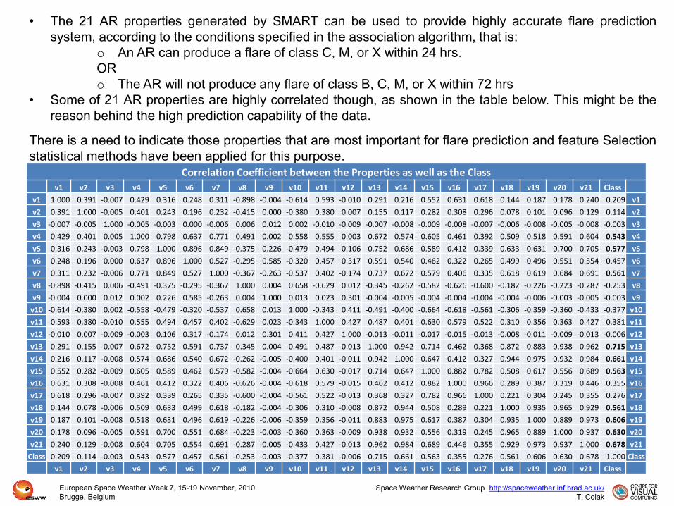
• The 21 AR properties generated by SMART can be used to provide highly accurate flare prediction

system, according to the conditions specified in the association algorithm, that is:

o An AR can produce a flare of class C, M, or X within 24 hrs.

OR

o The AR will not produce any flare of class B, C, M, or X within 72 hrs

• Some of 21 AR properties are highly correlated though, as shown in the table below. This might be the

reason behind the high prediction capability of the data.

There is a need to indicate those properties that are most important for flare prediction and feature Selection

statistical methods have been applied for this purpose.


Brugge, Belgium


T. Colak




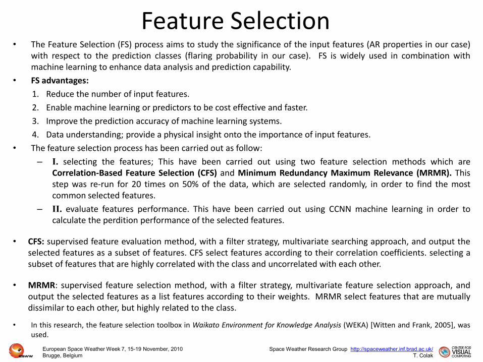
Feature Selection• The Feature Selection (FS) process aims to study the significance of the input features (AR properties in our case)

with respect to the prediction classes (flaring probability in our case). FS is widely used in combination withmachine learning to enhance data analysis and prediction capability.

• FS advantages:

1. Reduce the number of input features.

2. Enable machine learning or predictors to be cost effective and faster.

3. Improve the prediction accuracy of machine learning systems.

4. Data understanding; provide a physical insight onto the importance of input features.

• The feature selection process has been carried out as follow:

– I. selecting the features; This have been carried out using two feature selection methods which areCorrelation-Based Feature Selection (CFS) and Minimum Redundancy Maximum Relevance (MRMR). Thisstep was re-run for 20 times on 50% of the data, which are selected randomly, in order to find the mostcommon selected features.

– II. evaluate features performance. This have been carried out using CCNN machine learning in order tocalculate the perdition performance of the selected features.

• CFS: supervised feature evaluation method, with a filter strategy, multivariate searching approach, and output theselected features as a subset of features. CFS select features according to their correlation coefficients. selecting asubset of features that are highly correlated with the class and uncorrelated with each other.

• MRMR: supervised feature selection method, with a filter strategy, multivariate feature selection approach, andoutput the selected features as a list features according to their weights. MRMR select features that are mutuallydissimilar to each other, but highly related to the class.

• In this research, the feature selection toolbox in Waikato Environment for Knowledge Analysis (WEKA) [Witten and Frank, 2005], wasused.


Brugge, Belgium


T. Colak




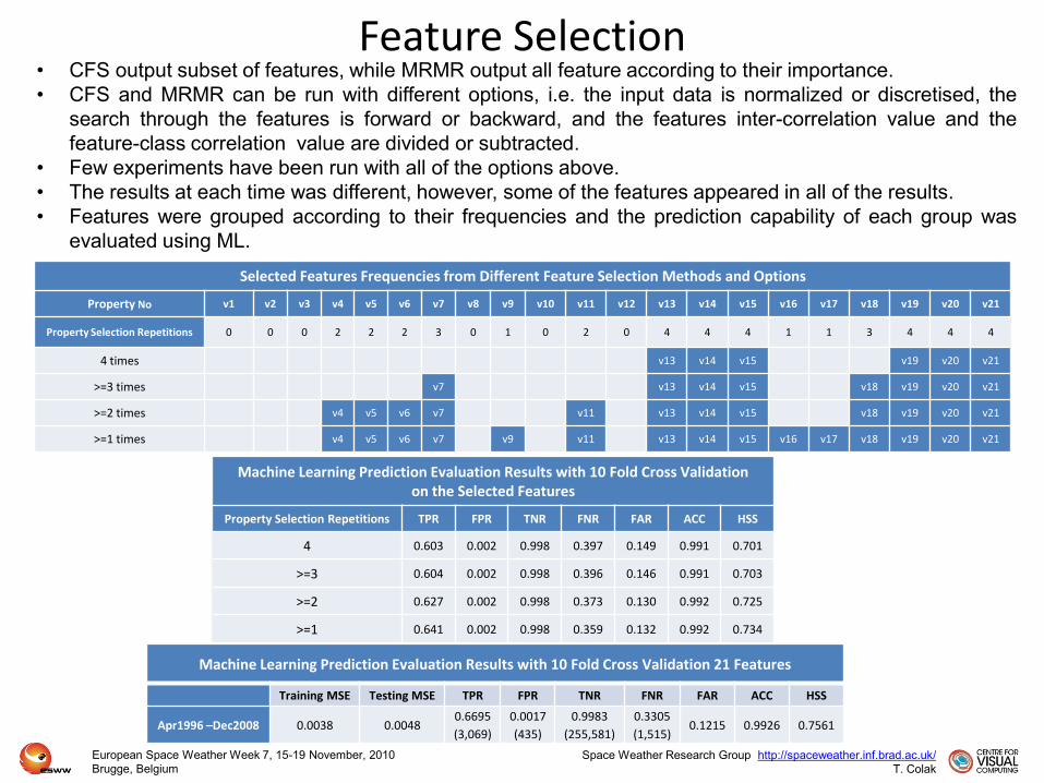
Feature Selection

Selected Features Frequencies from Different Feature Selection Methods and Options

Property No v1 v2 v3 v4 v5 v6 v7 v8 v9 v10 v11 v12 v13 v14 v15 v16 v17 v18 v19 v20 v21

Property Selection Repetitions 0 0 0 2 2 2 3 0 1 0 2 0 4 4 4 1 1 3 4 4 4

4 times v13 v14 v15 v19 v20 v21

>=3 times v7 v13 v14 v15 v18 v19 v20 v21

>=2 times v4 v5 v6 v7 v11 v13 v14 v15 v18 v19 v20 v21

>=1 times v4 v5 v6 v7 v9 v11 v13 v14 v15 v16 v17 v18 v19 v20 v21

Machine Learning Prediction Evaluation Results with 10 Fold Cross Validation 21 Features

Training MSE Testing MSE TPR FPR TNR FNR FAR ACC HSS

Apr1996 –Dec2008 0.0038 0.00480.6695

(3,069)

0.0017

(435)

0.9983

(255,581)

0.3305

(1,515)0.1215 0.9926 0.7561

• CFS output subset of features, while MRMR output all feature according to their importance.

• CFS and MRMR can be run with different options, i.e. the input data is normalized or discretised, the

search through the features is forward or backward, and the features inter-correlation value and the

feature-class correlation value are divided or subtracted.

• Few experiments have been run with all of the options above.

• The results at each time was different, however, some of the features appeared in all of the results.

• Features were grouped according to their frequencies and the prediction capability of each group was

evaluated using ML.

Machine Learning Prediction Evaluation Results with 10 Fold Cross Validationon the Selected Features

Property Selection Repetitions TPR FPR TNR FNR FAR ACC HSS

4 0.603 0.002 0.998 0.397 0.149 0.991 0.701

>=3 0.604 0.002 0.998 0.396 0.146 0.991 0.703

>=2 0.627 0.002 0.998 0.373 0.130 0.992 0.725

>=1 0.641 0.002 0.998 0.359 0.132 0.992 0.734


Brugge, Belgium


T. Colak





Brugge, Belgium


T. Colak

Conclusions

• Automated Solar Flare Prediction is a myth?? NO

• Properties extracted by SMART can be used to predict solar flares better than currently

online ASAP.

• Certain SMART properties related to neutral lines such as : Neutral line length , high

gradient neutral line length, maximum gradient along the neutral line length are important

indicators of flaring or non-flaring.

• SMART properties related to area and total flux are important discriminators for solar flares.

• Also Schrijver R-value and Falconer WLsg values are important properties.

• In the future these properties might be combined with ASAP to provide better solar flare

prediction results. (Possible name: SMART ASAP)




Documents

T. Colak, R. Qahwaji, O. Ahmad, and P. Higgins - Space Weather