Embed Size (px)
Citation preview

A R a I ij
- —
Semi-leptonic Decays
on the Lattice
Nicholas Mark Hazel
a
:!..! 7Fh6" ,-T-, r 7,A V
Doctor of Philosophy
The University of Edinburgh
1996

To Mum and Dad.

Abstract
This thesis describes a lattice calculation of the matrix elements of the vector
and axial-vector currents which are relevant to the semi-leptonic decays D -p K
and D -+ K* . The simulation was performed in the quenched approximation to
lattice QCD on a 24 x 48 space-time lattice at 0 = 6.2, using an 0(a)-improved
fermionic action. In the limit of zero lepton masses the D -* K and D -* K*
decays are described by four form factors: f, VK*, and A. which are
dimensionless functions of q2 , where q 11 is the four-momentum transfer. The main
results, for the form factors at q2 = 0, are as follows:
f(0) = 0 . 67+ 005 + 0 .03 - 0.03 - 0.04
VK.(0) = 1.01+0.25+0.05 - 0.05 - 0.06
Ak-s (0) = 0.69 + 0.06+0.01 - 0.03- 0.05
A<.(0) = 063+ 0 . 12 + 0 .01 - 0.12 - 0.05
where the first set of errors are statistical and the second are an estimate of the
systematic error. These results are in good agreement with experiment. The
form factors were determined for different q2 values; their q2 dependence is found
to be reasonably well described by a simple pole-dominance model. The form
factors corresponding to the semi-leptonic decays D - rr and D - p were also
computed.
11

Declaration
This thesis has been composed wholly by me and contains my own work carried
out as a member of the UKQCD Collaboration. The analysis described in Chap-
ter 3 was performed under the initial guidance of Dave Richards and in the later
stages in collaboration with Juan Nieves in preparation for publication. The basic
routines for statistical analysis were written in conjunction with Henning Hoeber,
David Henty and Hugh Shanahan.
The results in Chapter 2 are compatible with values published in
C.R. Ailton et. at. (UKQCD Collaboration), Phys. Rev. D49 (1994) 474.
. R.M. Baxter et. at. (UKQCD Collaboration), Phys. Rev. D49 (1994) 1594.
and the results in Chapter 3 are published in
. K.C. Bowler et. at. (UKQCD Collaboration), Phys. Rev. D51 (1995) 4905.
Other related publications to which I have contributed include
. N.M. Hazel (UKQCD Collaboration), Nuci. Phys. B (Proc. Suppi.) 34
(1994) 471.
. S.P. Booth et. at. (UKQCD Collaboration), Phys. Rev. Lett. 72 (1994) 462.
• K.C. Bowler et. at. (UKQCD Collaboration), Phys. Rev. Lett. 72 (1994)
1398.
• K.C. Bowler et. at. (UIKQCD Collaboration), Phys. Rev. D51 (1995) 4955.
• K.C. Bowler et. at. (UKQCD Collaboration), Phys. Rev. D52 (1995) 5067.
• D.R.Burford et. at. (UKQCD Collaboration), Nuci. Phys. B447 (1995) 425.
• J.M. Flynn et. at. (UKQCD Collaboration), Nuci. Phys. B461 (1996) 327.
111

Acknowledgements
I dedicate this thesis to my family whose support and encouragement have made
it possible. I would also like to thank my supervisors Ken Bowler and Brian
Pendleton, and Professor Richard Kenway, for their guidance and support, and
for providing access to the funds to attend Lattice 93. Thanks to Dave Richards
and David Henty for useful discussions and suggestions during my research. I
also enjoyed collaborating with Juan Nieves from Southampton University in the
preparation of a UKQCD publication.
I had the pleasure to work alongside my fellow postgrads Henning Hoeber, Hugh
Shanahan, Nick Stanford and John Mehegan. I wish them all the best in their
future careers. I have also enjoyed sharing an office, and far too many coffee
breaks, with Harry Newton, Orlando Oliveira, Mike Peardon and Sinead Ryan. I
am particularly in debt to Harry and Mike for letting me stay at Montague Street
during my 'homeless' period.
During my stay in Edinburgh I spent two great years at 5 Roseneath St. with my
extended family Dave, James and Mark - the 'boyz from the flat'. These 'guys'
provided me with an escape from the social isolation of the physics department
and an appallingly bad taste in music. Good luck with your respective careers in
Medicine (x2) and Veterinary Practice. More recently, I have enjoyed sharing a
flat with Pete Evans, Chris Jowett and David Parratt.
I have had the good fortune to know Adam Davis, Graham Ford and Charlie Tripp
with whom I have shared the more memorable experiences in my life. Thanks for
the epic expeditions, wild drinking escapades and disturbing philosophical debates.
Finally I acknowledge the financial support of the Particle Physics and Astronomy
Research Council, and my personal sponsors Mr. Access and Mr. Visa.
IV

Henry IV, Part 1
(Close of Act 1, Scene 2)
Prince Henry
I know you all, and will awhile uphold
The unyoked humour of your idleness:
Yet herein will I imitate the sun,
Who doth permit the base contagious clouds
To smother up his beauty from the world,
That, when he please again to be himself,
Begin wanted, he may be more wonder'd at,
By breaking through the fowl and ugly mists
Of vapours that did seem to strangle him.
If all the year were playing holidays,
To sport would be as tedious as to work;
But when they seldom come, they wish'd for come,
And nothing pleaseth but rare accidents.
So, when this loose behavior I throw off
And pay the debt I never promised,
By how much better than my word I am,
By so much shall I falsify men's hopes;
And like bright metal on a sullen ground,
My reformation, glittering o'er my fault,
Shall show more goodly and attract more eyes
Than that which hath no foil to set it off.
I'll so offend, to make offence a skill;
Redeeming time when men think least I will.
[Exit]
William Shakespeare

Contents
Abstract ii
Declaration iii
Acknowledgements iv
Introduction 1
1 Lattice QCD 5
1.1 QCD 5
1.2 Lattice QCD 9
1.3 Improved Actions 17
1.4 Lattice Simulations 20
1.5 Two-Point Functions 22
1.6 Meson Masses 25
1.7 Three-Point Functions 28
1.8 Weak Matrix Elements 31
2 Meson Spectrum 34
2.1 Simulation Details 34
2.2 Statistical Analysis 35
2.3 Two-Point Correlator Fits 38
2.4 Chiral Extrapolation 46
2.5 Physical Meson Spectrum 52
3 Semi-Leptonic D Decays 55
3.1 Phenomenology 55
3.2 Experimental Results 59
3.3 Three-Point Correlator Fits 61
3.4 Form Factor Extrapolations 80
3.5 Pole Dominance Fits 88
3.6 Renormalisation Constants 100
3.7 Comparison with Experiment 103
Conclusions 112

References
113
vi"

Introduction
The Standard Model (SM) of Particle Physics [1, 2, 3] describes the interaction
of the elementary particles, the quarks and leptons, in terms of the strong, weak
and electromagnetic forces. These forces are mediated by gauge bosons: the
gluon, Wii and Z, and the photon respectively. This model has been successful
in explaining many of the observed experimental phenomena, over a wide range
of energies. However, the SM has some unsatisfactory features: the large number
of free parameters (> 20) required as input, and no quantum theory of gravity.
Tests of the SM have focused on determining these free parameters in a search for
new physics.
Many parameters in the weak sector of the SM are under-determined. The
Cabibbo-Kobayashi-Maskawa (CKM) matrix elements describe how the quarks
participate in the weak interaction. However, only the weak decays of mesons
and baryons are observed experimentally; the strong force confines quarks within
hadrons. Unfortunately, the relevant weak processes occur at low energies where
the quark-gluon coupling is of 0(1). Thus, perturbation theory fails and one must
rely on non-perturbative approaches, such as quark models and QCD sum rules,
in order to extract information on the CKM matrix elements from experimental
measurements. On the lattice, the non-perturbative quark-gluon contribution can
be computed from first principles.
The semi-leptonic decays of heavy-light mesons provide a window on the CKM
matrix elements; the square of the relevant CKM matrix element appears as an
overall factor in the decay rate. These decays proceed via the spectator process
whereby the heavy quark decays into a 'lighter' quark by emitting a W boson
(which decays into a lepton pair); the common light quark plays no part in the
interaction. Figure 0.1 shows the Feynman diagram relevant in semi-leptonic
D -+ K, K* decays. Semi-leptonic decays are particularly simple since there is a
single hadron only in the final state. Thus, there are no interference diagrams or
final state interactions to take into account, unlike the case of non-leptonic decays.
1

VI
1<1+
U
Figure 0.1: Feynman diagram relevant in semi-leptonic D —4 K, K* decays.
Charged Weak Currents
The SM Lagrangian describing the charged-current interaction is given by
= (J + J(L) W+ + h.c. (0.1)
d\
j= (u, )(1—)V cKM ( 1 (0.2)
b)
/ e\
= (De,Flo, 0)(1 _5) I (0.3)
where J and J[L are the hadronic and leptonic vector-minus-axial-vector (V-A)
currents respectively which couple to the massive gauge vector bosons, W±, and
9 is the SU(2) gauge coupling constant.
with
and

3
The CKM matrix [4, 5] is given by
'Vud V.s Vb\
VCKM = Vcd Vcs Vcb (0.4)
Vtd Vts Vtb)
where VCKM is a 3 x 3 unitary matrix which can be parameterised by three real
angles and one complex phase. The CKM matrix arises in the SM through the
Higgs mechanism [6] which generates mass terms for both the fermions and the
gauge vector bosons, W and Z, in a renormalisable way.
For momentum transfer much less than the vector gauge boson mass (mw
80 GeV) an effective Lagrangian can be constructed as follows:
Leff- CF jt j (0.5) cc - -
with GF_ g2
(0.6) V12 8m
which corresponds to the low-energy V-A theory [7, 8, 9].
Weak Matrix Elements
Consider the semi-leptonic decay D —+ K 1+v, the transition amplitude is defined
as follows:
T = (K1+v I Hejj (0.7)
with GF
Heff -
_ijfJIL (0.8)
where Heff is the effective weak Hamiltonian. Factorising the leptonic and hadronic
currents in Eqn. (0.7) gives
T=IV3ILH (0.9)
with
U

4
= fi(1)y,L (l —'y 5 )u(u) (0.10)
= (K-y(1—y 5 )sD) (0.11)
where v and u are Dirac spinors and H is the weak matrix element required to
extract the CKM matrix element IV,,l from the decay rate; the leptonic matrix
element L follows from tree-level perturbation theory. Clearly, H includes non-
perturbative strong interaction effects. On the lattice this matrix element can be
computed from first principles.
In recent years, a machinery has been developed for calculating weak matrix
elements on the lattice [10]—[15]. The lattice is the only non-perturbative method
for computing strong interaction effects which is systematically improvable. For
lattice methods to gain acceptance as a useful phenomenological tool it is essential
to show that systematic errors are under control. The study of D decays provides
an important test of the lattice method since the relevant CKM matrix elements
are well-constrained in the SM by three-generation unitarity. Furthermore, such
tests give us confidence in our predictions for B decays [16]—[21] where the relevant
CKM matrix elements are under-determined.
Overview
Chapter 1 begins with a brief introduction to Quantum Chromodynamics, the
gauge theory which describes the strong interaction. The lattice gauge formula-
tion is then described; this is motivated by a simple geometric interpretation of the
gauge principle. Finally, the lattice machinery required to construct weak matrix
elements is presented. Chapter 2 presents a lattice calculation of the light-light and
heavy-light meson spectrum. These masses and the corresponding two-point am-
plitudes are required to extract the form factors which describe the semi-leptonic
decays. Chapter 3 describes a lattice calculation of the matrix elements of the
vector and axial-vector currents which are relevant for the semi-leptonic decays
D -+ K and D -+ K* . The form factors describing these decays are determined
and their q2 dependence investigated, where q 11 is the four-momentum transfer.
The decay rates are also computed. Finally, these results are compared with
experiment and other theoretical calculations.

Chapter 1
Lattice QCD
This chapter describes the lattice formulation of QCD. At low energies QCD is
non:perturbative; it is this non-perturbative nature which is expected to account
for the binding of quarks into hadrons. The lattice formulation [22]-[25] provides
a systematic first-principles approach to solving QCD.
1.1 QCD
Quantum Chromodynamics (QCD) is the theory of hadronic physics in which
quarks interact via the exchange of gluons [26]—[28]. The early quark model (con-
sisting of fractionally charged, spin-half particles) was successful in accounting for
many of the observed symmetries in the hadron spectrum. Problems with this
model (such as unobserved states) were resolved by postulating that the quarks
possess a 'hidden' degree of freedom, called colour.
Each quark flavour is assumed to occur in three colours which form a triplet
under a colour SU(3) group. Since colour is a hidden quantity only singlet states
are physically observable; and thus quarks cannot be free and must be confined
within hadrons. The allowed qq and qqq states reproduce the physical spectrum
of mesons and baryons respectively.
In deep inelastic scattering experiments, the hadronic constituents (the quarks)
behave at short distances as if only weakly bound. Thus phenomenologically, a
theory is required which exhibits both asymptotic freedom (the quark coupling
decreases at short distance) and quark confinement. The fact that only non-
abelian gauge theories are both asymptotically free and renormalisable [29, 30]
leads us to QCD.
5

Chapter 1. Lattice QCD
QCD Derived
QCD can be 'derived' by demanding that the Lagrangian density for a free quark
colour triplet 1' (of four-component Dirac spinors)
= (x)(i'ya - m)b(x)
(1.1)
be invariant under a local SU(3) symmetry transformation in which
(x) - (1.2)
(x) - '(x) = (x) U(0) 1
(1.3)
with
U(0) = exp (_iA.O(x))
(1.4)
where Aaand Oa(x) (a = 1, 2,. . . , 8) are the generators and group parameters
of SU(3) respectively. The Aas are the Cell-Mann matrices which satisfy the
following commutation relation and normalisation condition:
FAaAbl Ac b
L' = fa5c , Tr (AaA) = 28ab
(1.5)
The derivative term in Eqn. (1.1) spoils gauge invariance. By introducing vec-
tor gauge fields A(x) (one gauge gluon for each generator) a gauge invariant
derivative can be constructed through the minimal coupling as follows:
(1.6)
where g is the gauge coupling constant. D(x) must transform like '(x) which
implies the following symmetry transformation:
AA AA =U(0)(A 2 2
2 ) U(0)_ I - a[u(o)] U(0) 1 . ( 1.7)
Finally, a term involving the derivatives of the gauge fields is required to make the
gluon a truly dynamical variable. The simplest gauge invariant, renormalisable

Chapter 1. Lattice QCD
term (of dimension four or less) is
with
F' - 3A' II - aVA a+ gfabcAb A. (1.9)
Eqn. (1.8) contains terms which correspond to both trilinear and quadrilinear
couplings of the gauge fields, This self-coupling arises from the non-abelian
nature of the theory in which gluons, like quarks, carry colour-charge.
Thus, the QCD Lagrangian can be written as follows:
ml
£QCD = q (iD - Mk) qk -
k=1
where flj is the number of quark flavours. To satisfy phenomenological require-
ments, a theory of the strong interaction must exhibit both asymptotic freedom
and quark confinement. QCD is asymptotically free 'by design', and it can be
shown [25] (in the absence of vacuum polarisation effects) that the inter-quark
potential does indeed rise linearly with increasing separation. However, these
regimes may be separated by one or more discontinuous phase transitions. Thus,
further numerical investigation is required to determine whether QCD allows these
two necessary phenomena to coexist in a single phase.
QCD and Geometry
Like all gauge theories, QCD has a deep geometrical foundation. In this section,
following Cheng and Li [2], the basic geometrical concepts required to construct
a lattice gauge theory are introduced. A more complete description of the gauge
principle, using the language of differential geometry, can be found in Ref. [31].
Consider two vectors which are free to move on the circumference of a circle while
being held at some fixed angle to their tangent vectors. The relative 'orientation'
of these vectors is dependent on their position. In a curved space, a method is
required for comparing vectors which is independent of their position; and thus
uniquely defined.
7
(1.8)

Chapter 1. Lattice QCD 8
In a region of curved space (where the derivative of the metric is non-vanishing),
a vector in moving from x -+ x + dx will experience a change in 'scale' (due to the
change in the measure). The covariant derivative takes this scale transformation
into account and is defined as follows:
b(x+dx)—['çb(x)+S'çb(x)] D(x) = dx's
where &,b(x) is the change in b(x) in moving from x -+ x + dx, in the ri-direction.
This change is directly proportional to the vector itself, to the distance trav-
elled, and to a mathematical construction called the 'connection' (a term involving
derivatives of the metric).
Comparing Eqn. (1.6) with the general form for a covariant derivative (above)
gives the following relation:
JOW = i9 ( A
2) (x) dx (1.12)
where the minimal coupling ig (A. A)/2 can be identified as the connection in
charge space. Thus, the gauge principle has a geometric description in terms of a
curved charge space.
A useful geometric concept is parallel transport: the 'rescaling' of a vector at
every point along a path. The infinitesimal parallel transport operator is defined
as follows:
P(x + dx, x) O(x) = '(x) + SO(x) (1.13)
and using Eqns. (1.12) is given by
P(x + dx, x) = [i + ig (A. A(x)) dx] (1.14)
where I is the identity operator. The infinitesimal parallel transport operator
preserves the 'orientation' of a vector, '(x), in moving from x -+ x + dx.

Chapter 1. Lattice QCD 9
For parallel transport over a finite interval Eqn. (1.14) is exponentiated to obtain
( i'A.A,(y)2
d} SU(3) (1.15) P(x ix) = exp g I.x
where the line integral is ordered along the path joining x and x'. Under parallel
transport '(x) picks up a path-dependent phase factor. Thus, for every path
there is a corresponding group element. The quantity '(x') P(x', x) x) is clearly
gauge invariant. From Eqns. (1.2) and (1.3) the parallel transport operator must
transform as follows:
P(x',x) P'(x',x) = U(x')P(x',x)U(x) 1 (1.16)
which can be shown, using Eqn. (1.14), to be consistent with the original trans-
formation law for the minimal coupling.
Another important geometrical concept is the 'curvature tensor'. A space has non-
zero curvature if a vector experiences a change under parallel transport around
a closed path. This change is directly proportional to the vector itself, to the
area bounded by the path, and to the curvature tensor. By considering parallel
transport around an infinitesimal rectangle
P0 = P(x, y; x, y + dy) P(x, y + dy; x + dx, y + dy) x
P(x + dx, y + dy; x + dx, y) P(x + dx, y; x, y) (1.17)
and using the following matrix identity
e A e B eA (A + B) + [A, B] + 0(A
3 )
it can be shown that
exp 2 )dxdY} Po =
{ ig (A.F,\
which suggests identifying () as the curvature tensor in charge space. From
Eqn. (1.16) it is clear that parallel transport around any closed path is a gauge
invariant operation.

Chapter 1. Lattice QCD
10
1.2 Lattice QCD
In the Feynman path integral formalism [32] of Quantum Field Theory (QFT), the
vacuum expectation value of a time-ordered product of field operators is defined
in Minkowski space-time as:
(0 1 = JD[O] (Xi) . . . (x) eiS[] (1.20)
with
S[] = Yx L(x) (1.21)
where the path integral, D[], is over all possible configurations of the field
, weighted by an action, S[O], which is expressed in terms of a Lagrangian
density £(x).
For the path integral to be well-defined, in infinite time and volume limits, it is
necessary to work in Euclidean space-time. Analytically continuing Eqn. (1.20)
to imaginary time gives
(01 [(_ix, . .. (—ix ° , xN)] 0) = JD[] (Xi) . . . (x) (1.22)
with D[] e[]
(1.23) Du[q] = z
and
Z = JD[ç] e SSj (1.24)
where the probability measure, D14qf], is now well-defined. The Euclidean path
integral is equivalent to a statistical mechanics ensemble average with a Boltzmann
factor of (e_) where Z is the partition function. This equivalence allows the
path integral to be computed using methods borrowed from statistical mechanics.
Lattice Field Theory
To study the long distance properties of QCD (a strong coupling regime), a
non-perturbative method of evaluating the path integral is required. The lattice

Chapter 1. Lattice QCD 11
approach is to replace the continuum of space-time by a regular hyper-cubic
lattice' with lattice spacing a. The integral over space-time is approximated by
id 4X -+ a 4 (1.25)
where the sum is over all lattice sites, labelled by a four-vector .
The discretisation of space-time introduces a natural cut-off on momenta which
are restricted to a domain bounded by it/a; wavelengths less than twice the lattice
spacing have no lattice representation. Furthermore, the introduction of periodic
boundary conditions quantises the allowed values of.momenta:
2ir 7Ei= L(nx,ny)nz) (1.26)
where n, n, and n are integers, and L is the spatial extent of the lattice. As with
any cut-off prescription, there is considerable freedom in the lattice formulation.
This allows the regulation of unwanted lattice artifacts by the addition of non-
continuum terms to the lattice action which vanish in the continuum limit.
The physics of any renormalisable field theory should be independent of the cut-off,
in this case the lattice spacing. In this regime, the correlation length of the theory
should be infinite compared to the lattice spacing. In statistical mechanics, this
is achieved by tuning the 'couplings' to criticality so that the correlation length
diverges (this corresponds to a second order phase transition). Near criticality,
the behaviour of the theory is governed by renormalisation group equations which
can be used to remove finite lattice spacing effects.
On a finite lattice, field theory has a finite number of degrees of freedom and is
thus amenable to computer simulation. Field configurations are generated with
the correct Boltzmann distribution using a Monte Carlo procedure [33]. To recover
the continuum field theory, one must establish the limit of the computer simulation
as the lattice spacing a —* 0 and the number of lattice sites N —+ oo.
'Alternative discretisation schemes such as random lattices are not considered.

Chapter 1. Lattice QCD 12
Naive Fermions
The Euclidean action for a four-component Dirac field, /(x), is
SE = Id'x 0 (x)(a + m)(x) (1.27)
where the Euclidean y matrices satisfy
= 2& (1.28)
IYA = 'Yt (1.29)
yIi = ( 1.30)
and g, is the Euclidean metric defined as:
= - PV1 (1.31) - g
On the lattice, the fermion field, (x), is replaced by fermionic variables at the
sites of the lattice, (x) —+ Oij. Replacing the derivative in Eqn. (1.27) with a
central difference approximation, and the integral with a sum over lattice sites,
one obtains the naive fermion action
(34 SNF = — + ma (1.32) (1.32)
it
where / is a lattice unit vector (length a), pointing in the j direction.
The continuum limit of Eqn. (1.32) corresponds to a theory with sixteen mass-
degenerate, non-interacting fermions. This can be seen by writing the action in
the following matrix form:
SNF = 'çb(x) MNF(X, y)çb(y) (1.33)
with
MNF(X,Y) = { 8(x+,y) - S(x—,y)}+m8(x,y) (1.34)
where MNF(X, y) is the naive fermion matrix in lattice units (a = 1). And by

Chapter 1. Lattice QCD 13
taking the continuum limit of the free fermion propagator
d 4 k eik(z_y)
M'(x,y)= I (2 m+i sin k BZ
where the momentum integral is over a single Brillouin zone (- 1 k,, < The
continuum limit occurs when the correlation length diverges with respect to the
lattice spacing. The inverse fermion mass is the only length scale in the theory
which implies that the fermion mass m —+ 0 as the lattice spacing a —+ 0. In this
limit, Eqn. (1.35) has 2' poles (at k,. = 0 and k =7r) each corresponding to an
independent continuum fermion. This doubling in the number of fermion species
with each dimension, d, is known as the fermion doubling problem.
Wilson Fermions
Recall from Section 1.2, there is a freedom in the lattice formulation which allows
terms to be added to the action which vanish in the continuum limit. Wilson [34]
suggested modifying Eqn. (1.32) by adding the following non-local term:
= — + - 2) (1.36)
where r is the dimensionless Wilson parameter. The Wilson fermion action
SWF = {-t1
{(r_)+
+ (r + ) + (2ma + 8r) }
(1.37)
corresponds to a free fermion propagator
BZ
d 4 k eik() (1.38) M(x,y) = I (2) 4 m+{isin(k) +r[1 - cos(k)] }
with only a single pole (at k, = 0) in the continuum limit. On the lattice, the
extra fermion species acquire a mass of O(r/a) and thus decouple from the low
energy behaviour of the theory in the continuum.

Chapter 1. Lattice QCD
14
The Wilson fermion matrix is usually written in the following parameterisation:
MWF(X, y) = {8(x, y) - (x, y)} (1.39) 2K
with
(x, =
{(r - ) 8(x + , y) + (r + ) 8(x - , y)} (1.40)
where K is the hopping parameter. The bare quark mass is given by
(1.41) m 2\k Kc)
where r, is the value of the hopping parameter corresponding to zero quark mass;
for free Wilson fermions ,i = 1/8r.
Lattice Gauge Theory
Discretising a gauge theory by replacing the continuum gauge fields, A(x), by
gauge variables at the sites of the lattice, A(x) -+ A, breaks gauge symme-
try. This would necessitate establishing its restoration in the continuum limit.
Wilson [35] introduced the following formulation in which the gauge fields are
represented by elements of the SU(3) gauge group.
Recall from Section 1.1, a field '(x) picks up the following path-dependent phase
factor under parallel transport from x to x':
x l
U(x', x) = exp {ig j A(y) d} (1.42)
k AM II
A 2 (1.43)
and that every path can be associated with an SU(3) group element. On the
lattice, Wilson introduced the link variable defined as:
U(ii U(ñ,ñ-i-,ii) E SU(3) (1.44)
which represents parallel transport between nearest-neighbour sites, from il to

Chapter 1. Lattice QCD
15
il + A . The relation between these link variables and the gauge fields, A'(x), is
given by
U(il + /t, ) = 1 + iga A ( + fi12) + 0(a 2 ) ( 1.45)
where the mid-point rule is used to approximate the line integral in Eqn. (1.42).
The phase factor associated with parallel transport across the lattice is the path-
ordered product of link variables traversed.
Wilson Quark Action
Consider a local SU(3) symmetry transformation, at the lattice sites, in which
(1.46)
—+ Ot (1.47)
and following Eqn. (1.16)
U(n + —+ U'(n + A, n- ) U(il + (1.48)
where Oit E SU(3). Clearly the quantity I'+ U(n+ fi, il) is gauge invariant as
in the continuum. This suggests inserting link variables between non-local terms
in Eqn. (1.37) to obtain the Wilson 'quark' action
2 Oft [ (r — -yo ) U(il, il + A) Og +A (1.49)
+(r+)U(_fi)] +}
which is gauge invariant under a local SU(3) symmetry transformation. Substi-
tuting Eqn. (1.45) into this action gives
SQ = J d 4 {(x) (D + m) (x) + 0(a)} (1.50)
which corresponds to the continuum action with a discretisation error of 0(a).
U(il+/l+1',Ii+fL)
Chapter 1. Lattice QCD
16
U(+I+fL + 1')
U(il
Figure 1.1: The plaquette, D,(il), in the j-u plane.
Pure Gauge Action
In the lattice QCD action, the dynamical gluon term must be some gauge-invariant
combination of link variables. Recall from Section 1.1, parallel transport around
an infinitesimal closed path is proportional to the field strength tensor, F,, and
that the trace of this quantity is gauge invariant. This lead Wilson to suggest the
following pure gauge action:
SG = - Tr (il + Dt(il g
?L<t1
with
o(n) = U(,+)U(+I',ii+/i+i") x
U(ii (1.52)
where is the product of link variables around an elementary square in the
eu-v plane, called a plaquette. The plaquette is shown in Figure 1.1.

Chapter 1. Lattice QCD
17
Luscher and Weisz [36] showed that Eqn. (1.51) gives
SG = I d 4X { F, FV + 0(a2 )} (1.53)
which corresponds to the continuum action with a discretisation error of 0(a2 ).
The Wilson pure gauge action is usually written in the following parameterisation:
SG (1.54) r,
with 2N
3=-- (1.55)
where N is the dimension of the SU(N) gauge group.
1.3 Improved Actions
In a lattice calculation there are two sources of systematic error: finite lattice
spacing errors (a > 0), and finite lattice volume errors (L < oc). The error
associated with the lattice spacing can be significantly reduced by removing the
lowest-order discretisation terms from the lattice action. The finite volume effects
can be minimised by working on a sufficiently large lattice: L>> 11M where M
is the inverse length scale associated with the problem. This section describes
several 'improved' actions.
Wilson Action
The Wilson quark and pure gauge actions, given by Eqns. (1.49) and (1.54), have
discretisation errors of 0(a) and 0(a2 ) respectively. The Wilson QCD action is
given by
SD=SQ+SG (1.56)
which differs from the continuum action by a leading discretisation term of 0(a).
Recall from Section 1.2, the Wilson fermion action was constructed by adding a
term to the naive action to avoid the fermion doubling problem. Further terms
can be added (so long as they vanish in the continuum) to try and reduce the
discretisation error introduced by the Wilson term.

Chapter 1. Lattice QCD 18
Two-Link Action
Hamber and Wu [37] suggested adding the following two-link' term:
a 4 + 1 U(n, ii + ) U(n + A , + 2) +2 (1.57) 8a
+
which cancels the 0(a) term in the Wilson action. The Two-Link action is
S' D =SQ+SQ+zS" (1.58)
which differs from the continuum action by terms of 0(a2 ) at tree level. Heatlie et
al. have argued [39] that correlation functions computed with the Two-Link action
have no discretisation errors of 0(a) or O(aaloga), to all orders in perturbation
theory. Unfortunately, the Two-Link term is difficult to implement on a parallel
machine because it requires next-to-nearest-neighbour communications.
Sheikholeslami-Wohlert Action
Sheikholeslami and Wohlert [38] proposed the following nearest-neighbour action:
ZSW QCD = Q + SG + /S (1.59)
ar LSSW = a4 —ig -- Pr'b (1.60) il,Ii
= 1 [y,,'y] (1.61)
where PU is an appropriate lattice definition of the field strength tensor, FIV
Mandula [40] suggested the following choice of lattice operator:
i 4
pililv= 4 2iga2 [on - D&)] (1.62) 0=1
with
and
where the sum is over the four plaquettes, at site , lying in the pt - v plane. The
lattice operator P is depicted in Figure 1.2.

Chapter 1. Lattice QCD
19
12
I V
,LL
Figure 1.2: The lattice operator P
The Sheikholeslami-Wohlert (SW) action is related to the Two-Link action by the
following rotation of the quark fields:
=[1 - a ( -
m)] + O(a2 ) (1.63)
4-
= [1+ a ( + m)] + O(a2) (1.64)
where the forward and backward lattice derivatives are given by
= {u(+)+ - u(,il_] (1.65)
(1.66)
These rotations simply constitute a change of variable in the functional integral;
and thus results concerning the discretisation errors for the Two-Link action also
hold for the SW action. The advantage of using the SW action is that it is nearest-
neighbour and can therefore be implemented efficiently on a parallel machine.

Chapter 1. Lattice QCD 20
Finally, to obtain matrix elements which are 0(a)-improved, 'improved' operators
must be used when computing correlation functions with the SW action. For the
following bilinear fermion operators:
Or, =(x)F(x) (1.67)
where F is any Dirac matrix, the quark fields must be rotated using Eqns. (1.63)
and (1.64). For on-shell hadronic matrix elements these rotations simplify to give
= (1_ a )+O(a2 ) ( 1.68)
= Oft (1 + a) + O( a2 ) . ( 1.69)
1.4 Lattice Simulations
On the lattice, particle masses and matrix elements are extracted from correlation
functions. These correlators are constructed from quark propagators computed
for a fixed number of gauge configurations. The quark propagator is the basic
building block in lattice QCD. This section describes how to compute the quark
propagator for both local and smeared sources.
Quark Propagator
In QFT the quark propagator is defined as follows:
,- (2) '" ceO (X, Y) (0(x)(y)0) = _( o(y)(x)o) (1.70)
where the Greek and Latin indices denote the spin and colour components of the
quark fields respectively. In Euclidean space, using the Feynman path integral
formalism, Eqn. (1.70) is given by
((x) (y)) = JD[U] D[, ] (x) (y) (1.71)
where MF is the fermion matrix, SG is the pure gauge action and Z is the partition
function.

Chapter 1. Lattice QCD 21
The quark fields in Eqn. (1.71) are Grassmann variables which are difficult to
simulate on a computer. Fortunately, the fermionic path integral can be performed
analytically to give
K (x) (y)) = JD[U] M 1 (x 1 y) det[MF] e- SG (1.72)
where M 1 (x, y) is the inverse of the fermion matrix.
The Monte Carlo estimate of Eqn. (1.72) is given by
((x)(y)) 1M1(U) (1.73)
where U2 is a statistically independent sample of N gauge configurations generated
with the following probability distribution
D[U] det[MF] e SG (1.74)
Quenched Approximation
The determinant in Eqn. (1.74) connects all lattice sites, and is computed at all
stages in the gauge configuration generation algorithm. In the quenched approx-
imation, gauge configurations are computed with det[M F] equal to a constant
which corresponds to the omission of internal quark loops. Quenched configura-
tions are cheaper to compute, and easier to implement efficiently on a parallel
machine. However, there is little physical justification for this procedure which
may introduce a significant systematic error.
Fermion Matrix Inversion
The quark propagator is computed using iterative methods [41] to solve linear
equations of the form
M(x,y;U)(y;U) = i(x) (1.75)
with
= Sc .kS( X O) (1.76)

Chapter 1. Lattice QCD 22
where 0f3 (y;U) is a fermion vector. In practise,0 '(y-U) is computed for all
spin-colour combinations of the point source, 77., (x). These twelve spin-colour
components correspond to the quark propagator, Qjk 0;U), which describes
the propagation of a quark from a fixed origin.
Smeared Sources
The Wuppertal group [42] suggested using a source with finite spatial-extent. This
'smeared' source is given by the solution of the three-dimensional Klein-Gordon
equation
K(x, 7) S(, 0) = 8(, 0) (1.77)
with
K(x, l) = S(, ç) - D (, ) (1.78)
and
D = {' + ) + , Y-) + U(x, - ) S( - ,
(1.79)
which corresponds to the spatial propagator of a scalar colour particle.
The N 1 approximation to the solution S(, 0) is given by
SN(x, 0) = S(, 0) + D (, ) S" 1 (il, 0) (1.80)
with
S °(,0) = 8(,0) (1.81)
which is known as Jacobi Smearing. The Wuppertal smearing function is gauge
invariant.
1.5 Two-Point Functions
On the lattice, particle masses are extracted by studying the time-dependence of
two-point functions. These correlation functions can be constructed from quark
propagators computed for a fixed origin. This section describes how to construct
two-point functions corresponding to both pseudoscalar and vector mesons.

Chapter 1. Lattice QCD
23
Interpolating Operators
In QFT, there is no unique correspondence between particles and fields. Instead,
correlation functions are constructed from time-ordered products of field oper-
ators, selected to represent the particles. A necessary requirement for such an
interpolating operator is
(oc(o)IA,j7) =h o (1.82)
where the field operator, f1, has a non-zero overlap with the single-particle state
in question, A(p). A practical criterion for choosing Q is that this overlap be
maximised while couplings to radial excitations are minimised.
For mesons, this suggests that 1 be a colour singlet with the same spin, parity
and valence quark content as the particle of interest. The most general form for
a meson interpolating operator is
IM(x) = Jdydz (1.83)
where qi and q2 are different flavour valence quarks with colour indices i and j, and
F is the Dirac matrix with the correct spin and parity properties. The simplest
choice for 4 is given by
(k11 = 8(x , y )S( x , z )8 (1.84)
which corresponds to a point meson.
Meson Two-Point Functions
The two-point function describing the propagation of a meson, from a fixed origin
with momentum , is defined as follows:
(t,O;5) t{fM(x)1(0)} o)G1 w (1.85)
where QM and 1l are the meson annihilation and creation operators respectively.
Periodic boundary conditions (in the spatial dimensions) quantise the allowed
2 T extract matrix elements, a good signal-to-noise ratio is required.
Chapter 1. Lattice QCD 24
values of lattice momenta as follows:
2r p=--(p1,p2,p3) (1.86)
where P1, P2 and p3 are integers.
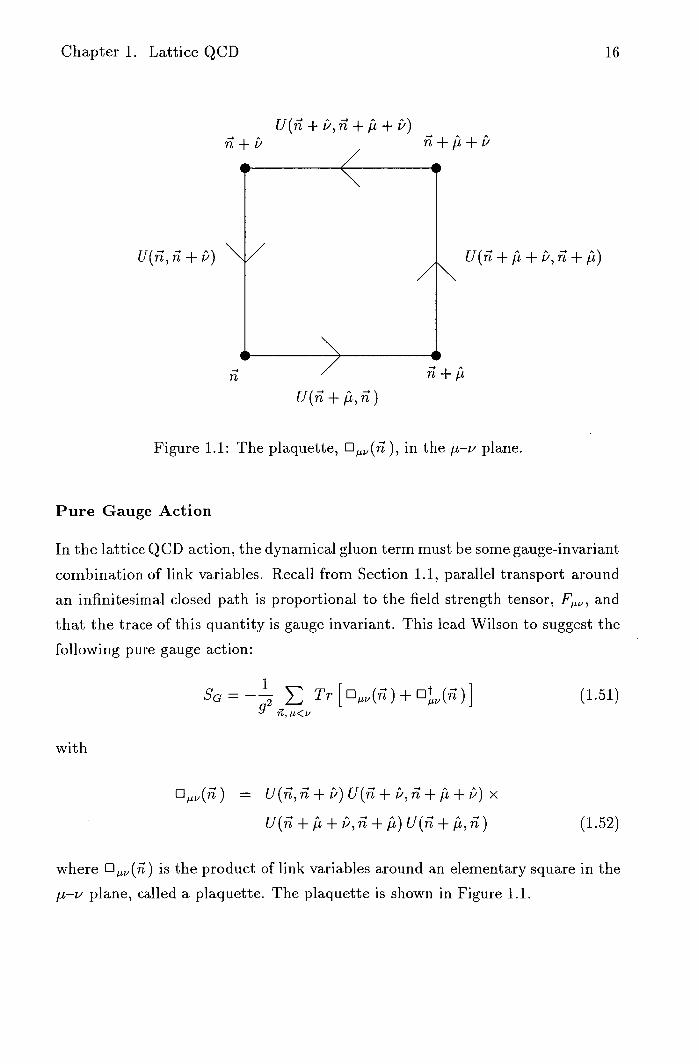
Pseudoscalar Two-Point Functions
Taking F = 'y 5 in Eqn. (1.83) gives the following pseudoscalar operators:
P(x) = it(x)'y 5 1(x) (1.87)
pt(x ) — T(x)'y 5 h(x) (1.88)
where the flavour notation h and I is used to denote a 'heavy' and 'light' quark
respectively. Substituting these operators into Eqn. (1.85) one obtains the heavy-
light pseudoscalar two-point function
G 2 (t, 0; ) = - e t (0 { jx)_ Y 5 ,6 1(x) T(0) h(0)} o). (1.89)
The time-ordered product of field operators in Eqn. (1.89) is related by Wick's
theorem [43] to the following product of quark propagators
(0(x)M(0)l0)(0l((0)0)&+ (1.90)16
where terms with zero vacuum-expectation-value simply vanish. Using Eqn. (1.70)
and the following hermiticity property of the lattice quark propagator
Qt(x,0;U) = QS (0,x;U)y so (1.91)
one obtains the heavy-light pseudoscalar correlator in terms of quark propagators
G 2 (t, 0;) = ( Tr[ Ht(x,0;U) L(x, 0;U)] ) (1.92)
where the trace is over both spin and colour, and ( ... ) denotes an average over
gauge configurations, U. The 'H'-eavy and 'L'-ight propagators in Eqn. (1.92)
are both computed for a fixed origin.

Chapter 1. Lattice QCD
25
- rrff i-.\ -
V
r F
_\, I
Figure 1.3: The heavy-light meson correlator.
Vector Two-Point Functions
Taking F = in Eqn. (1.83) gives the following vector operators:
VI x) = ii(x)-yl(x) (1.93)
Tt(x) = — 1(x)yh(x). (1.94)
Substituting these operators into Eqn. (1.85) one obtains the following heavy-light
vector correlator in terms of quark propagators
(i, 0; ) = K Tr{ 5 H(x, 0;U) L(x, 0; U) )
(1.95)
where the trace is over both spin and colour, and ( ... ) denotes an average over
gauge configurations, U. The 'H'-eavy and 'L'-ight propagators in Eqn. (1.95) are
both computed for a fixed origin. Figure 1.3 shows a heavy-light meson correlator
constructed from quark propagators.
1.6 Meson Masses
At large Euclidean times, meson correlation functions have a simple analytic form
which can be parameterised by an overall normalisation factor and the mass of
the corresponding particle. This section describes the time-dependence of both
pseudoscalar and vector meson correlators, given in Section 1.5.

Chapter 1. Lattice QCD 26
Meson Correlators
Inserting a complete set of states in Eqn. (1.85) gives
G(t,0;) = ,s,2cEs()
(0 M(, ,10)o) (1.96)4.
with the lattice completeness relation defined as follows:
1
L 2s(P) S,p)(S,p + (1.97)
S,
where the sum S is over all single-particle states; the omitted terms correspond
to multi-particle states.
Under the following symmetry transformation
QM(x) -~ 1(x) = eM(0)e" (1.98)
with
X=aHt+i-L-73.x (1.99)
where H and P are the lattice Hamiltonian and the three-momentum operator
respectively. These operators act on adjacent states in Eqn. (1.96) to give
Gk(t, 0; j) = (1.100) 2aEs(7)
X q JQI
Finally, using the definition of the lattice delta function
•) it(_cfl. (1.101)
one obtains the following expression for the meson correlator
2
cM(t;P)=2E() X(0M(0)S,P) (1.102)

Chapter 1. Lattice QCD
27
where there is now an explicit time-dependence. The only non-zero contribution
to this sum are the ground state meson and its excitations. These higher-energy
excitations fall off exponentially compared to the ground state which gives the
dominant contribution as t -+ oo.
Pseudoscalar Correlator
At large Euclidean times, the pseudoscalar meson correlator is given by
e_Ep()t 2 Cp(t;p)
2aEp() x (1.103)
t — oo
with
Zp(p) (0P(0)P, g ) (1.104)
where Ep is the energy of the pseudoscalar meson with lattice three-momentum
A and Zp is the corresponding two-point amplitude. This amplitude measures
the overlap of the interpolating operator P with the pseudoscalar meson state, P.
Vector Correlator
At large Euclidean times, the vector meson correlator is given by
CJLV (1.105)
r=1 2aEv() t—+00
X
where Ev is the energy of the vector meson with lattice three-momentum j5. The
vector correlator is slightly more complicated than the pseudoscalar case because
Eqn (1.105) contains an additional sum over polarisation states, r.
Writing the vector amplitude with an explicit polarisation vector as follows:
(0(0)) )Zv ()
(1.106)
where Zv is the vector meson two-point amplitude; and using the following

Chapter 1. Lattice QCD 28
polarisation sum identity for a massive vector particle
3 p/pL' _glLU
+ rn2 (1.107)
r1
one obtains the following form for the vector meson correlator
pLpV )
C(t;)= (—g + 2aEv()
Zv( 2 . ( 1.108)
Contracting Eqn. (1.108) with the Euclidean metric, and using the on-shell con-
dition PPji, m 2 , one obtains the polarisation-averaged vector meson correlator
e_aEu1 ()t 2
Cv(t;j) ) —3 x x Zv( (1.109) 2a Ev()
t — oo
which differs in form from the pseudoscalar correlator, given by Eqn. (1.103), by
a simple factor of (minus) 3. This factor corresponds to the three polarisation
states of the vector particle.
1.7 Three-Point Functions
On the lattice, matrix elements are extracted by studying the time-dependence of
correlation functions. This section describes how to construct three-point func-
tions corresponding to the semi-leptonic decay of both pseudoscalar and vector
heavy-light mesons into pseudoscalar mesons.
Three-Point Functions
The three-point function describing the semi-leptonic decay of meson A into meson
B is defined as follows:
G2B(t Y ,tX, 0;, ) = 0 1 11 {B(y) J(x) At(0)} 1 0) (1.110)
where At and B are the meson creation and annihilation operators respectively,
and J is the weak current operator. In Eqn. (1.110) the outgoing meson, B, has
lattice three-momentum j, and is the momentum-recoil from the weak decay.
The incoming meson, A, has lattice three-momentum (j+ fl.

Chapter 1. Lattice QCD 29
The semi-leptonic decay of a heavy-light meson proceeds as follows: the heavy
quark decays into a 'lighter' quark via the weak interaction; and independently of
the light quark, 1. This suggests the following weak current operator
J(x) = h'(x)A"h(x) (1.111)
with
AO = 'y' (1 -,y 5) (1.112)
where h' and h denote two distinct 'heavy' quark flavours. Following Section 1.5,
the meson operators are given by
A(x) = —1(x) F'h'(x) (1.113)
B(x) h(x)y 5 1(x) (1.114)
where B is the interpolating operator to annihilate a heavy-light pseudoscalar
meson. At is the interpolating operator to create a pseudoscalar or vector heavy-
light meson with F = or = ny" respectively.
Pseudoscalar-to-Pseudoscalar Decay
For the pseudoscalar decay, taking F = y5 in Eqn. (1.110) gives
G(t,t,0;,fl = (1.115) , .
X (üj { (y) 5 1(y) '(x)Ah(x) T(0)5h'(0) } 0).
Applying Wick's theorem, and using Eqns. (1.71) and (1.91), one obtains the
pseudoscalar-to-pseudoscalar three-point correlator in terms of quark propagators
't t,0;j7,) = (1.116)
x (Tr,,, [Hlt(x, 0;U) 5 A H(x, y;U)L(y, 0;U)] )
where the trace is over both spin and colour, and (.. •) denotes an average over
gauge configurations, U.

L(y,0)
rAL 5ffFt(x 0')-y5
F 11
H(xj)
-y 5
Chapter 1. Lattice QCD
30
Figure 1.4: The three-point correlator.
Vector-to-Pseudoscalar Decay
Similarly, taking F11 = y 11 in Eqn. (1.110) one obtains the vector-to-pseudoscalar
three-point correlator in terms of quark propagators
2ir f_(3)ivft t,0;i57) = (1.117) LTv_+p v'
X K Tr s , c [ 5 H't (x ) 0;U) 5 A H(x, y; U) 5 L(y, 0;U)] )
where the trace is over both spin and colour, and denotes an average over
gauge configurations, U. Figure 1.4 shows the three-point correlator constructed
from quark propagators.
The heavy quark propagator H(x,y;U), in Eqns. (1.116) and (1.117), requires
the inversion of the entire fermion matrix which is computationally prohibitive.
Fortunately, three-point correlators can be constructed using an extended quark
propagator computed for a fixed origin. In practice, the three-point correlator is
computed as a function of t x with t a constant. This corresponds to varying the
position of the weak current operator between two fixed mesons.

Chapter 1. Lattice QCD 31
Extended Quark Propagator
The extended quark propagator is defined as follows:
qf (x, 0; t;U) > effH(x, y;U) y 5 L(y, 0;U) (1.118)
where the sum is over the spatial dimension, W. Eqn. (1.118) can be rewritten in
the following matrix notation
(x ) 0; t; U) = 8(t, t) et7 H(x, Z; U) 75 L(z, 0;U) (1.119)
where there is now an implied sum over (, ti).
Multiplying both sides of Eqn (1.119) by the heavy fermion matrix one obtains
H 1 (z, x;U) çf(x, 0; t;U) = 7]SEQ(z) 0) (1.120)
with
1sEQ(z) 0) = 8(t, t,) e L L(z, 0; U) (1.121)
which is in the standard form for fermion matrix inversion, given by Eqn. (1.75).
71SEQ(x1 0) is called the 'sequential' source [44] and is essentially just the t-th
time-slice of the light propagator, L(x, 0; U). Thus, three-point correlators can be
constructed from quark propagators computed for a fixed origin, and there is no
need to invert the entire fermion matrix. The extended propagator is denoted in
Figure 1.4 by the bold 'propagator' line.
1.8 Weak Matrix Elements
At large Euclidean times, three-point correlation functions have a simple analytic
form which can be parameterised by various two-point quantities (the masses
and amplitudes from Section 1.6) and the corresponding matrix element. This
section describes the time-dependence of both the pseudoscalar-to-pseudoscalar
and vector-to-pseudoscalar three-point correlators, given in Section 1.7.

Chapter 1. Lattice QCD
32
Three-Point Correlators
Inserting two complete sets of states in Eqn. (1.110) gives
1 eT' 1 eT
g, S 1 ,
CB(t,tX,0;) x- = L3 2a ES, ( k i ) L 3 k;2aEs2 ()
(0jB(y)S i ,k)( S i , J(x)S2,)
>< (S2 ,k 2 iAt(0)o). (1.122)
Using translation symmetry, to shift the operators B(y) and J(x) to the origin,
one obtains the following three-point correlator
aE51 () (t—t)
G B (t Y 1 tX,0;) = Si 2a Es, x
2a Es, (+)
• (oB(o)S 1 , )( s1 , J(0)S2,+)
• (S2 ,+At(0)0) (1.123)
where there is now an explicit time-dependence. The only non-zero contribution
to this sum are the ground states of the incoming and outgoing mesons, and their
excitations. These higher-energy excitations fall off exponentially compared to
the ground states which give the dominant contributions as (t — t) —+ cio and
Pseudoscalar-to-Pseudoscalar Time-Dependence
At large Euclidean times, with t = T fixed, the pseudoscalar-to-pseudoscalar
three-point correlator is given by
(T—t) e aE(flt Z)
2aEQ) x Z+
2aE(j+ )
x (Bp, J(0)Ap,1+) (1.124)

Chapter 1. Lattice QCD 33
where (Be , J(0) A, 3+ ) is the weak matrix element describing the semi-
leptonic decay of pseudoscalar meson A into pseudoscalar meson B. Ep and Zp
are the corresponding energies and two-point amplitudes respectively.
Vector to Pseudoscalar Time-Dependence
At large Euclidean times, with t,, = T fixed, the vector-to-pseudoscalar three-point
correlator is given by
eaE() (T—t) cpL(t;p,q;T) ,'
2aEpB(1i) (1.125)
( )t e_a X ZQ5-i-) x 7iW
2a E+ )
with 3
+) (1.126) r1
where JIW is the polarisation-averaged weak matrix element describing the semi-
leptonic decay of vector meson A into pseudoscalar meson B. E and Z are the
corresponding energies and two-point amplitudes of the pseudoscalar and vector
mesons.
Chapter 2
Meson Spectrum
This chapter describes a lattice calculation of the meson spectrum. Lattice results
are presented for both the light-light and heavy-light mesons. These results are
extrapolated to the physical masses and compared with experiment.
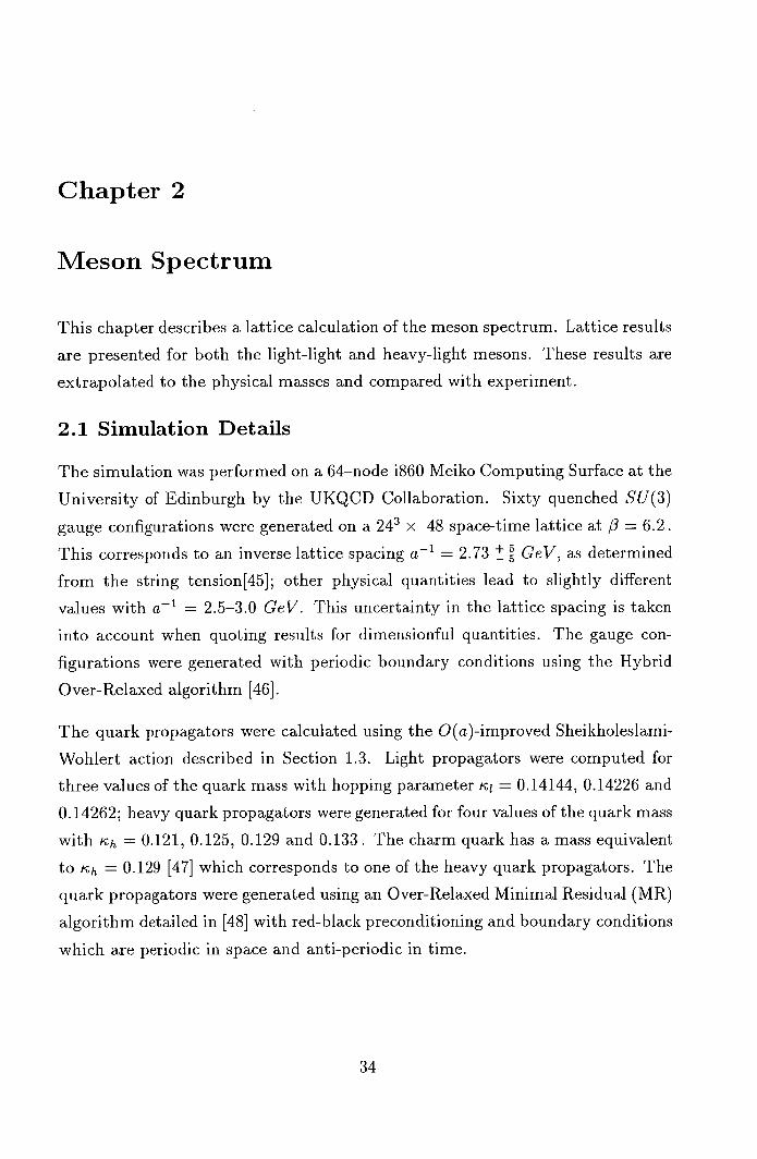
2.1 Simulation Details
The simulation was performed on a 64—node 1860 Meiko Computing Surface at the
University of Edinburgh by the UKQCD Collaboration. Sixty quenched SU(3)
gauge configurations were generated on a 24 x 48 space-time lattice at 0 = 6.2.
This corresponds to an inverse lattice spacing a 1 = 2.73 +' GeV, as determined
from the string tension[45]; other physical quantities lead to slightly different
values with a 1 = 2.5-3.0 GeV. This uncertainty in the lattice spacing is taken
into account when quoting results for dimensionful quantities. The gauge con-
figurations were generated with periodic boundary conditions using the Hybrid
Over-Relaxed algorithm [46].
The quark propagators were calculated using the 0(a)-improved Sheikholeslami-
Wohlert action described in Section 1.3. Light propagators were computed for
three values of the quark mass with hopping parameter 'i = 0.14144, 0.14226 and
0.14262; heavy quark propagators were generated for four values of the quark mass
with kh = 0.121, 0.125, 0.129 and 0.133. The charm quark has a mass equivalent
to Kh = 0.129 [47] which corresponds to one of the heavy quark propagators. The
quark propagators were generated using an Over-Relaxed Minimal Residual (MR)
algorithm detailed in [48] with red-black preconditioning and boundary conditions
which are periodic in space and anti-periodic in time.
34

Chapter 2. Meson Spectrum
35
2.2 Statistical Analysis
Recall from Sections 1.6 and 1.8, at large Euclidean times two-point and three-
point correlators are described by analytic functions of the meson masses and
matrix elements. These parameters can be extracted by fitting correlators to
appropriate model functions. Recall from Sections 1.5 and 1.7, correlators are
constructed from quark propagators computed for a finite number of gauge con-
figurations. To estimate the error on a fit parameter, the simulation should ideally
be repeated (many times) for different gauge configuration samples. In practise,
this is prohibitive since both gauge configurations and quark propagators are com-
putationally expensive. The error on a fit parameter can instead be estimated
using the Jackknife and Bootstrap methods [49].
Jackknife Error
The jackknife error, cr, on a quantity P computed from a data set Y with n data
elements, Y1, Y2) . . . , y,, is defined as follows:
n
(2.1) i= 1
with
(pi)= 1 p
(2.2)
where pi is the quantity P computed from the i—th jackknife sample (Y - y) with
(n — i) data elements, Y1,Y2,. . . , Yi-1,Y+1,... ,y.
The quantity P and its jackknife error are quoted as follows:
P+ UP
(2.3)
The normalisation factor in Eqn. (2.1) is included to make the jackknife give
the 'right' answer for the standard deviation, o; in which case the quantity P is
simply the average of the data set. The standard deviation formula of elementary
statistical analysis [50] assumes the data is normally distributed. The jackknife
method makes no such assumption and is therefore suited to situations in which
the distribution of the data is unknown.

Chapter 2. Meson Spectrum co
Bootstrap Error
The bootstrap error, o, on a quantity P computed from a data set Y with n
data elements, Yi, Y2.... , y, is defined as follows:
B
= ____ 2
(2.4) O'P
with a* and b*, the lower and upper bounds respectively, chosen such that
1—C {pj<b*} 1+C and = (2.5)
N 2 N 2
where pi is the quantity P computed from the i—th bootstrap sample, N is the
number of bootstrap samples, C is the confidence level in the range [0, 1], and
of ...} denotes the number of p i satisfying the enclosed relation. Each bootstrap
sample consists of n data elements selected at random from Y with replacement.
The quantity P and its bootstrap error are quoted as follows:
D+ B I - O p . (2.6)
Typically, a* and b* are computed with a 68% confidence level (C = 0.68). For a
normal distribution, this is the percentage of measurements which lie within one
standard deviation of the mean. The accuracy in the bootstrap estimate of the
error increases with the number of bootstrap samples.
Correlator Data
Recall from Section 1.4, quark propagators are computed on a space-time lattice
for a fixed number of gauge configurations. And recall from Sections 1.5 and 1.7,
correlators are constructed, timeslice by timeslice, by combining quark propaga-
tors and averaging (with an appropriate phase factor) over the spatial dimensions
of the lattice. Correlator data is stored in an array with the following dimensions:
data[c][n][t] (2.7)
where c is the number of correlators, n is the number of gauge configurations and
t is the number of timeslice components.
Chapter 2. Meson Spectrum
37
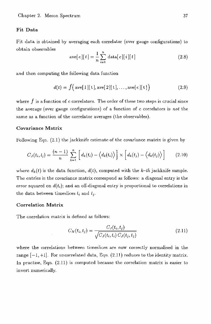
Fit Data
Fit data is obtained by averaging each correlator (over gauge configurations) to
obtain observables
ave[c][t]=data[c][i][t] (2.8)
and then computing the following data function
d(t) = f(ave[1][t],ave[21[t],. . .,ave[c][t]) (2.9)
where f is a function of c correlators. The order of these two steps is crucial since
the average (over gauge configurations) of a function of c correlators is not the
same as a function of the correlator averages (the observables).
Covariance Matrix
Following Eqn. (2.1) the jackknife estimate of the covariance matrix is given by
(n 1) C(t,t) = - (dk(t))] - (d(t))] (2.10)
k=1
where dk(t) is the data function, d(t), computed with the k—th jackknife sample.
The entries in the covariance matrix correspond as follows: a diagonal entry is the
error squared on d(t); and an off-diagonal entry is proportional to correlations in
the data between timeslices t i and t.
Correlation Matrix
The correlation matrix is defined as follows:
CN(t,t) C(t,t)
(2.11) =
where the correlations between timeslices are now correctly normalised in the
range [-1, +1]. For uncorrelated data, Eqn. (2.11) reduces to the identity matrix.
In practise, Eqn. (2.11) is computed because the correlation matrix is easier to
invert numerically.

Chapter 2. Meson Spectrum
Fit Procedure
Consider the most general case: fitting an analytic model function, f(t; ),
parameterised by m parameters, a 2 = a 1 , a 2 ,.. . , a, to a data function, d(t). The
fit is performed by minimising the following chi-squared function with respect to
the model parameters, Z:
= [f(tj; ) - d(t)] x CJ1 (t i , t) x [f(tj; ) - d(t)] (2.12) ti, t,
where CJ1 (t, t) is the inverse of the jackknifed covariance matrix. The min-
imisation of Eqn. (2.12) is performed numerically using a Marquardt- Levenberg
algorithm [51].
Fit Parameter Errors
To estimate the errors on the model parameters, a, the entire fit procedure is
repeated with N bootstrap data sets. For each bootstrap sample, both the
data function afid the covariance matrix are re-computed using Eqns. (2.8-2.9)
and (2.10) respectively. In practice, both the best-fit parameters, a, and the N
bootstrap values are stored. The error on a particular parameter, a, is computed
(when required) using Eqn. (2.4).
All correlators are computed from the same sixty SU(3) gauge configurations.
This data is likely to be highly correlated. Hence, all fit parameters are determined
from correlated chi-squared fits. The error quoted on all quantities corresponds to
a 68% confidence level, on a distribution obtained from 1000 bootstrap samples.
The x 2 /dof is quoted as an indicator of the goodness-of-fit. The number of degrees
of freedom (dof) is given by
dof = (t - m)
(2.13)
where m is the number of model parameters and t is the number of timeslices
included in the fit. As a rule of thumb a x 2/dof 1 indicates a good fit to the
data.

Chapter 2. Meson Spectrum
39
2.3 Two-Point Correlator Fits
Recall from Section 1.5, the pseudoscalar and the vector meson correlator are
constructed from quark propagators using Eqns. (1.92) and (1.95) respectively.
And recall from Section 1.6, at large Euclidean times these correlators are given
by Eqns. (1.103) and (1.109).
Meson Fit Function
The ground-state energy, E, and the corresponding two-point amplitude, Z, are
extracted by fitting the meson correlator to the following fit-function:
C(t) = A {e_Bt + 6—B (T - t)} (2.14)
where the terms e_Bt and e_B(T_t) represent the 'forward' and 'backward' propa-
gating particles respectively', and T is the temporal extent of the lattice. The fit
parameters A and B are related to the ground state energy and the corresponding
two-point amplitude by
A = z2 and B = E. (2.15)
For an infinite number of gauge configurations, the meson correlator is exactly
mirrored about the mid-point of the lattice. This is a consequence of the boundary
conditions and time reversal symmetry. Prior to fitting, the configuration data
is 'folded' by averaging the corresponding timeslices from the two halves of the
lattice. In this study, T = 48 and the data is folded about t = 24. This procedure
improves statistics by effectively doubling the number of gauge configurations.
The vector data is averaged over polarisation states and divided by a factor of 3.
The values of momenta on a lattice of spatial volume L 3 , with periodic boundary
conditions, are quantised and given by Eqn. (1.26). For L = 24, the allowed values
of momenta are given by -. P = --- (nm, n,,, n) (2.16)
12 a
where m, n and r are integers.
'For meson correlators these particles are identical.

Chapter 2. Meson Spectrum 40
To increase statistics, the correlator data is averaged over all equivalent
momentum channels before fitting. For example, the channels (1,0,0), (0,1,0)
and (0,0,1) are equivalent and their average corresponds to a particle with
momentum j = ir/12a. The UKQCD data set corresponds to particles with
the following momenta: jI = 0, 1, \/a and 2, in units of 7r/12 a.
Light-Light Masses
The UKQCD propagator set contains three light quark masses with hopping
parameter 'i = 0.14144, 0.14226 and 0.14262. These kappa values allow the con-
struction of six independent light-light correlators for both the pseudoscalar and
vector mesons. The masses and two-point amplitudes, obtained from fits to zero
momentum correlators, are given in Tables 2.1 and 2.2 respectively. For the pseu-
doscalar channel the fit interval is t = 14-22; and for the vector channel t = 13-23.
These fit ranges were determined in an earlier UKQCD study [45]. The chi-squared
values in Table 2.1 indicate a good fit (x2/dof 1) for all kappa combinations.
Fits to meson correlators with non-zero momentum were also performed; the
corresponding energies and two-point amplitudes are required to extract three-
point matrix elements over a range of momentum transfer. The noise in the
two-point correlator signal increases rapidly with momentum because the number
of gauge configurations is finite. In the pseudoscalar case, a fit to any correlator
with lattice momenta greater than units of 7r/12 a either fails or gives an
unacceptable chi-squared (x 2 /dof >> 1).
In Figure 2.1 the pseudoscalar energy is plotted as a function of the momentum
squared. This data is fitted to the continuum dispersion relation given by
E=m2 +I 2 (2.17)
where only the first three data points are included in each fit. Figure 2.1 shows
the dispersion relation is well-satisfied for pseudoscalar meson correlators with
momentum < 702 a. The fitted masses are also in excellent agreement with the
values obtained from the zero-momentum correlators, given in Table 2.1.

Chapter 2. Meson Spectrum
41
'12 Pseudo x 2 /dof Vector x 2 /dof
0.14144 0.14144 0.298 ii 1.24 0.395 ii 1.82
0.14144 0.14226 0.259 j 0.90 0.370 t 1.35
0.14144 0.14262 0.241 t 0.76 0.360 ji 1.01
0.14226 0.14226 0.214 jj 0.99 0.343 0.86
0.14226 0.14262 0.192 ii 0.99 0.331 ji 0.60
0.14262 0.14262 0.167 + 3 1.04 0.319 j 0.44
0.1418 j 0.14315 + 2 0.186 it 1.37 0.331 ji 13
0.42 0.14315 j 0.14315 0 2.30 0.290 ii
13
Table 2.1: Light-light meson masses in lattice units; for the pseudoscalar channel the fit is over the time interval t = 14-22; and for the vector channel the fit is over the time interval t = 13-23. The values quoted in the lower half of the table correspond to the pseudoscalar and vector masses extrapolated to K,, = 0.14315 ji and ,i = 0.1418ji 1
1
KI, K12 11 Z(Ipl = 0) Z(p 0)
0.14144 0.14144 0.0081 it 0.0025 it
0.14144 0.14226 0.0067 ji 0.0021 i
0.14144 0.14262 0.0062 i 0.0019 it
0.14226 0.14226 0.0056 0.0017 it
0.14226 0.14262 0.0052 ii 0.0015
Table 2.2: Light-light meson two-point amplitudes. The fit ranges and x 2 /dof are the same as those in Table 2.1.

Chapter 2. Meson Spectrum
1.0
L—L Pseudo Dispersion Eel.
reI;I O Mfit = 0.297 +
1'
El Mfit = 0.19
T0.6 02
> 0.4
Ic 1 = 0.14144 0
Ic 1 = 0.14144 2
ic1 = 0.14226 El '
ic j2 = 0.14262
0 1 2 3 4
p1 2 / ( rr/12a)2
Figure 2.1: Light-light pseudoscalar dispersion relation.
1.5
c1.0
N 0.5
SIM
L—L Pseudo 2pt Amp
= 0.14144 Ic
12 = 0.14144
ICII = 0.14226 IG
12 = 0.14262
0 Zfit = 0.00131 +3
- +2 0 Z = 0.0050 -
0 1 2 3 4
1p1 2 / (7T/12a)2
0.2
ME
42
Figure 2.2: Light-light pseudoscalar two-point amplitudes.

Chapter 2. Meson Spectrum 43
In Figure 2.2 the pseudoscalar two-point amplitude is plotted as a function of the
momentum squared. This data is fitted to a constant: the two-point amplitude
should be independent of momentum for meson correlators constructed from local
interpolating operators. The fitted Z 2 are in excellent agreement with the values
obtained from the zero-momentum correlators given in Table 2.2.
Heavy-Light Masses
The UKQCD propagator set contains a heavy quark mass with hopping parameter
= 0.129 corresponding to the mass of the charm quark, and light quark masses
with hopping parameter ic 1 =0.14144, 0.14226 and 0.14262. These kappa values
allow the construction of three independent heavy-light correlators for both the
pseudoscalar and vector mesons.
The heavy quark propagator is smeared at both the source and sink using gauge
invariant Jacobi smearing described in Section 1.4. Correlators constructed from
smeared quark propagators correspond to spatially-extended interpolating oper-
ators which help isolate the ground state mass. In the 'static' limit (infinite
heavy-quark mass), the use of such operators is essential to obtain any signal.
The masses and two-point amplitudes, obtained from fits to zero-momentum
correlators, are given in Tables 2.3 and 2.4 respectively. For both the pseudoscalar
and vector channel, the fit interval is t = 11-22. This fit range was determined
in an earlier UKQCD study [47]. The chi-squared values in Table 2.3 indicate a
good fit (x 2 /dof 1) for all kappa combinations.
In Figure 2.3 the pseudoscalar energy is plotted as a function of the momen-
tum squared. This data is fitted to the continuum dispersion relation given by
Eqn. (2.17) where the fit includes all data points. The dispersion relation is well-
satisfied for all heavy-light correlators; all data points are within two sigma. The
fitted masses are also in excellent agreement with the values obtained from the
zero-momentum correlators, given in Table 2.3.
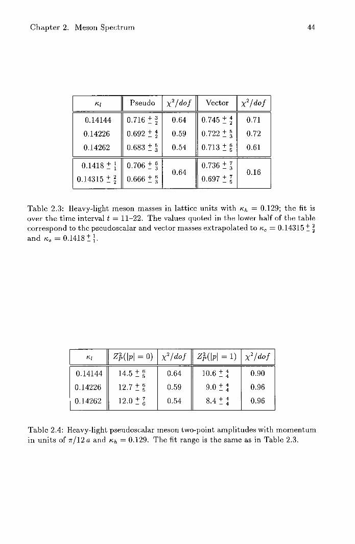
Chapter 2. Meson Spectrum 44
KI Pseudo x 2 /dof Vector _ [Tdof]
0.14144 0.716 0.64 0.745 0.71
0.14226 0.692 i 0.59 0.722 0.72
0.14262 0.683 + 5 0.54 0.713 ii 0.61
0.1418 0.706 0.736 II 0.64 0.16
0.14315 0.666 0.697
Table 2.3: Heavy-light meson masses in lattice units with ich = 0.129; the fit is over the time interval t = 11-22. The values quoted in the lower half of the table correspond to the pseudoscalar and vector masses extrapolated to K, = 0.14315 and ,i = 0.1418i .
KI ~ j Z,2 (Ip = 0) x 2 /dof Zp = 1) x 2 /dof
0.14144 14.5 i 0.64 10.6 0.90
0.14226 12.7 t 0.59 9.0 t 0.96
0.14262 12.0 ii 0.54 8.4 i!i 0.96
Table 2.4: Heavy-light pseudoscalar meson two-point amplitudes with momentum in units of 7r/12a and Kh = 0.129. The fit range is the same as in Table 2.3.

Chapter 2. Meson Spectrum
45
111 1 11! - H—L Pseudo Dispersion Rel.
- 0.717
11 rn f1 =0.681t
ICh = 0.12900 -
0 Ic1 = 0.14144
D /c1 = 0.14262
1.0
0.9
CQ + E0.8
0.7
SL1 0 1 2 3 4
p1 2 / (7T/12a)2
Figure 2.3: Heavy-light pseudoscalar dispersion relation.
20 I I I I I I I I II 11 1 111 H—L Pseudo 2pt Amp
15 0 IC1 = 0.14144
( IC1 = 0.14262
'- 10 +
Eu
5 w /C h = 0.12900 W
0 0 1 2 3 4
1p1 2 / (7r/12a)2
Figure 2.4: Heavy-light pseudoscalar two-point amplitudes.

Chapter 2. Meson Spectrum 46
In Figure 2.4 the pseudoscalar two-point amplitude is plotted as a function of the
momentum squared. The momentum dependence of the heavy-light two-point
amplitude is a feature of using spatially-extended interpolating operators. The
overlap with the ground state decreases with increasing momentum because the
volume of the smeared 'wave-function' is Lorentz contracted along the direction
of motion.
For non-zero momentum, heavy-light meson correlators are fitted by constraining
the two-point energy to values computed from the continuum dispersion relation
using the masses in Table 2.3. Thus, a single parameter fit is used to determine
the two-point amplitudes for correlators with non-zero momentum. The data in
Figure 2.4 is obtained by this method. The two-point amplitudes, obtained from
one parameter fits to heavy-light meson correlators with= 7r/12 a, are given
in Table 2.4.
Three-point correlator fits (discussed in the following chapters) are particularly
sensitive to two-point quantities. Thus, two-point energies are computed from
the masses quoted in Tables 2.1 and 2.3 using the continuum dispersion relation;
light-light two-point amplitudes are constrained to their zero-momentum values,
quoted in Table 2.2; and heavy-light two-point amplitudes are obtained from one-
parameter fits (described above), quoted in Table 2.4.
2.4 Chiral Extrapolation
This section describes how the physical meson masses are obtained from the lattice
light-light and heavy-light data. Recall from Section 1.2, in the Wilson formulation
the bare quark mass is given by
i/i
2k m= — I ---
I ) (2.18)
where n, is the hopping parameter corresponding to zero quark mass. For each
quark flavour, a hopping parameter must be found which corresponds to the
physical value. The light quarks u and d are assumed to be degenerate in mass
(corresponding to an exact isospin symmetry) with Ic1, = r1d =

Chapter 2. Meson Spectrum 47
Light-Light Pseudoscalar Extrapolation
The light-light pseudoscalar meson obeys the following PCAC [2] relation:
Mp DC Mq (2.19)
where m q is the mass of the constituent light quarks. Using Eqn. (2.18), the
mass-dependence of the light-light pseudoscalar data is given by
MP (id1) 1d12 ) = b (-±_ -
( 2.20) 1d eff 'cc )
with
- 1 1 ( 1 -+ 1 "
- 1 - ( 2.21) -
Id eff 2 '12) 2 ice, '12
where bp and n, are free parameters, and Ideff is an effective kappa corresponding
to an average of the constituent quark masses. In this model, ic e, is the hopping
parameter for which the pion mass vanishes.
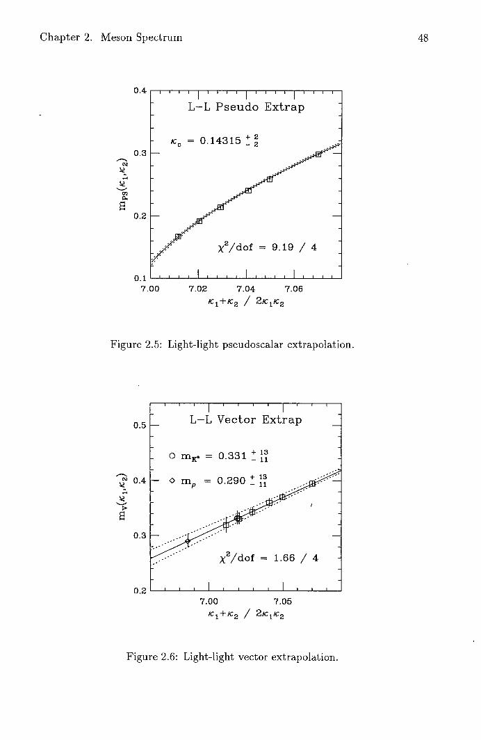
Figure 2.5 shows the light-light pseudoscalar data, quoted in the upper-half of
Table 2.1, plotted as a function of the inverse effective-kappa. This data is fitted
to Eqn. (2.20) to obtain
= 0.14315 t (2.22)
where the fit chi-squared (x2/dof 2), although a little high, is still acceptable.
The pion mass, given by Eqn. (2.20) with ic = ' i2 = ic e , is zero by definition.
This value and the fit chi-squared are quoted in the lower-half of Table 2.1.
Light-Light Vector Extrapolation
The light-light vector meson is assumed to be linear in the light quark masses
mv(1d11, K12)= av + b - ( 2.23) k'dej Idc)
where av and bV are free parameters.
Chapter 2. Meson Spectrum
0.4
L—L Pseudo Extrap
IC 0 = 0.14315 +2-2
0.3 CQ
Ca
-I
0.2
X 2/dof = 9.19 / 4
0.1 7.00
7.02 7.04 7.06 #c 1 +/c2 / 2,c/c 2
Figure 2.5: Light-light pseudoscalar extrapolation.
0.5 L—L Vector Extrap
- o MK' =O.33111
0.4 - Om =0.290i
0.3
X2/dof = 1.66 / 4
0.2 7.00 7.05
Icl+1c2 / 2,c1/c2
Figure 2.6: Light-light vector extrapolation.

Chapter 2. Meson Spectrum 49
Figure 2.6 shows the light-light vector data, quoted in the upper-half of
Table 2.1, plotted as a function of the inverse effective-kappa. This data is fitted
to Eqn. (2.23) to obtain
MP = 0.290 (2.24)
where av and bV are determined by the fit. The chi-squared (x2/dof 0.4)
indicates a good fit to the data. The rho mass, m p , is computed from Eqn. (2.23)
with i = K12 = This mass and the fit chi-squared are quoted in the lower-half
of Table 2.1. Figure 2.6 includes two extra data points corresponding to the mass
of the p and K* mesons.
Light-Light Ratio Extrapolation
The hopping parameter i, corresponding to the mass of the strange quark, is
required to study the effects of SU(3) symmetry breaking on the meson spectrum.
A value for t is determined by fitting the ratio m2p(/c11, r,12) / m to some function
of the light quark masses; extrapolating 'i1 to ii; and using k1 2 to fix the ratio to
the experimental value m'/m. The light-quark dependence of m(icl 1 , 'l2) / m
is given by Eqn. (2.20) since m is just a constant.
The ratio data is computed from the light-light pseudoscalar masses and the
light-light vector extrapolated rho mass, quoted in the upper and lower halves
of Table 2.1 respectively. Figure 2.7 shows the ratio data plotted as a function of
the inverse effective-kappa, and fitted to Eqn. (2.20) to obtain
K S = 0.1418k with = 0.413 (2.25) m
where the fit chi-squared (x2/dof = 1.4) indicates a fairly good fit to the data.
Using Eqns (2.20) and (2.23), to compute the K and K* meson masses
respectively, gives
MK = 0.186 iand MK- = 0.331 t (2.26 )
with 'i1 = and Ici2 = r,,. These masses and the corresponding fit chi-squared
are quoted in the lower-half of Table 2.1.

Chapter 2. Meson Spectrum 50
I I I I I I I I I I I I I I
L—L Pseudo Extrap
!c=0.1418
Y2 /Zdof 6.86 5
I I I I I I
1.5
Q.
1.0
N
Q..
0.5
7.00 7.02 7.04 7.06
ic 1 -I-#c 2 / 2/c 1 /c 2
Figure 2.7: Light-light ratio extrapolation.
NM I I I I I I I I I I
H—L Pseudo Extrap
0.75 - 'mD =0.666ii -
N
0 M = 0.706t ...<
0.70
0.65
X 2/dof = 0.64 1 -
I I I I I I
6.95 7.00 7.05 7.10
1 / ,c 1
Figure 2.8: Heavy-light pseudoscalar extrapolation.

Chapter 2. Meson Spectrum
51
Heavy-Light Pseudoscalar Extrapolation
Both the pseudoscalar and vector heavy-light mesons are assumed to be linear in
the light quark mass
mp(kl) mv() = a'+ b' - ( 2.27) 'i ,c)
where a' and b' are free parameters.
Figure 2.8 shows the heavy-light pseudoscalar data, quoted in the upper-half of
Table 2.3, plotted as a function of the inverse light-kappa. This data is fitted to
Eqn. (2.27) to obtain
MD = 0.666 iand MD = 0.706 ii (2.28)
where the fit chi-squared (x 2 /dof = 0.6) indicates a good fit to the data.
The D and D3 meson masses are computed from Eqn. (2.27) with 'i =
and 'i = r., respectively. These masses and the fit chi-squared are quoted in
the lower-half of Table 2.3.
Heavy-Light Vector Extrapolation
The vector heavy-light data, quoted in the upper-half of Table 2.3, is fitted to
Eqn. (2.27) to obtain
rnD* = 0.697 iand mD* = 0.736 (2.29)
where the fit chi-squared (x2/dof = 0.2) indicates a good fit to the data.
The D* and D meson masses are computed from Eqn. (2.27) with 'i =
and 'i = ic 9 respectively. These masses and the fit chi-squared are quoted in the
lower-half of Table 2.3. From Eqns. (2.28) and (2.29), it is clear that this lattice
calculation is sensitive to SU(3) symmetry breaking effects in the heavy-light
meson spectrum.

Chapter 2. Meson Spectrum
52
2.5 Physical Meson Spectrum
The meson masses, up till now, have been quoted in lattice units (a = 1). The
masses quoted in Table 2.5 are in physical units with a 1 = 2.85 ii 0.15 GeV. This
value includes an estimate of the error in the determination of the inverse lattice
spacing from different quantities. This uncertainty is the largest source of error
in the lattice calculation. The experimentally measured masses [52] are quoted in
Table 2.5 for comparison.
Figure 2.9 shows the data in Table 2.5 plotted in the form of a histogram. On
close inspection, the light-light masses appear to be a little on the high side. This
is not unexpected since the choice of inverse lattice spacing is (about 5%) greater
than the value determined directly from the rho mass. Nevertheless, all the light-
light masses are within one and a half sigma of their experimental values; and the
heavy-light masses are within one sigma. In conclusion, the lattice masses quoted
in Table 2.5 successfully reproduce the observed pattern in the physical meson
spectrum. In the following chapters, these masses are used to extract matrix
elements corresponding to weak decays of heavy-light pseudoscalar and vector
mesons.

Chapter 2. Meson Spectrum 1 53
Meson Experiment Lattice
139.5679 t 7 0
7r 0 134.9743 ii 8
P 768.1i5 827i 54
Is 493.646 + 9
K ° 497.671 31 530 + 38
- 34
891.59 24
K*o 896.10 28 943 + 62
- 59
D- 1869.3 ii 5
Do 1864.5 i 5 1898 + 101
100-
D* fi 2010.1 i 6 106 1987
2007.1 14 106
1968.8 7 2012 + 107 106
2110.3 20 2098 + 112 111
Table 2.5: Meson masses in MeV

Chapter 2. Meson Spectrum 54
I I I I I I I I I I
- Meson Spectrum -
- XExpt. XjiXxLJ - - x x
D Lattice D D* D s s
- p xsx -
XK
Wx a 1 = 2.85 0.15 GeV
I I I I I I I I I I 0 5 10
15
Lattice vs. Expt
Figure 2.9: Meson mass spectrum.
2
ci)
cf
raw

Chapter 3
Semi-Leptonic D Decays
This chapter describes a lattice calculation of the matrix elements of the vector
and axial-vector currents which are relevant to semi-leptonic decays D —+ K, K*
and D —+ it, p. This calculation is performed using an 0(a)-improved fermionic
action in an attempt to reduce discretisation errors due to the lattice spacing, a.
3.1 Phenomenology
Using Lorentz, parity and time-reversal invariance, the D —+ K, K* weak matrix
elements can be parametrized in terms of six form factors. In the helicity basis,
these form factors are defined (in Minkowski space) as follows [73, 74]:
(K(V—A)D) = (p_m_mq)f+(q2)
(3.1)
mD +
q2 mKqfo(q2)
(K(v_A)D) = ( 3.2)
with
2 V(q2) + i (MD + mK*)A1(q2)g
To = 6 MD + MK-
A 2 (q2 )P
q'6 + .2A(q2)mK*qp P,6 — z
mD+MK* q2 (3.3)
where f+, f o , V, A 1 , A 2 and A are form factors, ? is the polarisation vector of
the K* meson with helicity r = [0, +, -], P = PD + PK and q = PD - PK(*) is
the four-momentum transfer.
55

Chapter 3. Semi-Leptonic D Decays 56
The form factors are dimensionless functions of the scalar quantity q2 which has
the following kinematically allowed range:
0 < q2 qaz (3.4)
where qmax = MD - MK(-) is the maximum momentum transfer. In the limit of
zero lepton masses, terms proportional to q = Pe + p in Eqns. (3.1) and (3.3) do
not contribute to the transition amplitudes and hence the decay rates.
The physical interpretation of the different form factors can be understood by
writing the matrix elements, of the vector current (V = 9-yc) and the axial
current (A = 5y75 c), in the centre of mass frame of the lepton pair. In this
frame, the matrix elements are given by [73]
(KVOD) - mDtmKfO(q2) (35)
-
(KvD) = 2pf(q 2 ), (3.6)
(IV0 D) = 0, (3.7)
K,- . 1 V D m + mK*
) - 2 xs)V(q2), (3.8)
(KAOD) = i ((.qjA0(q2), (3.9)
IV,* A D) = i (MD +m*)A1(q2) (3.10)
• 2D 2(q 2). - i MD + MK*
In the helicity basis, f° and f are associated with the transition amplitudes
corresponding to the exchange of scalar (0+) and vector (1 - ) states respectively.
Similarly, the form factors V, A 1 ' 2 and A ° are associated with the exchange of
vector (1 - ), axial (1+) and pseudoscalar (0 - ) states respectively. The axial com-
ponent of the weak current between two pseudoscalar states is zero.

Chapter 3. Semi-Leptonic D Decays 57
Furthermore, Eqn. (3.1) can be parameterised as follows:
(i I (V - A) D) = (PD + 4 f(q 2) + (PD - pK)f(q2) (3.11)
where the relation between the different form factors is given by
(rn - m) f ° (q 2 ) = (m - m<) f(q 2 ) + q2 f(q 2 ) (3.12)
with f 0 (0) = f(0). Finally, A can be written as follows:
A(q 2 ) = A° (q 2 ) - A 3 (q2 ) (3.13)
where
A3(q2) = MD +
MK* A1(q2) - MD - MK* A 2 (q2 ) ( 3.14) 2mKs 2mK.
with A ° (0) = A 3 (0).
Pole Dominance
In the pole dominance model [77] the form factors are dominated by the pole of
the corresponding resonance. This suggests the following behaviour with q2 :
f+(q2) = J ", J
1 - q2 /m_
V(q2) = V(0)
1 - q2 /m_
A(q2) = A(0)
1 - q2 /m
f°(q2) f o (o) = (3.15) 1 -
A°(q2) = A 0 (0)
(3.16) 1 - q2 /m_
i = 1 1 2 1 3 (3.17)
where mjP denotes the mass of the sc meson with spin J and parity P. This model
has certain limitations: the pole-dominated form factor varies rapidly with q2 near
the end point, and the resonances associated with the form factors f°, A 1 , A 2 and
A 3 are not well-determined experimentally. On the lattice, the form factors can
be computed as a function of q2 and assumptions such as pole dominance can be
tested from first principles.

Chapter 3. Semi-Leptonic D Decays 58
Decay Rates
The decay rates, computed from Eqns. (3.1-3.3), are given by [43]
I2 q +vi) G V max
r(D -+ K 3
dq2 [(q2 )]x f+(q2)2 (3.18)1927rm
Io
F(D+K*1+vi) = GV 2 I J qax 1
1927rm dq2q2 [A(q2)]r (3.19)
{ I H°(q)+ H+(q2 ) 2 + H(q2)2 }
with
(q2 ) = (m+m(*) _q2)2_ 4mr4() (3.20)
where qmax = m - MK(*) is the maximum momentum transfer. The longitudinal
and transverse contributions, H° and H+_ respectively, are given by [79]
H° (q2 ) = 1 { 4 m I PK I2 A2( 2) (3.21)
2 MK* mD + MK*
— (m - m - q2) (mD + mK.) A' (q2) }
H+(q2) = (mD+mJ)A'(q2) + 2mDIKsI V(q2 ) (3.22) MD + MK*
where PK* is the momentum of the K' in the D meson rest frame.
Branching Ratios
The branching ratio for a particular decay mode, A, is defined as follows:
BA = FA
(3.23) Ftotai
where Ftotai is the total decay width. The particle lifetime is given by
1 BA
= 170t.1= (3.24)

Chapter 3. Semi-Leptonic D Decays
59
3.2 Experimental Results
This section gives a brief overview of the experimental data on semi-leptonic
D decays. Following the recent review articles by Bellini [68] and Witherell [69],
experimental results are quoted for both the D -+ K, K* and D -+ it, p decay
rates. The form factors, parameterising these decays, are also quoted where the
experimental data is available.
Pseudoscalar to Pseudoscalar Decays
The largest and best measured semi-leptonic decay is D -+ K 1+i. Several
experiments [53]—[56] have measured the branching ratios B(D ° -* Ilv) and
B(D+ _ J O 1+l ) From these experiments and measurements of the D° and D+
total lifetimes, the semi-leptonic decay rates can be computed using Eqn. (3.24).
The decay rates F(D° -+ K1iii ) and F(D+ -+ K° 1vi ) should coincide by isospin
symmetry. The world-average value [68] is
F(D -+ K1vi ) = (7.10.6) >< 10 ° s'. (3.25)
However, taking just the (larger) D° -+ I1+vi sample, and assuming isospin
symmetry, a different -world average is obtained [69] with F(D -* Kliii ) =
(9.0 ii 0.5) x 10 ° s where this value includes new data from CLEO [57].
The form factor f+(q2) describes the increasing overlap of the D and K wave-
functions, as the energy of the K meson decreases: at q 2 = 0 the form factor is
at a minimum; at q = ( MD - MK )2 the K meson is at rest (in the D meson
rest frame), the overlap is as large as possible and the form factor is at a max-
imum. The CLEO Collaboration [57] have measured this distribution with the
largest D° -+ IC1+ij1 sample. Assuming pole dominance, the data is fitted to
Eqn. (3.15) to obtain
m1- = 2.000.12O.18GeV (3.26)
which is in excellent agreement with the mass of the D meson, given in Table 2.5;
this is the closest resonance with the correct quantum numbers.

Chapter 3. Semi-Leptonic D Decays 60
The form factor normalisation f(0) is obtained by integrating the semi-leptonic
width, given by Eqn. (3.18), over q 2 ; assuming pole dominance and a value for
IV,, I. The world-average value [68] is
f(0) = 0.70110.03 (3.27)
which is consistent with the value f(0) = 0.77110.04 obtained from just the
DO -* I(T1vj sample [69].
The Cabibbo-suppressed semi-leptonic decay D -+ ir 1+vi has also been observed.
A measurement of the branching ratio B(D -+ ir 1+vi ) /B(D - K l+vi ) allows a
determination of f: (0) /f(0) since IVcd /V is known from unitarity. This ratio
is predicted to lie in the range 0.7-1.4. The Mark III Collaboration [58] found
B(D ° -+ 'irlvz ) = 0.3911 1 . 13 110.04 which corresponds to the ratio f (0) /f (0) = 0 . 11
1.011 11 0.1 [69]. More recently, the CLEO Collaboration [59] obtained
f: (0) - - 1.29110.2111 0.11 (3.28)
f(0)
where the errors in this ratio are still very large. Finally, the total decay rate
D -+ ir I+ vl quoted in [69] is
F(D -+ r 1vi ) = (1.2110.3) x 10 1° s. (3.29)
Pseudoscalar to Vector Decays
The semi-leptonic decay D -+ K* 1+v has also been observed. The branching *-+ + *o ratios B(D 0 --+~ K I UI) and B(D -~ A I +
vi) have been measured by a number
of experiments [57, 60]—[631. From these experiments, and measurements of the
D° and D+ total lifetimes, the semi-leptonic decay rates can be computed using
Eqn. (3.24). The decay rates F(D ° -+ K*l+vi ) and F(D+ k*OI+vi) should,
once again, coincide by isospin symmetry. The world-average value [69] is
F(D - J*I+v) = (5.111 0.5) x 10 10 s 1 . (3.30)

Chapter 3. Semi-Leptonic D Decays 61
The world-average values [69] for the vector and axial form factors are as follows:
V(0) = 1.160.16 (3.31)
A'(0) = 0.61 t 0.05 (3.32)
A 2 (0) = 0.45 0.09 (3.33)
where the decay rate is dominated by the A 1 form factor. Thus experiments
have concentrated on the following form factor ratios: R V = V(0) /A' (0) and
R2 = A 2 (0)/A 1 (0) which are obtained by fitting the angular distributions. The
world-average values [68] are as follows:
with
Rv = 1.90.2 and R2 = 0.740.14 (3.34)
FL = 1.2110.1 (3.35) r.
where the decay rate ratio FL / FT is computed from the longitudinal and trans-
verse contributions corresponding to the terms H° and H± respectively, given in
Eqn. (3.19). For the Cabibbo-suppressed decay D -+ p lv1 there exists only an
upper-limit on the branching ratio: B(D -+ p lzi) <0.37 with a 90% confidence-
level [55].
3.3 Three-Point Correlator Fits
Recall from Section 1.7, weak matrix elements are extracted by studying the
time-dependence of three-point functions. This section describes the construction
of three-point functions corresponding to the semi-leptonic decays D -+ K, K* .
These correlators are computed over a range of momentum transfer. Results are
presented for the form factors parameterising these decays. The form factors are
obtained from three-point correlator fits which are described in detail.

Chapter 3. Semi-Leptonic D Decays
Three-Point Functions
The weak matrix elements describing the semi-leptonic decays D -+ K and D -+ K'
are obtained from the following three-point functions:
= (3.36)
>< (oD(y)JT,(x).c(0)Io)
G 3 "(t = e t e t' (3.37) K+D' Y'
X (0 D(y)J,(x)ct(o) 10)
where 11D is the interpolating operator to annihilate the pseudoscalar D meson;
Qt and 1. are the interpolating operators to create the pseudoscalar K meson
and the vector K' meson respectively; and J1 , is the 0(a)-improved lattice op-
erator corresponding to the continuum weak current 9 -y"(l — 'y 5 ) c. The vector
current V' = .-yc and the axial current A = sy7 5 c are related to the contin-
uum ones by renormalisation constants Zv and ZA respectively.
Recall from Section 1.7, the pseudoscalar-to-pseudoscalar and vector-to-pseudo-
scalar three-point correlators can be constructed from quark propagators using
Eqns. (1.116) and (1.117). The quark propagators were computed on a 24 x 48
space-time lattice, as detailed in Section 2.1. The heavy-light component of the
three-point correlator is computed as an extended quark propagator using a light
quark source which is Jacobi smeared at the sink. In this study, the D meson is
fixed at the mid-point of the lattice where temporal boundary conditions allow
the correlators to be symmeterised about t, = 24 using Euclidean time-reversal
symmetry.
Figure 3.1 shows the D —+ K, KK three-point correlator constructed from quark
propagators where F" = y5 and F" = -y" correspond to the K and K* mesons
respectively and A = 'y(l — 7 5 ) corresponds to the weak current operator. The
bold 'propagator' line denotes the extended quark propagator.

Chapter 3. Semi-Leptonic D Decays
63
Three-Point Fit Function
Following Eqns. (1.124) and (1.125), the time-dependence of the D —+ K, K*
three-point correlators is given by
C(t;.5jj,q) = Qe_R(24_t)e_St (3.38)
with
R = ED (#D) and S = EK(.)(D + fl (3.39)
where the fit parameters R and S are just the energies of the D and K(*) mesons
respectively. For the decay D —+ K, the fit parameter Q is related to the matrix
element in Eqn. (3.1) by
ZD(13D) ZK(JD + ) = ) x 4E()E()
(K, D +vD,D) (3.40)
with
= 0) = —1 and z(o = 1,2,3) = 1. (3.41)
Similarly, for the decay D —+ K', Q is related to the matrix element in Eqn. (3.2)
by
Q ZD(j5D) ZK*(15D + fl V
=
X (3.42)
where the matrix element in Eqn. (3.42) is averaged over the three polarisa-
tion states of the K* meson. z() relates the matrix elements computed, using
Eqns. (3.36) and (3.37), to the D —+ K, K* matrix elements of interest. On the
lattice, the time-reversed matrix elements are computed because the extended
heavy quark propagator is computationally less expensive than the extended light
quark propagator required to compute the D —+ K, K* matrix elements directly.

Chapter 3. Semi-Leptonic D Decays
64
-yLt(x, O) -y 5
AA x H(xq)
K(*) Meson r
D Meson
Y 5 x ePD Y
L(y,0)
Figure 3.1: The D —+ K, K three-point correlator.
Three-Point Correlators
Following Eqns. (3.36) and (3.37), the three-point correlators G (t;pD,q) and
C(t ; pD ,q) were computed for all values of the Lorentz indices p and v.
Table 3.1 shows the Lorentz channels computed; channels 1-4 correspond to the
pseudoscalar-to-pseudoscalar correlators; channels 5-36 correspond to the vector-
to-pseudoscalar correlators; and channels 37-60 were computed for a UKQCD
study of the decay b —+ sy [18]. These correlators were computed for two values
of the D meson momentum with pij — (0,0,0) and (1,0,0) in units of 71- /12 a, and
for all values of the momentum transfer with < 7r/6 a. Table 3.2 and Table 3.3
show the values of momentum transfer computed, with the corresponding momen-
tum of the K(*) meson, for #D = (0 7 0,0) and (1,0,0) respectively.
In practice, results corresponding to momentum channels with I I > 7r/12 a
are not quoted since fits to three-point correlators with 'high' momentum either
fail or give an unacceptable chi-squared (x 2 /dof >> 1). Recall from Section 2.3,
the noise in the two-point signal increases rapidly with momentum because the
number of gauge configurations is finite. For three-point correlators, this signal-
to-noise problem is complicated by the finite separation of the D and K(*) mesons.
In many cases, the three-point signal fails to 'plateau' which indicates that the
temporal extent of the lattice is too short.

Chapter 3. Semi-Leptonic D Decays
Chan F" A1Chan F" I A Chan F" A'
1 y5 -y 1 21 7 1 71 ly
5 41 'y' a13
2 y5 y2 22 y' 42 y 1 012
3 'y 5 'y3 23 ,2 0'34
4 'y 5 -y4 24 44 ,.,2 a24
5 25 2 ly
1 ly
5 45 7 2 a23
6 7 1 26 46 72 1714
7 y' -y3 27 y 2 y3 y5 47 72 013
8 'y 1 'y4 28 2 ly
4 ly
5 48 72 0 12
9 7 2 1 ly 29 1 2 5 49 y3 a34
10 'y 2 2/ 2 30 7 3 2/22/5 50 'y3 924
11 7 2 ,3 31 'y3 'y'y 5 51 y3 a23
12 'y 2 ly4 32 'y3 214 2/ 5 52 73 0-14
13 33 ,,4 53 0-13
14 'y3 -y2 34 'y4 'y 2 'y 5 54 y3 a12
15 y3 'y3 35 'y4 'y3'y5 55 'y4 0-34
16 y3 '-y4 36 'y4 'y'1 'y 5 56 y4
0-24
17 'y4 'y 1 37 a34 57 2/4 0'23
18 2/4 2/2 38 2/1 0-24 58 y4
914
19 2/4 2/3 39 2/1 a23 59 'y' 913
20 'y4 y 4 40 2/1 a14 60 -y4 a i
65
Table 3.1: Lorentz channels for three-point correlators.
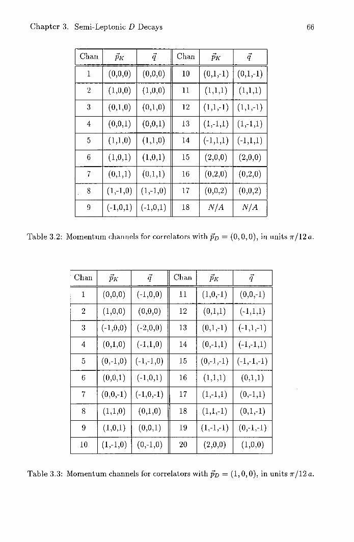
Chapter 3. Semi-Leptonic D Decays
Ell
Chan P-K Chan I PK
1 (0,0,0) (0,0,0) 10 (0,1 ) - i) (0,1 )- i)
2 (1,0,0) (1,0,0) ii (1,1,1) (1,1,1)
3 (0,1,0) (0,1,0) 12
4 (0,0,1) (0,0,1) 13 (i,-i ) i)
5 (1,1,0) (1,1,0) 14
6 (1,0,1) (1,0,1) 15 (2,0,0) (2,0,0)
7 (0,1,1) (0,1,1) 16 (0,2,0) (0,2,0)
8 (1 )-1 1 0) (1 )-1 10) 17 (0,0,2) (0,0 ) 2)
9 (-1,0,1) (-1,0,1) 18 N/A N/A
Table 3.2: Momentum channels for correlators with P-D = (0, 0, 0), in units 702 a.
Chan] 13K Chan PK
i (0,0,0) (-1,0,0) ii (1,0,-1) (0,0,-1)
2 (1,0,0) (0,0,0) 12 (0,1,1) (-i,i,i)
3 (-1,0,0) (-2,0,0) 13 (0,1 1-1)
4 (0,1,0) (-1,1,0) 14 (0 1-1 1 1)
5 (0 1-1,0) (-1,-1,0) 15 (0,-1,-1)
6 (0,0,1) (-1,0,1) 16 (i,i,i) (0,1,1)
7 (0,0,-1) (-1,0,-1) 17 (i,-i,1) (0,-1,1)
8 (1,1,0) (0,1,0) 18 (1,1 )-1) (0,1,-i)
9 (1,0,1) (0,0,1) 19 (i,-i,-1) (0 )-i,-i)
10 (1 )-1,0) (0,-1,0) 20 (2,0,0) (1,0,0)
Table 3.3: Momentum channels for correlators with pj = (1, 0, 0), in units 7r/12 a.

Chapter 3. Semi-Leptonic D Decays
67
Three-Point Correlator Data
Three-point correlators were computed for a fixed charm quark mass with hopping
parameter r1h = 0.129; for two values of the strange quark mass with ic = 0.14144
and 0.14226; and for three values of the light quark mass with 'c j = 0.14144,
0.14226, and 0.14262. These hopping parameter values correspond to six kappa-
independent three-point correlators.
For each kappa combination, the correlator data consists of 2220 (37 momentum
x 60 Lorentz) channels per timeslice. To reduce storage overheads only timeslices
t = 7-16 and t = 32-41 are saved; these intervals corresponds to the 'forward'
and 'backward' correlator components respectively which are well separated in
Euclidean time. Prior to fitting, the configuration data is folded by averaging the
corresponding timeslices from the two halves of the lattice.
To increase statistics, the correlator data is averaged over all equivalent
momentum channels; and over all Lorentz channels corresponding to the same
matrix element. For example, when pjj = (0, 0, 0) the momentum channels with
PK(*) = (1,0,0), (0,1,0) and (0,0,1), in units of 7r/12 a, are equivalent and their
average corresponds to a decay with momentum transfer I fl = 7r/12 a.
The D -+ K, K* form factors are obtained by performing simultaneous fits to all
Lorentz-independent three-point correlators. The energies and the corresponding
two-point amplitudes in Eqns. (3.38)-(3.41) are constrained to the values obtained
from two-point correlator fits, as detailed in Chapter 2. In the following section,
the 'time-independent' correlators are defined as three-point correlators with these
two-point factors removed. Thus, each Lorentz-independent correlator component
is fitted (simultaneously) to a constant or 'plateau'. The masses and energies
corresponding to the form factor parameterisation are also constrained to values
obtained from two-point correlator fits.
Correlated chi-squared fits are performed but only correlations between timeslices
corresponding to the same matrix element are kept since different matrix elements
may have different systematic errors. For each correlator component, the fit in-
terval is t=11-13; for t=12 the weak current operator is equidistant from both
the D and K(*) mesons.

Chapter 3. Semi-Leptonic D Decays
Pseudoscalar-to-Pseudoscalar Fits
For each momentum channel, the form factors f+ and f 0 are obtained by perform-
ing a simultaneous fit to all Lorentz-independent pseudoscalar-to-pseudoscalar
three-point correlators. Using the (second) form factor parameterisation, given
by Eqn. (3.11), the time-independent correlators can be written as follows:
Zv x (K 1 70 1 D) = (ED + EK) f + (ED — EK) f (3.43)
zv X(KD) = (PD +pK)f+ (pD - pK)f (3.44)
where (K 1 70 1 D) and (K D) denote the temporal and spatial correlator
components respectively, and Zv is the renormalisation constant corresponding
to the lattice vector current. Thus, in general there are (at least) two Lorentz-
independent pseudoscalar-to-pseudoscalar three-point correlators.
However, for the momentum channel (0, 0, 0) —+ (0, 0, 0) there is only one non-zero
component. Using the (first) form factor parameterisation, given by Eqn. (3.1),
the temporal component is given by
Zv x (K -y o D)= (MD + MK) f° (3.45)
where the momentum of both the D and K mesons is zero. Thus, for this channel
the form factor f 0 is obtained from a one-parameter fit; there is no determination
of the form factor f+. For the momentum channel (1,0,0) —+ (0, 1, 0) there are
three Lorentz-independent correlator components: one temporal and two spatial.
Thus, the form factors f+ and f0 are obtained from a two-parameter fit which is
over-determined.
The form factors f+ and f°, obtained from simultaneous fits to pseudoscalar-to-
pseudoscalar correlators, are given in Table 3.4 with the corresponding q 2 values
computed from the meson masses, given in Tables 2.1 and 2.3. In general, the chi-
squared values indicate a good fit to the data for all kappa combinations. However,
for the channel (1, 0,0) -+ (-1,0,0) the fit chi-squared are on the high side which
suggests that one of the correlator components has not plateaued within the fit
window.

Chapter 3. Semi-Leptonic D Decays
ME
PD I'K KI ici. a 2 q2 f + /zv x 2 /dof
(0,0,0) (0,0,0) 0.14144 0.14144 0.175 i N/A 0.8 1.03 ii
0.14226 0.209 N/A 1.5 0.99 t
0.14226 0.14144 0.188 ii N/A 1.1 1.04
0.14226 0.229 ii N/A 1.9 1.00
0.14262 0.14144 0.195 t N/A 0.8 1.05
0.14226 0.241 ji N/A 1.6 1.02 ii
(0,0,0) (1,0,0) 0.14144 0.14144 0.034 it 0.91 it 0.7 0.87 it 0.14226 0.053 it 0.88 it 0.8 0.81 it
0.14226 0.14144 0.037 0.90 0.6 - 0.85
0.14226 0.057 it 0.86 it 0.7 0.78 it
0.14262 0.14144 0.038 it 0.88 it 0.5 0.83 it
0.14226 0.060 + 3 0.84 ii 0.6 0.75 it
(1,0,0) (0,0,0) 0.14144 0.14144 0.147 t 1.25 it 1.2 0.98 it 0.14226 0.185 it 1.33 + 10 1.1 0.96
0.14226 0.14144 0.163 it 1.27 it 0.6 0.99 it
0.14226 0.208 it 1.40 it 0.2 1.00
0.14262 0.14144 0.172+ 1.26 it O.9 0.99 it
0.14226 0.222 i 1.42 it 0.5 1.01 it
Table 3.4: The D -* K form factors with momentum in units of 7r/12a and kh = 0.129.

Chapter 3. Semi-Leptonic D Decays
70
PD I PK 'ci a2 q2 f/Zv x 2 /dof I f 0/
Zv (1,0,0) (1,0,0) 0.14144 0.14144 0.134 it 1.13 + 9 0.1 0.91 it
0.14226 0.155 it 1.12 it ' 0.3 0.82 it
0.14226 0.14144 0.138 it 1.08 0.6 0.78 it 14
0.14226 0.162 it 1.07 it 0.6 0.64
0.14262 0.14144 0.141 + 3 0.99 it 1.0 0.59 it 0.14226 0.165 + 4 0.94 it 0.8 0.41 ii
(1,0,0) (-1,0,0) 0.14144 0.14144 -0.140+ 0.60 2.2 0.72 it 0.14226 _0.119+ 0.58 1.8 0.69 it
0.14226 0.14144 -0.136 it 0.60 it 3.4 0.71 it 0.14226 -0.113 + 3 0.59 it 2.8 0.69 it
0.14262 0.14144 -0.133+ 0.58 it 3.8 0.70 ii 0.14226 -0.109 it 0.58+ 70 3.5
(1,0,0) (0,1,0) 0.14144 0.14144 -0.003 it 0.78 it 1.2 0.78
0.14226 0.018 it 0.75 it 1.1 0.73 it
0.14226 0.14144 0.001 it 0.76 it 0.5 0.76 it 0.14226 0.025 it 0.73 it 0.3 0.70
0.14262 0.14144 0.004 074+ 6 0.2 0.74
0.14226 0.028 it 0.71 it 0.1 0.68
Table 3.4: (Cont.)

Chapter 3. Semi-Leptonic D Decays 71
1.4
1.2
1.0
0.8
0.6
I- Pseudo : p(O,O,O)-'p(O,O,O) 1.0
0.8
1L1
0.4
Pseudo : p(O,O,O)-p(l,O,O)
0 10 20 Fit Range = [11, 13], X2/dof = 1.5 / 2
Pseudo : p(l,O,O)-p(O,O,O) 1.0
0.5
0.0 r I I I I I I 0 10 20 30 40 Fit Range = [11, 131, X2/dof = 4.9 / 4
II III 111 1 11 11 1 111 l i ii
- Pseudo : p(l,O,O)-p(-1,O,O)
0 10 20 30 40 Fit Range = [11, 13], X2/dof = 2.7 / 4
1.4 I I I Pseudo : p(l,O,O)-p(l,O,O)
:: •
0.8— -
06—
0.4
I I I I I I I I I I I I I I I I I I I I
0 10 20 30 40 Fit Range = [11, 13], X2/dof = 0.48 / 4
1.0
- Pseudo : p(1,0,0)p<O,1,0>
FIIGI
0.5
NERIXII
on
0 10 20 30 40 0 20 40 60 Fit Range = [11, 131, X2/dof = 9 / 4 Fit Range = [11, 13], X2/dof = 6.3 / 7
Figure 3.2: Pseudoscalar-to-Pseudoscalar plateau plots with ic = 0.14144 and 'h = 0.129. Momentum in units of 7r/12 a.

Chapter 3. Semi-Leptonic D Decays 72
Figure 3.2 shows six 'plateau' plots, one for each momentum channel, corre-
sponding to the simultaneous fit of Eqns. (3.43) and (3.44) to the temporal
and spatial correlator components respectively. The plateau plot shows each
Lorentz-Independent component fitted (simultaneously) to a constant; the time-
dependence has been removed by multiplying by the appropriate two-point factor.
These plots serve as a guide to the 'quality' of the plateau in the three-point data.
Vector-to-Pseudoscalar Vector Fits
For each momentum channel, the vector form factor is obtained by performing a
simultaneous fit to all Lorentz-independent three-point correlators. Multiplying
both sides of Eqn. (3.2) by a 'dummy' polarisation vector, summing over polar-
isation states of the vector K* meson, and using the polarisation sum identity,
given in Eqn. (1.107), one obtains the form factor parameterisation corresponding
to the polarisation-averaged vector three-point correlator:
Zv x '3)
x (3.46) 2V
= m*
—g M + mK*
with
(KVD) (3.47)
where VI" is the time-independent three-point correlator data, and Zv is the
renormalisation constant corresponding to the lattice vector current.
The form factor V, obtained from simultaneous fits to vector-to-pseudoscalar
vector correlators, is given in Table 3.5 with the corresponding q 2 values computed
from the meson masses, given in Tables 2.1 and 2.3. For the momentum channel
(0, 0, 0) -+ (0, 0, 0) all Lorentz components are zero and there is no determina-
tion of the vector form factor. In general, there is only one Lorentz-independent
component and V is obtained from a one-parameter fit. However, for the momen-
tum channel (1,0,0) -+ (0, 1,0) there are three Lorentz-independent correlators: a
mixed temporal and spatial component, and two spatial components correspond-
ing to the longitudinal and transverse contributions with respect to the momentum
of the D meson. Thus, for this channel V is obtained from a one-parameter fit
which is over-determined.

Chapter 3. Semi-Leptonic D Decays 73
PD PK ici IcE. a 2 q 2 V/Zv x 2 /dof
(0,0,0) (0,0,0) 0.14144 0.14144 0.103+ 3 N/A N/A
0.14226 0.120 ji N/A N/A
0.14226 0.14144 0.104ji N/A N/A
0.14226 0.122 ji N/A N/A
0.14262 0.14144 0.104 i!i N/A N/A
0.14226 0.124 t N/A N/A
(0,0,0) (1,0,0) 0.14144 0.14144 -0.010 t 1.49 0.17
0.14226 0.000 i 1.47 + 10 0.55
0.14226 0.14144 -0.012+ 1.45 ' 0.74
0.14226 -0.001 t 1.41 t 1.94
0.14262 0.14144 -0.012 i 1.43 j 0.96
0.14226 -0.001 ii 1.36 ii 1.69
(1,0,0) (0,0,0) 0.14144 0.14144 0.067 1.46+ i 0.01
0.14226 0.085 t 1.38 t 0.30
0.14226 0.14144 0.068+ 1.35 16 0.20
0.14226 0.089 i 1.28 ii 0.32
0.14262 0.14144 0.069 1.40 30 0.38
0.14226 0.092+ 9 i 1.39 0.37
Table 3.5: The D -p K* vector form factor with momentum in units of 7r/12 a and Ich = 0.129.

Chapter 3. Semi-Leptonic D Decays
74
PD PK tci Ki. a2 q2 V/Zv I x2/dof
(1,0,0) (1,0,0) 0.14144 0.14144 0.083 t 2.7 ii 0.71
0.14226 0.096 ii 3.0 t 1.33
0.14226 0.14144 0.082 3.4 t 3.15
0.14226 0.095 t 4.1 + 10 6.35
0.14262 0.14144 0.082 i 3.7 it 5.65
0.14226 0.096 + 6 5.2 8.75
(1,0,0) (-1,0,0) 0.14144 0.14144 -0.191 ii 0.90 0.08
0.14226 -0.179 it 0.90 + 11 0.06
0.14226 0.14144 -0.192 it 0.85 it 0.04
0.14226 -0.179 + 4 0.87 it 0.01
0.14262 0.14144 -0.192 !i 0.80 0.02
0.14226 -0.179 0.81 25 0.07
(1,0,0) (0,1,0) 0.14144 0.14144 -0.054 it 1.22 it 1.15
0.14226 -0.042 +3 1.18 1.18 10 1.40
0.14226 0.14144 -0.055 i 1.11 ii 1.20
0.14226 -0.042 ii 1.06 i 1.38
0.14262 0.14144 -0.055 ii 1.00 it 1.19
0.14226 -0.042 ii 0.90 it 1.18
Table 3.5: (Cont.)

Chapter 3. Semi-Leptonic D Decays
75
0.6
Vector p(0,0,0)-p(1,0,0)
Vector p(l,O,O)-*p(O,O,O)
—0.2
[.LI
I1wI
0.411111 11 1 1 1 1 1
0 10 20 Fit Range = [11, 131, X2/dof = 0.34 / 2
0.6
I I I I I I I I I II
0 10 20 Fit Range = [11, 131, X 2/dof = 0.012 / 2
Vector : p(1,0,0)-p(1,0,0)
0.4
0.2
fin
0 10 20 Fit Range = [11, 13], X2/dof = 1.4 / 2
—0.4
- Vector : p(1,0,0)p(-1,0,0)
- Vector : p(1,0,0)p<0,1,0>
0.5
=ii;i
0.0
0.71 I I I I I I I I
I1111111 I I I I I I I I II
0 10 20 0 20 40 60 Fit Range = [11, 13], X2/dof = 0.17 / 2 Fit Range = [11, 13], X2/dof = 9.2 / 8
Figure 3.3: Vector-to-pseudoscalar vector plateau plots with rj - = 0.14144 and ilch = 0.129. Momentum in units of 7r/.12 a.

Chapter 3. Semi-Leptonic D Decays 76
In general, the chi-squared values quoted in Table 3.5 indicate a good fit to the
correlator data for all kappa combinations. However, for the momentum channel
(1, 0, 0) -+ (1, 0,0) the fit chi-squared are on the high side which suggests that
the time-independent correlator data is not plateauing within the fit window.
Figure 3.3 shows six plateau plots, one for each momentum channel, corresponding
to the simultaneous fit of Eqn. (3.46) to the Lorentz-independent vector-to-pseudo-
scalar vector correlator components.
Vector-to-Pseudoscalar Axial Fits
For each momentum channel, the axial form factors are obtained by performing
a simultaneous fit to all Lorentz-independent vector-to-pseudoscalar three-point
correlators. Multiplying both sides of Eqn. (3.2) by a 'dummy' polarisation vector
one obtains the form factor parameterisation corresponding to the polarisation-
averaged axial three-point correlator:
_ / PDPK
ZA x A = (g - ) (m + MK-) A 1 - (PD - 2 PK*) M 2
f A2 (PD +PK*Y - 2AmK* (PD _PK*Y } (3.48)
q2
with
AIL' = (KAD)
(3.49)
where AV is the time-independent three-point correlator data, and ZA is the
renormalisation constant corresponding to the lattice axial current.
The form factors A 1 , A 2 and A° , obtained from simultaneous fits to vector-to-
pseudoscalar axial correlators, are given in Table 3.6 with the corresponding q2 values given in Table 3.5. For the momentum channel (0, 0, 0) -* (0, 0, 0) the form
factor parameterisation, given by Eqn. (3.48), reduces as follows:
ZA x A 23 = - (MD +mK*)A1; i=i (3.50)
A 23 = 0; i j (3.51)
where the temporal component A °° is zero. Thus, the form factor A 1 is obtained
from a one-parameter fit; there is no determination of the form factors A 2 and A0.

Chapter 3. Semi-Leptonic D Decays
77
PD PK KI 'ci8 A'/ZA A 2 /ZA A ° /ZA x2 /dof
(0,0,0) (0,0,0) 0.14144 0.14144 0.74 t N/A N/A 2.0
0.14226 0.70 j N/A N/A 1.6
0.14226 0.14144 0.76 i N/A N/A 0.9
0.14226 0.72 N/A N/A 0.5
0.14262 0.14144 0.78 j N/A N/A 0.6
0.14226 0.73 i N/A N/A 0.2
(0,0,0) (1,0,0) 0.14144 0.14144 0.70 t 0.59 i 0.73 ii 1.2
0.14226 0.65 i!i 0.51 it 0.72 it 0.6
0.14226 0.14144 0.71 j 0.62 0.73 it 0.8
0.14226 0.66 it 0.53 it 0.72 0.6
0.14262 0.14144 0.71 it 0.61 0.73 t 0.8
0.14226 0.64 t 0.50 0.72 ii 0.8
(1,0,0) (0,0,0) 0.14144 0.14144 0.69+ 0.66 0.88 1.0
0.14226 0.66 ii 0.93 0.88 it 0.8
0.14226 0.14144 0.69 i
i
i 0.58 ii 0.92 ii 0.9
9
1 0.14226 0.65 t 0.92t 0.8
0.14262 0.14144 0.69 ii 0.39 it 0.98 ji 0.6
0.14226 0.65+ 0.75 + 121 - 90 1.00 0.6
Table 3.6: The D -+ K* axial form factors with momentum in units of 7r/12 a; the corresponding q2 values are given in Table 3.5.

Chapter 3. Semi-Leptonic D Decays in
PD I PK A 1 1ZA I A 2 /ZA A ° /ZA x 2 /dof
(1,0,0) (1,0,0) 0.14144 0.14144 0.75 i 6 1 4 + 12 -11 0.93+ 13
-11 0.6
0.14226 0.71 + 7
13 1. 4 +-12 -' 96 + 18 -14 0.8
0.14226 0.14144 ' 65 + 15 '-'S -13 0.6 + 19
-20 0.75 + 23 -20 0.9
0.14226 0.59 +'8 0.6 iT 0.78 iT 1.0
0.14262 0.14144 0.49+ 24 21 -0.7 + 30
-29 0.53 iT 1.1
0.14226 0.41 +30 -0.9 + 32 31 0.57 + 41
-42 1.0
(1,0,0) (-1,0,0) 0.14144 0.14144 0.57 0.36 i 0.44 1.4
0.14226 0.53 iT 0.30 + 10 0.44 t 1.1
0.14226 0.14144 0.59 iT 7 0 37 + 14 -12 0.45 ii 1.0
0.14226 0.56 -F 10 9 0.31 + 17
-15 0.47 0.7
0.14262 0.14144 0.58 + 14 - 12 0.34 + 20
. - 20 0.46 0.8
0.14226 058+ 15 030+ 24 050 - -o 0.6 -16 . -24
(1,0,0) (0,1,0) 0.14144 0.14144 0.61 ii 0.41 0.62 1.4
0.14226 0.56 iT 0.35 IT 0.60 1.1
0.14226 0.14144 0.59 iT 0.35 iT 0.63 iT 1.3
0.14226 0.53 -F 6 4 0.29 + 14
-13 0.60 iT 1.0
0.14262 0.14144 0.54 iT 8 6 0.23 + 20
-16 0.63 iT 1.3
0.14226 0.48 +'o 0.19 iT 0.61 + 10 1.0
Table 3.6: (Cont.)

Chapter 3. Semi-Leptonic D Decays
79
0.0
Axial :
—0.5
—1.0
—1.5 11 1 1 1 1 1
0 10 20 Fit Range = [11, 13], X2/dof = 4 / 2
Axial : p(l,O,O)-*p(O,O,O)
- 1 . 0 . I III
0 20 40 60 Fit Range = [11, 131, X2/dof = 5.7 / 6
Axial : p(i,o,o)-+p(—i,o,o)
u.0 I I I I I I I Axial : p(0,0,0)-p(1,0,0)
0 50 100 Fit Range = [11, 131, X2/dof = 14 / 12
0.0
Axial : p(l,O,O)-*p(l,O,O)
'11
—1.0
_1.51 I I I I I
0 50 100 Fit Range = [11, 13], X2/dof = 6.9 / 12
Axial : p(1,0,0)-p<0,1,0>
0.0
IK•I
—0.5
0.5
0.0
—0.5
—0.5
_1.0I I I I I I I I I _1.0I I I I I I I I I I I
0 50 100 0 100 200 Fit Range = [11, 13], X 2/dof = 16 / 12 Fit Range = [ii, 13], X 2/dof = 37 / 27
Figure 3.4: Vector-to-pseudoscalar axial plateau plots with rl = nl,, = 0.14144 and
Kh = 0.129. Momentum in units of 7r /12 a.

Chapter 3. Semi-Leptonic D Decays 80
In general, there are three or more Lorentz-independent correlators and the form
factors A', A 2 and A 0 are obtained from a three-parameter fit which (in most
cases) is over-determined. The chi-squared values, quoted in Table 3.6 indicate
a good fit to the data for all kappa combinations. Figure 3.4 shows six plateau
plots, one for each momentum channel, corresponding to the simultaneous fit
of Eqn. (3.48) to the Lorentz-independent vector-to-pseudoscalar axial correlator
components.
3.4 Form Factor Extrapolations
Recall from Section 3.3, the form factors describing the D -+ K, K* decays were
obtained from simultaneous fits to three-point correlators computed for six kappa
combinations. In this section, the form factors are extrapolated to the physical
quark masses: the strange and light quark masses, determined in Section 2.4, cor-
responding to K, = 0.1418 i and tt = 0.14315 !i respectively. The form factors
describing the related decays D -+ ir, p are also computed.
Form Factor Mass Dependence
Recall from Section 3.1, in the pole dominance model the q2 dependence of the
form factors is given by
F(q2) = _° 2 (3.52) q
where F is a generic form factor and mp ol e is the mass of the corresponding
resonance. In this study, the form factors are assumed to have the following
dependence on the light quark masses:
LmD(Kl) LmK() ('cia, ') (ic1 5 , Icl)'\+d
2
mD(k) mK(*)(IcS,IcC) ( AMK(-)
mK(.)(IcS,lcC) ) ( 3.53) F(ic1 , dcl) = a + b +c
with AMD(Ic1) and /mK(*)(Icj,!c1) defined as follows:
LmD(Icl) = mD(Il) - mD(Ic) (3.54)
LrflK(.) (Ici, 'ci) = rnK(.) (a'cl, ti) - mK(*) ('ce, (3.55)
where MD (r.1) is given by Eqn. (2.27), and mK(lc1,Ic1) and MK* (1c1 3 ,Icl) are given
by Eqns. (2.20) and (2.23) respectively.
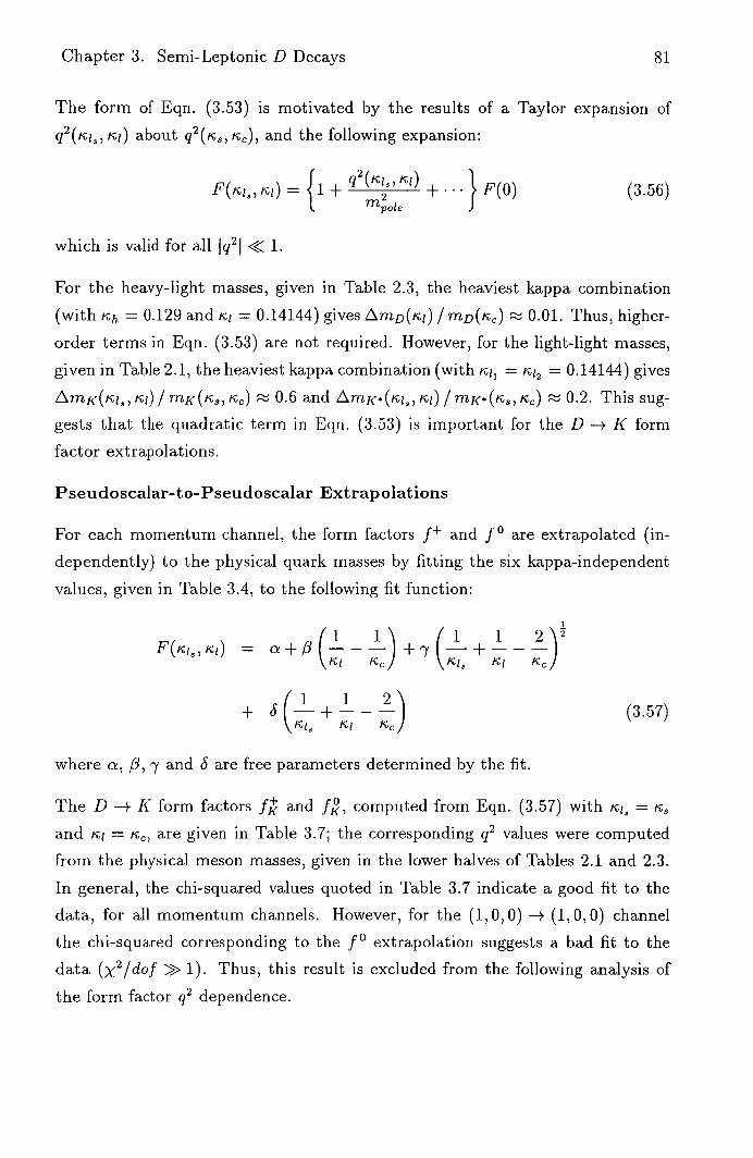
Chapter 3. Semi-Leptonic D Decays 81
The form of Eqn. (3.53) is motivated by the results of a Taylor expansion of
q2 (,c, 'ci) about q2 (i'c 8 , ,c), and the following expansion:
+ q2(k18,1)
+ . .. } F(0) (3.56) 2
m 0 1
which is valid for all 1q 2 1 << 1.
For the heavy-light masses, given in Table 2.3, the heaviest kappa combination
(with kh = 0.129 and 'ci = 0.14144) gives LmD(!cl) / mi(ic) 0.01. Thus, higher-
order terms in Eqn. (3.53) are not required. However, for the light-light masses,
given in Table 2. 1, the heaviest kappa combination (with ice, = ic12 =0.14144) gives
LmK('cl 8 ,'cl)/rnK(/c3,IcC) 0.6 and LmK('c1 3 ,/cj)/ MK- (Ic,Ic) 0.2. This sug-
gests that the quadratic term in Eqn. (3.53) is important for the D —4 K form
factor extrapolations.
Pseudoscalar-to-Pseudoscalar Extrapolations
For each momentum channel, the form factors f+ and f0 are extrapolated (in-
dependently) to the physical quark masses by fitting the six kappa-independent
values, given in Table 3.4, to the following fit function:
1 1fi 1 2 2
a+ --- +(—+--- - (KI ) \'ci.
(I 2 + 8 + ' (3.57) --
\. 'i8 it ice) -1
where a, /, 'y and 8 are free parameters determined by the fit.
The D —+ K form factors f and f, computed from Eqn. (3.57) with ic =
and 'i = ,c, are given in Table 3.7; the corresponding q2 values were computed
from the physical meson masses, given in the lower halves of Tables 2.1 and 2.3.
In general, the chi-squared values quoted in Table 3.7 indicate a good fit to the
data, for all momentum channels. However, for the (1,0,0) –+ (1, 0,0) channel
the chi-squared corresponding to the f° extrapolation suggests a bad fit to the
data (x 2 /dof >> 1). Thus, this result is excluded from the following analysis of
the form factor q2 dependence.

Chapter 3. Semi-Leptonic D Decays
PD PK a2 q2 f/Zv I X2/dof fi _f)/Zv I x2/dof
(0,0,0) (0,0,0) 0.230 t N/A N/A 1.04 t 0.43
(0,0,0) (1,0,0) 0.050 0.86 i 0.52 0.77 ii 0.92
(1,0,0) (0,0,0) 0.212 1.41 0.32 1.03 0.14
(1,0,0) (1,0,0) 0.156 i 1.16 1.40 0.77 t 2.82
(1,0,0) (-1,0,0) -0.119 0.62 t 0.13 0.73 O 0.09
(1,0 1 0) (0,1,0) 0.018 + + it 0.24 0.72 t 0.24
Table 3.7: The D -* K form factors with momentum in units of 7r/12 a.
PD PK a 2 q 2 f7/Zv
(0,0,0) (0,0,0) 0.380 t N/A 1.00 + 31 - 12
(0,0,0) (1,0,0) 0.091 0.76 it 0.56 + 14 -8
(1,0,0) (0,0,0) 0.375 i 3 2 + 36 - 1.25 + 18 - 20
(1,0,0) (1,0,0) 0.202 ii 1.30 0.11 + 47 - 32
(1,0,0) (-1,0,0) -0.073 t 0.73 ii 0.84 + 31 - 20
(1,0,0) (0,1, 0) 0.065 0.72 it 0.61 + 15 - 13
Table 3.8: The D -+ it form factors with momentum in units of 7r/12 a; the fit chi-squared are the same as those in Table 3.7.

Chapter 3. Semi-Leptonic D Decays
1.0 1.0
- Extrap f (0,0,0(1,0,0)
0.9
0.9
+ + •1-
0.8
0.8
X2/dof = 1.04 / 2
7.00 7.05 7.10
1 / c 1
Extrap f : (0,0,0)-+(1,0,0)
±cy H
X2/dof = 1.44 / 3
7.00 7.05 7.10
1 / ic 1
>. 1.4
+ 4-.
1.2
1.0
Extrap f (1,0,0)-+(0,0,0)
- X2/dof = 0.64 / 2
. 1.4
+
1.2
Extrap f : (1,0,0)(0,0,0) -
I - X2/dof = 3.41 / 3
7.00 7.05 7.10
7.00 7.05 7.10
1 / ,c 1 1 /
0.7
... 0.6 + 4-.
0.5
Extrap f : ( 1,0,0)-*(-1,0,0)
ft X2/dof = 0.26 / 2 -
0.7
- 0.6 + 4-.
0.5
Extrap f : (1,0,0)-+(-1,0,0)
X2/dof = 1.23 / 3
Figure 3.5: Extrapolation plots for the f form factor.

Chapter 3. Semi-Leptonic D Decays 84
Recall from Section 2.4, the lattice pion mass computed using Eqn. (2.20) with
nil = K12 = r c is zero by definition. However, in order to compute the D —+ it
form factors, and the corresponding q2 values, a non-zero estimate of the light
quark mass is required. Fixing the light-light pseudoscalar mass mp = 0.05 in
Eqn. (2.20) gives
ic1 = kd = 0.14310 (3.58)
which corresponds to a physical pion mass with m, 140 MeV. In practice, the
use of massless u and d quarks has no effect on the determination of ic 3 , or m which
is used to set the lattice spacing. The D -* IV form factors f and f,°, computed
from Eqn. (3.57) with 'ci, =ni =nu ,are given in Table 3.8; the corresponding q2
values were computed using m,r = 0.05 and the physical D meson mass, given in
the lower-half of Table 2.3.
Figure 3.5 shows the f form factor data, given in Table 3.4, plotted as a function
of the inverse light-kappa, 'ci, for three different momentum channels. This data,
denoted by 'circles', is fitted to Eqn. (3.57) as follows: the left-hand plots corre-
spond to four-parameter fits; the right-hand plots correspond to three-parameter
fits with the S parameter constrained to zero. The 'diamonds' correspond to the
form factor f+ computed using Eqn. (3.57), for each of the six kappa combina-
tions; the extrapolated form factor f is denoted by a cross. Note, the data lies
in two distinct planes which correspond to the two values of the strange kappa,
For small 8, the f form factor will lie on a plane bisecting these two data
planes.
The 'extrapolation' plot gives an indication of how well the fit function is modelling
the data: a good fit function will reproduce the data, i.e. the circles and diamonds
will overlap. From Figure 3.5 it is clear that the quadratic term in Eqn. (3.57) is
important: for the momentum channel (1, 0, 0) —+ (0, 0,0) the extrapolated results
differ by as much as 15% between the two fit methods. In general, the four-
parameter fit gives a smaller chi-squared and the corresponding extrapolation
plot has a better 'overlap'. However, this method gives slightly larger errors on
the extrapolated form factor. The D —+ K and D -+ iv form factors quoted in
Tables 3.7 and 3.8 were obtained using the four-parameter fit method.

Chapter 3. Semi-Leptonic D Decays 85
PD I PK 11 a 2 q 2 VK*/ZV x 2 /dof
(0,0,0) (0,0,0) 0.112 i N/A N/A
(0,0,0) (1,0,0) -0.009+ 1.4 it 0.12
(1,0,0) (0,0,0) 0.079 + 9 1.0 t 0.76
(1,0,0) (1,0,0) 0.086 3.8 1.85
(1,0,0) (-1,0,0) -0.188 0.8 0.37
(1,0,0) (0,1,0) -0.051 ii 1.1 it 0.61
Table 3.9: The D -* KK vector form factor with momentum in units of 7r/12 a.
PD PK a 2 q 2 V/Zv
(0,0,0) (0,0,0) 0.142 + 9 NIA
(0,0,0) (1,0,0) 0.007 +' 1.4
(1,0,0) (0,0,0) 0.113 1.0 it
(1,0,0) (1,0,0) 0.106 it 4.0 it 15
(1,0,0) (-1,0,0) -0.168 it 6 6 0.8 it
(1,0,0) (0,1,0) -0.031 it 1.0 t
Table 3.10: The D -+ p vector form factor with momentum in units of ir/12 a; the fit chi-squared are the same as those in Table 3.9.

Chapter 3. Semi-Leptonic D Decays
MI
[_PD 73K Ak*/ZA x 2 /dof A*/ZA x 2 /dof _A < ./ZA x 2 /dof
(0,0,0) (0,0,0) 0.76 it 0.25 N/A N/A N/A N/A
(0,0,0) (1,0,0) 0.71 it 0.17 0.7 it 0.11 0.72 0.09
(1,0,0) (0,0,0) 0.67 it 0.03 0.5 0.15 0.92 it 0.26
(1,0,0) (1,0,0) 0.68 +17 0.61 1.4 - 27 0.38 0.75 j 0.41
(1 0,0) (-1,0,0) 0.59 it 12 0.44 0.4 0.21 0.44 ii 0.69
(1,0,0) (0,1,0) 0.58 it 0.84 0.4 it 0.63 0.59 ii 0.16
Table 3.11: The D -+ K* axial form factors with momentum in units 702 a. The corresponding q 2 values are given in Table 3.9.
PD 73K A/ZA A/ZA A/ZA
(0,0,0) (0,0,0) 0.69+ 8 NIA N/A
(0,0,0) (1,0,0) 0.64 it 0.5 it 0.71 it
(1,0,0) (0,0 ) 0) 0.61 + 9 0.9 it 0.90 it 18
11 , n , n\ (1 n r) 19 0.62 +18 1r + 29
- 28 81 +43
23
i
(1,0,0) (-1,0,0) 0.52 t " i
-
050 i
0.3 t 0.43 t
(1,0,0) (0,1,0) . 03 t 0.56
Table 3.12: The D -* p axial form factors with momentum in units 7r/12 a; the fit chi-squared are the same as those in Table 3.11. The corresponding q 2 values are given in Table 3.10.

Chapter 3. Semi-Leptonic D Decays
Extrap V : (0,0,0)-*(1,0,0) -
1.4
1.2
- X2/dof = 0.37 / 3
u.o
- Extrap A 1 (0,0,0)(1,0,0) -
0.7
0.6
X2/dof = 0.52 / 3
7.00 7.05 7. 7.00 7.05 7.
1 / ,c 1 1 / ,c 1
0.8
2.0
1.5
1.0
Extrap V : (1,0,0)-*(0,0,0)
I X2/dof = 2.29 / 3
Extrap A 1 : ( 1,0,0)(0,0,0)
0.7
0 Ow
0.6
- X2/dof = 0.09 / 3
1.2
1.0
-. 0.8
0.6
0,4
7.00 7.05 7.
1 / ,c
Extrap V (1,0,0)-(-1,0,0)
X2/dof = 1.10 / 3
0
0.8
. 0.6 NJ
0.4
7.00 7.05 7.
1 / ,c
- ExtrapA 1 :(1,0,0)-(-1,0,0)
X2/dof = 1.30 / 3
Figure 3.6: Extrapolation plots for the V and A 1 form factors.

Chapter 3. Semi-Leptonic D Decays
Pseudoscalar-to-Vector Extrapolations
For each momentum channel, the vector and axial form factors are extrapolated
(independently) to the physical quark masses by fitting the six kappa-independent
values, given in Tables 3.5 and 3.6 respectively, to the following fit function:
I
1 1 fi 1 2 2
( )
F(ici3 , 'ci) = a + /9 - - - + -Y + - - - (3.59)
where a, 3, and 'y are free parameters determined by the fit.
The D —* K* vector and axial form factors, computed from Eqn. (3.59) with ic =
ic and KI = ic e , are given in Tables 3.9 and 3.11 respectively; the corresponding q2
values were computed from the physical meson masses, given in the lower halves
of Tables 2.1 and 2.3. In general, the chi-squared values indicate a good fit to the
data, for all momentum channels. However, for the (1,0,0) (1,0,0) channel the
chi-squared corresponding to the V extrapolation (x 2 /dof = 1.85) suggests a bad
fit to the data. Similarly, a large error on A 2 corresponds to a poor determination
of the form factor for this momentum channel. Thus, these results are excluded
from the following analysis of the form factor q 2 dependence.
The D -+ p form factors were also computed: the vector and axial form factors,
computed from Eqn. (3.59) with Icj, = KI = are given in Tables 3.10 and 3.12
respectively. Figure 3.6 shows extrapolation plots for three different momentum
channels: the left-hand and right-hand plots correspond to the V and A 1 form
factor data, given in Tables 3.5 and 3.6 respectively, fitted to Eqn. (3.59). In
general, the three-parameter fit gives an excellent description of the data. Thus,
additional (quadratic) terms in Eqn. (3.59) are not required.
3.5 Pole Dominance Fits
In Section 3.4, the D -+ K, K* and D —+ rr, p form factors were extrapolated to
their physical values, for a range of q2 . This data could be used to test the pole
dominance relations, given by Eqns. (3.15)—(3.17), from first principles. The q2
dependence of the form factors is required to determine the decay rates. However,
the scalar (0+) and axial (1+) pole masses are poorly determined. Thus, in this
Section, the form factor data is fitted to the pole dominance model.

Chapter 3. Semi-Leptonic D Decays
FIN
Pseudoscalar-to-Pseudoscalar Form Factors
Figures 3.7 and 3.9 show the fK and f form factor data, given in Tables 3.7
and 3.8 respectively, plotted as a function of q2 . The f and f data is fitted
to the pole dominance model, given by Eqn. (3.52), as follows: the left-hand
plots correspond to a two-parameter fit; the right-hand plots correspond to a
one-parameter fit with the pole mass constrained to the mass of the associated
resonance, MD- and MD. respectively. In the pole dominance plot, the solid 'fit'
line corresponds to the kinematically allowed region, given by Eqn. (3.4), and the
'cross' denotes the extrapolated form factor, F(0).
For the f data the two fit methods give a consistent determination of f(0); the
two-parameter fit yields
f(0) - c
0.76 + ; m 1 _ = 0.68 + (3.60) zv -
where the pole mass agrees (within errors) with both the lattice value 0.736 i ,
given in Table 2.3, and with the experimental value 2.00 ii 0.12 ii 0.18 GeV, quoted
in Section 3.2. The chi-squared (x2/dof = 0.37) indicates an excellent fit to the
data; all data points lie within one sigma, for both fit methods. Thus, pole
dominance gives a good description of the fK+ form factor. Recall from Section 3.1,
the D -+ K decay rate, given in Eqn. (3.18), is proportional to an integral over
q2 which is a function of f. Assuming pole dominance (with confidence) this
integral can be performed analytically.
Figure 3.8 shows the ff form factor data, given in Table 3.7, plotted as a function
of q2 . A two-parameter fit, using Eqn. (3.52), gives
f(0) - 0.73 +6. m = 0.89 + 12 (3.61) - 4,
where the pole mass is consistent with the lattice value 2.3 0.2 GeV [75]; the
scalar 0+ meson is experimentally undetermined. The chi-squared (x2/dof = 0.82)
indicates an excellent fit to the data; all data points (in the kinematically allowed
region) lie within one sigma. Thus, pole dominance gives a good description of
the f form factor. Furthermore, Eqn. (3.60) and (3.61) are consistent with the
kinematic constraint f(0) = f(0), given in Section 3.1.

Chapter 3. Semi-Leptonic D Decays
II]
2.0
2.0
1.5
• 1.0
0.5
Pole Fit f + 2 Param
Mfit 10.68 = X2/dof = 1.11 / 3
1.5
1.0
0.5
Pole Fit f : 1 Param
0.736 = X2/dof = 2.49 / 4
0.0 1
I I I I II 0.0! I I
-0.2
0.0 0.2 -0.2 0.0
0.2
a 2 q 2 a
2 q 2
Figure 3.7: Pole dominance plots for the f form factor.
2.0
1.5
1.0 o bd
0.5
Pole Fit f : 2 Pararn
H f(0) = 0.73
- flQfl+l2 - mf1 - U.0 - 7
X2/dof = 2.47 / 3
0.01 I I I I II
-0.2 0.0 0.2
a 2 q 2
Figure 3.8: Pole dominance plot for the fji form factor.

Chapter 3. Semi-Leptonic D Decays JI
3
I
Pole Fit f : 2 Param
f(0) = 0.65
Mfit
3
2
n
Pole Fit f : 1 Param
f(0) = 0.55
Mj-= 0.697 57
0
X2/dof = 1.06 / 3 X2/dof = 2.89 / 4
0.0 0.2 0.4 0.0 0.2 0.
a 2q2 a 2q2
Figure 3.9: Pole dominance plots for f form factor.
2.0
1.5
-.-... 1.0 o
4.1
0.5
0.0
Pole Fit f : 2 Param
f(0) = 0.55
Mfit 0.136 + 14
X2/dof = 3.17 / 3
0.0 0.2 0.4
a 2 q 2
Figure 3.10: Pole dominance plot for f ° form factor.
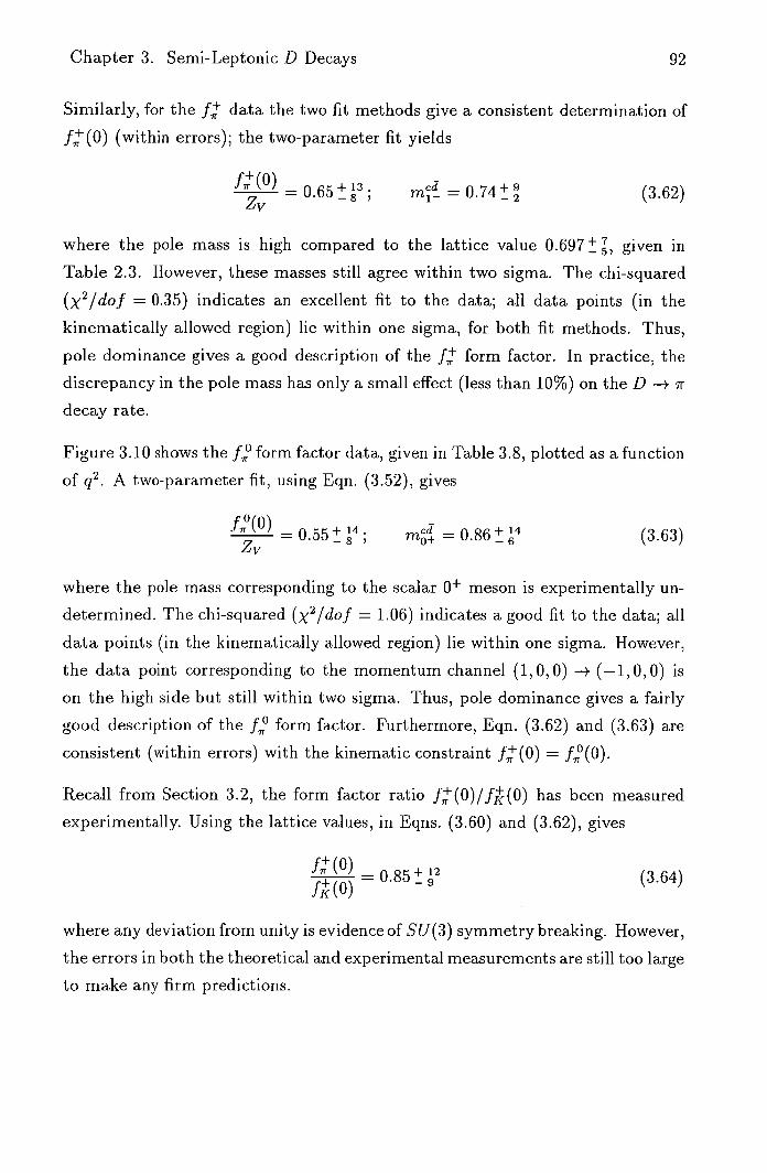
Chapter 3. Semi-Leptonic D Decays 92
Similarly, for the f data the two fit methods give a consistent determination of
f(0) (within errors); the two-parameter fityields
f_( 0 ) -
065+13 cd - —8 m 1 _ = 0.74t (3.62) zV
where the pole mass is high compared to the lattice value 0.697 t , given in
Table 2.3. However, these masses still agree within two sigma. The chi-squared
(x2/dof = 0.35) indicates an excellent fit to the data; all data points (in the
kinematically allowed region) lie within one sigma, for both fit methods. Thus,
pole dominance gives a good description of the f form factor. In practice, the
discrepancy in the pole mass has only a small effect (less than 10%) on the D - ir decay rate.
Figure 3.10 shows the f,° form factor data, given in Table 3.8, plotted as a function
of q2 . A two-parameter fit, using Eqn. (3.52), gives
f(0) - 0.55+ 14. m = 0.86 t (3.63) - —8'
where the pole mass corresponding to the scalar 0+ meson is experimentally un-
determined. The chi-squared (x 2 /dof = 1.06) indicates a good fit to the data; all
data points (in the kinematically allowed region) lie within one sigma. However,
the data point corresponding to the momentum channel (1, 0, 0) -+ (-1, 0,0) is
on the high side but still within two sigma. Thus, pole dominance gives a fairly
good description of the f1° form factor. Furthermore, Eqn. (3.62) and (3.63) are
consistent (within errors) with the kinematic constraint f(0) = f(0).
Recall from Section 3.2, the form factor ratio f(0)/f(0) has been measured
experimentally. Using the lattice values, in Eqns. (3.60) and (3.62), gives
f: ( 0) - f(0)
- 0.85 (3.64)
where any deviation from unity is evidence of SU(3) symmetry breaking. However,
the errors in both the theoretical and experimental measurements are still too large
to make any firm predictions.

Chapter 3. Semi-Leptonic D Decays
93
Pseudoscalar-to-Vector Vector Form Factors
Figures 3.11 and 3.12 show the VK* and V form factor data, given in Tables 3.9
and 3.10 respectively, plotted as a function of q2 . The VK* and V data is fitted
to the pole dominance model, given by Eqn. (3.52), as follows: the left-hand
plots correspond to a two-parameter fit; the right-hand plots correspond to a
one-parameter fit with the pole mass constrained to the mass of the associated
resonance, mD and MD. respectively.
For the VK* data the two fit methods give a consistent determination of VK.(0);
the two-parameter fit yields
VK*(0) = 1 . 15+ 13 . m= zV
-6 0.8 (3.65)
where the pole mass agrees (within errors) with both the lattice value 0.736 t ,
given in Table 2.3, and with the experimental value 2.00 0.12 i 0.18 GeV, quoted
in Section 3.2. The chi-squared (x 2 /dof >> 1) indicates a bad fit to the data.
Similarly, for the V data the two fit methods give a consistent determination of
V(0); the two-parameter fit yields
- m=0.9 zv -
(3.66)
where the pole mass is high compared to the lattice value 0.697 j , given in
Table 2.3. However, these masses still agree within two sigma. The chi-squared
(x 2 /dof >> 1) indicates a bad fit to the data. Thus, pole dominance appears to
give a poor description of the VK* and V form factors.
In Figure 3.11 the data point closest to q 2 = 0 is high (more than two sigma), in
both plots. This point corresponds to the momentum channel (0,0,0) -+ (1, 0,0)
with PD = (0, 0, 0); the other three data points correspond to momentum channels
with PD = (1,0,0). The difference in these two data sets is probably statistical but
it may also be due to systematic effects, discussed in Section 3.6. A two-parameter
fit to the data points with PD = (1, 0, 0) only gives an acceptable chi-squared but
the pole mass is poorly determined (huge errors).

Chapter 3. Semi-Leptonic D Decays
94
2 - Pole Fit VK. : 2 Param - 2 - Pole Fit Vr : 1 Param
V.(0) = 1.15
V.(0) = 1.15 t 14
= m- =0.736 3
X 2/dof = 8.48 / 2
X 2/dof = 8.52 / 3
0
I I I I I I I I I II III 01111 III 11111111
-0.2 -0.1 0.0 0.1 -0.2 -0.1 0.0
0.1 a 2 q 2 a 2 q 2
Figure 3.11: Pole dominance plots for the VK* form factor.
2 - Pole Fit VP : 2 Param 1 - Pole Fit V, : 1 Param
- v(0) = 1.09 12 -. - v(o) = 1.07
1
- rnfl =O.9
- m 1-= 0.697
- X2/dof = 6.87 / 2 - X2/dof = 7.84 / 3
0
I I I I I I III 11111 I Oil I I 11111111 II
-0.2 -0.1 0.0 0.1 0.2 -0.2 -0.1 0.0
0.1 0.2
a 2 q 2 a 2 q 2
Figure 3.12: Pole dominance plots for the V form factor.

Chapter 3. Semi-Leptonic D Decays 95
As described above, the form factors at q2 = 0 have been extracted by fitting
the chiral-extrapolated form factor data to the pole dominance model. However,
the choice of momentum channels includes some data points close to q2 = 0. An
alternative way to obtain F(0) is to assume pole dominance and to extrapolate the
point closest to q2 = 0; constraining the pole mass to the mass of the corresponding
resonance. This method has the advantage that the extrapolation in q2 is small;
the disadvantage is that a single data point only is used.
For the f and f data, the form factors at q2 = 0 obtained by extrapolating the
corresponding data point closest to q2 = 0 agree (within errors) with the values
quoted in Eqns. (3.60) and (3.62). However, for the VK and V data this is not
the case: the two-parameter fit 'favours' the data points with PD = (1, 0, 0) but
the data point closest to q2 = 0 corresponds to PD = (0,0,0). The 'difference' in
these two data sets leads to different estimates for the form factors at zero recoil.
Thus, the final 'results' for the VK* and V, form factors are as follows:
VKS(0) - = 1 . 15 8 ; m Cs1 _ = 0.8 (3.67) zv
VP (0) - = 1 . 09+ 25 .Cd
ZV - 7 m_ = 0.9 (3.68)
where the upper errors in Eqns. (3.65) and (3.66) have been increased to include
the form factor results obtained by extrapolating the corresponding data point
closest to q2 = 0.
Pseudoscalar-to-Vector Axial Form Factors
Figures 3.13 and 3.15 show the A}.- and form factor data, given in Table 3. 11,
plotted as a function of q2 . Theand data is fitted to the pole dominance
model, given by Eqn. (3.52), as follows: the left-hand plots correspond to a two-
parameter fit; the right-hand plots correspond to a one-parameter fit with the pole
mass constrained to the value 0.9. This value corresponds to the mass of the DS,
meson ( 2.5 GeV), used to extract the form factors in Ref. [63]; the quantum
numbers of this resonance require confirmation [52].

Chapter 3. Semi-Leptonic D Decays
Pole Fit A11 . : 2 Param
= 0.66 1.0
- mtjt = 1.1
0.5
X2/dof = 5.22 / 4
Pole Fit A. : 1 Param
= 0.64 1.0
- m 1 + = 0.9
0.5 _4
X2/dof = 5.96 / 5
[.1.1 111111111 I I I I I I I I I I I 0.0111 I II I I II 1 I 1 I III
-0.2 -0.1 0.0 0.1 0.2 -0.2 -0.1 0.0
a2q2 a 2q2
Figure 3.13: Pole dominance plots for the A} form factor.
- 'Pole Fit A :1 2 Param
A,(0) = 0.58
-
X2/dof = 5.39 / 4
-0.2 0.0 0.2
a 22
Figure 3.14: Pole dominance plot for the A form factor.
1.0
0.5
0.0
0.1 0.2

Chapter 3. Semi-Leptonic D Decays 97
2
2
w 14
- Pole Fit A. : 2 Param
0
Pole Fit A. : 1 Param -
A2!fl\ - - K• J - '-'-9
- m 1 + = O.9 -
:- X2/dof = 2.87 / 3
-0.2 -0.1 0.0 0.1 -0.2 -0.1 0.0 0.1
a 2 q 2
a 2 q 2
Figure 3.15: Pole dominance plots for the A < form factor.
2
0 X2/dof = 2.03 / 2
-0.2 -0.1 0.0 0.1
a 2 q 2
Figure 3.16: Pole dominance plot for the A form factor.

Chapter 3. Semi-Leptonic D Decays 98
For the and A ' . data the two fit methods give a consistent determination of
A ' . (0) and A ' (0); the two-parameter fit yields
A '. (0) _066+6. ZA -
m~ = i.ijt (3.69)
A(0) —060 m = (3.70)
ZA -
where the pole masses agree (within errors) with the experimental value 0.9
the quoted error in the experimental measurement is due to the uncertainty in the
lattice spacing. However, the A< pole mass is poorly determined (large errors).
The chi-squared (x2/dof 1) indicate a good fit to the data for both form factors.
Thus, pole dominance gives a good description of the form factor but the q 2
dependence of the A 2 . form factor (within the kinematic region) is not well-
determined.
Figures 3.14 and 3.16 show the A and A form factor data, given in Table 3.12,
plotted as a function of q 2 . Two-parameter fits, using Eqn. (3.52), give
11 A(0) =0.58;
A(0) = 0 . 43+ 8
ZA —13
m cd = 1.0 (3.71)
cd = 0.6 (3.72)
where both pole masses agree (within two sigma) with the mass of the D 1 meson
( 2.4 GeV); the quantum numbers of this resonance require confirmation [52].
The chi-squared (x2/dof 1) indicate a good fit to the data, for both form factors.
Thus, pole dominance gives a good description of the A and A form factors.
Figures 3.17 and 3.18 show the A°<. and A ° form factor data, given in Table 3.11
and Table 3.12 respectively, plotted as a function of q 2 . The A°K. and A ° data
is fitted to the pole dominance model, given by Eqn. (3.52), as follows: the left-
hand plots correspond to a two-parameter fit; the right-hand plots correspond to
a one-parameter fit with the pole mass constrained to the mass of the associated
resonance, MD, and MD respectively.

Chapter 3. Semi-Leptonic D Decays
99
1.5
1.0
o
0.5
Pole Fit 4. : 2 Param
,
0 - +7 / AK.(0)-072..4
1.5
1.0
0 Id
0.5
' Pole Fit 4. : 1 Pararn '
- A° 0 _070+ 6
Imo0706a4
X2/dof = 1.20 / 3
0.0 -0.2 -0.1 0.0 0.1
a 2 q 2
X 2/dof = 2.72 / 4
0.0 -0.2 -0.1 0.0 0.1
a 2 q 2
Figure 3.17: Pole dominance plots for the A°K* form factor.
o
1.5
1.0
0.5
0.0
- Pole Fit : 2 Param
- A(0) = 0.66 F1'1"
Mfit =
- X2/dof = 1.37 / 3
1.5
1.0
0.5
0.0
- Pole Fit : 1 Param
A(0) = 0.66 ..
- rn0-=0666 , ,/
- X2/dof = 1.73 / 4
-0.2 -0.1 0.0
0.1 0.2 -0.2 -0.1 0.0 0.1 0.2 a 2
q 2
a 22
Figure 3.18: Pole dominance plots for the A° form factor.

Chapter 3. Semi-Leptonic D Decays 100
For the A ° K , data the two fit methods give a consistent determination of A °K.(0);
the two-parameter fit yields
A0 . (0) - 0.72 m = 0_ 0.58 i (3.73)
ZA -
where the pole mass is low compared to the lattice value 0.706 t, given in
Table 2.3. However, these masses still agree within two sigma. The fit chi-squared
(x 2 /dof = 0.40) indicates an excellent fit to the data; all data points lie within one
sigma, for both fit methods. Thus, pole dominance gives a good determination
of A°K* (0) but the q2 dependence of the A°K* form factor (within the kinematic
region) is not well-determined.
Similarly, for the A ° data the two fit methods give a consistent determination of
A ° (0); the two-parameter fit yields
A0(0) — 0. m = 0.61 (3.74)
ZA -
where the pole mass agrees (within errors) with the lattice value 0.666 t, given in
Table 2.3. The fit chi-squared (x2/dof = 0.46) indicates an excellent fit to the
data; all data points lie within one sigma, for both fit methods. Thus, pole
dominance gives a good description of the A ° form factor.
Recall from Section 3.1, the D -+ K*, p decay rates, given by Eqn. (3.19), are
proportional to an integral over q2 which is a function of V, A 1 and A 2 . For the
vector and axial form factor data, given in Tables 3.9-3.12, pole dominance gives
a good description of theand A form factors. However, the q2 dependence
of the VK*, V, A and A form factors is not well-determined. Fortunately, the
decay rate is dominated by the A 1 form factor; the V and A 2 contributions are
small and only important in the region q 2 = 0 where they are reasonably well-
determined. For example, the discrepancy in the pole-mass (a factor of two)
has only a small effect (less than 5%) on the D -* K* decay rate. Thus, the
form factor results quoted in this Section can be used to compute (with some
confidence) the total decay rates.

Chapter 3. Semi-Leptonic D Decays
101
3.6 Renormalisation Constants
In this section, the problem of determining the D -* K, .K* and D -+ ir, p form
factors due to discretisation errors is discussed. In this study, discretisation errors
are substantially reduced by the use of the 0(a)-improved SW action. However,
for currently accessible lattice spacings these errors lead to an uncertainty of order
10% in the form factors.
Renormalisation Constant Definition
The lattice currents Vt and A used in this study are related to the physical ones
(V's and A) by renormalisation constants Zv and ZA as follows:
Z' V = V (3.75)
ZA A = A' (3.76)
where V yQ and A = are the vector and axial heavy-light currents
respectively.
Light-Light Current
A UKQCD study [64] of the light-light current qyq for the SW action at / = 6.2
(using chiral Ward identities) obtained
Zv = 0.81728 (3.77)
where the first error is statistical, the second is due to the mass dependence of
Zv corresponding to Ki = 0.14144, 0.14226 and 0.14262; Zv increases linearly
with increasing light quark mass. This result is in good agreement with the
one-loop perturbative value 0.83 [65]—[66] computed using a 'boosted' coupling
constant [67]. Similarly, a study of the light-light current q -y7 5 q obtained
ZA = 1.05i1 (3.78)
which is higher than the perturbative value 0.97. However, no dependence on the
light quark mass was observed. Thus, when both quarks are light the discretisation
errors are small.

Chapter 3. Semi-Leptonic D Decays
102
Heavy-Light Current
A UKQCD study [19] of the heavy-heavy vector current Q'yQ was performed by
defining an effective Zv as follows:
jj - ________________ 'UV
- G (3.79)
p (t,t,0;p)E
with
G 2' ( t, 0; j) = ( o 11
{ P(y) Pt(o)} 0) (3.80)
t, 0; j3) = et (°l t {P( y ) V'(x) Pt(o)} 0) (3.81) , 7
where Pt and P are interpolating operators to create and annihilate a heavy-light
pseudoscalar meson respectively.
For degenerate heavy quarks with kh = 0.129, and using correlation functions with
j= 0 and ,a = 4, gives
Z eff = 0.9177 (3.82)
which differs by about 10% from the value 0.83 determined using light quarks.
This difference is a measure of the size of the discretisation errors for the SW action
which are of O(a3 ma) and O(m 2 a2 ). For the Wilson action the discretisation
errors are much larger, O(ma).
Furthermore, it is important to realise that discretisation errors of O(ama) and
O(m 2 a2 ) are, in general, different for matrix elements with different Lorentz in-
dices and between different states. Thus, these errors cannot be absorbed into
universal (effective) Zv and ZA. Fortunately, hypercubic group invariance ensures
there are no discretisation errors of O(ama) which affect spatial components dif-
ferently from temporal components, for each q2 value. However, even if O(m 2 a2 )
corrections are neglected (in which case discretisation errors are independent of
the Lorentz current) these errors could be different for different form factors, and
they could have a different q2 dependence than the form factors themselves.

Chapter 3. Semi-Leptonic D Decays 103
Effective Renormalisation Constants
In this study, the discretisation errors are modelled by using effective (mass-
dependent) renormalisation constants, Z/ 1 and Z/1 , in an attempt to absorb
at least part of the error. For the vector current an approximate average of the
perturbative value 0.83 (obtained using light quarks) and the non-perturbative
value 0.92 (obtained using heavy quarks) gives
Z/ 1 = 0.88j. (3.83)
For the light-light axial current the perturbative and non-perturbative determina-
tions of ZA do not agree. Thus, the 'best' estimate for the axial renormalisation
constant is
Z = 1.05th (3.84)
which corresponds to the non-perturbative result but with the lower error
increased to include the perturbative value.
3.7 Comparison with Experiment
In Section 3.5, the D -+ K, K* and D -4 7r, p form factor data was fitted to
the pole dominance form, given by Eqn. (3.52), to obtain the form factors at
q2 = 0 and the corresponding pole masses. In this section, the form factors are
compared with experiment and other theoretical calculations. In order to make
this comparison, values for the renormalisation constants Zv and ZA must be
specified. The D -+ K, K* and D -+ ir, p decay rates, given by Eqns. (3.18)
and (3.19), are also computed; the integrals (over q2 ) were performed analytically
by assuming pole-dominance for the form factors.
Physical Form Factors
The D - K, K" and D -+ 7r, p form factors at q2 = 0, obtained from pole dom-
inance fits in Section 3.5, are given in Tables 3.13 and 3.14 respectively, using
effective renormalisation constants Z/ = 0.88 and Z 11 = 1.05 , as detailed
in Section 3.6. The experimental world average, and other theoretical results are
quoted for comparison.

Chapter 3. Semi-Leptonic D Decays 104
Source Reference 11 f(0) VK.(0)
World Ave. [68] 0.70+0.03 N/A Exp't
World Ave. [69] 0.77+0.04 1.16+0.16
Lattice This Work 0.67 j 0.05 + 0.03 0.03 - 0.04
1 . 01 + 0.25 + 0.05 - 0.05 - 0.06
Clover APE [70] 0.780.08 1.080.22
LANL [71] 0.71+0.04 1.28+0.07
Wuppertal [72] 0.71t0 1.1 2+0.10 -0.07 1-34+0.24
Lattice LMMS [73] 0.63+0.08 0.86+0-10
Wilson BKS [74] 0.90 0.08 ' 0.21 1.43+0.45+ 0.49
ELC [75] 0.60 + 0.15 + 0.07 0.86i 0.24
ISOW [76] 0.76-0.82 1.1
Quark WSB [77] 0.76 1.27
Models KS [78] 0.76 0.8
GS [79] 0.69 1.5
BBD [80] 0.60+ 0.15 -0.10 1.10+0.25 -
Sum Rules AEK [81] 0.60+0.15 N/A
DP [81] 0.75i 0.05 N/A
Table 3.13: D -+ K, K' form factors: Theory vs. Experiment.

Chapter 3. Semi-Leptonic D Decays
105
Source Reference A ' . (0) A 2K (0)
Exp't World Ave. [69] 0.61+0.05 0.45 i 0.09
Lattice This Work 0.69+0' 06+0.01 0.03-0.05 0.63 t 0.12 + 0.01
- 0.05
Clover APE [70] 0.67+0-11 0.49+0.34
LANL [71] 0.72i 0.03 0.49+0.09
Wuppertal [72] 0.61 i 0.06 i 0.83 ii 0 20 + 0.12 -0.08
Lattice LMMS [73] 0.53+0.03 0.19i 0.21
Wilson BKS [74] 0.83 0.14 0.28 0.59 0.14 0.23
ELC [75] 0.64+0.16 0.40 0.28 ii 0.04
ISGW [76] 0.8 0.8
Quark WSB [77] 0.88 1.15
Models KS [78] 0.82 0.8
GS [79] 0.73 0.55
Sum Rules BBD [80] 0.50+0.15 0.60+0.15
Table 3.13: (Cont.)

Chapter 3. Semi-Leptonic D Decays wo
Source Reference VK.(0)/A.(0) A(0)/A'j < (0)
Exp't World Ave. [69] 1.90+0.25 0.74+0.15
Lattice This Work 1.47 0.05 0.90.10.1
Clover APE [70] 1.60.3 0.70.4
LANL [71] 1.78+0.07 0.68+0.11
Lattice LMMS [73] 1.60.2 0.40.4
Wilson BKS [74] 1.99+0.22+ 0-31 0.70 0.16 ii 0.20
ELC [75] 1.3+0.2 0-6+0-3
ISGW [76] 1.40.4 1.0t0.3
Quark WSB [77] 1.4 1.3
Models KS [78] 1.0 1.0
CS [79] 2.0 0.8
Sum Rules BBD [80] 2.20.2 1.20.2
Table 3.13: (Cont.)

Chapter 3. Semi-Leptonic D Decays
107
Source Reference 11 f: (0) 1 V, ( 0 )
Clover This Work 0.57 + 0 - 11 0.03 0.96 I 0.22+ 0.04 -0.06 - 0.06
Wuppertal [72] 0.68 t 0.13 1.31 0.25 + 0.18 -0.13
Lattice LMMS [73] 0-58+0.09 0.77+0.09
Wilson BKS [74] 0.84i 0.12 j 0.35 1.07 0.49 0.35
ISOW [76] 0.51 N/A Quark
WSB [77] 0.69 1.23 Models
KS [78] 0.69 1.23
Sum Rules AEK, DP [81] 0.6-0.75 N/A
Source Reference A(0) [
A(0)
Clover This Work 0.61+ 0.06+0.01 - 0.03-0.05 0.14 - 0.03
[ 0.45 + 0.08 + 0.01
Wuppertal [72] 0.59 + 0.07 + °° - -0.06 0.83 i 0.20 t 0.12 0.08
Lattice LMMS [73] 0.47+0.07 -0.07+0.42
Wilson BKS [74] 0.65+0.15+ 0.24 - - 0.23 0.59 + 0.28
- 0.25
Quark WSB [77] 0.78 0.92
Models KS [78] 0.78 0.92
Table 3.14: D - ir, p form factors.

Chapter 3. Semi-Leptonic D Decays 108
The errors quoted for 'This Work', in Tables 3.13 and 3.14, correspond as follows:
the first set are statistical, the second are due to the uncertainty in the effective
renormalisation constants, computed using the extreme values of ZR and Zeff
However, the systematic error for the ratio A(0)/A <.(0) corresponds to an esti-
mate of the uncertainty in ZAeff for different form factors. Recall from Section 3.6,
different form factors could have different discretisation errors. Thus, the effective
renormalisation constant Z/' may be different for A' than for A 2 ; this leads to
an additional ambiguity of 10% for this ratio. The errors quoted for 'Other Work'
correspond as follows: the first error is statistical, the second is an estimate of the
systematic error.
The D -+ K, K" form factors obtained in this study are in good agreement with
experimental measurements (all results agree within 1.5 sigma), and with the
most recent lattice simulations using 0(a)-improved SW [70] and Wilson [71, 72]
actions. The values reported in Refs. [73, 75] and [74] (obtained in the pioneering
lattice studies using Wilson fermions) are also in agreement but the former are,
in general, lower and the latter higher than the predictions made in this study.
In principle, discretisation errors are larger for Wilson than for 0(a)-improved
SW actions. However, part of the discrepancy in the lattice results is due to the
different values used in the literature for the effective renormalisation constants,
Z/ 1 and Z 11 . The lattice results are also in agreement with quark-model and
sum-rule predictions.
The D -+ it, p form factors obtained in this study are in excellent agreement with
other lattice results, and with quark-model and sum-rule predictions. However,
there are no experimental measurements available for these form factors. Thus,
the lattice is the only source of quantitative results for the D —* 7r, p form factors.
Decay Rates
The D -* K, K"' and D -+ it, p decay rates, computed using lattice masses with
IVc8 I = 0.975 and IVcd I = 0.222 [52], are given in Table 3.15. The experimental.
world average, and other theoretical results are quoted for comparison. Ref [69]
gives F(D —+ r) = 1.2 i 0.3 10 10 s_I. Assuming isospin symmetry, one obtains the
decay rate F(D -+ iri!) = 0.60t 0.15 1010 _i, quoted in Table 3.15, with charged
pions in the final state.
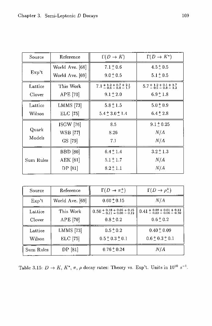
Chapter 3. Semi-Leptonic D Decays
109
Source Reference F(D - K) F(D K)
World Ave. [68] 7.1 + 0.6 4.5+0.5 Exp't
World Ave. [69] 9.00.5 5.1+0.5
Lattice This Work 7.1 + 1.2 + 0.7 + 2.1 - 0.6 -0.8- 1.7 -' ' +
1.2 + 0.1 + 1.7 - 0.5-0.8-1.3
Clover APE [70] 9.12.0 6.91.8
Lattice LMMS [73] 5.8+1.5 5.00.9
Wilson ELC [75] 5.4k 3.0k 1.4 6.4+2.8
ISGW [76] 8.5 9.1+0.25 Quark
WSB [77] 8.26 N/A Models
GS [79] 7.1 N/A
BBD [80] 6.4+1.4 3.2+1.3
Sum Rules AEK [81] 5.1+1.7 N/A
DP [81] 8.21.1 N/A
Source Reference F(D -* irk) F(D -4 p)
Exp't World Ave. [69] 0.60+0.15 N/A
Lattice
Clover
This Work
APE [70]
0.50 + 0.18 + 0.05 + 0.15 - 0.11 - 0.06 - 0.12
0.8+0.2
0 41 + 0.09 + 0.01 + 0.12 - 0.03 - 0.06 - 0.10
0.6+0.2
Lattice
Wilson
LMMS [73]
ELC [75]
0.5+0.2
0.5 + 0.3 + 0.1
0.40+0.09
0.6 t 0.3 + 0.1
Sum Rules DP [81] 0.76+0.24 ]
N/A
Table 3.15: D -+ K, K', ir, p decay rates: Theory vs. Exp't. Units in 1010 s_i

Chapter 3. Semi-Leptonic D Decays 110
Source Reference IT(D-+K) I FL(D*K*) F(D-*K) rT(D.*K*)
Exp't World Ave. [68] 0.55+0.07 1.2t0.1
Lattice This Work 0.800.05 1.120.01
Clover APE [70] 0.80.3 1.20.3
Lattice LMMS [73] 0.86+0.22 1.51+0.27
Wilson ELC [75] 1.10.60.3 1.40.3
ISGW [76] 1.1 1.1+0.2
Quark WSB [77] 1.15 0.9
Models KS [78] 0.95 1.1
GS [79] 1.4 1.2
Sum Rules BBD [80] 0.50+0.15 0.86+0.06
Table 3.15: (Cont.)

Chapter 3. Semi-Leptonic D Decays 111
For the pseudoscalar-to-pseudoscalar decay, Z!f is an overall factor in the
decay rate, given by Eqns. (3.18). Therefore, this result could be quoted in
terms of F(D -+ K)/(ZP)2 . However, for the pseudoscalar-to-vector decay such a
factorisation is not possible; the Hi form factors mix the vector and axial con-
tributions, given by Eqn. (3.19). Therefore, both decay rates are computed using
effective renormaljsation constants= 0.88 and Z 11 = 1.05 + , as detailed
in Section 3.6.
The errors quoted for 'This Work', in Table 3.15, correspond as follows: the first
set are statistical; the second are due to the uncertainty in the effective renormal-
isation constants Zv and ZA; the third are due to the uncertainty in the inverse
lattice spacing, computed using the extreme values of a 1 = 2.85 0.15 GeV. The
errors quoted for 'Other Work' correspond as follows: the first error is statistical,
and the second is an estimate of the systematic error.
The D -4 K, K and D -* ir, p decay rates obtained in this study are in
excellent agreement with experimental measurements, other lattice results, and
quark-model and sum-rule predictions. For the decay D -+ p, the lattice provides
the only quantitative result for the decay rate. In this study, the uncertainty in
the inverse lattice spacing is the largest source of error in determining the decay
rates.
Summary and Conclusions
This thesis describes a lattice calculation of the matrix elements of the vector
and axial-vector currents which are relevant for the semi-leptonic decays D -+ K
and D - K* . The simulation was performed in the quenched approximation to
lattice QCD on a 24 x 48 space-time lattice at 0 = 6.2, using the 0(a)-improved
Sheikholeslami-Wohlert (SW) action.
In the limit of zero lepton masses the D -+ K and D -+ K* decays are described
by four form factors: f, VK*, A<. and which are dimensionless functions
of q2 , where q 11 is the four-momentum transfer. The D -+ K and D -+ K* form
factors were determined for different q2 values; their q2 dependence is found to be
reasonably well described by a simple pole-dominance model. In particular, f andare well determined over the entire kinematically allowed range; these
form factors dominate the D -+ K and D -+ K* decay rates respectively. The
D -+ it and D -p p form factors were also determined.
The form factor results at q2 = 0, obtained from pole-dominance fits, are in good
agreement with experiment and other theoretical calculations. The D -+ K, K*
and D -+ it, p decay rates were also computed; the integrals over q2 are performed
analytically by assuming pole dominance. Again, these results are in good agree-
ment with experiment. This agreement gives further confidence that lattice QCD
is becoming a reliable quantitative tool for non-perturbative QCD phenomenology.
This study is one of the first calculations of weak matrix elements using the 0(a)-
improved SW action. Furthermore, a large lattice volume is used to minimise
finite-size effects. Nevertheless, discretisation errors are still of order 10% for
the form factors. Thus, it is important to repeat this calculation on lattices of
different sizes and lattice spacings in order to study these systematic errors (except
quenching) in detail. In the next few years, lattice calculations in full QCD will
be performed giving control over all systematic errors.
112

References
I. Aitchison and A. Hey, Gauge Theories in Particke Physics,
Adam Huger (1989).
T. Cheng and L. Li, Gauge Theory of Elementary Particle Physics,
Oxford University Press (1984).
L. Ryder Quantum Field Theory, Cambridge University Press (1986).
N. Cabibbo, Phys. Rev. Lett. 10 (1963) 531.
M. Kobayashi and K. Maskawa, Prog. Theor. Phys. 49 (1973) 652.
P. Higgs, Phys. Rev. Lett. 12 (1964) 132.
R.P Feynman and M. Cell-Mann, Phys. Rev. 109 (1958) 193.
E. Sudarshan and R. Marshak, Phys. Rev. 109 (1958) 1860.
J.J. Sakurai, Nuovo Cimento 7 (1958) 649.
G. Martinelli, and C. Bernard and A. Soni in Lattice 88,
Nuel. Phys. B (Proc. Suppl.) 9 (1989) 134 and 155.
S. Sharpe in Lattice 89, Nucl. Phys. B (Proc. Suppi.) 17 (1990) 146.
G. Kilcup in Lattice 90, NucI. Phys. B (Proc. Suppi.) 20 (1991) 417.
C. Martinelli in Lattice 91, NucI. Phys. B (Proc. Suppl.) 26 (1992) 31.
C.T. Sachrajda in Lattice 92, Nuci. Phys. B (Proc. Suppi.) 30 (1993) 20.
C. Bernard in Lattice 93, Nucl. Phys. B (Proc. Suppi.) 34 (1994) 47.
S.P. Booth et al. (UKQCD), Phys. Rev. Lett. 72 (1994) 462.
K.C. Bowler et al. (UKQCD), Phys. Rev. Lett. 72 (1994) 1398.
113

REFERENCES
114
K.C. Bowler et at. (UKQCD), Phys. Rev. D51 (1995) 4955.
K.C. Bowler et al. (UKQCD), Phys. Rev. D52 (1995) 5067.
D.R.Burford et al. (UKQCD), Nucl. Phys. B447 (1995) 425.
J.M. Flynn et at. (UKQCD), NucI. Phys. B461 (1996) 327.
M. Creutz, Quarks, Gluons and Lattices,
Cambridge University Press (1983).
I. Montvay and G. Mflnster, Quantum Fields on a Lattice,
Cambridge University Press (1994).
C. Rebbi, Lattice Gauge Theories and Monte Carlo Simulations,
World Scientific (1983).
H.J. Rothe, Lattice Gauge Theories, World Scientific (1992).
D. Gross and F. Wilczek, Phys. Rev. Lett. 30 (1973) 1343.
S. Weinberg, Phys. Rev. Lett. 31 (1973) 494.
H. Fritzsch, M. Cell-Mann and H. Leutwyler, Phys. Lett. 47B (1973) 365.
A. Zee, Phys. Rev. D7 (1973) 3630.
S. Coleman and D.J. Gross, Phys. Rev. Lett. 31 (1973) 851.
B. Schutz, Geometrical Methods of Mathematical Physics,
Cambridge University Press (1980).
R.P. Feynman and A.R. Hibbs, Quantum Mechanics and Path Integrals,
McGrawHill (1965).
N. Metropolis, A.W. Rosenbiuth, M.N. Rosenbluth, A.H. Teller and
E. Teller, J. Chem. Phys 21 (1953) 1087.
K.G. Wilson, in New Phenomena in Subnuclear Physics, Erice Lectures,
Ed. A.Zichichi, Plenum Press (1975).
K.G. Wilson, Phys. Rev. D14 (1974) 2455.

REFERENCES
115
M. Luscher and P. Weisz, Commun. Math. Phys. 97 (1985) 59.
H.W. Hamber and C.M. Wu, Phys. Lett. B136 (1984) 255.
B. Sheikholeslami and R. Wohiert, Nucl. Phys. B259 (1985) 572.
G. Heatlie et at., Nuci. Phys. B352 (1991) 266.
J. Mandula et al., Nuci. Phys. B228 (1983) 109.
W.H. Press et at., Numerical Recipes in C, Second Edition,
Cambridge University Press (1992).
S. Cusken et al. in Lattice 89,
Nuci. Phys. B (Proc. Suppi.) 17 (1990) 361; Phys. Lett. B227 (1989) 266.
F. Mandl and C. Shaw, Quantum Field Theory, Wiley (1984).
C. Bernard, A. E1-Khadra and A. Soni,
Nucl. Phys. B (Proc. Suppi.) 9 (1989) 186; 17 (1990) 499.
C.R. Aliton et al. (UKQCD), Phys. Rev. D49 (1994) 474.
C.R. Aliton et at. (UKQCD), Nuci. Phys. B407 (1993) 331.
R.M. Baxter et al. (UKQCD), Phys. Rev. D49 (1994) 1594.
A.D. Simpson, Ph.D. Thesis, The University of Edinburgh (1991).
B. Efron, The Jackknife, the Bootstrap and other Resampling Plans,
Society for Industrial and Applied Mathematics (1982).
G. Wetherill, Elementary Statistical Methods, Chapman and Hall (1982).
W.H. Press et al., Numerical Recipes in C, Cambridge Press (1988).
Particle Properties, Phys. Rev. D45 (1992).
P.L. Frabetti et at. (E-687), Phys. Lett. B315 (1993) 203.
G. Crawford et at. (CLEO), Phys. Rev. D44 (1991) 3394.
Z. Bai et al. (MARK III), Phys. Rev. Lett. 66 (1991) 1011.

REFERENCES
116
J.C. Anjos et at. (E-691), Phys. Rev. Lett. 62 (1989) 1587.
A. Bean et al. (CLEO), Phys. Lett. B317 (1993) 647.
J. Adler et at. (MARK III), Phys. Rev. Lett. 62 (1989) 1821.
M.S. Alam et at. (CLEO), Phys. Rev. Lett. 71 (1993) 1311.
P.L. Frabetti et at. (E-687), Phys. Lett. B307 (1993) 262.
K. Kodama et at. (E-653), Phys. Lett. B274 (1992) 246; B286 (1992) 187.
H. Albrecht et at. (ARGUS), Phys. Lett. B255 (1991) 634.
J.C. Anjos et at. (E-691), Phys. Rev. Lett. 65 (1990) 2630; 62 (1989) 722.
D.S. Henty et at. (UKQCD), Phys. Rev. D51 (1995) 5323.
E. Gabrielli et at., Nuct. Phys. B362 (1991) 475.
A. Borrelli et at., Nuci. Phys. B409 (1993) 382.
G.P. Lepage and P.B. MacKenzie,
Nucl. Phys. B (Proc. Suppi.) 20 (1991) 173.
G. Bellini, talk given at Les Rencontres de Physique de la Vallee d'Aoste,
La Thuile, Aosta Valley (1994).
M.S. Witherell, talk given at the mt. Symposium on Lepton and Photon
Interactions at High Energies, Cornell University, Ithaca, NY (1993).
C.R. Ailton et at. (APE), Phys. Lett. B345 (1995) 513.
T. Bhattacharya and R. Gupta,
Nuct. Phys. B (Proc. Suppi.) 42 (1995) 935.
S. Güsken, et at., preprint HLRZ-95-38.
M. Crisafulli, G. Martinelli, V.J. Hill and C.T. Sachrajda,
Phys. Lett. B223 (1989) 90; V. Lubicz, G. Martinelli and C.T. Sachrajda,
Nuct. Phys. B356 (1991) 301; V. Lubicz, G. Martinelli, M.S. McCarthy and
C.T. Sachrajda, Phys. Lett. B274 (1992) 415.

REFERENCES 117
C. Bernard, A. E1-Khadra and A. Soni, Phys. Rev. D43 (1991) 2140;
D45 (1992) 869.
A. Abada, et al., Nuci. Phys. B416 (1994) 675.
D. Scora and N. Isgur, Phys. Rev. D40 (1989) 1491;
N. Isgur, D. Scora, B. Grinstein and M. Wise, Phys. Rev. D39 (1989) 799.
M. Bauer, B. Stech and M. Wirbel, Z. Phys. C29 (1985) 637;
C34 (1987) 103; M. Bauer and M. Wirbel, ibid. 42 (1989) 671.
J.G. Körner and G.A. Schuler, Z. Phys. C38 (1988) 511; C46 (1990) 93;
Phys. Lett. B231 (1989) 306.
F.J. Gilman and R.L. Singleton, Phys. Rev. D41 (1990) 142.
P. Ball, V.M. Braun, H.G. Dosch and M. Neubert,
Phys. Lett. B259 (1991) 481; P. Ball, V.M. Braun and H.G. Dosch,
Phys. Rev. D44 (1991) 3567.
T.M. Aliev, V.L. Eletskii, and Y.I. Kogan,
Soy. J. Nuci. Phys. 40 (1984) 527;
C.A. Dominguez and N. Paver, Phys. Lett. B207 (1988) 499.