Embed Size (px)
Citation preview

EPA 600/R-14/383 | January 2015 | www.epa.gov/research
Systems Measures of Water Distribution System Resilience
Office of Research and DevelopmentNational Homeland Security Research Center

ii
Acknowledgements The United States Environmental Protection Agency (EPA) would like to acknowledge Regan
Murray (EPA), Katherine Klise, Cynthia Phillips, and LaTonya Walker (Sandia National
Laboratories) for their contributions to this report, and Joseph Fiksel (The Ohio State
University), Carl Laird (Purdue University), Jonathan Burkhardt (Oak Ridge Institute for Science
and Education Fellow), Keely Maxwell (American Association for the Advancement of Science
Policy Fellow), Eli Walton (Student Services Contractor), Steve Clark, Brendan Doyle, Terra
Haxton, and Robert Janke(EPA) for technical review of this report.
Questions concerning this document or its application should be addressed to:
Regan Murray USEPA/NHSRC (NG 16) 26 W Martin Luther King Drive Cincinnati OH 45268 (513) 569-7031 [email protected]
Disclaimer The U.S. Environmental Protection Agency (EPA) through its Office of Research and
Development funded and collaborated in the research described here under an Inter-Agency
Agreement with the Department of Energy’s Sandia National Laboratories. It has been
subjected to the Agency’s review and has been approved for publication. Note that approval
does not signify that the contents necessarily reflect the views of the Agency. Mention of trade
names, products, or services does not convey official EPA approval, endorsement, or
recommendation.

iii
Contents Acknowledgements ......................................................................................................................ii
Disclaimer .....................................................................................................................................ii
List of Figures................................................................................................................................ v
List of Acronyms and Abbreviations............................................................................................ vi
1 Introduction ............................................................................................................................. 1
2 Resilience of Drinking Water Systems ..................................................................................... 4
2.1 Drinking Water Hazards ................................................................................................... 4
2.2 Enhancing Preparedness for Hazards............................................................................... 5
2.3 Drinking Water Resilience Tools ...................................................................................... 6
3 Measuring Resilience ............................................................................................................... 9
3.1 Understanding Resilience ................................................................................................. 9
3.1.1 Resilience, Risk, Vulnerability, and Preparedness .................................................. 10
3.1.2 Resilience Attributes and Indicators ....................................................................... 12
3.1.3 Resilience as a Systems Concept ............................................................................ 14
3.2 Approaches to Measuring Resilience ............................................................................. 15
3.2.1 Qualitative Approaches .......................................................................................... 15
3.2.2 Systems Modeling Approach .................................................................................. 17
4 Quantitative Performance Measures .................................................................................... 20
4.1 Risk ................................................................................................................................. 20
4.2 Resilience ........................................................................................................................ 21
4.2.1 Time-based Resilience Assessment ........................................................................ 22
4.3 Reliability ........................................................................................................................ 23
4.3.1 Topological Reliability ............................................................................................. 24
4.3.2 Hydraulic Reliability ................................................................................................ 26
4.3.3 Entropy Reliability ................................................................................................... 29
4.4 Standard Performance Measures .................................................................................. 30
4.4.1 Cost ......................................................................................................................... 30
4.4.2 Water Quality .......................................................................................................... 31
4.4.3 Water Pressure ....................................................................................................... 32

iv
4.5 Other Performance Metrics ........................................................................................... 34
4.5.1 Greenhouse Gas Emissions ..................................................................................... 34
4.5.2 Water Security ........................................................................................................ 34
4.5.3 Social Welfare Functions ......................................................................................... 36
5 Discussion .............................................................................................................................. 38
6 Conclusions ............................................................................................................................ 42
References .................................................................................................................................... 44

v
List of Figures Figure 1 Continuous cycle of building resilience to hazards. .......................................................... 2
Figure 2 Potential hazards and impacts to drinking water systems. .............................................. 5
Figure 3 System performance function before, during, and after an event. ............................... 10
Figure 4 Schematic of a drinking water “system” with all its interacting component parts: the
physical components, the services it provides, the organizations that govern it, and the people
and industry that consume it. ....................................................................................................... 15
Figure 5 Schematic of a distribution network with two sources (lake and river) and three tanks.
....................................................................................................................................................... 18

vi
List of Acronyms and Abbreviations ASCE American Society of Civil Engineers
AWWA American Water Works Association
CBRN chemical, biological, radiological and nuclear
CBWR Community Based Water Resiliency
CIPAC Critical Infrastructure Partnership Advisory Council
CREAT Climate Resilience Evaluation and Awareness Tool
DMA district metered areas
EPA U.S. Environmental Protection Agency
EPANET Hydraulic and water quality modeling software for pipe networks
GHG greenhouse gas
gpm gallons per minute
HRD Hydraulic Reliability Diagram
IFRC International Federation of Red Cross
NAS National Academies of Science
NEDRA Network Design and Reliability Assessment
NIAC National Infrastructure Advisory Council
NPR node pair reliability
psi pounds per square inch
PSPF Percentage of Demand Supplied at adequate Pressure
RAMCAP Risk Analysis and Management for Critical Asset Protection
SCADA supervisory control and data acquisition
WDS water distribution systems
WPR Water Provision Resilience
WST Water Security Toolkit

1
1 Introduction Drinking water security is the ability to access an
adequate amount of good quality water to support
human health, the economy, and the environment. It
also means protecting drinking water from a wide
variety of hazards including natural disasters, climate
change, and terrorist attacks. Building resilience to
these hazards is key to improving water security.
U. S. Presidential Policy Directive (PPD) 21 – Critical
Infrastructure Security and Resilience – establishes
national policy to build resilience to hazards. PPD 21
directs federal agencies to work with critical
infrastructure owners and operators and state, local,
tribal, and territorial entities to “take proactive steps to
manage risk and strengthen the security and resilience
of the Nation’s critical infrastructure, … These efforts
shall seek to reduce vulnerabilities, minimize
consequences, identify and disrupt threats, and hasten response and recovery efforts related to
critical infrastructure.” Water and wastewater systems are identified as one of sixteen critical
U. S. infrastructure; resilience of the water sector is tightly linked to the resilience of other
critical infrastructure such as energy, food and agriculture, healthcare and public health.
Disaster resilience is defined by the National Academies of Science as the ability of a human
system (e.g., an individual, community, or the nation) to prepare and plan for, absorb, recover
from, and successfully adapt to adverse events (NAS, 2012). The Community and Regional
Resilience Institute (CARRI) defined community resilience as “the ability to anticipate risk, limit
impacts, and bounce back rapidly in the face of turbulent change” (CARRI, 2014). The National
Infrastructure Advisory Council (NIAC) defined infrastructure resilience as “the ability to reduce
the magnitude and/or duration of disruptive events. The effectiveness of a resilient
infrastructure or enterprise depends upon its ability to anticipate, absorb, adapt to, and/or
rapidly recover from a potentially disruptive event” (NIAC, 2009). Here, infrastructure refers to
the facilities and equipment comprising the physical infrastructure, the services provided to a
community by the infrastructure, the people using the services, and the organizations that
manage the infrastructure. By these definitions, resilience of human systems to natural
disasters and other hazards implies a continuous cycle of planning and preparedness activities,
“Water security is defined as
the capacity of a population to
safeguard sustainable access
to adequate quantities of
acceptable quality water for
sustaining livelihoods, human
well-being, and socio-
economic development, for
ensuring protection against
water-borne pollution and
water-related disasters, and
for preserving ecosystems in
a climate of peace and
political stability.”
–United Nations-Water Task
Force on Water Security,
2013

2
response and recovery actions following an adverse event, and adapting and changing to be
better prepared for future events based on lessons learned (see Figure 1).
Figure 1 Continuous cycle of building resilience to hazards.
These definitions of resilience also highlight the importance of defining who or what is resilient,
and to what they are resilient. In this report, the focus is on the resilience of drinking water
systems to natural disasters, terrorist attacks, and other hazards. Resilience of drinking water
systems refers to the ability of the human organizations that manage water to design, maintain,
and operate water infrastructure (e.g., water sources, treatment plants, storage tanks, and
distribution systems) in such a way that limits the effects of disasters on the water
infrastructure and the community it serves, and enables rapid return to normal delivery of safe
water to customers. Many organizations have written about the resilience of drinking water
systems to natural disasters, terrorist attacks, and other emergencies over the last several years
(ASCE, 2008; CIPAC Workgroup, 2009; ANSI, 2010; USEPA, 2011 and 2012a) providing useful
information on preparedness, response and recovery, case studies and lessons learned, and
water sector specific tools.
Preparedness & Mitigation
Event
Response & Recovery
Lessons Learned & Adaptation

3
One of the challenges to using the concept of resilience is determining how to quantify or
measure resilience. With limited resources, water utilities must make decisions about which
preparedness and adaptation activities will most improve their resilience. Measures of
resilience would help in prioritizing such decision making; however, satisfactory measures or
indicators of resilience are not currently available. As described in McAllister (2013), resilience
performance goals and quantitative metrics are needed that can be used to support risk-based
decision-making at water systems.
This report reviews quantitative performance measures for water distribution systems with a
focus on systems measures that can be used to quantify resilience to natural disasters, terrorist
attacks, and other hazards. In the next section, literature and tools to support the resilience of
drinking water systems are reviewed. Then, resilience characteristics, attributes, and systems
analysis approaches are reviewed for their relevance to quantifying the resilience of drinking
water systems to hazards. Existing water system performance measures are presented and
reviewed. Finally, the advantages of using these measures to quantify resilience to hazards is
considered and necessary improvements to systems analysis tools are outlined. This report
provides an overview of potential resilience measures, however, additional research is needed
to formulate meaningful quantitative systems measures for resilience and incorporate them
into tools for water distribution systems.

4
2 Resilience of Drinking Water Systems Drinking water systems have been significantly impacted by natural disasters and hazardous
releases. Hurricane Katrina, Superstorm Sandy, the West Virginia’s 2014 Elk River chemical
spill, and the 2014 Lake Erie algal bloom have all significantly impacted drinking water systems
and received national attention (Reed et al., 2013; Scharfenaker, 2006; Sewerage and Water
Board of New Orleans, 2013; WARN, 2013; DiGiano and Grayman, 2014; Osnos, 2014). This
section reviews the many potential hazards facing drinking water systems, guidance on
preparedness, and existing drinking water resilience tools.
2.1 Drinking Water Hazards
Across the United States, water systems face multiple challenges on a daily basis. Water
systems plan and prepare for natural disasters, hazardous material releases, cyber-attacks, and
terrorist attacks. Utilities strive to maintain and retrofit aging infrastructure in an effort to
minimize water quality problems, leaks, and pipe breaks. In addition, utilities plan for
uncertainty in water supply and demand due to climate change and shifting population centers.
Figure 2 lists a variety of potential hazards to water distribution systems and the resulting
impacts to the water system (adapted from CIPAC Workgroup, 2009). Each of the hazards in
the first box could result in multiple impacts listed in the second box. For example, a 2011
drought in Texas caused pipes to break because of shifting soils and caused some water sources
to dry up (Llanos, 2011), resulting in both pipe breaks and service disruptions. The 2011
Tropical Storm Irene caused power outages, damaged roads and bridges which caused pipe
breaks and limited transportation of water treatment chemicals, and released hazardous waste
that impacted the quality of water sources (Vermont Department of Natural Resources, 2011).
The 2007 Angora Fire near Lake Tahoe damaged tanks, booster stations, hydrants, and valves,
and resulted in a power outage (ASCE, 2008). Similarly, the 2014 Elk River chemical spill
affected the water quality of the water supply of Charleston, West Virginia, caused a disruption
in water service for several days, and affected public confidence in the water system (Osnos,
2014).
5
Figure 2 Potential hazards and impacts to drinking water systems.
2.2 Enhancing Preparedness for Hazards
One component of resilience is preparedness (Figure 1), which involves anticipating risks and
planning mitigation strategies. Several recent reports have provided guidance for water utilities
on enhancing preparedness to the hazards listed in Figure 2. The Water Sector Critical
Infrastructure Partnership Advisory Council’s (CIPAC) report on All Hazard Consequence
Management Planning for the Water Sector helps to build resilience of water utilities by
identifying specific actions that will mitigate the consequences of hazardous events (CIPAC
Workgroup, 2009). In the CIPAC report, resilience is defined as “the ability of a utility’s business
operations to rapidly adapt and respond to internal or external changes (such as emergencies)
and continue operations with limited impacts to the community and customers.” The report
focuses on the potential consequences of hazardous events, which are separated into the
following categories: loss of power, loss of communication, loss of supervisory control and data
Potential Hazards
Natural Disasters
Drought
Earthquakes
Floods
Hurricanes
Tornados
Tsunamis
Wildfires
Winter Storms
Terrorist Attacks
Cyber Attacks
Hazardous Materials Release
Climate Change
Potential Impacts
Pipe Break
Other Infrastructure Damage/Failure
Power Outage
Service Disruption (source water,
treatment, distribution, or storage)
Loss of Access to Facilities/Supplies
Loss of Pressure/Leaks
Change in Water Quality
Environmental impacts
Financial impacts (e.g., loss of
revenue, repair costs)
Social Impacts (e.g., loss of public
confidence, reduced workforce)

6
acquisition (SCADA), service disruption, reduced workforce, contamination incidents, and
economic disruptions. For each of these consequences, specific preparedness and response
and recovery actions are identified.
The Recovery Practices Primer for Natural Disasters (ASCE, 2008; Welter, 2009) also provides
guidance on preparedness for natural disasters. General guidelines for disaster planning are
presented, as well as hazard-specific guidance for river floods and coastal hurricanes,
earthquakes, and wildfires. LeChevalier and Chelius (2014) suggest resiliency planning should
include: renewing aging infrastructure, planning for operational continuity, combining new
operational solutions with capital improvements, and practicing emergency response plans.
Several reports focus on building resilience of the water and energy sectors jointly (The Johnson
Foundation, 2013; USDOE, 2014; Ajami and Truelove, 2014).
Preparedness planning guidance is also available for specific types of hazards. Several articles
provide lessons learned from Hurricane Katrina and Superstorm Sandy (Reed et al., 2013;
Scharfenaker, 2006; Sewerage and Water Board of New Orleans, 2013; WARN, 2013). Other
articles address floods (USEPA, 2014a; USEPA, 2014c; Gebhart and Johnson, 2014), earthquakes
(Davis, 2013; Oregon Seismic Safety Policy Advisory Commission, 2013; ABAG Earthquake &
Hazards Program, 2009), and winter storms (Concho Valley Council of Governments). A
number of reports have provided guidance on preparing drinking water systems for terrorist
attacks (see for example, USEPA, 2014b and Murray et al., 2010). Recent guidance is available
on cybersecurity (AWWA, 2014). USEPA (2012b) and (2013a) and Bloetscher et al., (2014)
provide guidance to water utilities on planning adaptation strategies for climate change.
2.3 Drinking Water Resilience Tools
Tools have been developed to help water utilities improve their resilience to natural disasters,
climate change, and other hazards. EPA’s Community-Based Water Resiliency (CBWR)
electronic tool was developed as part of a broader initiative to increase overall community
preparedness by raising awareness of water sector interdependencies and enhancing
integration of the water sector into community emergency preparedness and response efforts.
The CBWR tool provides over 400 targeted resources to help local communities plan for and
respond to drinking water emergencies and includes a resiliency self-assessment tool (USEPA,
2011). The assessment evaluates a water utility’s resilience in terms of outreach to
interdependent sectors, dedication of resources, security enhancements, vulnerability
assessments, emergency response plans, contaminant detection, incident command system
training, mutual aid assistance agreements, participation in local emergency response planning,
and long-term climate change planning.

7
Another EPA resilience tool is the Climate Resilience Evaluation and Awareness Tool (CREAT),
which helps water utilities assess the impacts of climate change on utility assets (USEPA, 2012).
CREAT provides future climate scenarios based on regional climate projections, and helps
utilities define threats and vulnerable assets based on these scenarios. For each asset-threat
pair, a qualitative determination of the likelihood and consequences is made. A baseline risk
assessment takes into account existing climate adaptation strategies and a resilience
assessment evaluates additional strategies that could be employed. Resilience adaptation
strategies are grouped in three areas: expanded operating flexibility, expanded capacity, and
alternative strategies. The results identify the assets most vulnerable to climate change and
produce a set of adaptation strategies that minimize risk.
The Risk Analysis and Management for Critical Asset Protection (RAMCAP) Standard for Risk
and Resilience Management of Drinking Water and Wastewater Systems (ANSI, 2010) uses an
approach similar to CREAT, but focuses on natural disaster and malevolent acts rather than
climate change scenarios. In the RAMCAP methodology, risk is estimated for all threat-asset
pairs, and risk management strategies, or specific actions utilities can take, are identified to
reduce risk. These strategies are classified as countermeasures (ones that can reduce
vulnerability or threat) or consequence mitigating actions (ones that reduce consequences).
The strategies can then be ranked by the amount that they reduce risk for the water utility,
summed up across all threat-asset pairs.
The Argonne National Laboratory Resilience Index (Fisher, 2010) measures the resilience of
critical infrastructure, including drinking water and wastewater systems. It combines more
than 1,500 variables into a composite index that measures robustness, recovery and
resourcefulness, and produces an overall score from 0 (low resilience) to 100 (high resilience).
In contrast to the CREAT and RAMCAP self-assessment tools, this index is designed to be
calculated by Department of Homeland Security investigators. The single index allows
comparison of water systems across the nation to help prioritize funding and assistance.
EPA has developed multiple tools to help support the design, implementation, and evaluation
of contamination warning systems (CWS), which help build resilience to contamination
incidents. CWS integrate multiple detection strategies, including online water quality
monitoring, customer complaint monitoring, and public health surveillance, to rapidly detect a
wide range of potential contamination incidents. The TEVA-SPOT sensor placement
optimization tool (USEPA, 2013c; Berry et al., 2012; Murray et al., 2010a) helps to identify
sensor locations in a distribution network that minimize one or more objectives. The CANARY
event detection software enhances detection by analyzing water quality sensor data in real
time and alerting the operator when anomalous data is observed (USEPA, 2012c). The Water
Contaminant Information Tool (WCIT) is an online database that provides information about

8
contaminants of interest for water security, including physical properties of contaminants, how
they behave in water, analytical methods for detecting contaminants, and potential human
health effects (USEPA, 2010). For more information about EPA products supporting CWS, see
USEPA 2014b.
The Water Security Toolkit (WST) is a suite of software tools that help provide the information
necessary to help water utilities make good decisions that minimize the human health and
economic consequences of contamination incidents (USEPA, 2013). WST is intended to assist in
planning and evaluating response actions to terrorist attacks, natural disasters and traditional
utility challenges, such as pipe breaks and poor water quality. It includes hydraulic and water
quality modeling software and optimization methodologies to identify: (1) sensor locations to
detect contamination, (2) locations in the network at which the contamination was introduced,
(3) hydrants to remove contaminated water from the distribution network, (4) locations in the
network to inject decontamination agents to inactivate, remove or destroy contaminants, (5)
locations in the network to take grab samples to confirm contamination or cleanup and (6)
valves to close in order to isolate contaminated areas of the network. In combination with a
real-time, data-driven hydraulic model as provided by the EPANET-RTX software (USEPA,
2014d), WST could help a drinking water utility respond more quickly and accurately to any
type of incident that might impact their distribution network.

9
3 Measuring Resilience While attempting to quantify such a broad and diverse concept is difficult, measuring resilience
is necessary to prioritize resilience enhancing strategies, to enable cost-benefit analyses, to
monitor progress, and to clarify what is meant by resilience (NAS, 2012). In this section, the
general concept of resilience is explored further, resilience characteristics are identified, and
resilience measurement techniques are reviewed.
3.1 Understanding Resilience
Resilience is a property of a system (Resilience Alliance, 2010) whether system is a community,
an ecosystem, an industry, or a drinking water system. Figure 3 graphically represents the
functional state of a system before, during, and after an event, in a very simplified fashion. The
function F(t) can represent any system performance measure (e.g., percentage of customer
demand provided by the water utility) as long as higher values represent higher performance.
Alternately, F(t) could be a function that represents overall total performance of the system,
combining all of the performance measures into a score or index. At time te, a disruptive event
occurs, and the system performance declines until it reaches a minimum state, the disrupted
state, at time td. Once response or recovery actions have been implemented at time ta, the
system begins to recover, and reaches a new stable recovered state at time tr.
Figure 3 illustrates that the goal of a resilient system is to minimize the time that a system is
disrupted (tr - te) and the magnitude of the disruption (F(t0)-F(td)), and also to maximize the
performance of the system after recovery, F(tr). In fact, the National Infrastructure Advisory
Council (NIAC, 2009) defines resilience as “the ability to reduce the magnitude and/or the
duration of disruptive events.” Similarly, a National Institutes of Standards and Technology
report (McAllister, 2013) defines disaster resilience as “the ability to minimize the costs of a
disaster, return to the status quo, and to do so in the shortest feasible time.” In many cases,
returning exactly to the status quo might not be feasible and F(tr) is likely to be greater than or
less than, but is unlikely to be exactly equal to F(t0) (Chang, 2010). Fiksel et al., (2014) define
resilience as “the capacity for a system to survive, adapt, and flourish in the face of turbulent
change and uncertainty,” highlighting the desire to maximize the state of the system post
disruption. Tierney and Bruneau (2007) refer to the resilience triangle in Figure 3 (assuming
recovery starts immediately after the event, te=td=ta), which represents “the loss of
functionality from damage and disruption, as well as the pattern of restoration and recovery
over time.”

10
Figure 3 System performance function before, during, and after an event.
3.1.1 Resilience, Risk, Vulnerability, and Preparedness
The literature review on resilience of drinking water systems in Section 2 reveals that many
concepts of resilience bear much similarity to the concepts of preparedness, vulnerability
assessment, disaster management and risk management. As Figure 1 and Figure 3 imply,
resilience involves not just rapid recovery but also preparedness and mitigation activities to
help reduce vulnerabilities and the potential impacts of hazards, learning from previous events,
managing risk, and adapting to be better prepared for future events. How does resilience differ
from these concepts? Is it a distinct concept or is it just a different word for the same activities?
The National Academies of Science says that anticipating and managing risk is one step toward
increasing resilience to hazards (NAS, 2012). Disaster risk is “the potential for adverse effects
from the occurrence of a particular hazardous event, which is derived from the combination of
physical hazards, exposures, and vulnerabilities” (NAS, 2012). Risk is often calculated as the
product of the likelihood of a specific hazard and the consequences of that hazard.
Sometimes, the likelihood is expressed as the product of the vulnerability and the threat (see
for example, ANSI, 2010). Understanding risk enables informed decision making about how to
reduce risk (either the likelihood or consequences) and increase resilience.
Vulnerability assessment, risk assessment, and resilience assessment can be quite similar (ANSI,
2010). By reducing vulnerability and risk, resilience is increased. For example, if a water system
Original State
Recovered State Event
Disrupted State
Resilience Action
te td
ta t
r
F(t0)
F(td)
time
F(t)
= S
yste
m P
erfo
rman
ce F
un
ctio
n
11
has important facilities located in flood plains, it is vulnerable to flooding; by moving or
protecting the facilities, the system can reduce vulnerability. The water system’s resilience is
also increased because, as this facility will not be as affected by the flood, the magnitude of
disruption to the water system will be decreased, and the utility will be able to return to service
more rapidly. But resilience is more than the inverse of vulnerability; resilience can also help
explain why systems with similar vulnerabilities to hazards might return to very different
recovered states after an event (Figure 3). For example, two water systems might both be
equally vulnerable to flooding, but one utility might be more resilient because its highly agile
organizational structure enables it to respond more rapidly. Vulnerability helps to explain the
causal connections between hazards and resulting negative consequences; resilience, on the
other hand, can disable or transform the causal connections (FSIN, 2014).
Preparedness is also a large component of resilience. Resilient systems are prepared to
manage hazards with minimal loss of functionality. However, communities can be prepared
with emergency response plans in place, and mitigation strategies in effect, and yet not
demonstrate resilience during a hazard. Resilience focuses heavily on preparedness, but also
requires effective implementation of response and recovery actions, with flexibility, agility, and
rapidity.
The Community and Regional Resilience Institute’s (CARRI) definition of resilience helps to pull
all of these concepts together: resilience means the ability of a system to anticipate risk, limit
impacts, and bounce back rapidly (CARRI, 2014). Anticipating risk means identifying and
understanding the risks of potential hazards to a system. Limiting impacts means enhancing
preparedness, implementing risk management strategies, and reducing vulnerabilities.
Bouncing back rapidly means ensuring the ability to respond and recover rapidly through
training, planning, and building flexibility and adaptability into the culture of the organization.
In addition, resilience is different in that it implies the ability to manage unexpected events.
While risk and vulnerability focus on specific hazards, resilience requires the ability to be
flexible, agile, and adaptable in the face of an unforeseen hazard. IFRC (2011) describes
resilience as being focused on building capacity to a wide range of hazards under uncertain
conditions, rather than the “predict and prevent” paradigm of risk and vulnerability assessment
to specific hazards. In the next section, additional attributes of resilient systems are reviewed
to further highlight unique aspects of resilience.

12
3.1.2 Resilience Attributes and Indicators
The International Federation of Red Cross and Red Crescent Societies (IFRC) recently published
the report, Characteristics of a Safe and Resilient Community: Community-Based Disaster Risk
Reduction Study (2011). The report draws on the experience of the organization in responding
to hundreds of disasters each year across the world and on current disaster resilience literature
to identify common characteristics of resilient communities. The results of the study identified
six characteristics of a safe and resilient community.
The IFRC report highlights that resilient communities have the capacity to be resourceful,
adaptable/flexible, and learn from past experiences. Such communities also have assets and
resources that are strong, robust, well located, diverse, redundant, and equitable. The
communities are committed to reducing risk over the long term.
Fiksel (2003, 2014) identifies several indicators of resilience in human systems:
Diversity – the existence of multiple resources and behaviors in the system.
Adaptability – the capacity of a system to change in response to new pressures.
Cohesion – the strength of unifying forces, linkages, or feedback loops.
Latitude – the maximum amount of change the system can absorb while still
functioning.
A safe and resilient community (IFRC, 2011):
1. Is knowledgeable and healthy. It has the ability to assess, manage, and
monitor its risks. It can learn new skills and build on past experiences.
2. Is organized. It has the capacity to identify problems, establish priorities,
and act.
3. Is connected. It has relationships with external actors who provide a wider
supportive environment, and who supply goods and services when needed.
4. Has infrastructure and services. It has strong housing, transport, power,
water, and sanitation systems. It has the ability to maintain, repair, and
renovate them.
5. Has economic opportunities. It has a diverse range of employment
opportunities, income and financial services. It is flexible, resourceful, and
has the capacity to accept uncertainty and respond proactively to change.
6. Can manage its natural assets. It recognizes their value and has the ability
to protect, enhance, and maintain them.

13
Resistance/Stability – the capacity of a system to maintain its state in the face of
disruptions
Vulnerability – the presence of disruptive forces that threaten the system.
Recoverability – the ability to overcome disruptions and restore critical operations.
Efficiency/Resource Productivity – the ability of the system to perform with modest
resource consumption, or to maximize produced value relative to consumption.
Tierney and Bruneau (2007) present the R4 framework of disaster resilience which identified
four major attributes of disaster resilience:
Robustness – the ability to withstand disasters without significant degradation or loss of
performance.
Redundancy – the ability to substitute system components if significant degradation or
loss of functionality occurs.
Resourcefulness – the ability to identify and prioritize problems and initiate solutions by
mobilizing resources.
Rapidity – the ability to restore functionality in a timely way, containing losses and
avoiding disruptions.
Similarly, the National Infrastructure Advisory Council (NIAC, 2009) defined three attributes of
resilient critical infrastructure:
Robustness – the ability to maintain critical operations and functions in the face of a
crisis.
Rapid Recovery – the ability to return to and/or reconstitute normal operations as
quickly and efficiently as possible following a disruption.
Resourcefulness – the ability to skillfully prepare for, respond to, and manage a crisis or
disruption as it unfolds.
The RAMCAP Utility Resilience Index (RAMCAP, 2010) measures water system operational
resilience in terms of seven indicators:
Emergency response plan
National Infrastructure Management Plan compliance
Mutual aid and assistance agreements
Emergency power for critical operations
Ability to meet minimum daily demand when plant is non-functional
Critical parts and equipment
Critical staff resilience

14
There is significant overlap between the attributes and indicators of resilience described in this
section. Robustness focuses on the ability to withstand hazardous conditions and includes
latitude, resistance, stability, and the ability to meet minimum customer demand even under
system failure. Redundancy refers to the ability to substitute system components and includes
diversity and access to emergency power sources, critical parts and equipment. Rapid recovery
focuses on the ability to return to normal functions as soon as possible and includes rapidity,
adaptability, recoverability, and mutual aid and assistance agreements. Resourcefulness
focuses on the ability to prepare for, manage and recover from a crisis and includes emergency
response plan, National Infrastructure Management plan compliance, cohesion, efficiency,
resource productivity, and staff resilience. These characteristics help human systems to
anticipate and resist the effects of hazards, but systems can also be designed to be inherently
resilient with these characteristics in mind (Fiksel, 2006).
3.1.3 Resilience as a Systems Concept
The definitions of disaster, infrastructure, and community resilience reflect that resilience is a
property of a system. A system is composed of interacting parts that operate together to
achieve a function. Resilience is used to describe the performance of a system not its individual
components. Figure 3 helps to demonstrate resilience as a systems concept. Rather than
simply measuring the performance of a single component, resilience measures the state of the
entire system. Understanding the performance of individual components is critically important;
however, resilience reveals the dynamic interactions among the components in ways that might
enhance or hinder preparedness, response, and recovery capabilities.
In a resilient community, the entire community is the “system” with its residents, businesses,
governance and institutions, infrastructure, services, natural assets, and external linkages
making up its “parts.” For a resilient infrastructure, the physical components of the
infrastructure, the services provided by the infrastructure, the organizations or institutions that
manage the infrastructure, and the individuals and businesses that use the infrastructure
services make up its parts.
For drinking water systems, the system includes: physical components such as water sources,
treatment plants, storage tanks, pumping stations, and pipe distribution networks delivering
water to businesses and homes (Figure 4); services provided by the water system – the timely
delivery of an adequate amount of safe water; the municipality or private company that
manages the water; and the businesses, organizations, and individuals that purchase and
consume the water.

15
Figure 4 Schematic of a drinking water “system” with all its interacting component parts: the physical components, the services it provides, the organizations that govern it, and the people and industry that consume it.
3.2 Approaches to Measuring Resilience The National Academies of Science recommends that any approach to measuring resilience address multiple hazards, be adaptable to the needs of specific communities and the hazards they face, and be capable of addressing multiple dimensions of resilience (NAS, 2012). In addition, they recommend that a national resilience scorecard should be built upon both qualitative and quantitative information that, among other things, measures the ability of critical infrastructure to recover rapidly from disasters (NAS, 2012). Many approaches in the literature use a similar qualitative ranking, scorecard, or index to assess resilience (Fiksel, 2003; ANSI, 2010; Fisher, 2010). The benefit of such an approach is that different types of information from distinct fields can be combined; however, such approaches are subjective and are not able to capture the dynamic nature of linkages and feedback loops inherent to systems. An alternative approach is to use systems modeling that directly simulates hazards and their effects on systems. Both approaches are discussed below.
3.2.1 Qualitative Approaches As resilience is influenced by multiple diverse factors that are difficult to measure quantitatively, a composite index that gives weights to various metrics and combines them into an index or a score is a reasonable approach. Metrics can have numerical values or can be
16
given a ranking such as high, medium, or low. A composite index invites collaboration from
diverse stakeholders and subject matter experts; however, it is also subject to bias and lack of
knowledge or imagination. Several qualitative ranking methods are described below.
The Resilience Alliance developed a qualitative approach to socio-ecological resilience analysis
that uses complex adaptive systems theory to frame the problem (Resilience Alliance, 2010).
This approach involves defining the system, identifying thresholds representing breakpoints
between different system states, understanding system interactions, and determining actions
that will prevent, slow down, or adapt to system changes. Resilience is measured as the
distance between the system state and the threshold, revealing how far a system is from a
major system change. This approach incorporates uncertainty regarding the hazards, the
complexity of systems, and the importance of time scales on actions. Another qualitative
approach scores systems on five resilience characteristics (Fiksel, 2003). The characteristics
(detailed above in Section 3.1.2) are diversity, adaptability, cohesion, latitude, and resistance.
This approach has been applied to industrial systems as well as ecological systems.
The RAMCAP Utility Resilience Index (ANSI, 2010) scores water utilities on operational and
financial resilience. The seven operational indicators represent a “utility’s organizational
preparedness and capabilities to respond and restore critical functions/services following an
incident.” The five financial indicators represent a utility’s financial preparedness and ability to
adequately respond to an incident. Each of the indicators is scored with a value from 0 to 1,
and the operational and financial indices are multiplied by weighting factors and summed. The
maximum value of the index is 100. The Utility Resilience Index takes a high level approach to
measuring resilience; however, it is not a true systems measure as it does not account for
interconnections between the indicators.
The Argonne National Laboratory Resilience Index uses a scale of 0 to 100 (with 100 being the
most resilient) to score infrastructure resilience, including water and wastewater systems, to
hazards. The approach involves extensive data collection (over 1,500 variables covering
physical security, security management, security force, information sharing, protective
measures assessment, and dependencies) and categorization of the variables that contribute to
robustness, recovery, and resourcefulness. Robustness combines variables measuring
redundancy, prevention, and maintaining key functions. Recovery combines variables
measuring restoration and coordination. Resourcefulness combines variables measuring
training, awareness, protective measures, stockpiles, response, new resources, and alternative
sites. The data is reviewed by subject matter experts who also determine the weights of the
variables, which are then combined into the single index. The single index allows comparison of
critical infrastructure across the nation to help prioritize funding and assistance (Fisher, 2010).

17
3.2.2 Systems Modeling Approach
Another approach to measuring resilience is to use systems modeling to calculate the impacts
of hazards on specific systems. For example, models could be used to simulate the impacts of a
hurricane on a water system as well as response and recovery actions. Systems modeling
captures the dynamic relationships between the parts of the system and helps to reveal
unforeseen effects of actions in one part of a system on other parts. Such an approach enables
examination of the linkages between system components, and the changes in the system due
to internal or external forces. Systems modeling can demonstrate the interactions, side effects,
and unexpected consequences of actions designed to enhance resilience on a system (Fiksel,
2006).
This approach has the potential to be more scientifically rigorous than the qualitative
approaches, to reveal more insight about the complex interrelated parts of the system, and to
better assess the benefits and drawbacks of actions designed to enhance resilience. However,
there are many technical challenges to using systems modeling to measure resilience, including:
the lack of models that can simulate extreme events like the hazards outlined in Figure 2 (in
general, such events can push models toward their boundaries of validity); the lack of models
to simulate response and recovery actions; and the lack of data at the appropriate scales
needed to accurately develop and validate models (e.g., cost or weather data, or impact data
from previous disasters).
3.2.2.1 Systems modeling of water distribution networks
While systems modeling and simulation tools that incorporate all components of drinking water
systems (as shown in Figure 4) are available. Network models take into account each
component shown in Figure 4: the physical infrastructure represents the pipes, tanks,
reservoirs, pumps and valves in the system; the customers are represented by demand patterns
reflecting how much water they consume and where and when it is consumed; the governance
is represented by the set of operating rules for tanks, pumps, and valves; and the services are
represented by the amount and quality of water delivered.
Figure 5 is an example of a drinking water network model with two water sources – a lake and a
river –three storage tanks, 117 pipes, and 92 nodes. This network serves approximately 62,000
customers, and the nodes represent service connections where water is delivered to these
customers at homes, hospitals, schools, or businesses. The distribution network is operated by
determining how much water enters the network, when pumps are active, valves are closed,
and tanks are filling or draining. This model is a highly simplified representation of the real
water system but captures the important behaviors.
Distribution networks are large and spread out, often spanning thousands of miles of pipe that
are highly interconnected with multiple flow paths between any two points. Flows in

18
distribution networks vary over space and time and can change directions. Flows are
influenced by water pressure and random customer demands (that show trends on hourly to
monthly time scales). Overall, drinking water distribution networks are spatially and temporally
complex, and these complexities are interdependent.
Figure 5 Schematic of a distribution network with two sources (lake and river) and three tanks.
Systems analysis and simulation incorporate these complexities and interdependencies,
allowing for an integrated analysis of behavior in water distribution networks. Such an
approach is crucial to understanding the potential tradeoffs of resilience enhancement
strategies. For example, adding more pipes to form loops in the network can increase reliability
by ensuring multiple delivery routes to customers; however, this redundancy can also increase
the risk of customer exposure to contaminants.
Systems analysis of water distribution networks typically utilizes software packages that predict
hydraulics and water quality over time given a specific water utility network and set of
operations. EPANET is a freely available software package that is considered the gold standard
in the industry (Rossman, 2000). EPANET was created to support the long term planning and
operation of water systems. To support more rapid decision making and more accurate
dynamic calculations, extensions to EPANET have been developed such as EPANET-MSX (Shang,
19
Uber, and Rossman, 2008) – which allows for tracking multiple constituents in the water and
complex reactions between them – and EPANET-RTX (EPA, 2014d) – which allows for real-time
integration of field data into hydraulic and water quality calculations.
In order to use these systems modeling tools to analyze the resilience of distribution networks
to hazards, they need to be able to robustly handle failures and stresses on the network. Mays
(2000) defines emergency loading conditions that distribution networks are designed to handle
on a routine basis: fire-fighting water demands, pipe breaks, pump failures, power outages,
control valve failures, and insufficient storage capacities. Resilient networks must be able to
deliver required flows to customers at adequate pressure during these emergency conditions.
The hazards listed in Figure 2 might result in extreme versions of these emergency conditions,
for example, pipe breaks in large mains or multiple conditions at the same time, putting severe
stress on the system. In addition, resilient networks must also be able to handle water quality
failures. For example, pipe breaks can result in contamination of water with sediments or
biological materials. Inadequate pressure can lower flow rates and allow for water quality
degradation and chlorine residual loss.

20
4 Quantitative Performance Measures The rest of this report focuses on the use of systems modeling techniques to calculate
quantitative measures of resilience for drinking water distribution systems (WDS). Many
quantitative performance metrics have been developed for WDS. In this section, metrics are
presented and their relevance to evaluating the resilience of drinking water systems to hazards
is discussed. This is intended to be a comprehensive review and some of these measures might
not prove useful for resilience. To date, none of these measures have been validated against a
real disaster. Additional research is needed to determine the most useful and informative
measures and to incorporate them into a usable tool for water utilities.
4.1 Risk
Risk is a generic term that describes the probability of an event occurring and the resulting
consequence if that event occurs. Risk is typically calculated as the product between the
probability of an event occurring and the consequence of the event, each of which must be
carefully defined for a specific hazard under certain circumstances. The consequence of each
event can be computed using a wide range of metrics. In a water distribution network, the
incident could be a contaminant that enters the network, a pipe break, or loss of supply.
Consequences could be measured in terms of the number of people exposed to harmful levels
of the contaminant or the number of service locations without adequate water pressure for a
given set of time. Risk is calculated using the following equation:
I
i
iiMRisk1
where I is the number of events, i is the probability of event i occurring, Mi is the metric used
to quantify the consequence of the ith event. The units for risk are the same as the units for
the consequence, M.
Whether Risk is considered a systems measure depends on how the consequence terms, M, are
calculated. Several systems applications of the standard risk metric have been used in the
drinking water literature. This formulation is used by Ozger (2003) who calculated the risk of
not meeting customer demands by computing the “available demand fraction” after a pipe
failure and multiplying that value by the probability of the pipe failure occurring (this metric is
also referenced later in this report in the section on reliability). Pipe failures are simulated
across the network, and the resulting ability of the system to meet demands is calculated.
Berry et al. (2006) and Murray et al. (2010a) use the standard risk equation to calculate the risk
of contamination incidents in water distribution systems, and to design sensor networks that
minimize such risk. TEVA-SPOT and EPANET are used to calculate contamination
concentrations across the network and predict the spatial and temporal impacts on customers.

21
Impacts are measured in terms of the number of people exposed to harmful levels of
contaminants, the number of pipe feet contaminated, or other measures; the probability is the
likelihood of a particular contamination event occurring, where the event is defined by the
location of the contaminant entering the system, and the quantity and rate of contaminant
introduced.
The Risk Analysis and Management for Critical Asset Protection (RAMCAP) Standard for Risk
and Resilience Management of Drinking Water and Wastewater Systems (ANSI, 2010) calculates
a similar measure of risk for each threat-asset pair defined for a specific water system. The risk
equation is modified to include a term for vulnerability to the threat, and allows for reduced
risk if the water utility has hardened their system against a specific threat. For example, floods
might occur with some frequency in a region and might potentially damage chemical storage
tanks. However, if these tanks are stabilized to prevent damage, their vulnerability to floods is
greatly reduced, and the overall risk is reduced. In this way, risk is calculated as:
CVTRisk
where C is the consequence of a particular threat to a specific asset (e.g., a tank), V is the
vulnerability of the asset to the threat, and T is the threat likelihood. The consequences are
measured in terms of the number of fatalities, injuries, financial losses to the utility or the
metropolitan region. The vulnerability is the likelihood that the threat will result in the specific
consequences. The threat likelihood is the probability that the threat will occur to the specific
asset over a given time period. The risk can be summed over a series of threats for each asset.
In the RAMCAP methodology, risk is estimated for all threat-asset pairs, and risk management
strategies, or specific actions utilities can take, are identified to reduce risk. These strategies are
classified as countermeasures (ones that can reduce vulnerability or threat) or consequence
mitigating actions (ones that reduce consequences). The strategies can then be ranked by the
amount that they reduce risk for the water utility, summed up across all threat-asset pairs. This
approach does not use systems modeling but rather an expert judgment to estimate
consequences, vulnerability, and threat likelihood. The RAMCAP method is limited in that risks
are estimated for each individual component with no way of tracking the interdependencies
among the components; thus, it cannot predict unanticipated tradeoffs between risk
management strategies as a true systems analysis approach would.
4.2 Resilience
The term “resilience” is used frequently when describing desired characteristics of critical
infrastructure, but a standard mathematical equation for its quantification has not been
adopted. The RAMCAP methodology (ANSI, 2010) defines drinking water asset resilience as:

22
Asset Resilience = DSVT
where D is the time duration (in days) of a service outage to a specific asset (e.g., a tank), S is
the amount of service denied (in gallons per day), V is the vulnerability of the asset to the
threat, and T is the threat likelihood. In this approach, perfect asset resilience results in a score
of zero; positive values provide the opportunity for improved resilience. This approach
modified the standard risk equation by replacing the consequences term with DS, but is not a
systems approach as it focuses solely on individual components of a water distribution system.
4.2.1 Time-based Resilience Assessment
Attoh-Okine et al. (2009), Henry and Ramirez-Marquez (2012), Barker et al. (2013), Francis and
Bekera (2013), and Ayyub (2013) suggest time-based resilience assessment that is generic
enough to be applied to a wide range of infrastructure systems. These metrics compute
resilience as a function of time and can track the impact of restorative actions in the system.
These methods evaluate the change in system performance between two points in time. This
definition is commonly used by the earthquake community. The equation used to measure
resilience as a function of time is shown below:
10100
1
0
tt
dttQR
t
t
where Q(t) is the quality of infrastructure, t0 is a time before a hazardous event, and t1 is a time
after the event. The evaluation considers the intrinsic ability of the system to recover or take
into account the impact of restorative actions. To perform a resilience assessment, the system
of interest must be clearly defined. That system will undergo disruption and recovery, as
measured by a specific metric. A wide range of metrics can be used for Q(t); the only
requirement is that the metric must be impacted by the disruptive event and the restorative
action (if under consideration). The timeframe for the disruption and restorative action also
need to be estimated. Attoh-Okine et al. (2009) add to this basic equation by considering the
interrelationship between different infrastructure using belief functions.
Henry and Ramirez-Marquez (2012) outline different system states used to compute resilience
(similar to Figure 3). The system is assumed to start in an original, stable state. After a
disruptive incident, the system transitions to a disrupted state over a period of time. The
system will stay at that disrupted state until resilience action is taken. At that point in time, the
system begins to recover until it reaches a stable recovered state. The recovered state might
not be equal to the original stable state. In a water distribution network, the stable original
state is the network itself in normal operations. The disruptive incident could be an earthquake

23
that causes a pipe break, and the resilience action is repair to that pipe. For this case, the
metric used to assess resilience could be the percentage of nodes meeting pressure
requirements.
Henry and Ramirez-Marquez (2012) calculate resilience as a function of time for a given
disruptive event as follows:
),(,|
||)|(
0
fdrj
jd
jdjr
jr tttDeetFtF
etFetFetR
where R(tr|ej) is the system resilience as a function of time given scenario ej, D is the set of
disruptive events, td is the time of the disruption, tf is some time in the future time, and tr is any
time between td and tf. The numerator is the system recovery at time tr and the denominator is
the system loss at td. If recovery is equal to loss, then the system is fully resilient. F, referred to
as the ‘figure-of-merit’, is the value of the performance metric at a specific time for a given
scenario and represents Q(t) in the previous equation. For example, F(t) could be pressure in
the network as a function of time.
Francis and Bekera (2013) expand upon this concept by adding a speed recovery factor which
takes into account the maximum time that the system can be sub-standard, and the time to
complete recovery actions. Baker et al. (2013) proposed methods to measure the importance
of a specific component to the resilience of the system. The component’s importance is based
on its vulnerability and recovery speed. Ayyub (2013) suggest a similar method to measure
system resilience that includes failure and recovery profiles and accounts for system
degradation over time.
This approach to measuring resilience would be suitable for addressing the hazards in Figure 2
if the Q(t) or F(t) were calculated using systems analysis methods to account for the
interconnectedness of the system. A time-based approach is appealing because it allows for
the explicit evaluation of resilience enhancing actions, which could include mitigation actions
(such as decentralization of treatment or storage, installation of a contamination warning
system, or adding redundant equipment) or response and recovery actions (such as flushing
low quality water from the system, repairing pipe breaks, and implementing interim solutions).
4.3 Reliability
Many systems performance measures for water distribution networks have been proposed in
the research literature that are closely related to resilience, reliability, robustness, and
redundancy. Summaries are provided in Mays (1989, 1996), Ostfeld (2004), and Lansey (2013).
Reliability is usually defined as the probability that the system performs its mission within

24
specified limits for a given period of time under certain conditions; or, as the probability that
the system can provide the demanded flow rate at the required pressure head under normal,
fire flow, and emergency conditions. Certain emergency conditions are routine for WDS,
including pipe breaks, pump failures, power outages, and insufficient storage capacity.
Robustness is defined similarly but focuses on the ability of the system to maintain function
during abnormal conditions. Redundancy is the duplication of critical components in a system
with the intention of increasing reliability. In the literature, these terms are often used
interchangeably.
Reliability assessment generally falls into three categories: topological reliability, hydraulic
reliability, and entropy surrogates (Ostfeld, 2004). Topological reliability refers to the
connectivity of the network and focuses on the physical connections between customer service
nodes. Hydraulic reliability refers to the ability of a network to deliver the desired water
quantity and/or quality to customer service nodes. Entropy is a measure of uncertainty in a
random variable; in a water distribution network model, the random variable is flow in the
pipes and entropy can be used to measure alternate flow paths when a network component
fails. These approaches are described in more detail below.
These metrics are potentially useful for calculating resilience to the hazards listed in Figure 2.
Network connectivity can improve resilience to pipe breaks, infrastructure failures, and loss of
access to a single source. Hydraulic reliability and entropy can be used to measure resilience to
pressure loss, service disruptions, as well as loss of access to sources or other infrastructure.
4.3.1 Topological Reliability
Graph theory can be used to quantify the connectivity of water distribution networks, and
topological metrics based on graph theory can be used to assess the reliability of the network.
Topological metrics rely on the physical layout of the network system components (i.e., the
data contained in an EPANET or GIS file). When the WDS is viewed as a graph, the pipes are the
graph edges and the pipe junctions are graph nodes. Topological metrics can be used to
understand how the underlying structure and connectivity constrains network reliability. For
example, a regular lattice, where each node has the same number of edges, is considered to be
the most reliable graph structure. On the other hand, a random lattice has nodes and edges
that are placed according to a random process. A real world WDS probably lies somewhere in
between a regular lattice and a random lattice in terms of structure and reliability.
Topological metrics use undirected graphs which means that the graph edges have no
beginning or ending node. In a WDS, this means that connectivity is defined using the physical
layout of the system rather than the direction of flow. In some cases, however, topological
metrics can be extended to include flow direction by changing the undirected graph into a

25
directed graph. This can be helpful, for example, when exploring the connectivity between a
water source and a customer demand node under specific hydraulic conditions.
Goulter (1987) and Ostfeld (2004) outlined several methods used to measure reliability through
topological metrics. Jacobs and Goulter (1988, 1989) compute redundancy that arises from the
network layout and explore the use of regular lattices as a way to improve reliability. Wagner
et al. (1988a) compute connectivity, defined as the probability that a given demand node is
connected to a source, and reachability, defined as the probability that all demand nodes in a
system are connected to a source.
Shamsi (1990) measured the probability that any two nodes are connected in a network using a
metric termed ‘node pair reliability’ (NPR) as a way to quantify network reliability. NPR is
computed at each customer service (demand) node to see if there are multiple paths from
these nodes to water sources (e.g., treatment plant, reservoirs, storage tanks). This method
results in a “reliability surface” that can be used to predict areas that need priority for
maintenance and repair. Quimpo and Shamsi (1991) use a similar method to quantify
reliability.
Watts and Strogatz (1998) suggest using small-world network graph theory to understand
connectivity of networks. In a small-world network, regions of highly clustered nodes are
connected to other clusters by a direct path. In a WDS, this structure is similar to
neighborhoods that are connected by large water mains. The structure of small world networks
lies between a regular lattice and a random network. Shen and Vairavamoorthy (2005)
demonstrate how to apply small-world network analysis to a WDS and show how this approach
can provide information on the efficiency of the network. The graph structure of WDS
networks can be compared to regular and random graphs by computing characteristic path
lengths and clustering coefficients.
Yazdani and Jeffrey (2011) present several topological metrics and describe how these metrics
can be used to quantify network structure, efficiency, redundancy, and robustness. Here
network structure refers to the physical arrangement of nodes and links, efficiency refers to
minimizing the number of links in a network while still meeting its function, redundancy refers
to the existence of multiple paths between nodes, and robustness refers to the existence of
paths between nodes even if nodes or links are removed from the graph. This approach was
applied to a WDS network in Ghana to explore different expansion strategies. Results showed
the tradeoff between increased redundancy and efficiency using a meshed layout for the
expansion and the added costs.

26
Pandit and Crittenden (2012) provide similar topological metrics for water distribution
networks. The metrics include diameter, average path-length, central-point dominance, critical
ratio of defragmentation, algebraic connectivity, and meshed-ness coefficient.
Trifunovic (2012) developed the Network Design and Reliability Assessment (NEDRA) computer
package, which combines graph theory and hydraulic analysis to compute reliability in water
distribution networks. NEDRA includes several topological metrics that can be used to quantify
connectivity of the network. NEDRA generates network layouts and computes network
reliability. This analysis is displayed as a Hydraulic Reliability Diagram (HRD). A HRD is a plot of
available demand fraction (Ozger, 2003) and normalized pipe flow, and displays where the
network is connected or disconnected and overdesigned or underdesigned. This level of detail
is often hidden by network-wide averaged reliability metrics.
4.3.2 Hydraulic Reliability
Hydraulic reliability metrics are based upon spatially and temporally variable flows and/or
pressure; calculation of these metrics require simulation of WDS hydraulics that reflect how the
system operates under normal conditions and in response to failures or hazards. Mays (2000)
defines emergency loading conditions that distribution networks are designed to handle on a
routine basis: fire-fighting water demands, pipe breaks, pump failures, power outages, control
valve failures, and insufficient storage capacities. Reliable networks must be able to deliver
required flows to customers at adequate pressure during these emergency conditions;
however, not all hydraulic reliability metrics explicitly consider all of these conditions. While
some hydraulic reliability metrics are calculated over a time interval, others are calculated using
flows and pressures at a single time.
As mentioned earlier in this report, demand-driven simulation (such as with EPANET) might not
be adequate to simulate hydraulic capacity during some disruptive events; pressure driven
models are sometimes used instead to predict pressures more accurately. Alternately, pressure
corrected demand-driven simulation is sometimes used to overcome this limitation; simulated
demand can be corrected based on a minimum pressure threshold (Wagner et al., 1998b) or
nodes can be changed to virtual tanks to supply demand when pressure is low (Trifunovic,
2012).
An overview of hydraulic reliability metrics can be found in Ostfeld (2004). Su et al. (1987),
Wagner et al., (1988b), Bao and Mays (1990), Fujiwara and Ganesharajah (1993), Ostfeld
(2001), and Ostfeld et al., (2002) use stochastic simulation to analyze reliability in WDS
networks. By using stochastic simulation, an ensemble of hydraulic scenarios can be defined by
sampling from probability distributions of, for example, demand profiles, initial water quality,
the time and location of pipe breaks, and the time it takes to repair individual components.
This helps to estimate the reliability of a WDS to a wide variety of conditions.

27
Ostfeld et al. (2002) developed the Reliability Analysis Program (RAP) which uses stochastic EPANET simulations and computes the fraction of delivered volume (FDV), fraction of delivered demand (FDD), and fraction of delivered quality (FDQ). To be able to more accurately calculate demand under failure scenarios using EPANET, simulated demands were corrected based on the pressure and flow rate. In this way, a node is only supplied its fully requested demand when a minimum pressure constraint is met, otherwise only a fraction of the demand is satisfied. FDV is the ratio of total volume delivered to the total volume requested. FDD is the fraction of time periods where demand is met. FDQ is the fraction of time periods where water quality standards are met. These metrics can be calculated at each demand node, j, using the following equations:
1
N
ij
ij
T
V
FDVV
,
1
N
ij
ij
t
FDDNT
,
1
N
ij
ij
tq
FDQNT
where N is the number of stochastic simulations, T is the duration of each simulation, Vij is the
volume of water supplied to node j for simulation i, VT is the total requested volume of water at
node j over all simulations, tij is the total duration where the demand supplied at node j is
above a demand threshold for simulation i, tqij is the total duration where the concentration at
node j is below a concentration threshold for simulation i. Ostfeld et al. (2002) use the RAP tool
to create reliability maps of water distribution networks based on single component failure
events.
In a similar manner, Ozger (2003) measure available demand fraction (ADF) using a pressure
dependent correction of EPANET hydraulic simulations. ADF is calculated at each demand
node, j, using the following equation:
j
j
j
QADF
D
where Qj is the available demand and Dj is the requested demand over the simulation
timeframe. ADF can be computed for multiple simulations, as in Ostfeld et al. (2002).
Awumah and Goulter (1989) compute the percentage of demand supplied at adequate
pressure (PSPF). This metric requires a hydraulic simulation for each pipe removal in the
system. For each simulation, the fraction of demand that is supplied when pressure is above a
specified threshold is recorded. Wagner (1988b) also measure the number and duration of
28
pipe failures, pump failures, the number and duration of reduced service events, and the
between failure time and repair duration.
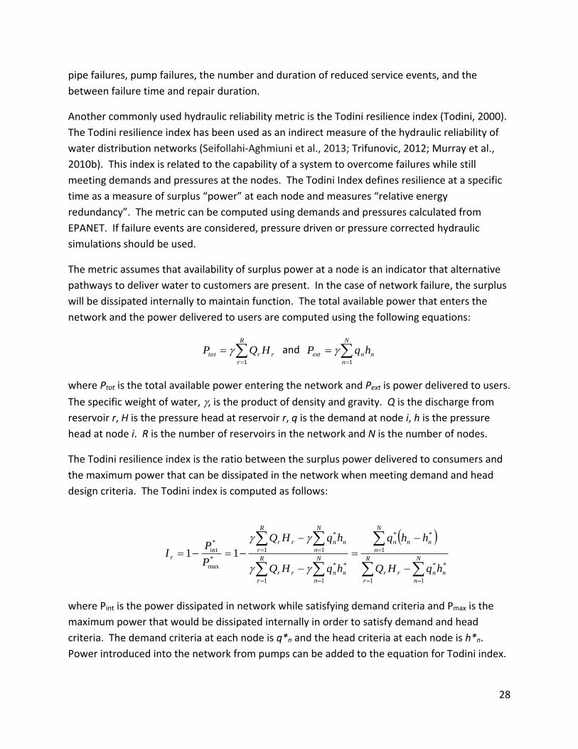
Another commonly used hydraulic reliability metric is the Todini resilience index (Todini, 2000).
The Todini resilience index has been used as an indirect measure of the hydraulic reliability of
water distribution networks (Seifollahi-Aghmiuni et al., 2013; Trifunovic, 2012; Murray et al.,
2010b). This index is related to the capability of a system to overcome failures while still
meeting demands and pressures at the nodes. The Todini Index defines resilience at a specific
time as a measure of surplus “power” at each node and measures “relative energy
redundancy”. The metric can be computed using demands and pressures calculated from
EPANET. If failure events are considered, pressure driven or pressure corrected hydraulic
simulations should be used.
The metric assumes that availability of surplus power at a node is an indicator that alternative
pathways to deliver water to customers are present. In the case of network failure, the surplus
will be dissipated internally to maintain function. The total available power that enters the
network and the power delivered to users are computed using the following equations:
R
r
rrtot HQP1
and
N
n
nnext hqP1
where Ptot is the total available power entering the network and Pext is power delivered to users.
The specific weight of water,, is the product of density and gravity. Q is the discharge from
reservoir r, H is the pressure head at reservoir r, q is the demand at node i, h is the pressure
head at node i. R is the number of reservoirs in the network and N is the number of nodes.
The Todini resilience index is the ratio between the surplus power delivered to consumers and
the maximum power that can be dissipated in the network when meeting demand and head
design criteria. The Todini index is computed as follows:
N
n
nn
R
r
rr
N
n
nnn
N
n
nn
R
r
rr
N
n
nn
R
r
rr
r
hqHQ
hhq
hqHQ
hqHQ
P
PI
1
**
1
1
**
1
**
1
1
*
1
*
max
*
int 11
where Pint is the power dissipated in network while satisfying demand criteria and Pmax is the
maximum power that would be dissipated internally in order to satisfy demand and head
criteria. The demand criteria at each node is q*n and the head criteria at each node is h*n.
Power introduced into the network from pumps can be added to the equation for Todini index.

29
Typically, the resilience index takes on values between 0 and 1, and higher values indicate
higher resilience.
Prasad and Park (2004) later modified the resilience index to add a weighting factor based on
the diameter of connecting pipes. The hydraulic reliability diagram is compared to the Todini
index and the weighted Todini index in Trifunovic (2012).
A related metric, the Todini failure index, can be used to evaluate and compare the effects of
pipe failures (Todini, 2000). While the resilience index allows some nodes with surplus power
to compensate for nodes with deficient power, the failure index highlights the nodes incapable
of providing enough power. The failure index is defined as follows:
***
*
1
**
1
:
: 0 where
nnnnn
nn
fnN
n
nn
N
n
fn
fhhihhq
hhiI
hq
I
I
A smaller failure index indicates better performance. Seifollahi-Aghmiuni et al. (2013) use the
failure index to evaluate network performance.
4.3.3 Entropy Reliability
The concept of entropy can be used as an indirect reliability metric to measure the number of
alternate paths between source and demand nodes in a water distribution network in the
presence of failed pipe(s). A network that carries maximum entropy flow is considered reliable
with multiple alternate paths. Awumah et al. (1990, 1991), Awumah and Goulter (1992), and
Tanyimboh and Templeman (1993, 2000) use entropy as a way to measure reliability in water
distribution networks.
These methods modify the standard entropy equations for use with water distribution
networks. A path parameter is added to count the number of independent paths from the
water source to the customer node at a specific time. The number of independent paths is less
than or equal to the total number of paths, which could be found using path enumeration.
Entropy can be computed using flows calculated from EPANET. If failure events are considered,
pressure driven or pressure corrected hydraulic simulations should be used. Entropy analysis
can be used to track how the number of redundant paths changes over a wide range of
hydraulic scenarios. Redundancy at any one node in the network depends on the redundancy
of upstream nodes. Flow reversal, especially in light of a link failure, also contributes to
redundancy of a node. This effect can be included in the entropy computation.
Awumah et al. (1990) define entropy using the following equation:

30
jj Lk jjk
jk
j
jk
Ui jij
ij
j
ij
jQa
q
Q
q
Qa
q
Q
qS lnln where
ijij MD
k
k
MD
k
kijij ddNDa11
11
Here, S’j is redundancy at node j, Uj is the set of nodes on the upstream ends of links connected
to node j, Lj is the set of outflow links connected to node j in which the link k belongs to a loop
containing j, qij is flow in link from node i to node j, Q’j is the total of all flow leaving and
entering node j, aij is the path parameter between nodes i and j, NDij is the number of
independent paths through the link from node i to demand node j, MDij is the number of links
in the NDij path, and dk is the number of paths in which link k is a member. Average network
entropy, S, is the average node redundancy over every demand node.
Maximizing average network entropy is equivalent to maximizing the ability of the network to
supply flow to each node (maximizing redundancy). Average network entropy has been
compared to node pair reliability (Quimpo and Shamsi, 1988) and percentage of demand
supplied at adequate pressure (PSPF) (Awumah and Goulter, 1989). Results from this
comparison show strong correlations, especially with PSPF. The authors note the relative ease
of computing entropy compared to PSPF, which requires hydraulic simulation for each pipe
removal. More recently, entropy and the resilience index were compared to exact calculations
of reliability and the resilience index was shown to be a more accurate indicator of reliability
than entropy (Creaco et al., 2014).
4.4 Standard Performance Measures
In water distribution systems analysis, additional common performance metrics include cost,
pressure, and water quality. Such metrics might also be useful when calculating resilience.
These metrics are defined below, and their relevance to evaluating resilience to hazards is
discussed.
4.4.1 Cost
Water utilities operate on tight budgets to build and maintain water distribution systems. For
that reason, cost is an important consideration when designing a new or retrofitting an existing
water distribution system. The Battle of Water Networks II (BWN-II), a network optimization
competition held at the Water Distribution Systems Analysis Conference in 2012, used cost,
along with water quality, and greenhouse gas emissions metrics, to evaluate the performance
of various network designs (Salomons, 2012). To evaluate cost, both the capital and
operational costs associated with any change to the system have to be considered. Capital
costs are related to purchases of new components and are dependent on the component size,
labor, transportation, and installation. Operational costs are related to the energy costs

31
associated with operating pumps and generators. Operational costs could also include
maintenance costs.
In Salomons, 2012, cost was calculated using the following equation:
C
c
cc OCCCCost1
where Cost is the total cost associated with system changes, CCc is the capital cost of new
component c and OCc is the operational cost for new component c. Some components, like
pipes, have no operational cost. BWN-II supplied capital and operational cost estimates for
network components. The capital cost of pipes and valves increases with diameter and the
capitol cost of tanks increases with volume. The operational cost of generators and pumps
increases with the desired power output. Both capital and operational costs are annualized to
reflect the total cost of maintenance and replacement associated with each component for one
year.
For many of the water distribution system hazards listed in Figure 2, cost would be an
important metric to use to account for upgrades required to enhance resilience to a given
hazard, or to repair the system following an event.
4.4.2 Water Quality
Another metric used to evaluate performance of water distribution networks is water quality.
Water quality was used to evaluate network design optimization in BWN-II (Salomons, 2012)
and by Murray et al. (2010a) to compare design and retrofit strategies. In both instances, water
age was used as a proxy for water quality. Water age is the time that a specific volume of water
is in the water distribution system after leaving the treatment plant or reservoir. Water utilities
try to minimize water age (also called residence time) as chlorine residuals are known to decay
and disinfection byproducts increase over time. EPANET has a built in function to calculate
water age at all nodes in the distribution system.
Murray et al. (2010b) compute the average water age in the network as follows:
N
n
T
t
ntANT
A1 1
1
where A is the average water age, Ant is the water age at junction n at time step t , N is the
number of junctions, and T is the number of time steps. Murray et al. (2010a) simulated water
quality under normal operating conditions over multiple days and averaged water age over the
last 24 hours in the water quality simulation to compute water age.

32
BWN-II uses a modified water age metric in which water age is only meaningful if it is above a
specified threshold that indicates potential water quality problems. Additionally, water age is
weighted by demand to reflect that high quality water is needed at customer service nodes. If
demand at a specific node and time is zero, then no water is consumed and water age at that
node-time pair is not used in the calculation. More weight is given to water age as demand
increases, which implies that the risk increases with consumption. Since water is not consumed
at tanks and reservoirs, water age at those junctions is not included in the calculation. For
BWN-II, average water age, weighted by demand, is computed as follows:
if 0
if 1 where
1 1
,
1 1
,
thnt
thnt
ijN
n
T
t
ntdem
N
n
T
t
ntntdemnt
AA
AAk
Q
AQk
A
where A is the average water age, Ant is the water age at junction n at time t ( tanks/reservoirs
excluded), Ath is a water age threshold which is used to set knt, Qdem,nt is the demand at junction
n and time step t, N is the number of junctions, and T is the number of time steps. For BWN-II,
Ath was set to 48 hours and the water quality simulation was run for 1 week on an hourly time
step. The water age metric was calculated over the entire simulation period and assessed
during normal system operations.
For many of the water distribution system hazards listed in Figure 2, water age might not be a
suitable metric. Water age would not capture changes in water quality due to contamination,
cross-connections, or system intrusions. Using EPANET, a water quality metric could calculate
chlorine residuals at each node in the network over time and report out the number of nodes
not meeting a minimum concentration threshold. Or, the fate and transport of specific
contaminants that enter the system could be modeled (e.g., total coliforms, hazardous release
agents). The systems measure could be the total quantity of the contaminant that enters the
system, or the number of hours the contaminant was present in the system. Both of these
approaches would require detailed knowledge about mechanisms within the distribution
system that affect the chlorine residual, for example, presence of biofilms on the pipe walls,
presence of natural organic matter in the bulk water, the type and age of pipe materials, and
the reaction kinetics of chlorine and specific contaminants. EPANET-MSX would be required to
calculate these new water quality metrics.
4.4.3 Water Pressure
Water distribution networks must maintain adequate water pressure throughout the network
to ensure continuity in service and for fire suppression. Low water pressure can result in flow
reductions and high water pressure can cause leaks and damage to system components. Water

33
pressures vary by communities, however, water pressure is typically maintained between 25
and 75 psi (Mays, 2000). Pressure is controlled in the network by pumps and the elevation of
reservoirs and tanks. Aside from pipe leaks and water consumption, pressure is lost in the
system due to pipe friction.
A systems analysis can be performed to ensure that a specific network meets pressure range
requirements under normal operating conditions and when the system is stressed by
component failure or changes to operations. EPANET can be used to calculate pressures at all
nodes in the system. The number of nodes that satisfy the pressure requirement over the
entire specified time period can be computed using the following equation:
otherwise 0
Tt1for P P if 1 where
L
1
Hnt
n
N
n
np
pkkN
where Np is number of nodes in the network that satisfy the pressure requirement, pnt is the
water pressure at junction n at time step t (tanks/reservoirs excluded), kn is a binary variable set
to 1 if the pressure requirement is satisfied at node n at time t, N is the number of junctions,
and T is the number of time steps. Similarly, the average percentage of nodes over the entire
specified time period that meet the pressure range requirement could be calculated.
Another important pressure measure indicates the ability of a system to provide an adequate
amount of pressure to fight fires. Under fire-fighting flows, large amounts of water are pulled
from a water distribution system; in residential areas, fire flows might range from 500-3,000
gallons per minute (gpm) while in commercial areas, fire flows might range from 2,500-10,000
gpm (Mays, 2000). The system must be able to maintain enough pressure to deliver the flow
rate needed to fight the fire. Typically, pressures must be above 20 psi at hydrants to deliver
adequate flow.
Murray et al. (2010b) measure the ability of the network to meet fire flow requirements as a
means to compare design and retrofit strategies. Networks were tested under a maximum day
demand pattern superimposed with a fire flow of 1,400 gpm. The number of nodes in each
network able to maintain pressures above 20 psi during firefighting was calculated as:
otherwise 0
ff wheref somefor ,tfor t psi 02 if 1 where
2121
1
ftpkkN
ntf
n
N
n
nF
where NF is the number of nodes that meet fire flow pressure requirements during the time
period of the fire flows, pntf is the water pressure at junction n at time step t for fire flow f, kn is
a binary variable that is set to 1 if the pressure at a specific node and time step meets fire flow

34
regulation, otherwise, kn is set equal to 0, t1 and t2 are the beginning and end of the firefighting
period, and f1 and f2 are the minimum and maximum flow rates.
For many of the water distribution system hazards listed in Figure 2, the pressure range
requirement might be a suitable metric. The concern would be that pipe breaks or other
system failures would result in pressures that are too low. The fire flow pressure metric might
be useful for measuring resilience to wildfires, earthquakes, and potentially chemical,
biological, radiological and nuclear (CBRN) attacks or other hazards.
4.5 Other Performance Metrics
Other systems metrics have been proposed for water distribution systems for various purposes,
and these might also be useful for measuring resilience. These metrics are defined below, and
their relevance to evaluating resilience to hazards is discussed.
4.5.1 Greenhouse Gas Emissions
The BWN-II competition used greenhouse gas (GHG) emissions as a metric to evaluate network
performance (Salomons, 2012). GHG emissions are important to consider given that water
utilities might need to adhere to regulations that limit emissions in the future. GHG emissions
are calculated by adding the capitol emissions associated with production, transport, and
installation of pipes, tanks, and pumps with the operational emissions resulting from fossil fuel
sources to operate pumps and generators. For BWN-II, GHG emissions is computed as follows:
C
c
cc OECE1
GHG
where GHG is the GHG emissions of the network, CEc is the capitol emissions from component c
and OEc is the operational emissions from component c. BWN-II supplied annualized CO2
equivalent emissions to manufacture specific pipes which shows that GHG emissions increase
with diameter. Operational GHG emissions is computed as the product of total annual pump
energy in the network and an emission factor of 1.04 kg-CO2-e/kWh. Just as with the cost
equation given in Section 4.4.1, some components have no operational cost. This metric is
particularly relevant to measuring resilience to climate change.
4.5.2 Water Security
Metrics that evaluate how a network performs in the event that contamination enters the
system have been used extensively to design sensor placement locations and response action
plans (Murray et al. 2010a, Murray et al. 2010b, USEPA, 2013b). Water security metrics can be
used to evaluate how potential contaminant incidents impact the population and the network.
The impact of contamination in a network depends on several factors, including the
contaminant type and strength, injection location and duration, fate and transport of the

35
contaminant, the dose and response to that dose by the population, the time needed to detect
and confirm contamination, and additional time needed to notify the public and implement
corrective actions. Based on this uncertainty, water security metrics should be evaluated using
an ensemble of possible contaminant scenarios and response times. Several water security
metrics can be computed using the Water Security Toolkit (WST) Impact Assessment Module
(USEPA, 2013b). These equations are summarized below. The water security metrics are
particularly useful for measuring resilience to hazards causing contamination of drinking water:
CBRN attacks and potentially floods, environmental emergencies, and others. The water
security metrics defined above can be cast as a measure of risk if the probability of individual
incidents is estimated.
4.5.2.1 Extent of Contamination
The extent of contamination, measured in length of contaminated pipe, for a particular
scenario when contaminant is detected by a sensor at time t’ is calculated using the following
equation:
th
I
i
N
n
CCLI
EC
int'
1 1
int' if 1
where EC is the average extent of contamination across the entire network for a set of
contamination incidents I when detected by a sensor at time ti’, Lint’ is the length of all pipes
starting at node n that are contaminated at the time of detection, Cint’ is the contaminant
concentration at node n at time ti’, and Cth is a contaminant threshold. N is the number of
junctions. An entire pipe is considered contaminated once the contaminant enters the pipe.
This metric is often used as a surrogate for the economic impacts of a contamination incident as
it indicates the length of pipe that will need to be cleaned or decontaminated.
4.5.2.2 Mass and Volume Consumed
The average mass of contaminant consumed in the network (i.e. the mass of contaminant that
leaves the water distribution network through customer demand nodes) and the average
volume of contaminant consumed (i.e., the volume of contaminant that leaves the network
through customer demand nodes) over a set of contamination incidents I when contaminant is
by a sensor at time ti’, is calculated using the following equations:
I
i
N
n
t
t
TqCI
MC1 1
'
1
intint
1
th
I
i
N
n
t
t
CCTqI
VC
int
1 1
'
1
int if 1

36
where MC is the average mass of contamination consumed across the entire network when
detected at a sensor at time ti’ and VC is the volume of contamination consumed across the
entire network when detected at a sensor at time ti’. Cint is the concentration of contaminant at
node n and time step t for incident i, qint is the demand at node n and time step t, and T is the
length of the time step. Cth is a contaminant threshold. N is the number of nodes, and T is the
number of time steps. Concentration is typically expressed in units of milligrams per Liter
(mg/L). This could also be a count of cells for a biological contaminant, where the units are
cells/L.
4.5.2.3 Time to Detection
The time to detection is the time from the beginning of a contamination scenario until the
contaminant is first detected at a sensor, averaged over all incidents, calculated by:
I
i
i TtI
TD1
'1
where ti’ is the time step when concentration is first detected and T is the length of the time
step. The scenario is not detected if the concentration never goes above a specified threshold.
4.5.2.4 Population Health Impacts
The population-based human health metrics require dose and response information for each
contaminant of interest. A disease progression model is used to predict the number of people
at each node susceptible to illness from the contaminant, exposed to a lethal or infectious dose,
experiencing symptoms of disease, and being fatally impacted. Population dosed (PD) is the
average number of individuals that received a cumulative dose of contaminant above a
specified threshold over a set of contamination scenarios I. Population exposed (PE) is the
average number of individuals exposed to harmful level of contaminant over a set of
contamination scenarios I. Population killed (PK) is the average number of individuals killed by
a contaminant over a set of contamination scenarios I. The equations for these health impacts
metrics are detailed in USEPA, 2013b.
4.5.3 Social Welfare Functions
Social welfare functions can be used to evaluate how well a water distribution network meets
the needs of its water customers or the community at large. Social welfare functions use
qualitative measures to evaluate a wide range of benefits to a society. To compute social
welfare functions, metrics have to be explicitly defined and data is collected using surveys or
through expert judgment. For example, social welfare functions can be used to measure the
perceived value of the water system to the community, or how much the water users are
willing to invest in infrastructure upgrades. Standard social welfare functions fall into one of
three categories: the utilitarian social welfare function, the Bergsonian social welfare function,

37
or the Rawlsian social welfare function. These functions differ in how stakeholders are
weighted. Amit and Ramachandran (2009) suggest the use of social welfare functions to
measure performance in water distribution networks. Hansen (2009) use social welfare
functions to determine water scarcity pricing to combat water shortages.
Milman and Short (2008) proposes a Water Provision Resilience (WPR) indicator to assess the
resilience of urban water systems. Their analysis estimates the ability of a water provider to
provide access to safe drinking water in the future. The WPR indicator uses a qualitative survey
of water utility experts to assess critical aspects of urban water system supply, infrastructure,
service population, water quality and governance.
These social welfare functions do not currently utilize systems analysis methodologies and are
therefore not recommended as resilience measures; however, some aspects of these
approaches could be incorporated into resilience systems measures.

38
5 Discussion While there is no single systems approach calculation to predict resilience of water distribution
systems to a wide range of hazards, a large number of performance metrics for water
distribution systems are available that might be helpful to quantitatively assess resilience to
hazards. While some of these metrics might only be useful for certain hazards, many of the
metrics could be useful for multiple types of hazards. It is important to note that none of these
performance metrics have been validated or tested against recent disasters to date.
Resilience measures: The time-based resilience measures are promising as they provide
detailed information about the benefits of resilience-enhancing actions. Such an approach
allows a user to explicitly calculate the effects of response and recovery actions or other
resilience-enhancing actions on all the system components and interactions. Much work is
needed to develop usable time-based resilience measures for WDS. Approaches to model
some response actions have already been developed (e.g., flushing hydrants, activating booster
stations), but new modeling approaches will need to be developed for other, more complex and
realistic actions. In the real world, response actions will include multiple actions at different
times, and modeling tools will need to be able to account for this. Other resilience enhancing
strategies might be undertaken in the mitigation phase rather than the response phase (e.g.,
decentralization of treatment and storage), and modeling tools need to be developed that can
simulate such actions. Hazard scenarios need to be developed to incorporate the effects of
natural disasters, terrorist attacks, and hazardous materials releases. Hydraulic and water
quality modeling software needs to be upgraded to more gracefully handle failures. Given the
range of possible response scenarios, multiple realizations of responses will need to be
simulated, perhaps using stochastic simulation approaches. Simulation software will need to be
improved to minimize computational time and memory usage, especially for large water
distribution system models.
Reliability measures: Currently, these are designed to measure the reliability of a WDS to pipe
failures by ensuring multiple flow paths. Some of the measures are indirect (e.g., topological
and Todini resilience index), while entropy is a direct calculation of flow paths. Some of the
methods also consider additional stresses on systems, such as maximum day demands or fire
flow conditions. As pipe breaks are a common outcome of many of the hazards listed in Figure
2, some of the reliability metrics, especially entropy, might prove to be useful. However, these
measures will need to be extended to additional stressor scenarios more representative of
conditions following a hazard (e.g., multiple pipe breaks throughout a WDS, failures of pumps
or valves, loss of access to storage tanks or sources). Stochastic simulation methods will need
to be developed to simulate these scenarios. To support the use of these reliability measures,
the simulation software will need to be extended to more gracefully handle failures by

39
continuing to produce results even under abnormal conditions. Separately, the topological
reliability metrics might be useful as a screening step, prior to more in-depth analyses.
Other measures: Cost is always an important metric that is needed in order to prioritize actions
and plan for expenditures. Cost information will need to be collected and updated on a regular
basis in order for this to be a useful metric. Water quality is critical to a water utility’s mission
and, therefore, this is an important measure to include to ensure that any resilience actions or
upgrades do not negatively impact water quality. Accurate water quality modeling can be
difficult as there is little data available from within WDS about biofilms, natural organic matter,
sediments, and other substances that interact with disinfectant residuals; improved water
quality models and data are needed to support this measure. The water security measures are
useful for understanding the effects of CBRN releases, other hazardous materials releases, and
other hazards that cause the release of contaminants into WDS. Some of the water security
measures require information about specific contaminants, their behavior in WDS, and their
health effects. Finally, GHG emissions is a useful measure for climate change scenarios.
In order to investigate the usefulness of each of these measures to calculating the resilience of
WDS to hazards, EPA and Sandia National Laboratories have partnered to develop a prototype
software tool to support resilience research. This tool uses water distribution network models
(in EPANET format) to compute a wide range of WDS performance metrics. The tool leverages
the EPANET toolkit (Rossman, 2000), third-party software designed to analyze and visualize the
structure of complex networks (Hagberg, 2008), and custom algorithms to compute resilience in
water distribution networks. This tool is being expanded to address some of the weaknesses in
WDS systems modeling tools described above. Ultimately, this tool is intended to support water
utilities, as a customizable way to investigate the resilience of their WDS to a wide range of
hazardous scenarios, and to evaluate resilience-enhancing actions.
Extensions to existing systems modeling approaches are necessary to enable analysis of all of
the hazards listed in Figure 2. Many of the hazards are likely to result in pipe breaks, causing an
abrupt change in flow patterns and pressures. EPANET is considered a “demand-driven” model,
but pressure-driven models and pressure-corrected models are available that might be better
suited to handle pipe breaks. With demand-driven simulation, customer water demand must
be met even if the pressure in the network decreases. When the demand condition cannot be
met, the simulation results are no longer meaningful. To get around this limitation, simulated
demand can be corrected based on a minimum pressure threshold (Wagner et al., 1988b) or
nodes can be changed to virtual tanks to supply demand when pressure is low (Trifunovic,
2012). Alternatively, pressure-driven simulation methods have been proposed. Pathirana
(2010) used an emitter based algorithm for pressure-driven simulations to develop an add-on
to EPANET. WaterNetGen also includes an EPANET extension for pressure driven analysis

40
(Muranho, 2012). Laucelli et al. (2012) compared the use of demand-driven and pressure-
driven simulation under different scenarios including climate uncertainty and asset
deterioration and conclude that pressure-driven simulation should be used to estimate the
hydraulic capacity of the network under these scenarios.
In addition, simulation tools need to be adapted to allow them to fail more gracefully; in other
words, rather than stopping a simulation when certain required demands or pressures cannot
be met, parts of the system could be allowed to fail, while other parts remain operational.
Additionally, models will need to be able to incorporate uncertainty in hazard scenarios and in
utility response strategies. Such changes and more will need to be made to water distribution
system models in order to allow for accurate modeling of hazardous events.
To summarize, systems modeling approaches need the following enhancements to adequately
address resilience of water systems to hazards:
Improvements to hydraulic and water quality software
o Ability to alter hydraulics mid simulation to better represent response scenarios
o Ability to compute reasonable results during abnormal operating conditions and
system failure
o Ability to support fast initialization from previous results, as well as “snap-shots”
from which a series of scenarios could be run
o Mathematical models of reaction dynamics for accurate water quality analysis
o Use of pressure driven or demand driven models when most appropriate
o Connections to field (SCADA) data to enable real time application of results
o Ability to propagate uncertainty through a single simulation (rather than
requiring separate scenario runs)
Improvements to network models
o Updated, validated utility network models to ensure accuracy and usability of
results
o Access to field (SCADA) data in order to improve model predictions
Improvements to model applications

41
o Set of scenarios to represent realistic disaster impacts and responses, including
pipe breaks, pump failures, power outages, control valve failures, insufficient
storage capacity, multiple stresses occurring at the same time, fire-fighting
conditions, and water quality failures
o Set of scenarios to represent realistic mitigation and response strategies that
water utilities might employ to reduce consequences of disasters
o Incorporation of uncertainty

42
6 Conclusions Resilience is a concept that is being used increasingly to refer to the capacity of infrastructure
systems to be prepared for and able to respond effectively and rapidly to hazardous events. In
Section 2 of this report, drinking water hazards, resilience literature, and available resilience
tools are presented. Broader definitions, attributes, and methods for measuring resilience are
presented in Section 3. In Section 4, quantitative systems performance measures for water
distribution systems are presented. Finally, in Section 5, the performance measures and their
relevance to measuring the resilience of water systems to hazards is discussed along with
needed improvements to water distribution system modeling tools.
Drinking water systems are subject to a range of hazards, from natural disasters to man-made
disasters such as terrorist attacks or hazardous material releases. The impacts of such events
on drinking water systems can include pipe breaks, service disruptions, power outages, loss of
public confidence, and more. Recent literature has focused on providing guidance to water
systems on increasing preparedness for disasters and guidance to planning for emergency
response and recovery. In addition, several tools have been developed for the water sector,
including the Community Based Water Resiliency (CBWR) tool and the Climate Resilience
Evaluation and Awareness Tool (CREAT). The Risk Analysis and Management for Critical Asset
Protection (RAMCAP) Standard for Risk and Resilience Management of Drinking Water and
Wastewater Systems presents an approach for measuring resilience. The Argonne National
Laboratory Resilience Index helps to measure resilience of water systems, but is intended to be
conducted by the Department of Homeland Security rather than being used as a self-
assessment tool.
Resilience is a broad concept and is used widely across many fields. Disaster resilience
incorporates many similar concepts such as reducing risk or vulnerability, enhancing
preparedness, and response; however, resilience differs from these concepts in that it also
includes the ability to effectively and rapidly recover from unforeseen events. Resilience is a
property of a system, and common attributes of resilient systems include redundancy,
robustness, rapid recovery, resourcefulness, and adaptability. Methods of measuring resilience
include developing a composite index incorporating diverse information from multiple fields or
using systems modeling approaches to explicitly calculate the effects of hazards on a system
and its interacting components. Systems modeling tools are available for water distribution
systems, and this report investigates their use.
Although there is not a single measure suitable for measuring the resilience of water systems to
hazards, multiple performance measures might be useful. Resilience measures include risk-
based qualitative approaches and systems-based quantitative approaches. Time-based
resilience measures simulate the system before, during, and after an event and allow for the

43
explicit evaluation of the impacts of resilience-enhancing actions. Reliability measures calculate
the ability of a water distribution system to meet pressure and flow requirements under normal
and emergency conditions, and fall into three categories: topological, hydraulic, and entropy-
based. Other performance measures, such as cost, water quality, and water security, are also
useful measures.
Finally, these measures are evaluated for their ability to inform resilience. In particular, the
time-based resilience measure, the entropy measure, cost, water quality, and water security
measures are likely to be effective. All of these measures, however, will require modifications
to existing systems analysis modeling tools in order to be used to inform resilience. New
scenarios need to be developed to allow for the explicit modeling of hazards and their effects
on water systems, especially natural disasters. Existing software, like EPANET, needs to be
modified to allow for failure of components in some parts of a system, while remaining
operational in other parts. These tools need to incorporate uncertainty inherent in the disaster
scenarios and in the utility response, using Monte Carlo or stochastic simulation approaches.
By enhancing systems-modeling tools and enabling network models to robustly handle failures
and stresses, a comprehensive evaluation of the benefits of each resilience metric can be
conducted, and improved resilience tools can be provided to the water sector.

44
References
ABAG Earthquake & Hazards Program. (2009). Water Systems and Disasters. San Fransico, CA:
ABAG Earthquake & Hazards Program.
Ajami NK, Truelove C. (2014). A water-energy research agenda: building California's policy
foundation for the 21st century. Stanford, CA: Water in the West, Stanford University.
Accessed September 19, 2014, http://waterinthewest.stanford.edu/sites/default/files/Water-
Energy%20Agenda-%20final-042514.pdf
American Water Works Association (AWWA), 2014. Process Control System Security Guidance
for the Water Sector. American Water Works Association.
Amit RK, Ramachandran P. (2009). Optimal design of water distribution networks: A review. The
Selected Works of R K Amit. Accessed September 19, 2014, http://works.bepress.com/rkamit/7
ANSI. (2010). Risk Analysis and Management for Critical Asset Protection (RAMCAP®) Standard
for Risk and Resilience Management of Water and Wastewater Systems, 2010, ANSI/ASME-
ITI/AWWA J-100-10.
ASCE. (2008). Recovery Practices Primer for Natural Disasters. Produced under the Water
Infrastructure Security Enhancements (WISE) Initiative by the American Society of Civil
Engineers (ASCE), American Water Works Association (AWWA), and the Water Environment
Foundation (WEF).
Attoh-Okine NO, Cooper AT, Mensah SA. (2009). Formulation of resilience index of urban
infrastructure using belief functions. IEEE Systems Journal, 3(2), pp. 147-153.
Awumah K, Goulter I, Bhatt SK. (1990). Assessment of reliability in water distribution networks
using entropy based measures. Stochastic Hydrology and Hydraulics, 4(4), 309-320
Awumah K, Goulter I. (1989). Redundancy and reliability of water distribution networks: An
entropy based approach. Presented at the 1989 National Conference on Hydraulic Engineering;
August 14-18, 1989, New Orleans, Louisiana, United States. In: Ports, M., ed., Proceedings of
1989 ASCE National Conference on Hydraulic Engineering, pp. 768-773.
Awumah K, Goulter I. (1992). Maximizing entropy defined reliability of water distribution
networks. Engineering Optimization, 20(1), 57-80.
Awumah K, Goulter IC, Bhatt SK. (1991). Entropy-based redundancy measures in water
distribution networks. Journal of Hydraulic Engineering, 117(5), 595-614.

45
Ayyub BM. (2013). System resilience for multihazard environments: Definitions, metrics, and
valuation for decision making. Risk Analysis, 34(2), 340-355.
Bao Y, Mays LW. (1990). Model for water distribution system reliability. Journal of Hydraulic
Engineering, 116(9), 1119–1137.
Barker K, Ramirez-Marquez JE, Rocco CM. (2013). Resilience-based network component
importance measures. Reliability Engineering and System Safety, 117, 89–97.
Berry J, Hart WE, Phillips CA, Uber JG, Watson JP. (2006). Sensor placement in municipal water
networks with temporal integer programming models. Journal of Water Resources Planning and
Management, 132(4), 218-224.
Berry J, Boman E, Riesen L, Hart WE, Phillips CA, Watson JP, and U.S. Environmental Protection
Agency. TEVA-SPOT Toolkit and user's manual- version 2.5.2. U.S. Environmental Protection
Agency, Washington, DC, EPA/600/R-08/041B, 2012.
Bloetscher F, Hammer N, Berry, L. (2014). How climate change will affect water utilities. Journal of the American Water Works Association, 106 (8): 176-192. CARRI. (2014). Community and Regional Resilience Institute. Accessed September 19, 2014, http://www.resilientus.org/about-us/what-is-community-resilience/ Chang SE. (2010). Urban disaster recovery: a measurement framework and its application to the 1995 Kobe earthquake. Disasters 34(2), 303-327.
CIPAC Workgroup. (2009). All Hazard Consequence Management Planning for the Water Sector. Produced by the Preparedness, Emergency Response, and Recovery CIPAC Workgroup of the Water Sector Critical Infrastructure Partnership Advisory Council (CIPAC). Accessed September 19, 2014, http://www.wef.org/uploadedFiles/Access_Water_Knowledge/Water_Security/Water_Security_PDFs/All-HazardCMPNovember2009FINAL.pdf
Concho Valley Council of Governments, Section 11 – Winter Storm. In: Hazard Mitigation Plan Update, 2012-2017, Concho Valley, Austin, TX: Concho Valley Council of Governments.
Creaco E, Fortunato A, Franchini M, and Mazzola, MR. (2014) Comparison between entropy and resilience as indirect measures of reliability in the framework of water distribution system design, Proceedings of the 12th International Conference on Computing and Control for the Water Industry (CCWI), Procedia Engineering 70(2014): 379-388.
Davis CA. (2013). Water System Seismic Resilience & Retrofit Strategies. In: Water Utility
Infrastructure Management Conference, July 17, 2013, Costa Mesa, CA.

46
DiGiano F, and Grayman W. (2014).Can we better protect vulnerable water supplies? JAWWA,
April 2014, 28-30.
Fiksel J. (2003). Designing resilient, sustainable systems. Environmental Science & Technology,
37(23), 5330-5339.
Fiksel J. (2006). Sustainability and Resilience: toward a systems approach. Sustainability:
Science, Practice, and Policy. Volume 2 (2): 14-21
Fiksel J, Goodman I, Hecht A. (2014) Resilience: Navigating a Sustainable Future. Solutions, Vol.
5, Issue 5, September/October 2014.
Fisher RE et al. (2010) Constructing a Resilience Index for the Enhanced Critical Infrastructure
Recovery Program. Lemont, IL: Argonne National Laboratory. ANL/DIS-10-9.
Francis R, Bekera B. (2013). A metric and frameworks for resilience analysis of engineered and
infrastructure systems. Reliability Engineering and System Safety, 121, 90-103.
FSIN. (2014). Resilience Measurement Principles: Toward an Agenda for Measurement Design.
World Food Program’s Food Security Information Network.
Fujiwara O, Ganesharajah T. (1993). Reliability assessment of water supply systems with storage
and distribution networks. Water Resources Research, 29(8), 2917-2924.
Gebhart BJ, Johnson S. (2014). The 500 Year Flood, One Year Later, Nine Lessons (Re)Learned.
Stormwater, July/August 2014.
Gilbert, SW. (2010). Disaster Resilience: A Guide to the Literature, NIST Special Publication
1117. Gaithersburg, MD: U. S. Department of Commerce, National Institute of Standards and
Technology (NIST).
Goulter I. (1987). Current and future use of systems analysis in water distribution networks
design. Civil Engineering Systems, 4(4), 175-184.
Grayman WM, Murray R, Savic DA. (2009). Effects of redesign of water systems for security and
water quality factors. In: Proceedings of the World Environmental and Water Resources
Congress 2009, Kansas City, MO, May 17-21, pp. 1-11.
Hagberg AA, Schult DA, Swart PJ. (2008). Exploring network structure, dynamics, and function using NetworkX. In: G Varoquaux, Vaught T, Millman J, eds., Proceedings of the 7th Python in Science Conference (SciPy2008), Pasadena, CA, August 19-24, pp. 11-15.
Hansen JK. (2009). Estimating impacts of water scarcity pricing. In: 27th International
Conference of the System Dynamics Society, July 26-30, 2009, Albuquerque, New Mexico.

47
Henry D, Ramirez-Marquez JE. (2012). Generic metrics and quantitative approaches for system
resilience as a function of time. Reliability Engineering and System Safety, 99, 114–122.
International Federation of Red Cross (IFRC). (2011). Characteristics of a Safe and Resilient
Community: Community Based Disaster Risk Reduction Study. 1224200 E 5/2012.
Jacobs P, Goulter I. (1988). Evaluation of methods for decomposition of water distribution
networks for reliability analysis. Civil Engineering Systems, 5(2), 58-64.
Jacobs P, Goulter I. (1989). Optimization of redundancy in water distribution networks using
graph theoretic principles. Engineering Optimization, 15(1), 71-82.
The Johnson Foundation. (2013). Building Resilient Utilities: How Water and Electric Utilities
Can Co-Create Their Futures. Racine, WI: The Johnson Foundation at Wingspread. Accessed on
September 19, 2014,
http://www.johnsonfdn.org/sites/default/files/reports_publications/CNW_ResilientUtilities.pdf
Lansey K. (2013). Sustainable, robust, resilient, water distribution systems. In: WDSA 2012: 14th
Water Distribution Systems Analysis Conference, Sept 24-27, 2012 in Adelaide, South Australia
1-18.
Laucelli D, Berardi L, Giustolisi O. (2012). Assessing climate change and asset deterioration
impacts on water distribution networks: Demand-driven or pressure-driven network modeling?
Environmental Modelling and Software, 37, 206-216.
Le Chevallier MW, Chelius JJ. (2014). Resiliency Planning Ensures Better Outcomes, Opflow,
40(1), 16-18.
Llanos M. (2011). 700 water main breaks in Houston - a day. Today – NBC News, 16 August
2011. [Online]. Accessed 6 June 2014, http://www.today.com/id/44160515/ns/today-
weather/t/water-main-breaks-houston-day/#.U57mtfldU1I.
Mays LW. (1996). Review of reliability analysis of water distribution systems. In: Xu IC, Tickle
KS, Wasimi S (eds.), Stochastic Hydraulics '96, Seventh IAHR International Symposium, Mackay,
Queensland, Australia, pp 53-62.
Mays LW. (1989). Reliability Analysis of Water Distribution Systems. Reston, VA: ASCE
Publications.
Mays LW. (2000). Water distribution systems handbook. New York: McGraw-Hill Professional.
McAllister T. (2013). Developing Guidelines and Standards for Disaster Resilience of the Built
Environment: A Research Needs Assessment, NIST TN 1795, 2013. Gaithersburg, MD: National

48
Institutes of Standards and Technology (NIST). Accessed on September 19, 2014,
http://www.nist.gov/manuscript-publication-search.cfm?pub_id=912299
Milman A, Short A. (2008). Incorporating resilience into sustainability indicators: An example for
the urban water sector. Global Environmental Change, 18(4), 758-767.
Muranho J, Ferreira A, Sousa J, Gomes A, Sá Marques A. (2012). WaterNetGen - an EPANET
extension for automatic water distribution networks models generation and pipe sizing. Water
Science and Technology: Water Supply, 12(1), 117-123.
Murray R, Haxton T, Janke R, Hart WE, Berry J, Phillips C. (2010a). Sensor network design for
drinking water contamination warning systems: A compendium of research results and case
studies using the TEVA-SPOT software. [Technical Report] Cincinnati, OH: U. S. Environmental
Protection Agency. EPA/600/R-09/141
Murray RE, Grayman WM, Savic DA, Farmani R. (2010b). Effects of DMA redesign on water
distribution system performance. In: Boxall J, Maksimovic C, eds., Proceedings of the 10th
International on Computing and Control for the Water Industry, CCWI 2009, University of
Sheffield, UK. CRC Press: Boca Raton, FL, pp. 645-650.
National Academy of Sciences (NAS). (2012). Disaster Resilience: A National Imperative,
prepared by the NAS Committee on Science, Engineering, and Public Policy. Washington, DC:
The National Academies Press.
National Infrastructure Advisory Council (NIAC). (2009). Critical Infrastructure Resilience, Final
Report and Recommendations, U.S. Department of Homeland Security, Washington, D.C.,
Accessed September 20, 2014.
http://www.dhs.gov/xlibrary/assets/niac/niac_critical_infrastructure_resilience.pdf.
Oregon Seismic Safety Policy Advisory Commission. (2013). The Oregon Reslience Plan:
Reducing and Improving Recovery for the Next Cascadia Earthquake and Tsunami. Salem, OR:
Oregon Seismic Safety Policy Advisory Commission.
Osnos, E. (2014). Chemical Valley: the coal industry, the politicians, and the big spill. The New
Yorker, April 7, 2014.
Ostfeld A, Kogan D, Shamir U. (2002). Reliability simulation of water distribution systems –
single and multiquality. Urban Water, 4, 53-61.
Ostfeld A. (2001). Reliability analysis of regional water distribution systems. Urban Water, 3(4),
253-260.

49
Ostfeld A. (2004). Reliability analysis of water distribution systems. Journal of Hydroinformatics,
6, 281-294.
Ozger SS. (2003). A semi-pressure-driven approach to reliability assessment of water
distribution networks, PhD Dissertation. Tempe, AZ: Department of Civil and Environmental
Engineering, Arizona State University.
Pandit A, Crittenden JC. (2012). Index for network resilience (INR) for urban water distribution
systems. 2012 Critical Infrastructure Symposium, Session 1A: Infrastructure Network Analysis.
April 23, 2012, Arlington, VA.
Pathirana A. (2011), EPANET2 Desktop Application for Pressure Driven Demand Modeling. In:
Lansey KE, Choi CY, Ostfeld A, Pepper I (eds.), Proceedings of the 12th Annual Conference of
Water Distribution System Analysis 2010 - WDSA2010, Sept. 12-15, Tucson, AZ.
Prasad TD, Park NS. (2004). Multiobjective genetic algorithms for design of water distribution
networks. Journal of Water Resources Planning and Management, 130(1), p 73–82.
Quimpo RG, Shamsi U. (1988). Network reliability for water distribution system management.
In: Proceedings of the 5th IAHR Symposium on Stochastic Hydraulics, University of Birmingham,
U.K, August 2-4.
Quimpo RG, Shamsi UM. (1991). Reliability based distribution system maintenance. Journal of
Water Resources Planning and Management, 117(3), 321–339.
Reed D, Stephenson R, Hyland S. (2013). Recovering from Hurricane Sandy: Coordination,
planning bolster storm response, Opflow, 39(5), 10-14.
Resilience Alliance. (2010). Assessing Resilience in Social-Ecological Systems: Workbook for
Practitioners. Version 2.0, 2010, Resilience Alliance.
Rossman LA. (2000). EPANET 2 Users Manual. [Technical report] Cincinnati, OH: U. S.
Environmental Protection Agency. EPA/600/R-00/057
Salomons E, Ostfeld A, Kapelan Z, Zecchin A, Marchi A, Simpson A. (2012). The battle of the
water networks II – Adelaide 2012 (BWN-II). In: Proceedings of the 2012 Water Distribution
Systems Analysis Conference, September 24-27, Adelaide, South Australia, Australia.
Scharfenaker M. (2006). Katrina stories highlight new realities of disaster planning, Journal of
the American Water Works Association, 98(6),16-30.

50
Seifollahi-Aghmiuni S, Bozorg Haddad O, Mariño MA. (2013). Water distribution network risk
analysis under simultaneous consumption and roughness uncertainties. Water Resources
Management, 27(7), 2595-2610.
Sewerage and Water Board of New Orleans. (2013). Katrina 8 Years Later, Progress, Recovery,
Restoration and Rebuilding. New Orleans: The Sewerage and Water Board of New Orleans.
Shamsi UM. (1990). Computerized evaluation of water-supply reliability. IEEE Transactions on
Reliability, 39(1), 35-41.
Shang F, Uber J, Rossman L. (2008). EPANET multi-species extension user’s manual. Technical Report. Cincinnati, OH: US Environmental Protection Agency. EPA/600/S-07/021
Shen Y, Vairavamoorthy K. (2005). Small world phenomena in water distribution network.
Computing in Civil Engineering, pp. 1-7.
Su YC, Mays LW, Duan N, Lansey KE. (1987). Reliability-based optimization model for water
distribution systems. Journal of Hydraulic Engineering, 113(12), 1539-1556.
Tanyimboh TT, Templeman AB. (1993). Maximum entropy flows for single-source networks.
Engineering Optimization, 22(1), 49-63.
Tanyimboh TT, Templeman AB. (2000). A quantified assessment of the relationship between
the reliability and entropy of water distribution systems. Engineering Optimization, 33(2), 179-
199.
Tierney K, Bruneau M. (2007). Conceptualizing and Measuring Resilience: A Key to Disaster Loss
Reduction. TR News, National Academies, Transportation Research Board, May-June 2007.
Todini E. (2000). Looped water distribution networks design using a resilience index based
heuristic approach. Urban Water, 2(2), 115-122.
Trifunovic N. (2012), Pattern Recognition for Reliability Assessment of Water Distribution
Networks, PhD Dissertation, Delft University of Technology, Delft, Netherlands.
UN-Water Taskforce on Water Security. (2013). Water Security and the Global Water Agenda:
A UN-Water Analytical Brief. Hamilton, Ontario, Canada: United Nations University, Institute for
Water, Environment & Health.
US Department of Energy. (2014). The Water Energy Nexus: Challenges and Opportunities. Washington, DC: U.S. Department of Energy. Accessed on September 19, 2014, http://energy.gov/sites/prod/files/2014/06/f16/Water%20Energy%20Nexus%20Report%20June%202014.pdf

51
US Environmental Protection Agency (USEPA). (2010). Water Contaminant Information Tool
(WCIT): A Robust Tool for the Water Sector. U. S. Environmental Protection Agency, Office of
Water: Washington, DC. EPA 817/F-10/016.
USEPA (2011). Community Based Water Resiliency Electronic Tool. U. S. Environmental
Protection Agency, Office of Water: Washington, DC. EPA 817/C-11/001. Accessed September
20, 2014, http://water.epa.gov/infrastructure/watersecurity/communities.
USEPA. (2012a). Climate Resilience Evaluation and Awareness Tool (CREAT). Washington, DC: U.
S. Environmental Protection Agency, Office of Water. Accessed September 19, 2014,
http://water.epa.gov/infrastructure/watersecurity/climate/creat.cfm
USEPA. (2012b). National Water Program 2012 Strategy: Response to Climate Change.
Washington, DC: U. S. Environmental Protection Agency, Office of Water.
USEPA. (2012c). CANARY User's Manual version 4.3.2. U.S. Environmental Protection Agency,
Washington, DC, EPA/600/R-08/040B, 2012.
USEPA. (2013a). Adaptation Strategies Guide for Water Utilities. Washington DC: U. S.
Environmental Protection Agency. EPA 817/K-13/001. Accessed September 19, 2014,
http://water.epa.gov/infrastructure/watersecurity/climate/upload/epa817k13001.pdf
USEPA. (2013b). Water Security Toolkit User Manual Version 1.1. [Technical Report].
Washington, DC: U.S. Environmental Protection Agency. EPA/600/R-13/353.
USEPA. (2013c). THREAT ENSEMBLE VULNERABILITY ASSESSMENT- SENSOR PLACEMENT
OPTIMIZATION TOOL (TEVA-SPOT) GRAPHICAL USER INTERFACE. (2013c). U.S. Environmental
Protection Agency, Washington, DC, EPA/600/R-13/014, 2013.
USEPA. (2014a). Planning for Flood Recovery and Long-Term Resilience in Vermont: Smart Growth Approaches for Disaster-Resilient Communities. Washington, DC: U. S. Environmental Protection Agency. EPA 231-R-14-003.
USEPA. (2014b). Water Security Home Website. U. S. Environmental Protection Agency.
Accessed September 19, 2014, http://water.epa.gov/infrastructure/watersecurity/index.cfm
USEPA (2014c). Flood Resilience: A Basic Guide for Water and Wastewater utilities.
Washington, DC: U. S. Environmental Protection Agency. EPA 817-B-14-006.
USEPA. (2014d). EPANET-RTX Libraries. EPANET-RTX 1.1. Accessed on September 20, 2014,
http://openwateranalytics.github.io/epanet-rtx/index.html,.

52
Vermont Agency of Natural Resources. (2011). Tropical Storm Irene by the Numbers. Accessed
Feb. 6, 2014, http://www.anr.state.vt.us/anr/climatechange/irenebythenumbers.html
Wagner JM, Shamir U, Marks DH. (1988a). Water distribution reliability: Analytical methods.
Journal of Water Resources Planning and Management, 114(3), 253-275.
Wagner JM, Shamir U, Marks DH. (1988b). Water distribution reliability: Simulation methods.
Journal of Water Resources Planning and Management, 114(3), 276-293.
WARN (Water/Wastewater Agency Response Network). (2013). Superstorm Sandy After-Action
Report. Denver, CO: American Water Works Association.
Watts DJ, Strogatz SH. (1998). Collective dynamics of 'small-world' networks. Nature, 393, 440-
442.
Welter, G. (2009). Natural disasters: Are you prepared? Opflow, 35(6), 12-16.
Yazdani, A. and Jeffrey, P. (2011). Complex network analysis of water distribution systems.
Chaos: An Interdisciplinary Journal of Nonlinear Science, 21(1), 016111.

Office of Research and Development (8101R) Washington, DC 20460
Official Business Penalty for Private Use $300
PRESORTED STANDARDPOSTAGE & FEES PAID
EPAPERMIT NO. G-35