Embed Size (px)
Citation preview
TU DELFT
System reliability analysis of belt
conveyor
by
Bart Zeeuw van der Laan
Supervised by: Dr. ir. X. Jiang
Transportation Engineering
March 2016

TU DELFT
Abstract
Supervised by: Dr. ir. X. Jiang
Transportation Engineering
by Bart Zeeuw van der Laan
This report is about the reliability of Belt Conveyor Systems. A literature search has
been conducted, about the working principles of sub-systems and components from the
belt conveyor system. Some general information about reliability is given. Later a
feasible state-of-the-art solution for improving the design of the belt conveyor system in
order to increase the overall reliability of the system.

Delft University of Technology
FACULTY OF MECHANICAL, MARITIME AND MATERIALS ENGINEERING Department of Marine and Transport Technology
Mekelweg 2 2628 CD Delft the Netherlands Phone +31 (0)15-2782889 Fax +31 (0)15-2781397 www.mtt.tudelft.nl
Student: Assignment type: Literature Supervisor: Dr.ir. Jiang Report number: 2015.TEL.xxxx Specialization: TEL Confidential: Creditpoints (EC): 10 Subject: System reliability analysis of belt conveyor As an important transportation equipment, belt conveyor has been widely applied in mining yards, harbor and airport etc. Typically, a belt conveyor consists of large numbers of components and subsystems; Moreover, the status of those components and subsystems would change with time and operation process. The complexity of both system and operation processes of a belt conveyor makes it very complicated and thus difficult to evaluate the safety and the reliability of a belt conveyor. In those regards, it is essential to introduce system reliability method to the design, evaluation and optimization of a belt conveyor in order to maintain its safety and operating process effectiveness. In this literature assignment, the student is demanded to review the development of system reliability method and its application on the design, evaluation, maintenance and optimization of belt conveyors. The following aspects are required to be illustrated in the report:
• Explain the basic theory of system reliability and available approaches /methods. • Identify the main components and subsystem of belt conveyer, their failure modes and
inter-relationship between those failure modes (dependent or independent; in series, or parallel or others. )
• Identify the main operation processes and their distribution in time domain; the status of components and subsystem with related to each operation process.
• Illustrate the state of the art: application of system reliability to design, evaluate, inspect and optimize belt conveyors.
This report should be arranged in such a way that all data is structurally presented in graphs, tables, and lists with belonging descriptions and explanations in text. The report should comply with the guidelines of the section. Details can be found on the website. If you would like to know more about the assignment, you may contact with Dr. X Jiang through [email protected]. The supervisor, X Jiang
Assignment v
-

Contents
Abstract iii
Assignment v
1 Introdcution 1
2 General reliability 3
2.1 General reliability . . . . . . . . . . . . . . . . . . . . . . . . . . . . . . . 3
Failure . . . . . . . . . . . . . . . . . . . . . . . . . . . . . . 4
Two state failure mode . . . . . . . . . . . . . . . . . . . . . 4
2.2 Failure rate . . . . . . . . . . . . . . . . . . . . . . . . . . . . . . . . . . . 4
Chance of failure . . . . . . . . . . . . . . . . . . . . . . . . 4
Cumulative failure distribution: . . . . . . . . . . . . . . . . 4
Survival rate: the probability that an item works until time T 4
Reliability function is the probability that the unit servesthe time interval t . . . . . . . . . . . . . . . . . 5
Failure rate: . . . . . . . . . . . . . . . . . . . . . . . . . . . 5
2.3 Life cycle . . . . . . . . . . . . . . . . . . . . . . . . . . . . . . . . . . . . 5
2.3.1 Infant mortality phase . . . . . . . . . . . . . . . . . . . . . . . . . 5
2.3.2 Normal life . . . . . . . . . . . . . . . . . . . . . . . . . . . . . . . 6
2.3.3 Wear out . . . . . . . . . . . . . . . . . . . . . . . . . . . . . . . . 6
2.3.4 Random overstress . . . . . . . . . . . . . . . . . . . . . . . . . . . 6
2.4 Multistate reliability . . . . . . . . . . . . . . . . . . . . . . . . . . . . . . 6
2.4.1 Failure rate data . . . . . . . . . . . . . . . . . . . . . . . . . . . . 7
2.4.2 Online and offline . . . . . . . . . . . . . . . . . . . . . . . . . . . 7
2.5 Systems . . . . . . . . . . . . . . . . . . . . . . . . . . . . . . . . . . . . . 7
2.5.1 Reliability Block diagram . . . . . . . . . . . . . . . . . . . . . . . 7
2.5.2 Interrelationships . . . . . . . . . . . . . . . . . . . . . . . . . . . . 8
Series . . . . . . . . . . . . . . . . . . . . . . . . . . . . . . 8
Parallel . . . . . . . . . . . . . . . . . . . . . . . . . . . . . 8
Combination of parallel and series . . . . . . . . . . . . . . 8
2.6 Redundancy . . . . . . . . . . . . . . . . . . . . . . . . . . . . . . . . . . . 9
2.7 FMEA . . . . . . . . . . . . . . . . . . . . . . . . . . . . . . . . . . . . . . 10
2.7.1 FMEA Failure mode and effects analysis . . . . . . . . . . . . . . . 10
2.7.2 Frequency/Consequence diagram . . . . . . . . . . . . . . . . . . . 10
2.8 Failure and failure modes . . . . . . . . . . . . . . . . . . . . . . . . . . . 10
vii
Contents viii
Cause of failure . . . . . . . . . . . . . . . . . . . . . . . . . 11
2.8.1 Failure modes . . . . . . . . . . . . . . . . . . . . . . . . . . . . . . 12
2.9 Markov Method . . . . . . . . . . . . . . . . . . . . . . . . . . . . . . . . . 12
2.10 Fault tree method . . . . . . . . . . . . . . . . . . . . . . . . . . . . . . . 13
2.11 Progressive reliability method . . . . . . . . . . . . . . . . . . . . . . . . . 14
2.12 Causal modeling theory . . . . . . . . . . . . . . . . . . . . . . . . . . . . 15
2.13 Bayesian Belief Network . . . . . . . . . . . . . . . . . . . . . . . . . . . . 15
Bayes rule: . . . . . . . . . . . . . . . . . . . . . . . . . . . 15
2.14 Fuzzy logic . . . . . . . . . . . . . . . . . . . . . . . . . . . . . . . . . . . 16
2.15 Historical data . . . . . . . . . . . . . . . . . . . . . . . . . . . . . . . . . 18
3 Components of Belt Conveyor Systems 19
3.1 Belt conveyor systems . . . . . . . . . . . . . . . . . . . . . . . . . . . . . 19
3.2 Definition . . . . . . . . . . . . . . . . . . . . . . . . . . . . . . . . . . . . 20
3.3 The system . . . . . . . . . . . . . . . . . . . . . . . . . . . . . . . . . . . 20
3.4 Components . . . . . . . . . . . . . . . . . . . . . . . . . . . . . . . . . . . 20
3.5 Belt . . . . . . . . . . . . . . . . . . . . . . . . . . . . . . . . . . . . . . . 20
3.5.1 Belt structure . . . . . . . . . . . . . . . . . . . . . . . . . . . . . . 21
3.5.2 Carcasses . . . . . . . . . . . . . . . . . . . . . . . . . . . . . . . . 21
3.5.3 Belt cover . . . . . . . . . . . . . . . . . . . . . . . . . . . . . . . . 22
3.6 Idlers . . . . . . . . . . . . . . . . . . . . . . . . . . . . . . . . . . . . . . 22
3.6.1 Idler structure . . . . . . . . . . . . . . . . . . . . . . . . . . . . . 22
3.6.2 Types of idlers . . . . . . . . . . . . . . . . . . . . . . . . . . . . . 22
3.6.3 Transition zone . . . . . . . . . . . . . . . . . . . . . . . . . . . . . 23
3.7 Pulleys . . . . . . . . . . . . . . . . . . . . . . . . . . . . . . . . . . . . . . 23
3.7.1 Drive pulley . . . . . . . . . . . . . . . . . . . . . . . . . . . . . . . 23
3.7.2 Drive pulley structure . . . . . . . . . . . . . . . . . . . . . . . . . 24
3.8 The drive unit . . . . . . . . . . . . . . . . . . . . . . . . . . . . . . . . . 24
3.8.1 Drive unit components . . . . . . . . . . . . . . . . . . . . . . . . . 24
3.8.2 Subsystems drive unit . . . . . . . . . . . . . . . . . . . . . . . . . 25
Motor . . . . . . . . . . . . . . . . . . . . . . . . . . . . . . 25
Coupling . . . . . . . . . . . . . . . . . . . . . . . . . . . . . 25
Gearbox . . . . . . . . . . . . . . . . . . . . . . . . . . . . . 25
Bearings . . . . . . . . . . . . . . . . . . . . . . . . . . . . . 25
3.9 Take-up system . . . . . . . . . . . . . . . . . . . . . . . . . . . . . . . . . 25
3.9.1 Transfer power . . . . . . . . . . . . . . . . . . . . . . . . . . . . . 26
Belt sag . . . . . . . . . . . . . . . . . . . . . . . . . . . . . 26
Tension . . . . . . . . . . . . . . . . . . . . . . . . . . . . . 26
3.9.2 Take-up system structure . . . . . . . . . . . . . . . . . . . . . . . 27
Types of take-up systems . . . . . . . . . . . . . . . . . . . 27
3.9.3 Gravity take-up system . . . . . . . . . . . . . . . . . . . . . . . . 27
3.9.4 Winch take up system . . . . . . . . . . . . . . . . . . . . . . . . . 27
3.9.5 Screw take up system . . . . . . . . . . . . . . . . . . . . . . . . . 28
3.10 Brake . . . . . . . . . . . . . . . . . . . . . . . . . . . . . . . . . . . . . . 29
3.10.1 Brakes . . . . . . . . . . . . . . . . . . . . . . . . . . . . . . . . . . 29
4 Belt conveyor failure modes 31
Contents ix
4.1 Schematic overview of the belt conveyor system . . . . . . . . . . . . . . . 31
4.1.1 Sub-systems . . . . . . . . . . . . . . . . . . . . . . . . . . . . . . . 31
4.1.2 The drive system . . . . . . . . . . . . . . . . . . . . . . . . . . . . 32
4.1.3 The belt . . . . . . . . . . . . . . . . . . . . . . . . . . . . . . . . . 32
4.1.4 The idlers . . . . . . . . . . . . . . . . . . . . . . . . . . . . . . . . 34
4.1.5 The take-up system . . . . . . . . . . . . . . . . . . . . . . . . . . 34
4.1.6 Brake system . . . . . . . . . . . . . . . . . . . . . . . . . . . . . . 35
4.2 Failure modes of belt conveyor system . . . . . . . . . . . . . . . . . . . . 35
4.2.1 Complete system . . . . . . . . . . . . . . . . . . . . . . . . . . . . 36
4.2.2 S1 Belt . . . . . . . . . . . . . . . . . . . . . . . . . . . . . . . . . 37
4.2.3 S2 Drive system . . . . . . . . . . . . . . . . . . . . . . . . . . . . 38
4.2.4 Failure mode of the idler system . . . . . . . . . . . . . . . . . . . 38
4.2.5 Failure mode of take up system . . . . . . . . . . . . . . . . . . . . 39
4.2.6 Failure mode of brake system . . . . . . . . . . . . . . . . . . . . . 39
5 Operation modes 41
5.1 Process states . . . . . . . . . . . . . . . . . . . . . . . . . . . . . . . . . . 41
5.2 Belt conveyor operation states . . . . . . . . . . . . . . . . . . . . . . . . . 41
5.3 Time distribution operational processes . . . . . . . . . . . . . . . . . . . 42
Normal operation . . . . . . . . . . . . . . . . . . . . . . . . 42
States . . . . . . . . . . . . . . . . . . . . . . . . . . . . . . 42
5.3.1 Steady state running z1 . . . . . . . . . . . . . . . . . . . . . . . . 43
5.3.2 Normal operational start z2 . . . . . . . . . . . . . . . . . . . . . . 43
5.3.3 Normal operational stop z4 . . . . . . . . . . . . . . . . . . . . . . 43
5.3.4 Emergency stop z5 and Aborted start z3 . . . . . . . . . . . . . . . 44
5.3.5 System at rest z6 . . . . . . . . . . . . . . . . . . . . . . . . . . . . 44
5.4 Fuzzy logic with Bayesian . . . . . . . . . . . . . . . . . . . . . . . . . . . 44
6 Automated reliability optimization 49
6.1 Conveyor belt system monitoring . . . . . . . . . . . . . . . . . . . . . . . 50
6.1.1 Automated belt conveyor monitoring . . . . . . . . . . . . . . . . . 50
6.1.2 Belt monitoring . . . . . . . . . . . . . . . . . . . . . . . . . . . . . 51
Belt interior monitoring . . . . . . . . . . . . . . . . . . . . 52
Belt surface monitoring . . . . . . . . . . . . . . . . . . . . 52
Speed monitoring . . . . . . . . . . . . . . . . . . . . . . . . 52
6.1.3 Force tension and torque measurement . . . . . . . . . . . . . . . . 53
6.1.4 Vibration monitoring . . . . . . . . . . . . . . . . . . . . . . . . . . 54
6.1.5 Power monitoring . . . . . . . . . . . . . . . . . . . . . . . . . . . . 54
6.1.6 Misalignment monitoring . . . . . . . . . . . . . . . . . . . . . . . 55
6.1.7 Temperature monitoring . . . . . . . . . . . . . . . . . . . . . . . . 55
6.2 Decision making . . . . . . . . . . . . . . . . . . . . . . . . . . . . . . . . 55
6.2.1 Artificial intelligence . . . . . . . . . . . . . . . . . . . . . . . . . . 57
6.2.2 Assessment for intelligent monitoring system . . . . . . . . . . . . 57
6.3 Reliability optimization . . . . . . . . . . . . . . . . . . . . . . . . . . . . 57
7 Conclusion 59
7.1 Recommendations . . . . . . . . . . . . . . . . . . . . . . . . . . . . . . . 60

Contents x
Bibliography 61
Chapter 1
Introdcution
Belt conveyor systems are used worldwide for multiple different options. They have been
around for about 250 years. Lodewijks [2014] Belt conveyor systems are in use and have
been used, for transporting people, bulk cargo and general cargo.
Belt conveyor systems are relatively complex systems used in heavy industry. They
contain of many rotating parts subject to wear. As in every industry the reliability of
systems is an important factor in the complete operation. Compared to other sectors
however relatively not that much reliability optimization has been done relating to the
operation and design of the system.
In sectors like the aircraft industry and offshore engineering a lot more research has been
done and the implantation of reliability centered maintenance is a lot further. By using
automated monitoring and decision systems predictive maintenance can be scheduled
instead of running the system until a random failure occurs.
In this report general reliability will be explained (Chapter 2) and the system of the belt
conveyor will be studied (Chapter 3). The different failure modes of the sub-systems
and components will be shown (Chapter 4) and the operation states are determined
(Chapter 5). Later possible modern options for the improvement of reliability of belt
conveyors will be shown (Chapter 6).
1
2
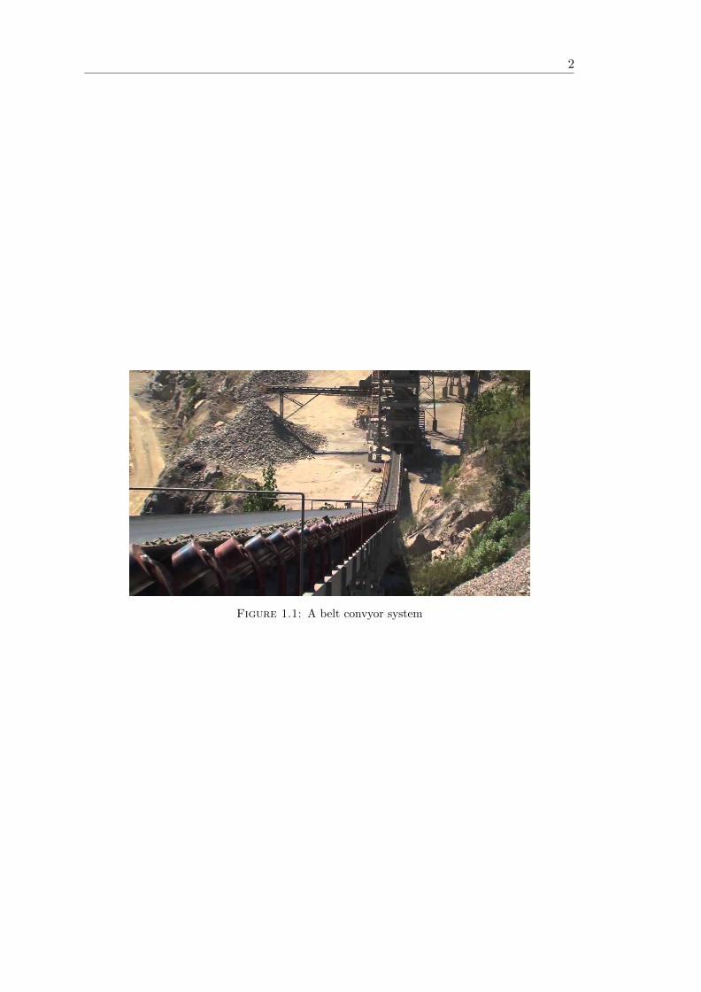
Figure 1.1: A belt convyor system

Chapter 2
General reliability
Over the years systems being used by mankind in all sectors of our society have become
more and more complex. By getting more and more complex these systems have become
a lot more advanced, but a good understanding of the reliability of the system has become
a lot harder. By the growing number of components and sub-system the cumulative
chance of one of these failing increased. Failing of one of these components or sub-
systems may cause the total system to fail. The total reliability became more and more
important. In order to get a better understanding for this, reliability engineering is used.
In the following section general reliability and failure are explained.
A system usually is a set of multiple subsystems. These sub-systems then can be made
up out of multiple different components. Failing of one of these components, may affect,
or lead to failure of the working of the entire system. Due to demands for cheaper safer
and highly reliable systems, for use in multiple different areas of work, two different
techniques for achieving high system reliability have been identified . Simply increasing
the strength or increasing the amount of backup solutions. The other technique for
improving the system reliability is a component reliability improvement program
2.1 General reliability
Reliability is about whether a system, sub-system or component will not fail. According
to accepted standards 1 failure is defined as ’the termination of the ability of an item to
perform a required function.’
3

4
Failure In general reliability theory a system, subsystem or component is either
working or not working. A component works until the moment it fails. This is usually
a function of time, but also other variables are possible.
Two state failure mode
X(t) =
{1 = component is working at time t
0 = component is not working at time t(2.1)
Failure modes According to British Standard BS 5760, Part 5, 3 failure mode is defined
as ’the effect by which a failure is observed on a failed item’.
2.2 Failure rate
The failure rate is the frequency with which an engineered system or component fails,
expressed in failures per unit of time. The failure rate of a system usually depends on
time, the rate varies over the life cycle of the component or system. In most cases the
failure rate is expressed in hours of use. Other possible options are to use distance or
revolutions etc. these can than replace the value of time. The failure rate is denoted by
λ.[Rausand, 1998]
Chance of failure f(t) is the chance a component fails on a certain time
Cumulative failure distribution:
F (t) =
t∫0
f(t) ∗ dt (2.2)
F (t) = 1−R(t) (2.3)
R(t) = 1− F (t) (2.4)
Survival rate: the probability that an item works until time T
F (t) = 1− e−λ∗t (2.5)
5
Reliability function is the probability that the unit serves the time interval
t
R(t) = e−λ∗t (2.6)
Failure rate:
r(t) =f(t)
R(T )(2.7)
2.3 Life cycle
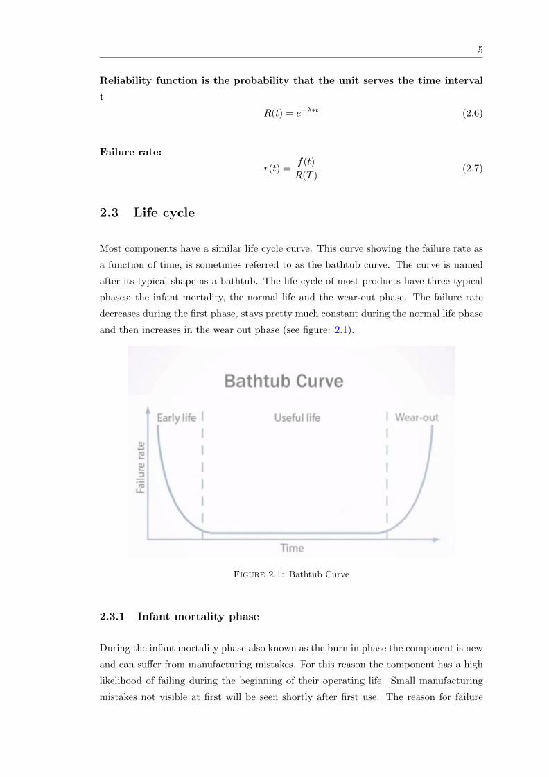
Most components have a similar life cycle curve. This curve showing the failure rate as
a function of time, is sometimes referred to as the bathtub curve. The curve is named
after its typical shape as a bathtub. The life cycle of most products have three typical
phases; the infant mortality, the normal life and the wear-out phase. The failure rate
decreases during the first phase, stays pretty much constant during the normal life phase
and then increases in the wear out phase (see figure: 2.1).
Figure 2.1: Bathtub Curve
2.3.1 Infant mortality phase
During the infant mortality phase also known as the burn in phase the component is new
and can suffer from manufacturing mistakes. For this reason the component has a high
likelihood of failing during the beginning of their operating life. Small manufacturing
mistakes not visible at first will be seen shortly after first use. The reason for failure
6
during this part of the operating process is mostly due to a mistake in manufacturing
or installation.
2.3.2 Normal life
After the burn in phase all the components with manufacturing or installation mistakes
are filtered out. The rate of failure usually then drops to a more constant lower level
where it will stay during its normal operating life. The component off course wears, but
is still able to fulfill its task. During this phase of the lifetime cycle there is still a chance
the component will fail but its lower and at a pretty much constant rate.
2.3.3 Wear out
Over time the component start to wear out more and more. Finally causing it to wear
out beyond proper use and or increasing the chance of direct failure. In this time of the
cycle the failure rate increases exponentially.
2.3.4 Random overstress
Except for usually regularly occurring patterns as the braking in phase and the wear
out; overstress is also an option of failure. During any time of the process its possible
that the component is put under a overstress causing it to fail.
2.4 Multistate reliability
For more complex system who age over time and its possible to introduce a multistate
analysis. [Yingkui and Jing, 2012] This allows to distinguish the overall reliability when
one or more components are aging. The amount of states is denoted by z. In the example
below z=3. [Rausand, 1998]
• a reliability state 3 the system operation is fully effective
• a reliability state 2 the system operation is less effective because of ageing
• a reliability state 1 the system operation is less effective because of ageing and
more dangerous for the environment
• a reliability state 0 the system is destroyed
7
2.4.1 Failure rate data
In order to better predict the failure of a component its possible to gather data about a
system or component. There are different ways of getting this data. The best and most
accurate one is testing the actual devices in order to generate failure data. Often this is
not completely possible and then instead historical data from similar systems is used.
2.4.2 Online and offline
To establish maintenance strategies and especially function testing strategies, it is im-
portant to distinguish between so-called evident and hidden failures. The following
classification of functions may therefore prove necessary:
1. On-line functions: These are functions operated either continuously or so often
that the user has current knowledge about their state. The termination of an
on-line function is called an evident failure.
2. Off-line functions: These are functions that are used intermittently or so infre-
quently that their availability is not known by the user without some special check
or test. An example of an off-line function is the essential function of an emer-
gency shutdown system. Many of the protective functions are off-fine functions.
The termination of the ability to perform an off-line function is called a hidden
failure.
[Rausand, 1998]
2.5 Systems
A system exists of multiple components working together. Therefore the working of the
system is depending on the working of the components. Depending on how the system
is build up failure of a certain component also lets the whole system fail or not. This
depends on the structure of the components in the system.
2.5.1 Reliability Block diagram
To retain the understanding of the functional interactions in the functional hierarchy,
and to clarify the required input and output interfaces, it is often useful to establish so-
called functional block diagrams. A block diagram is a clear way of modeling a system.
8
[Rausand and Ø ien, 1996] A block diagram contains of different blocks representing
components or sub-systems of the bigger system. The blocks are connected by lines
showing their relationship. For a system to work there must be a working route along
the blocks from the start till the end. If one of the component fails its not possible to
walk the route going over that block anymore.
2.5.2 Interrelationships
In a system components and subsystems can be in parallel or in series.
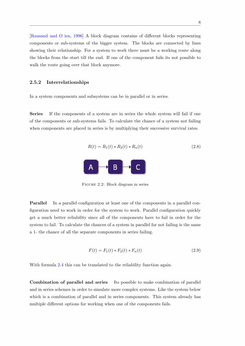
Series If the components of a system are in series the whole system will fail if one
of the components or sub-systems fails. To calculate the chance of a system not failing
when components are placed in series is by multiplying their successive survival rates.
R(t) = R1(t) ∗R2(t) ∗Rn(t) (2.8)
Figure 2.2: Block diagram in series
Parallel In a parallel configuration at least one of the components in a parallel con-
figuration need to work in order for the system to work. Parallel configuration quickly
get a much better reliability since all of the components have to fail in order for the
system to fail. To calculate the chances of a system in parallel for not failing is the same
a 1- the chance of all the separate components in series failing.
F (t) = F1(t) ∗ F2(t) ∗ Fn(t) (2.9)
With formula 2.4 this can be translated to the reliability function again.
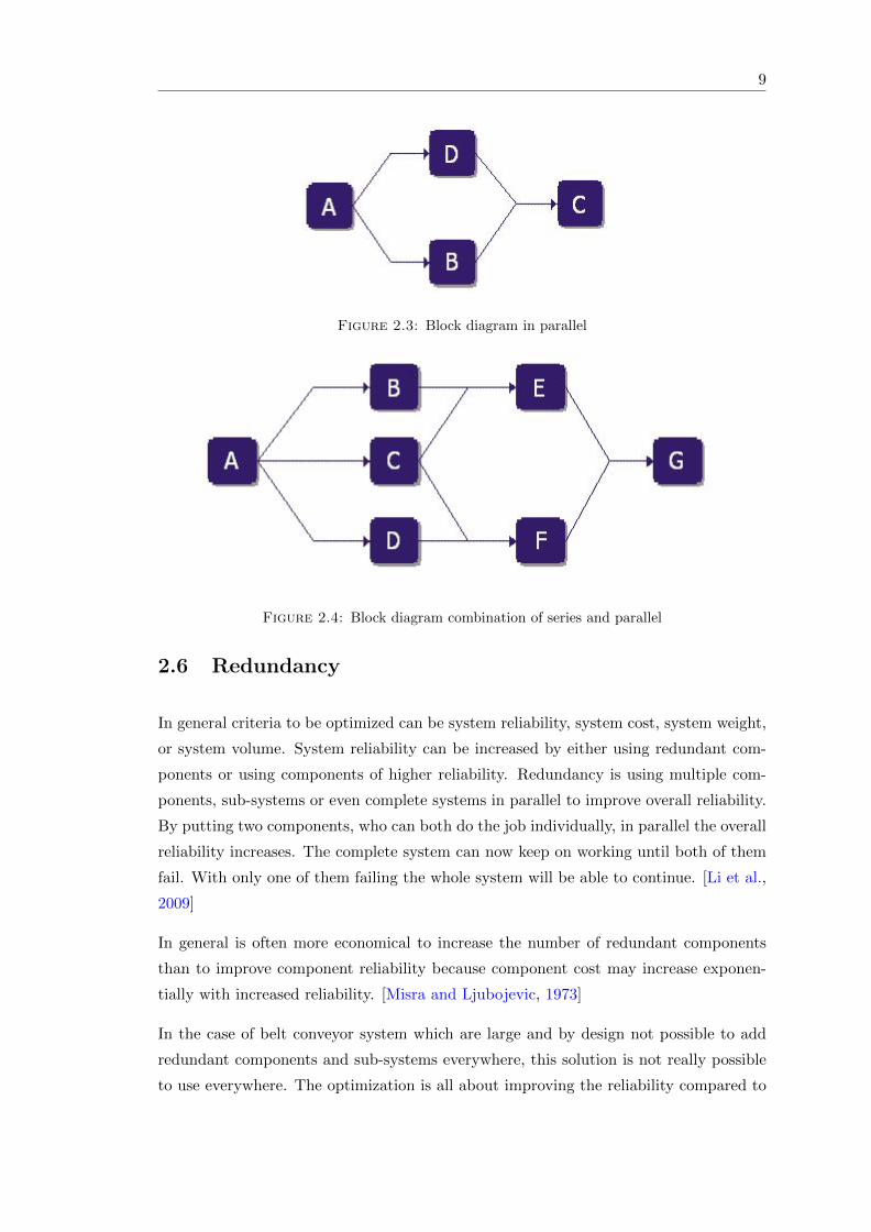
Combination of parallel and series Its possible to make combination of parallel
and in series schemes in order to simulate more complex systems. Like the system below
which is a combination of parallel and in series components. This system already has
multiple different options for working when one of the components fails.
9
Figure 2.3: Block diagram in parallel
Figure 2.4: Block diagram combination of series and parallel
2.6 Redundancy
In general criteria to be optimized can be system reliability, system cost, system weight,
or system volume. System reliability can be increased by either using redundant com-
ponents or using components of higher reliability. Redundancy is using multiple com-
ponents, sub-systems or even complete systems in parallel to improve overall reliability.
By putting two components, who can both do the job individually, in parallel the overall
reliability increases. The complete system can now keep on working until both of them
fail. With only one of them failing the whole system will be able to continue. [Li et al.,
2009]
In general is often more economical to increase the number of redundant components
than to improve component reliability because component cost may increase exponen-
tially with increased reliability. [Misra and Ljubojevic, 1973]
In the case of belt conveyor system which are large and by design not possible to add
redundant components and sub-systems everywhere, this solution is not really possible
to use everywhere. The optimization is all about improving the reliability compared to

10
the added costs. If the gains don’t out way the benefits it isn’t feasible. So for the design
of belt conveyors there is not so much to be gained using redundancy.
2.7 FMEA
2.7.1 FMEA Failure mode and effects analysis
The failure mode and effects analysis gives an overview of different components like-
lihood to fail and the consequences this may have. FMEA usually starts during the
early phases of system design and is performed by following the seven steps shown in
2.5. Some of the questions asked during the performance of FMEA with respect to
components/subsystems are as follows:
• What are the possible failure modes of the component/subsystem?
• What are the possible consequences of the failure mode?
• How is failure detected?
• How critical are the consequences?
• What are the effective safeguards against the failure in question?
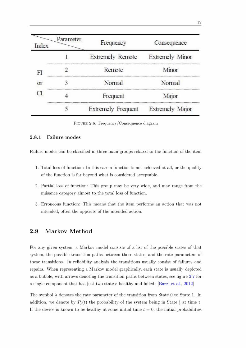
2.7.2 Frequency/Consequence diagram
In order to better understand and to give values to the frequency of different components
and systems failing they are sometimes categorised in a frequency/consequence diagram.
In this diagram all the different failure options are categorised by how likely they are to
occur and what the pairing consequence will be. The failure options are ranked with a
value from 1 to 5 for both the frequency as the severeness of the consequence. At this
way its easier to compare the different components with each other. Depending on the
type of the system the severeness of the consequences may vary and these need to be
established in order to make a fair comparison.
2.8 Failure and failure modes
Even if we are able to identify all the required functions of an item, we may not be able
to identify all the failure modes. This is because each function may have several failure
modes. No formal procedure seems to exist that may be used to identify and classify
the possible failure modes. Rausand and Ø ien [1996]

11
Figure 2.5: Steps for FMEA
A failure mode is a manifestation of the failure as seen from the outside. This means
the termination of one or more of its functions. Furthermore it’s important to make a
good distinction between the cause of failure and the failure mode itself.
Cause of failure Failure cause is ’the circumstances during design, manufacture or
use which have led to a failure This is what eventually causes a failure like for example
wear.
12
Figure 2.6: Frequency/Consequence diagram
2.8.1 Failure modes
Failure modes can be classified in three main groups related to the function of the item
1. Total loss of function: In this case a function is not achieved at all, or the quality
of the function is far beyond what is considered acceptable.
2. Partial loss of function: This group may be very wide, and may range from the
nuisance category almost to the total loss of function.
3. Erroneous function: This means that the item performs an action that was not
intended, often the opposite of the intended action.
2.9 Markov Method
For any given system, a Markov model consists of a list of the possible states of that
system, the possible transition paths between those states, and the rate parameters of
those transitions. In reliability analysis the transitions usually consist of failures and
repairs. When representing a Markov model graphically, each state is usually depicted
as a bubble, with arrows denoting the transition paths between states, see figure 2.7 for
a single component that has just two states: healthy and failed. [Bazzi et al., 2012]
The symbol λ denotes the rate parameter of the transition from State 0 to State 1. In
addition, we denote by Pj(t) the probability of the system being in State j at time t.
If the device is known to be healthy at some initial time t = 0, the initial probabilities

13
Figure 2.7: Markov states
of the two states are P0(0) = 1 and P1(0) = 0. Thereafter the probability of State 0
decreases at the constant rate λ, which means that if the system is in State 0 at any
given time, the probability of making the transition to State 1 during the next increment
of time dt is λ ∗ dt.
dP0 = −(P0) ∗ (λ ∗ dt) (2.10)
2.10 Fault tree method
Another widely used method is the Fault tree method. It uses different kind of blocks
to show the types of linkages. Figure 2.8 shows the four most commonly used blocks in
fault trees. [Dhillon, 1989] The Fault tree method, makes a better understanding of the
system. With analyzing tools and optimization the reliability can than be improved.
Figure 2.8: Most common used blocks
The fault tree is structured using the following steps: see figure 2.9

14
Figure 2.9: Steps for making a Fault tree
2.11 Progressive reliability method
A progressive reliability method calculates the failure probability of a structural system
accounting for the progressive failure of system components until the system fails. In
this method, two important terminologies are essential and frequently referred to, which
are (a) a configuration and (b) a failure scenario.
We define a configuration as any possible state of the structure in terms of the possible
state (failure or no failure) of its components. This definition is based on the assumption
that any component may fail and is always either in the state of failed or in the state
of not failed. Any structural system has an initial arrangement of its components. We
call the initial state of a structural system (with no failed components) as the intact
configuration. Under the effect of environmental loads, some components may fail. Any
component failure leads the system to a new configuration. If a system has N components
that may potentially fail, the total number of possible configurations is 2N .
We define a failure scenario of Xi as a group of steps (or the path) that leads the
system from X0 (the intact configuration) to Xi. In general, the occurrence of Xi can
be through one or more failure scenarios. However, because in a structural system,
the environmental loads usually vary within a time frame until reaching to a maximum
load, and that the capacity of the components are random, it is almost impossible that
in more than one component, the internal force exceed the capacity at the same time.
Therefore we assume that one component fails at a time. [Mousavi et al., 2013]

15
The method is best explained with an example of two beams being able to withstand a
force when they work in pairs. When one of them breaks the other will follow since it
won’t be able to withstand the force by itself.
2.12 Causal modeling theory
Causal modeling theories provide the user intuitive and mathematically sound tools
to model complex relations between uncertain variables and failure causes. The de-
velopment of causal modeling is resulting in the development of new diagnostic and
decision-making methodologies in field of large-scale conveyor belt systems. Pang and
Lodewijks [2006]
However, not all modeling methodologies can fully match the requirements of practical
conveyor belt systems maintenance decision- making. The Bayesian method compared
to the other methodologies has the advantage of handling both discrete and continuous
events and reasoning with partial or limited information. [Pang and Lodewijks, 2006]
The Bayesian Belief Network method is explained in the next section.
2.13 Bayesian Belief Network
Bayesian Belief Networks are based on the Bayesian method. The method is a mean to
calculate the likelihood of a future event based on the frequency the event has occurred
in the past.
Bayes rule:
P (A|B) =P (B|A) ∗ P (A)
P (B)(2.11)
P (A) is the prior probability of the likelihood of event A. The event A is considered as
independent from other events and the probability doesn’t take into account information
about other events. P (B) is the prior probability of the likelihood of event B. The
event B is considered as independent from other events and the probability doesn’t
take into account information about other events. P (B|A) is the probability that B
occurs given that A occurs. It is the posterior probability of event A, which is derived
from the specified value of event B. The rule shows the condition between two reverse
probabilities.
16
Bayes rule allows to gain posterior knowledge by using prior knowledge to calculate the
probabilities of other events. Bayesian interference is therefore used to see the cause
effect relationships between evidence and hypothesis. [Langseth and Portinale, 2007]
The Bayesian method can be used in two ways. It can either be used forward and
backward. In the forward interference the effects are derived from the causes. This will
enable prediction of events. Knowing that components have worn out will lead to less
well operation. With the backward interference the causes are derived from the effects.
By observing poor operation it can be derived that components are wearing out.
The method can be used to determine the cause-effect relationship between evidence
and hypothesis. The posterior probability P (E|H) of an event or evidence (E) can be
can be derived with the observed hypothesis (H). This can be used to identify the cause
of an event. This is called the backward interference. It can also be used the other way
around P (H|E) to discover the effect of an event. This is called the forward Bayesian
interference. [Langseth and Portinale, 2007]
The rule shows that the hypothesis is closer to the truth by means of the events that
have been observed. Considering multiple events the rule expressed as:
P (ei|H) =P (H|ei) ∗ P (ei)∑i P (H|ei) ∗ P (ei)
(2.12)
The prior knowledge P (ei) of a set of events ei(i = 1, 2, 3, ..., n) is used to find out the
posterior knowledge of P (ei) of the set of events given hypothesis H.
A Bayesian Belief Network is a network with on the nodes the probabilistic functions
and connecting the relationships. In automated networks new data is used to update all
the possible events.
The belt conveyor system has a lot of components which can not be measured directly
but the effects can be measured. By combining all the effects and using a Bayesian
Belief Network new inside can be given about the state of components which otherwise
would’ve been hard to notice.
2.14 Fuzzy logic
In order to transform the data measured to more quantified data to be used in automated
systems. Fuzzly logic is used to transform the fuzzy data to be more easily used. [Zadeh,
1983]
17
According to [Lodewijks, 2014] there are five reasons to use fuzzy logic as a tool to use
on the data for the conveyor belt system.
• It allows interpretations of more fuzzy observations
• It increases the consistency of the inspection if the observations are done by dif-
ferent interpreters.
• It allows to combine the inspection data to be combined with other source infor-
mation.
• It allows objectification of the results
• It gives a straightforward advice
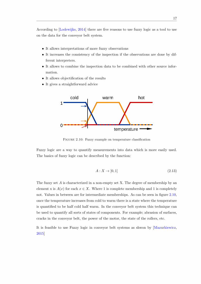
Figure 2.10: Fuzzy example on temperature classification
Fuzzy logic are a way to quantify measurements into data which is more easily used.
The basics of fuzzy logic can be described by the function:
A : X → [0, 1] (2.13)
The fuzzy set A is characterized in a non-empty set X. The degree of membership by an
element x is A(x) for each x ∈ X. Where 1 is complete membership and 1 is completely
not. Values in between are for intermediate memberships. As can be seen in figure 2.10,
once the temperature increases from cold to warm there is a state where the temperature
is quantified to be half cold half warm. In the conveyor belt system this technique can
be used to quantify all sorts of states of components. For example; abrasion of surfaces,
cracks in the conveyor belt, the power of the motor, the state of the rollers, etc.
It is feasible to use Fuzzy logic in conveyor belt systems as shwon by [Mazurkiewicz,
2015]

18
2.15 Historical data
In order to have the reliability values of components real data of the working components
gives the best values. In order not having to test every single component over a complete
lifespan a database could be used. This kind of databases have proven to be a well work-
ing extra in comparing the values measured from a system and making better decisions.
In the offshore sector OREDA has been a proven example of a system which has been
in use trough multiple offshore operators. Rausand [1998] The OREDA database covers
a very large amount of components used in systems by different offshore operators. The
data allows other companies to gain knowledge about the failure rates and lifetime ex-
pectancies of components. Especially for the components who have longer lifetime and
where testing would be a very costly exercise, this gathered information from the same
component also used in the field could be very beneficial.
Chapter 3
Components of Belt Conveyor
Systems
Belt conveyors systems are commonly used systems for continuous transport, they have
a high efficiency, large conveying capacity, relatively simple construction and relatively
small amount of maintenance. In the next part the different components and subsys-
tems of the belt conveyor system will be explained. From these different systems and
subsystems the failure modes and interrelationships between these failure modes will be
explained.
3.1 Belt conveyor systems
Belt conveyor systems are used worldwide for multiple different options. They have
been around for about 250 years. Lodewijks [2014] Belt conveyor systems are in use and
have been used, for transporting people, bulk cargo and general cargo. In this report
the focus will be on belt conveyors for bulk cargo. These belt conveyor systems play
an important role in the mining industry, bulk terminals, power plants, and chemical
production. Belt conveyor systems can be used in places where the terrain is rough and
where there is no current infrastructure of roads or railroads. Belt conveyor systems will
then be a highly efficient way of continuously moving bulk material fast. Fedorko et al.
[2013]
19
20
3.2 Definition
A belt conveyor is a continuous conveyor that consists of two or more pulleys, with a
continuous loop of material - the conveyor belt - that rotates about them. At least one
of the pulleys is powered, moving the belt and the load on the belt forward.
3.3 The system
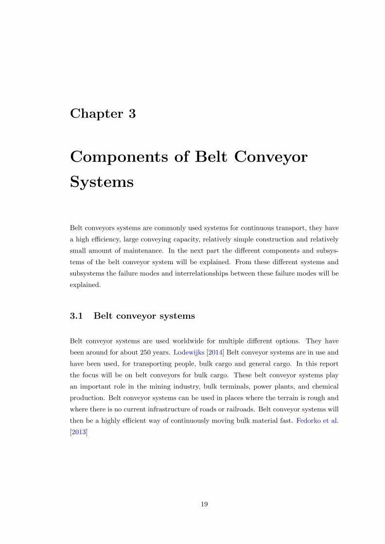
The belt conveyor system consists of different components. The major components are:
the belt, pulleys, idlers, take-up system, drive unit and sometimes the brakes. A belt
conveyor system is always being used in a bigger system. For this report the focus is on
the belt conveyor itself therefore leaving out the different parts of the complete system.
For example the loading hopper is not being taken into account in this report. The
different systems containing of subsystems which will be shown later in the report.
Figure 3.1: A Belt Conveyor System
3.4 Components
3.5 Belt
The belt is the major component of a belt conveyor system. It is constantly moving
around with the transporting good on top. The bulk material should have a relative
speed of zero compared to the belt itself.

21
3.5.1 Belt structure
The belt consists of two main components: its carcass and belt covers. The carcass of the
belt is to transfer the power of the drive force running through the belt and the lateral
forces. The required strength of the carcass is a function of the maximum force inside
the belt and the belt width. The belts should be made of a strong yet flexible material.
The costs of the belt can make up to half of the price of the whole BCS. On the sides
is a protective edge to protect the inner structure from being damaged. The bottom
and top have a covering layer. The functions of this covers is to protect the expensive
carcass. Figure 3.2 shows a schematic drawing showing the different components of the
belt.
Figure 3.2: Structure of a conveyor belt
3.5.2 Carcasses
As mentioned earlier the carcass needs to be strong in order to withstand the forces
running through the belt. Furthermore the carcass needs to be flexible in order to be
able to follow the path of the system. Two options for the construction of the carcass
are a fabric or a steel cord carcass. Mazurkiewicz [2008]
Figure 3.3: A Belt with steel cables
22
3.5.3 Belt cover
Depending on the field of use the belt cover needs to have specific qualities. Overall it
needs to be durable and it needs to be able to protect the expensive carcass. Possible
other qualities are:
• Anti-static
• Fire resistant
• Cold resistant
• Oil resistant
3.6 Idlers
The idlers are used to support the belt. They are a set of rolls where the belt runs upon.
Depending on the length of the system and the weight of the load a system may have
more or less idlers. In a bulk BCS its possible to use angled idlers next to each other in
order to make up trough for a better form for the transportation of the bulk.
3.6.1 Idler structure
An idler consists of a frame, rolls and bearings. The belt rolls over the rolls. The
bearings are used to make the roll turn smooth. The bearings are fitted on the sides of
the rolls. Since idlers can break and the system usually contains of a lot of idlers they
should be easily replaceable.
3.6.2 Types of idlers
Belt conveyor systems have a large amount of idlers, these can be divided up into four
different types:
• trough roller
• parallel roller
• buffer roller
• self alligning roller
These can be divided into no-load and load bearing idlers. Zhao and Lin [2011]
23
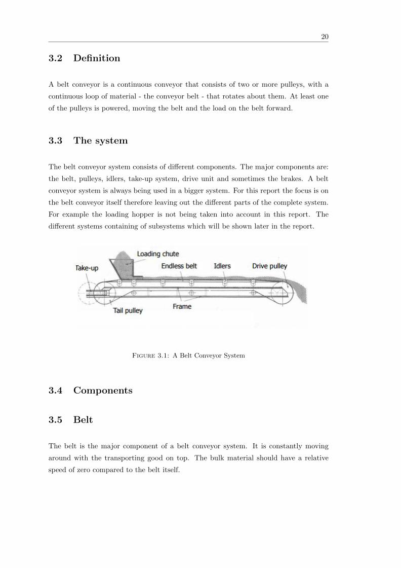
3.6.3 Transition zone
The drive pulley is just one big roll therefore having the belt to pass it completely flat.
If a trough shape for the rest of the belt trajectory is required a transition zone is made
up from idlers going into a more inclined angle gradually. The length required to go
from a flat belt to the desired trough shape is called the transition distance. Alspaugh
[2004]
Figure 3.4: Transition zone
3.7 Pulleys
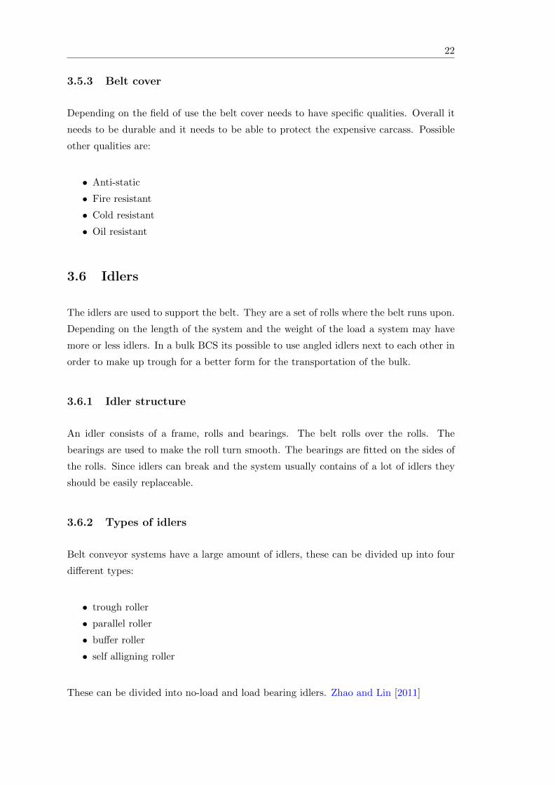
3.7.1 Drive pulley
In most cases the belt needs a form of active propulsion in order for the system to start
and keep in motion. This active form of propulsion is needed to overcome the friction
forces, moment of inertia and possible positive gravity forces. The drive pulley is a
roller who is propelled and transforms power to the belt. The drive pulley converts the
rotational speed of the drive pulley into a longitudinal speed of the belt. HOU and
MENG [2008]
Figure 3.5: Drive pulley overview
24
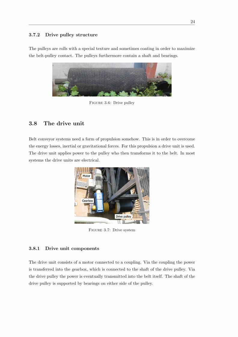
3.7.2 Drive pulley structure
The pulleys are rolls with a special texture and sometimes coating in order to maximize
the belt-pulley contact. The pulleys furthermore contain a shaft and bearings.
Figure 3.6: Drive pulley
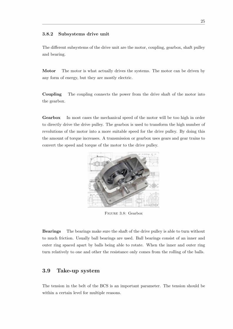
3.8 The drive unit
Belt conveyor systems need a form of propulsion somehow. This is in order to overcome
the energy losses, inertial or gravitational forces. For this propulsion a drive unit is used.
The drive unit applies power to the pulley who then transforms it to the belt. In most
systems the drive units are electrical.
Figure 3.7: Drive system
3.8.1 Drive unit components
The drive unit consists of a motor connected to a coupling. Via the coupling the power
is transferred into the gearbox, which is connected to the shaft of the drive pulley. Via
the drive pulley the power is eventually transmitted into the belt itself. The shaft of the
drive pulley is supported by bearings on either side of the pulley.
25
3.8.2 Subsystems drive unit
The different subsystems of the drive unit are the motor, coupling, gearbox, shaft pulley
and bearing.
Motor The motor is what actually drives the systems. The motor can be driven by
any form of energy, but they are mostly electric.
Coupling The coupling connects the power from the drive shaft of the motor into
the gearbox.
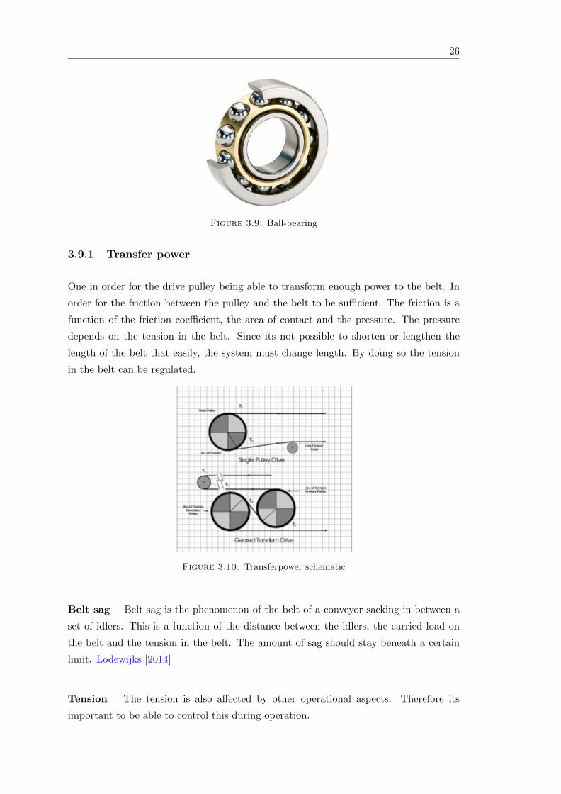
Gearbox In most cases the mechanical speed of the motor will be too high in order
to directly drive the drive pulley. The gearbox is used to transform the high number of
revolutions of the motor into a more suitable speed for the drive pulley. By doing this
the amount of torque increases. A transmission or gearbox uses gears and gear trains to
convert the speed and torque of the motor to the drive pulley.
Figure 3.8: Gearbox
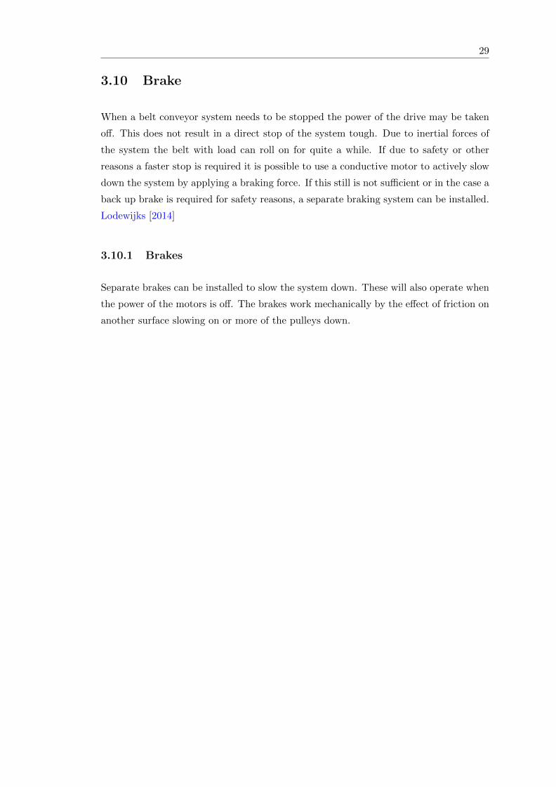
Bearings The bearings make sure the shaft of the drive pulley is able to turn without
to much friction. Usually ball bearings are used. Ball bearings consist of an inner and
outer ring spaced apart by balls being able to rotate. When the inner and outer ring
turn relatively to one and other the resistance only comes from the rolling of the balls.
3.9 Take-up system
The tension in the belt of the BCS is an important parameter. The tension should be
within a certain level for multiple reasons.
26
Figure 3.9: Ball-bearing
3.9.1 Transfer power
One in order for the drive pulley being able to transform enough power to the belt. In
order for the friction between the pulley and the belt to be sufficient. The friction is a
function of the friction coefficient, the area of contact and the pressure. The pressure
depends on the tension in the belt. Since its not possible to shorten or lengthen the
length of the belt that easily, the system must change length. By doing so the tension
in the belt can be regulated.
Figure 3.10: Transferpower schematic
Belt sag Belt sag is the phenomenon of the belt of a conveyor sacking in between a
set of idlers. This is a function of the distance between the idlers, the carried load on
the belt and the tension in the belt. The amount of sag should stay beneath a certain
limit. Lodewijks [2014]
Tension The tension is also affected by other operational aspects. Therefore its
important to be able to control this during operation.

27
Figure 3.11: Belt sag
3.9.2 Take-up system structure
There are different type of options for a take-up system, but they all have in common
that a pulley is used in order to exert a force on the belt in the outward direction of
the system. In this way lengthening it, in order to increase the tension in the belt.
Lodewijks [2014]
Types of take-up systems There are three mayor types of take-up systems:
1. Gravity take-up system
2. Winch take-up system
3. Screw take-up system
3.9.3 Gravity take-up system
The gravity take-up system makes use of gravity in order to put the proper amount of
tension on the belt. The working principle is a set of pulleys and a weight thats forced
down by gravity in order to put tension on the belt. A system likes this varies the
length of the belt in the system in order to keep the belt tension constant throughout
operation.
3.9.4 Winch take up system
A winch take up system makes use of a winch to vary the length of the belt in the
system, keeping the tension constant throughout operations.

28
Figure 3.12: Gravity take-up system
Figure 3.13: Winch take-up system
3.9.5 Screw take up system
A screw take up system uses a pulley being placed further inward or outward by a screw.
This lengthens or shortens the complete system. The length of the belt inside the system
is therefore constant but the tension may differ throughout operation.
Figure 3.14: Screw take-up system
29
3.10 Brake
When a belt conveyor system needs to be stopped the power of the drive may be taken
off. This does not result in a direct stop of the system tough. Due to inertial forces of
the system the belt with load can roll on for quite a while. If due to safety or other
reasons a faster stop is required it is possible to use a conductive motor to actively slow
down the system by applying a braking force. If this still is not sufficient or in the case a
back up brake is required for safety reasons, a separate braking system can be installed.
Lodewijks [2014]
3.10.1 Brakes
Separate brakes can be installed to slow the system down. These will also operate when
the power of the motors is off. The brakes work mechanically by the effect of friction on
another surface slowing on or more of the pulleys down.

Chapter 4
Belt conveyor failure modes
In this section the reliability engineering techniques will be used to get a better and
more clear understanding of the reliability of the belt conveyor system.
4.1 Schematic overview of the belt conveyor system
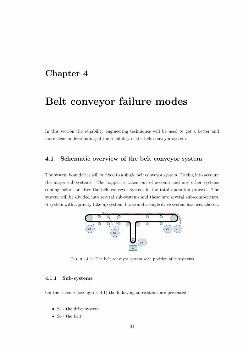
The system boundaries will be fixed to a single belt conveyor system. Taking into account
the major sub-systems. The hopper is taken out of account and any other systems
coming before or after the belt conveyor system in the total operation process. The
system will be divided into several sub-systems and these into several sub-components.
A system with a gravity take-up system, brake and a single drive system has been chosen.
Figure 4.1: The belt conveyor system with position of subsystems
4.1.1 Sub-systems
On the scheme (see figure: 4.1) the following subsystems are presented:
• S1 - the drive system
• S2 - the belt
31
32
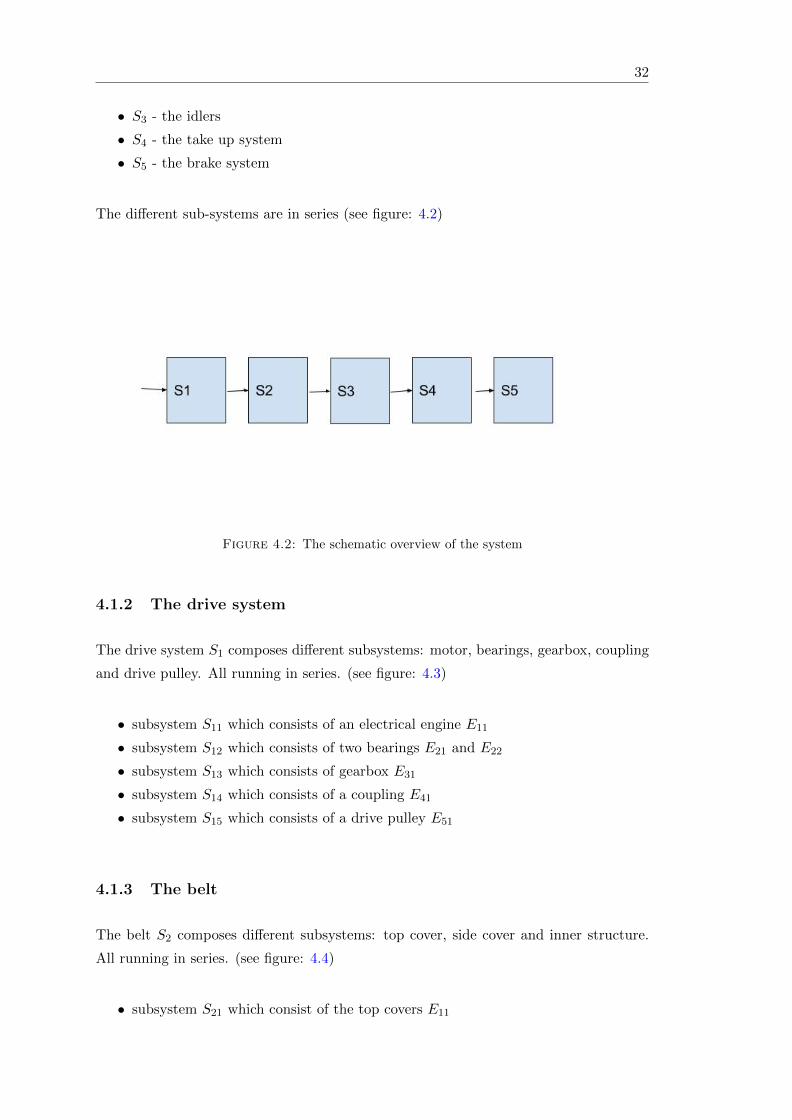
• S3 - the idlers
• S4 - the take up system
• S5 - the brake system
The different sub-systems are in series (see figure: 4.2)
Figure 4.2: The schematic overview of the system
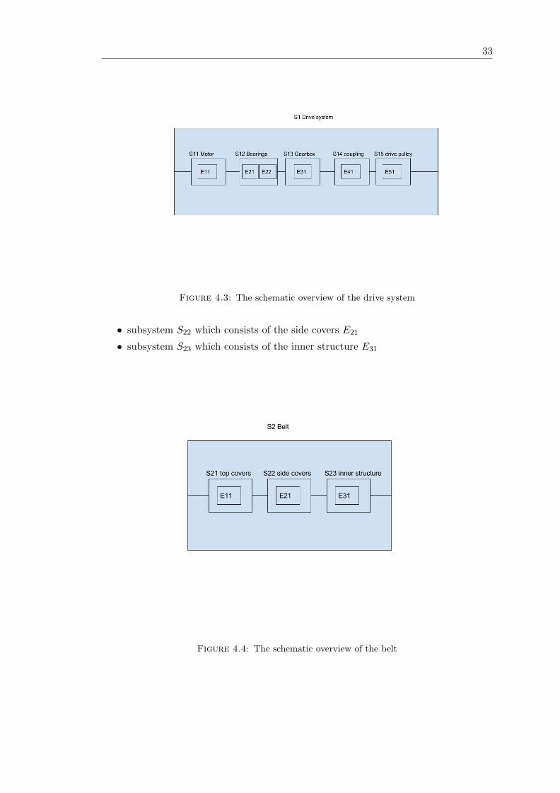
4.1.2 The drive system
The drive system S1 composes different subsystems: motor, bearings, gearbox, coupling
and drive pulley. All running in series. (see figure: 4.3)
• subsystem S11 which consists of an electrical engine E11
• subsystem S12 which consists of two bearings E21 and E22
• subsystem S13 which consists of gearbox E31
• subsystem S14 which consists of a coupling E41
• subsystem S15 which consists of a drive pulley E51
4.1.3 The belt
The belt S2 composes different subsystems: top cover, side cover and inner structure.
All running in series. (see figure: 4.4)
• subsystem S21 which consist of the top covers E11
33
Figure 4.3: The schematic overview of the drive system
• subsystem S22 which consists of the side covers E21
• subsystem S23 which consists of the inner structure E31
Figure 4.4: The schematic overview of the belt
34
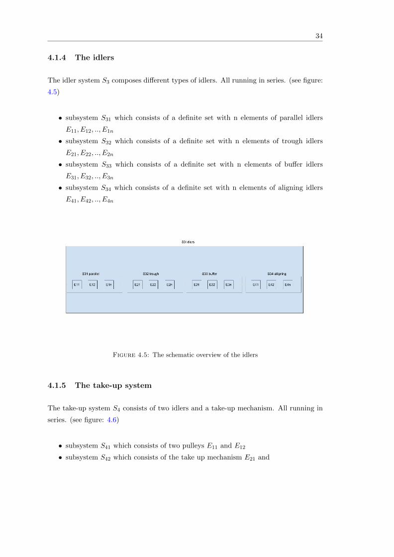
4.1.4 The idlers
The idler system S3 composes different types of idlers. All running in series. (see figure:
4.5)
• subsystem S31 which consists of a definite set with n elements of parallel idlers
E11, E12, .., E1n
• subsystem S32 which consists of a definite set with n elements of trough idlers
E21, E22, .., E2n
• subsystem S33 which consists of a definite set with n elements of buffer idlers
E31, E32, .., E3n
• subsystem S34 which consists of a definite set with n elements of aligning idlers
E41, E42, .., E4n
Figure 4.5: The schematic overview of the idlers
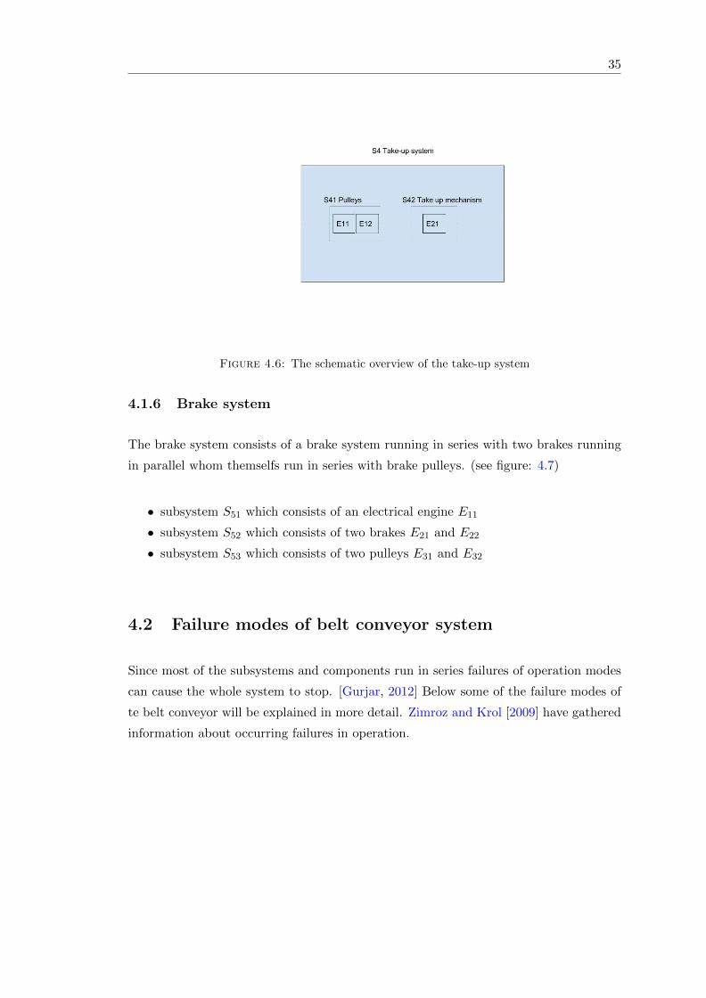
4.1.5 The take-up system
The take-up system S4 consists of two idlers and a take-up mechanism. All running in
series. (see figure: 4.6)
• subsystem S41 which consists of two pulleys E11 and E12
• subsystem S42 which consists of the take up mechanism E21 and
35
Figure 4.6: The schematic overview of the take-up system
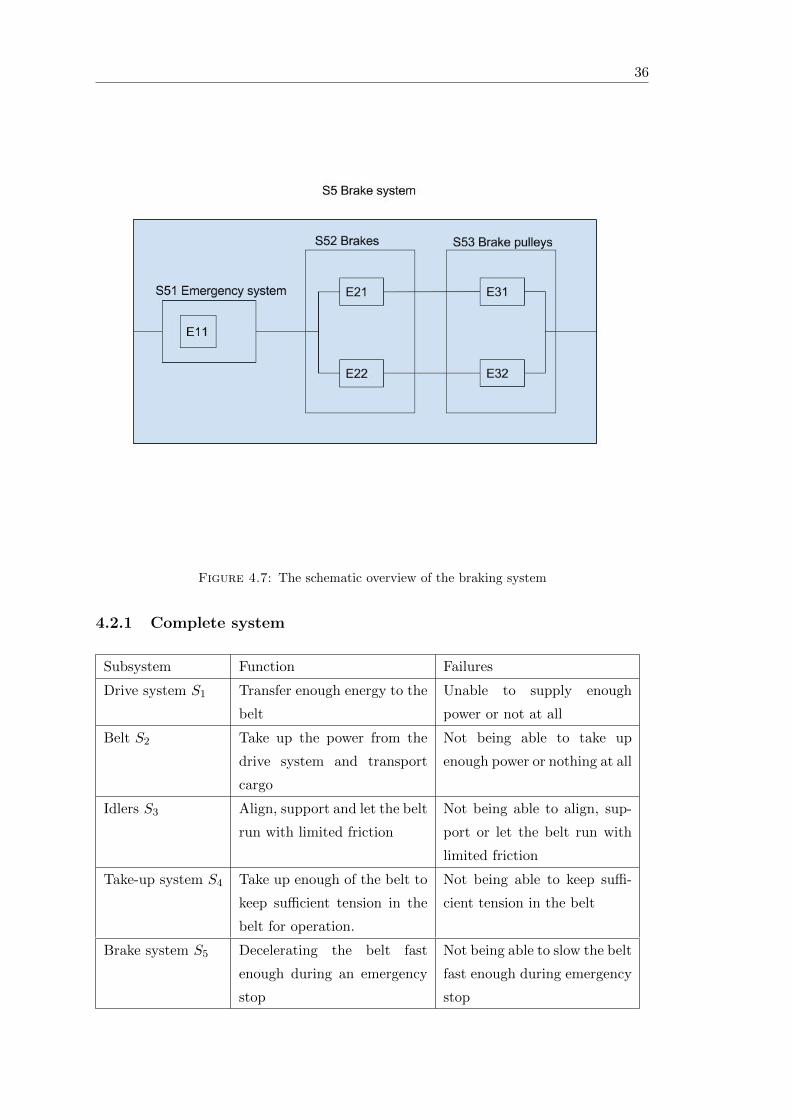
4.1.6 Brake system
The brake system consists of a brake system running in series with two brakes running
in parallel whom themselfs run in series with brake pulleys. (see figure: 4.7)
• subsystem S51 which consists of an electrical engine E11
• subsystem S52 which consists of two brakes E21 and E22
• subsystem S53 which consists of two pulleys E31 and E32
4.2 Failure modes of belt conveyor system
Since most of the subsystems and components run in series failures of operation modes
can cause the whole system to stop. [Gurjar, 2012] Below some of the failure modes of
te belt conveyor will be explained in more detail. Zimroz and Krol [2009] have gathered
information about occurring failures in operation.
36
Figure 4.7: The schematic overview of the braking system
4.2.1 Complete system
Subsystem Function Failures
Drive system S1 Transfer enough energy to the
belt
Unable to supply enough
power or not at all
Belt S2 Take up the power from the
drive system and transport
cargo
Not being able to take up
enough power or nothing at all
Idlers S3 Align, support and let the belt
run with limited friction
Not being able to align, sup-
port or let the belt run with
limited friction
Take-up system S4 Take up enough of the belt to
keep sufficient tension in the
belt for operation.
Not being able to keep suffi-
cient tension in the belt
Brake system S5 Decelerating the belt fast
enough during an emergency
stop
Not being able to slow the belt
fast enough during emergency
stop
37
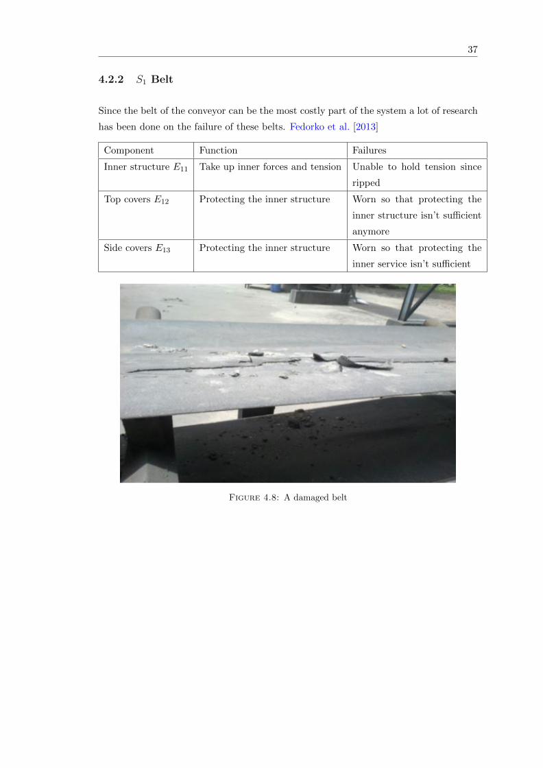
4.2.2 S1 Belt
Since the belt of the conveyor can be the most costly part of the system a lot of research
has been done on the failure of these belts. Fedorko et al. [2013]
Component Function Failures
Inner structure E11 Take up inner forces and tension Unable to hold tension since
ripped
Top covers E12 Protecting the inner structure Worn so that protecting the
inner structure isn’t sufficient
anymore
Side covers E13 Protecting the inner structure Worn so that protecting the
inner service isn’t sufficient
Figure 4.8: A damaged belt
38
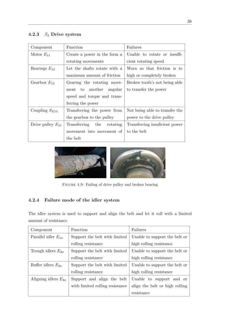
4.2.3 S2 Drive system
Component Function Failures
Motor E11 Create a power in the form a
rotating movements
Unable to rotate or insuffi-
cient rotating speed
Bearings E12 Let the shafts rotate with a
maximum amount of friction
Worn so that friction is to
high or completely broken
Gearbox E13 Gearing the rotating move-
ment to another angular
speed and torque and trans-
ferring the power
Broken tooth’s not being able
to transfer the power
Coupling SE14 Transferring the power from
the gearbox to the pulley
Not being able to transfer the
power to the drive pulley
Drive pulley E15 Transferring the rotating
movement into movement of
the belt
Transferring insuficient power
to the belt
Figure 4.9: Failing of drive pulley and broken bearing
4.2.4 Failure mode of the idler system
The idler system is used to support and align the belt and let it roll with a limited
amount of resistance.
Component Function Failures
Parallel idler E1n Support the belt with limited
rolling resistance
Unable to support the belt or
high rolling resistance
Trough idlers E2n Support the belt with limited
rolling resistance
Unable to support the belt or
high rolling resistance
Buffer idlers E3n Support the belt with limited
rolling resistance
Unable to support the belt or
high rolling resistance
Aligning idlers E4n Support and align the belt
with limited rolling resistance
Unable to support and or
align the belt or high rolling
resistance
39
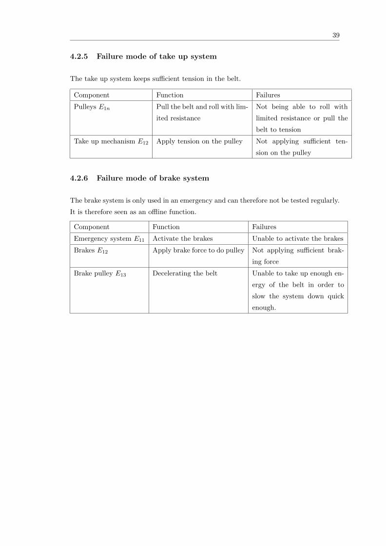
4.2.5 Failure mode of take up system
The take up system keeps sufficient tension in the belt.
Component Function Failures
Pulleys E1n Pull the belt and roll with lim-
ited resistance
Not being able to roll with
limited resistance or pull the
belt to tension
Take up mechanism E12 Apply tension on the pulley Not applying sufficient ten-
sion on the pulley
4.2.6 Failure mode of brake system
The brake system is only used in an emergency and can therefore not be tested regularly.
It is therefore seen as an offline function.
Component Function Failures
Emergency system E11 Activate the brakes Unable to activate the brakes
Brakes E12 Apply brake force to do pulley Not applying sufficient brak-
ing force
Brake pulley E13 Decelerating the belt Unable to take up enough en-
ergy of the belt in order to
slow the system down quick
enough.


Chapter 5
Operation modes
Operation processes of more complex technical systems tend to be very complex, there-
fore it is difficult to make an analysis of these systems reliability and availability with
respect to their operation conditions changing in time that are often essential in this anal-
ysis. The complexity of the systems operation processes and their influence on changing
in time the systems structures and their components reliability and safety characteristics
is often very difficult to fix. Usually, the system environment and infrastructure have
either an explicit or an implicit strong influence on the system operation process. As a
rule, some of the initiating environment events and infrastructure conditions define a set
of different operation states of the technical systems in which the systems change their
reliability and safety structure and their components reliability and safety parameters.
Levitin
5.1 Process states
In order to get a better understanding of the system it can be divided up in different
operation states. For these states we use the letter z. For a system with v, v ∈ N ,
different operations this would give. z1, z2, ..., zv. The system operations processes are
also defined by: Z(t), t ∈ 0,+∞.
5.2 Belt conveyor operation states
The following 6 operation states are defined for the belt conveyor:
• Operation state z1 - Steady state running
41
42
• Operation state z2 - Normal operational start
• Operation state z3 - Aborted start
• Operation state z4 - Normal operational stop
• Operation state z5 - Emergency stop
• Operation state z6 - In rest
Lodewijks [2014]
5.3 Time distribution operational processes
Lets assume an operational site where the operation is running during the day but is
being switched of during the night. The belt conveyor system will then be switched
on at the beginning of operations. A normal operational start z2. After the normal
operational start the system will run in steady state z1 during the normal operations.
When the operations are finished the system will be put in operation state z4, a normal
operational stop until it’s fully in rest z6.
In the case something is wrong during the start then the start will be aborted. The
system is going from z6 to z2 to z3 back to z6 again.
In the case an emergency stop needs to take place operation z5 is used.
During almost all of the time operational state z1 or z6 will be in use. Either having
the system running in steady state or in rest. In between these states in most cases z2
and z4 are in use. Only in rare occasions z3 and z5 are used.
Normal operation z6 → z2 → z1 → z4 → z6
States There were four reliability different states distinguished: (z=3)
• a reliability state 3 the system operation is fully effective
• a reliability state 2 the system operation is less effective because of ageing
• a reliability state 1 the system operation is less effective because of ageing and
more dangerous for the environment
• a reliability state 0 the system is destroyed
To satisfy the assumption on ageing, it is assumed that transitions are possible between
the components reliability states only from better to worse. Moreover, it is assumed
that the system and its components critical reliability state is r = 2.
43
Since at state 1 the system will be more dangerous for the operators and therefore
unwanted. Yingkui and Jing [2012]
5.3.1 Steady state running z1
During steady state running the system is in normal operation running at a constant
speed transporting bulk. During this type of operation the following subsystem are used
in series:
• S1 the drive system, giving the belt a steady speed
• S2 the belt running with bulk
• S3 the idlers supporting and aligning the belt
• S4 the take-up system keeping the tension in the belt sufficient
5.3.2 Normal operational start z2
During a normal operational start the system is accelerated until it reaches its desired
speed. During this type of operation the following subsystem are used in series:
• S1 the drive system, accelerating the belt
• S2 the belt running with bulk
• S3 the idlers supporting and aligning the belt
• S4 the take-up system keeping the tension in the belt sufficient
5.3.3 Normal operational stop z4
During an aborted start the accelerating is aborted to slow the system down again.
During a normal operational stop the drive unit is shut off and the system gradually
comes to a stop due to friction. The following subsystems are used in series:
• S1 the drive system is shut off
• S2 the belt running with bulk
• S3 the idlers supporting and aligning the belt
• S4 the take-up system keeping the tension in the belt sufficient
44
5.3.4 Emergency stop z5 and Aborted start z3
During an emergency stop the brakes are activated in order to quickly stop down the
system. The following subsystems are used in series:
• S2 the belt running with bulk
• S3 the idlers supporting and aligning the belt
• S4 the take-up system keeping the tension in the belt sufficient
• S5 the brake system decelerating the belt
5.3.5 System at rest z6
When the system is at rest the belt has no rotating speed. The following subsystems
are used in series:
• S2 the belt idling
• S3 the idlers supporting the belt
• S4 the take-up system keeping the tension in the belt sufficient
5.4 Fuzzy logic with Bayesian
To show the working principle of the Bayesian interference described in section 2.13
combined with the use of fuzzy logic, described in section 2.14 an example on the con-
veyor belt system is used. This shows that the method is able to make decisions based
on the monitored information.
As an example the starting z2, described in section 5.3.2 in operation of a belt conveyor
is considered. The values are fictive and the example is simplified by only considering
two causes and dividing them into two fuzzy ranges each. The Drive system S1 will
be studied during the starting operation. Two states for the functioning of the start-
ing operation will be made: tS meaning the starting time for the the conveyor belt is
sufficiently fast enough and tL meaning the starting time for the conveyor belt during
the starting operation is to long. The starting time of the conveyor belt depends on the
abrasion of the friction profile of the pulley (f) and on the delivered power by the motor
(p). The abrasion of the friction profile can be considered as low fl or as high fh. The
power delivered by the motor can be considered as normal pn or as low pl.
45
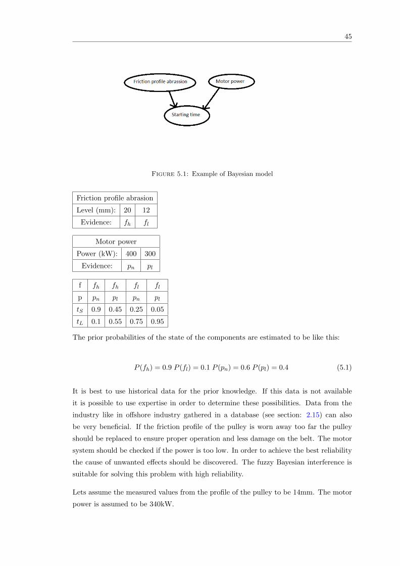
Figure 5.1: Example of Bayesian model
Friction profile abrasion
Level (mm): 20 12
Evidence: fh fl
Motor power
Power (kW): 400 300
Evidence: pn pl
f fh fh fl fl
p pn pl pn pl
tS 0.9 0.45 0.25 0.05
tL 0.1 0.55 0.75 0.95
The prior probabilities of the state of the components are estimated to be like this:
P (fh) = 0.9 P (fl) = 0.1 P (pn) = 0.6 P (pl) = 0.4 (5.1)
It is best to use historical data for the prior knowledge. If this data is not available
it is possible to use expertise in order to determine these possibilities. Data from the
industry like in offshore industry gathered in a database (see section: 2.15) can also
be very beneficial. If the friction profile of the pulley is worn away too far the pulley
should be replaced to ensure proper operation and less damage on the belt. The motor
system should be checked if the power is too low. In order to achieve the best reliability
the cause of unwanted effects should be discovered. The fuzzy Bayesian interference is
suitable for solving this problem with high reliability.
Lets assume the measured values from the profile of the pulley to be 14mm. The motor
power is assumed to be 340kW.
46
Using the fuzzy logic (see section: 2.14) to better quantify these values. The assumed
measured values are in between the two values to be considered a high or a low value.
By using a equally weighted distribution, the fuzzy values can be calculated as.
g(fh) = 0.25 g(fl) = 0.75 g(pn) = 0.4 g(pl) = 0.6 (5.2)
The updated likelihood probability P ∗ is calculated by multiplying the value of the
fuzzy membership gei(x) with the probability of that hypothesis given that event ei.
The likelihood probability is updated like:
P ∗(H|ei) = gei(x) ∗ P (H|ei) (5.3)
This way the likelihood probabilities can be updated to:
P ∗(tS |fh, pn) = g(fh) ∗ g(pn) ∗ P (tS |fh, pn) = 0.09 (5.4)
We then also find:
P ∗(tL|fh, pn) = 0.25 ∗ 0.4 ∗ 0.9 = 0.01 (5.5)
P ∗(tL|fh, pn) Means with the observation of the friction surface and the motor power
the likelihood of having a long start up due to a high friction profile and normal motor
power.
P ∗(tL|fl, pn) = 0.75 ∗ 0.4 ∗ 0.75 = 0.225 (5.6)
P ∗(tL|fl, pn) Means with the observation of the friction surface and the motor power
the likelihood of having a long start up due to a low friction profile and normal motor
power.
P ∗(tL|fh, pl) = 0.25 ∗ 0.6 ∗ 0.55 = 0.0825 (5.7)
P ∗(tL|fh, pl) Means with the observation of the friction surface and the motor power the
likelihood of having a long start up due to a high friction profile and low motor power.
P ∗(tL|fl, pl) = 0.75 ∗ 0.6 ∗ 0.95 = 0.4275 (5.8)
47
P ∗(tL|fl, pl) Means with the observation of the friction surface and the motor power the
likelihood of having a long start up due to a low friction profile and low motor power.
With the updated likelihood probabilities the posterior probabilities of f and p can be
calculated.
P (fh, pn|tL) =P ∗(tL|fh, pn) ∗ P (fh) ∗ P (pn)
P ∗(tL)= 0.082 (5.9)
P (fh, pn|tL) Means the chance of the long starting time being caused by high friction
and normal motor power.
P (fl, pn|tL) =P ∗(tL|fl, pn) ∗ P (fl) ∗ P (pn)
P ∗(tL)= 0.206 (5.10)
P (fl, pn|tL) Means the chance of the long starting time being caused by low friction and
normal motor power.
P (fh, pl|tL) =P ∗(tL|fh, pl) ∗ P (fh) ∗ P (pl)
P ∗(tL)= 0.452 (5.11)
P (fh, pl|tL) Means the chance of the long starting time being caused by high friction
and low motor power.
P (fl, pl|tL) =P ∗(tL|fl, pl) ∗ P (fl) ∗ P (pl)
P ∗(tL)= 0.260 (5.12)
P (fl, pl|tL) Means the chance of the long starting time being caused by low friction and
low motor power.
Where P ∗(tL) with i and j being the different evidences of events f and p. P ∗(tL) being
the updated marginal probability of long braking time:
P ∗(tL) =∑i,j
P ∗(tL|fi, pj) ∗ P (fi) ∗ P (pj) = 0.0054 + 0.0135 + 0.0297 + 0.0171 = 0.0657
(5.13)
The outcome of P ∗(tL|fl, pl) = 0.4275 suggests that starting time should be expected
long because of the wear of the friction pad of the idler and the low power of the motor.
The long starting time however is mainly due to the lack of motor power as can be seen by
P (fL|fh, pl) = 0.452. This one has the highest value of the four posterior probabilities.
Meaning that the main cause for the effect of a long starting time is the motor power.
This allows the system to tell that maintenance should be done on the motor.

48
As can be seen by combining the fuzzy logic with Bayesian belief network the causes of
effects can be determined in a very efficient way. This information can be used in order
to increase the overall reliability by making the right decisions in the processes.
Chapter 6
Automated reliability
optimization
A major goal in industry is the optimization of the reliability of operation systems. In
order to be safer, more reliable and more cost effective. In a lot of industries a lot of
progress has been made on this part. As is seen in the preceding chapters a belt conveyor
system is a complex system with a whole lot of subsystems and components running in
series. The most easy way to improve the overall reliability of the operation is in the form
of complete redundancy. By putting a second conveyor belt system next to the system
in order to use as a backup in the case the first one fails. Since cost is the major concern
this is certainly not always the best option. Other sectors have used reliability centered
maintenance approaches combined with automated monitoring and decision making in
order to do predictive maintenance. This technique makes the system a more smarter
system and increases reliability. At this moment in time the advanced technology of
reliability centered maintenance in industrial sectors like offshore engineering Mousavi
et al. [2013], aircraft and power-plant industries is widely implemented. In Conveyor
belt systems this is not yet the case. Currently little or no predictive maintenance is
done in conveyor belt systems. Lodewijks and Ottjes [2004]
For improving the overall reliability of belt conveyor systems the design and the main-
tenance strategy can be shifted more towards the predictive maintenance. There are
four type of maintenance strategies: Lodewijks and Ottjes [2004] random maintenance,
corrective maintenance, preventive maintenance and predictive maintenance. The use of
predictive maintenance is the most advanced. The system will be designed to monitor
the different components of the belt conveyor system and the degradation of parts is
49
50
predicted. At this way maintenance can be scheduled to improve the overall reliabil-
ity of the system. This condition based strategy allows for intelligent and automated
maintenance.
The eventual goal is to have a system with automated monitoring of the belt conveyor
components, coupled with automated decision making systems. Lodewijks [2014]
In the following section some of the modern systems for automated monitoring of differ-
ent components of the system will be explained. Later on new techniques for automatic
decision making will be explained.
6.1 Conveyor belt system monitoring
In order to get insight about the current state of the system monitoring is very important.
This can be automated to be a lot more effective, cheaper and faster.
6.1.1 Automated belt conveyor monitoring
The traditional belt conveyor monitoring and the maintenance focus on the response
of failure or abnormality of single components. With this working method detection of
problems is very late in the process not really enhancing the overall reliability of the
system. An automated belt conveyor monitoring system could detect small changes and
fluctuation in the system. By processing and analysing these subtle changes a mechanical
or electrical problem starting to develop can be derived. This allows for prediction of
possible following system failures. When the monitoring and decision making is extended
to a system level instead of separate component or sub-system level the decisions can
be made better in order to improve and optimize overall system reliability.
There have been advances in the development of systems that could be used for conveyor
belt monitoring. There are various techniques available to measure different type of
components occurrences. Some sensors measure directly, other indirectly.
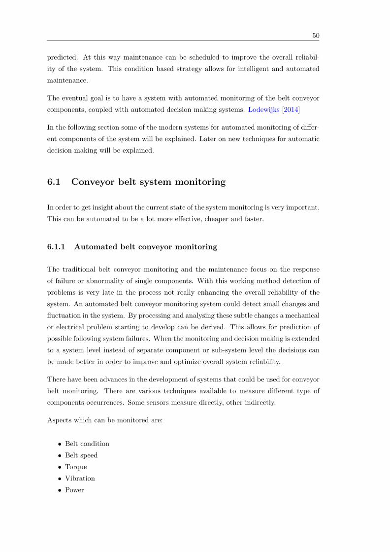
Aspects which can be monitored are:
• Belt condition
• Belt speed
• Torque
• Vibration
• Power
51
• Belt alignment
• Temperature
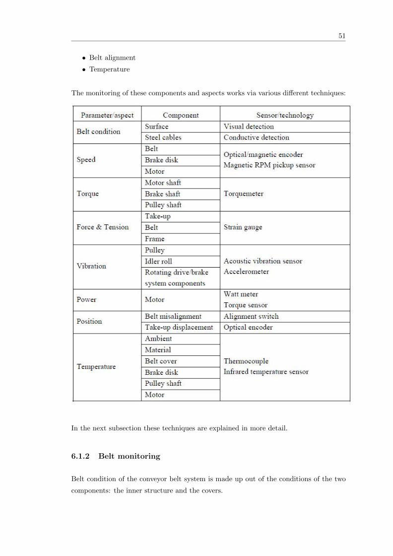
The monitoring of these components and aspects works via various different techniques:
In the next subsection these techniques are explained in more detail.
6.1.2 Belt monitoring
Belt condition of the conveyor belt system is made up out of the conditions of the two
components: the inner structure and the covers.
52
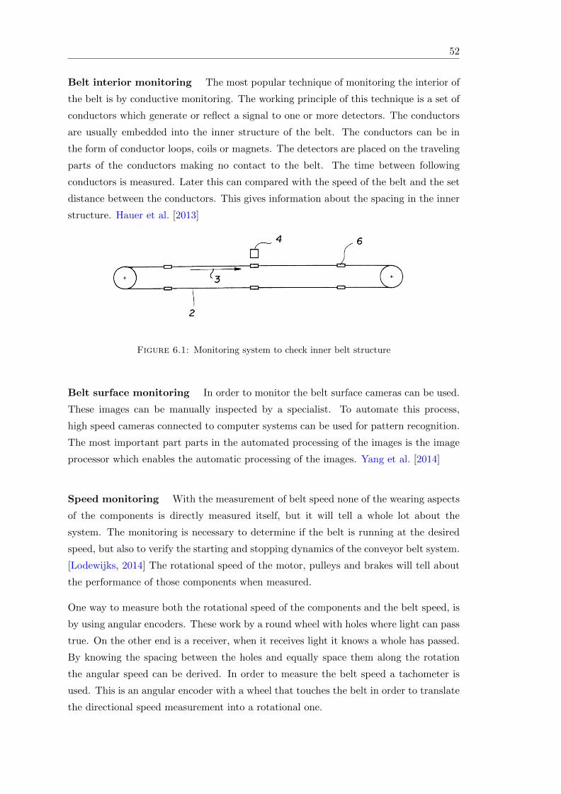
Belt interior monitoring The most popular technique of monitoring the interior of
the belt is by conductive monitoring. The working principle of this technique is a set of
conductors which generate or reflect a signal to one or more detectors. The conductors
are usually embedded into the inner structure of the belt. The conductors can be in
the form of conductor loops, coils or magnets. The detectors are placed on the traveling
parts of the conductors making no contact to the belt. The time between following
conductors is measured. Later this can compared with the speed of the belt and the set
distance between the conductors. This gives information about the spacing in the inner
structure. Hauer et al. [2013]
Figure 6.1: Monitoring system to check inner belt structure
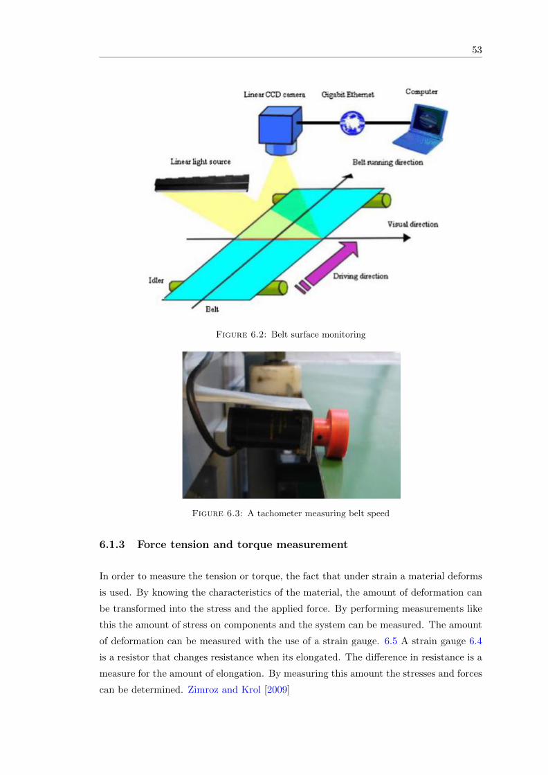
Belt surface monitoring In order to monitor the belt surface cameras can be used.
These images can be manually inspected by a specialist. To automate this process,
high speed cameras connected to computer systems can be used for pattern recognition.
The most important part parts in the automated processing of the images is the image
processor which enables the automatic processing of the images. Yang et al. [2014]
Speed monitoring With the measurement of belt speed none of the wearing aspects
of the components is directly measured itself, but it will tell a whole lot about the
system. The monitoring is necessary to determine if the belt is running at the desired
speed, but also to verify the starting and stopping dynamics of the conveyor belt system.
[Lodewijks, 2014] The rotational speed of the motor, pulleys and brakes will tell about
the performance of those components when measured.
One way to measure both the rotational speed of the components and the belt speed, is
by using angular encoders. These work by a round wheel with holes where light can pass
true. On the other end is a receiver, when it receives light it knows a whole has passed.
By knowing the spacing between the holes and equally space them along the rotation
the angular speed can be derived. In order to measure the belt speed a tachometer is
used. This is an angular encoder with a wheel that touches the belt in order to translate
the directional speed measurement into a rotational one.
53
Figure 6.2: Belt surface monitoring
Figure 6.3: A tachometer measuring belt speed
6.1.3 Force tension and torque measurement
In order to measure the tension or torque, the fact that under strain a material deforms
is used. By knowing the characteristics of the material, the amount of deformation can
be transformed into the stress and the applied force. By performing measurements like
this the amount of stress on components and the system can be measured. The amount
of deformation can be measured with the use of a strain gauge. 6.5 A strain gauge 6.4
is a resistor that changes resistance when its elongated. The difference in resistance is a
measure for the amount of elongation. By measuring this amount the stresses and forces
can be determined. Zimroz and Krol [2009]
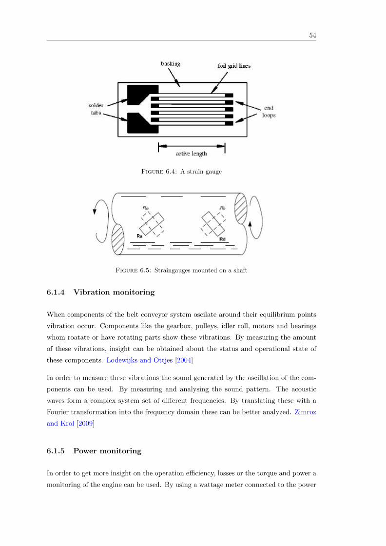
54
Figure 6.4: A strain gauge
Figure 6.5: Straingauges mounted on a shaft
6.1.4 Vibration monitoring
When components of the belt conveyor system oscilate around their equilibrium points
vibration occur. Components like the gearbox, pulleys, idler roll, motors and bearings
whom roatate or have rotating parts show these vibrations. By measuring the amount
of these vibrations, insight can be obtained about the status and operational state of
these components. Lodewijks and Ottjes [2004]
In order to measure these vibrations the sound generated by the oscillation of the com-
ponents can be used. By measuring and analysing the sound pattern. The acoustic
waves form a complex system set of different frequencies. By translating these with a
Fourier transformation into the frequency domain these can be better analyzed. Zimroz
and Krol [2009]
6.1.5 Power monitoring
In order to get more insight on the operation efficiency, losses or the torque and power a
monitoring of the engine can be used. By using a wattage meter connected to the power
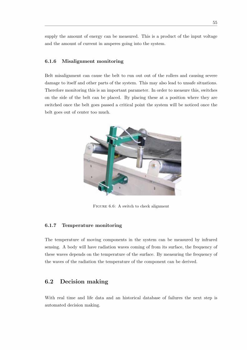
55
supply the amount of energy can be measured. This is a product of the input voltage
and the amount of current in amperes going into the system.
6.1.6 Misalignment monitoring
Belt misalignment can cause the belt to run out out of the rollers and causing severe
damage to itself and other parts of the system. This may also lead to unsafe situations.
Therefore monitoring this is an important parameter. In order to measure this, switches
on the side of the belt can be placed. By placing these at a position where they are
switched once the belt goes passed a critical point the system will be noticed once the
belt goes out of center too much.
Figure 6.6: A switch to check alignment
6.1.7 Temperature monitoring
The temperature of moving components in the system can be measured by infrared
sensing. A body will have radiation waves coming of from its surface, the frequency of
these waves depends on the temperature of the surface. By measuring the frequency of
the waves of the radiation the temperature of the component can be derived.
6.2 Decision making
With real time and life data and an historical database of failures the next step is
automated decision making.
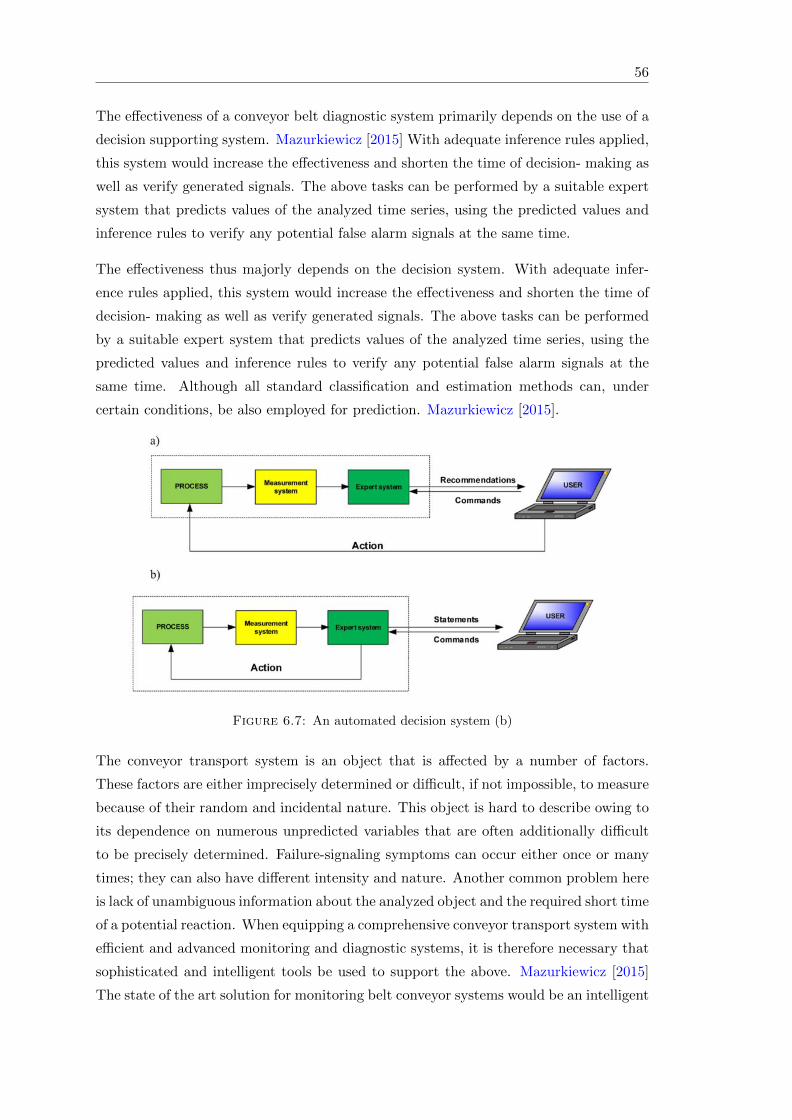
56
The effectiveness of a conveyor belt diagnostic system primarily depends on the use of a
decision supporting system. Mazurkiewicz [2015] With adequate inference rules applied,
this system would increase the effectiveness and shorten the time of decision- making as
well as verify generated signals. The above tasks can be performed by a suitable expert
system that predicts values of the analyzed time series, using the predicted values and
inference rules to verify any potential false alarm signals at the same time.
The effectiveness thus majorly depends on the decision system. With adequate infer-
ence rules applied, this system would increase the effectiveness and shorten the time of
decision- making as well as verify generated signals. The above tasks can be performed
by a suitable expert system that predicts values of the analyzed time series, using the
predicted values and inference rules to verify any potential false alarm signals at the
same time. Although all standard classification and estimation methods can, under
certain conditions, be also employed for prediction. Mazurkiewicz [2015].
Figure 6.7: An automated decision system (b)
The conveyor transport system is an object that is affected by a number of factors.
These factors are either imprecisely determined or difficult, if not impossible, to measure
because of their random and incidental nature. This object is hard to describe owing to
its dependence on numerous unpredicted variables that are often additionally difficult
to be precisely determined. Failure-signaling symptoms can occur either once or many
times; they can also have different intensity and nature. Another common problem here
is lack of unambiguous information about the analyzed object and the required short time
of a potential reaction. When equipping a comprehensive conveyor transport system with
efficient and advanced monitoring and diagnostic systems, it is therefore necessary that
sophisticated and intelligent tools be used to support the above. Mazurkiewicz [2015]
The state of the art solution for monitoring belt conveyor systems would be an intelligent

57
system that integrates the individual measurements of the system and integrates them
into one overall system, enabling decisions for maintenance and improvement to be
made at system level. This intelligent system would overcome the inability of humans
to automatically acquire and interpret data and information from the belt conveyor
system. In order to achieve these functions in a way without or less human efforts,
different kind of artificial intelligence, which have been widely applied in other sectors
can be employed. Pang and Lodewijks [2006]
6.2.1 Artificial intelligence
Mostly artificial intelligence is mostly described as non-algorithmic reasoning and auto-
matic decision making and problem solving.
• Intelligence is the calculative and deductive abilities, which are based on acquired
data and information;
• Intelligence is the probabilistic abilities to reason with uncertainty and fuzzy logic,
which are considerably contained in acquired information;
• Intelligence is the inference architecture of the human brain, which can be repre-
sented as neural network or belief network for reasoning in complexity;
• Intelligence is the intuition of human beings in making decisions based on stored
and reusable knowledge and experience;
• Intelligence is the structure of human relationships, which is organized both locally
and globally to form the integration of individual communities;
6.2.2 Assessment for intelligent monitoring system
In order to see whether artificial intelligence would be a feasible solution for the belt
conveyor system certain assessment tests have been developed. Studies show that it’s
feasible to use artificial intelligence for conveyor belt monitoring and decision making
[Pang and Lodewijks, 2006]
6.3 Reliability optimization
By implementing reliability centered maintenance in combination with automated con-
veyor belt monitoring and the automated decision making systems all ready being used
in other sectors, predictive maintenance can be performed. This will allow for scheduled
and efficient maintenance and operation. Increasing the overall reliability and saving
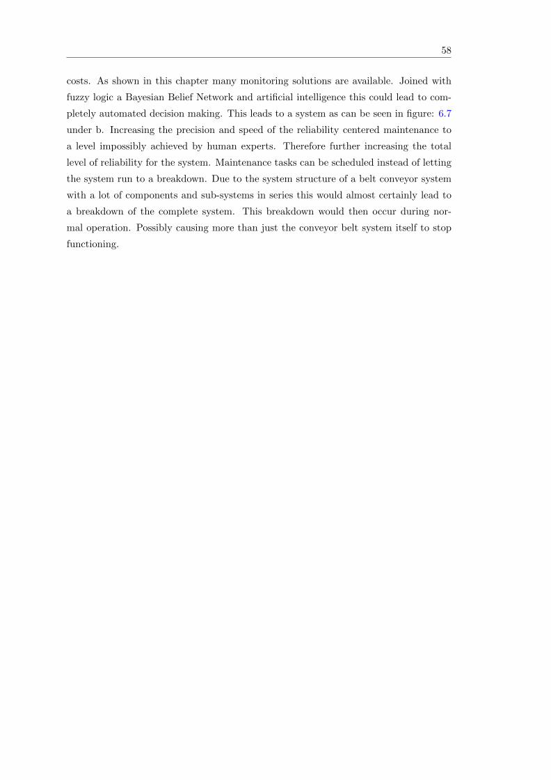
58
costs. As shown in this chapter many monitoring solutions are available. Joined with
fuzzy logic a Bayesian Belief Network and artificial intelligence this could lead to com-
pletely automated decision making. This leads to a system as can be seen in figure: 6.7
under b. Increasing the precision and speed of the reliability centered maintenance to
a level impossibly achieved by human experts. Therefore further increasing the total
level of reliability for the system. Maintenance tasks can be scheduled instead of letting
the system run to a breakdown. Due to the system structure of a belt conveyor system
with a lot of components and sub-systems in series this would almost certainly lead to
a breakdown of the complete system. This breakdown would then occur during nor-
mal operation. Possibly causing more than just the conveyor belt system itself to stop
functioning.
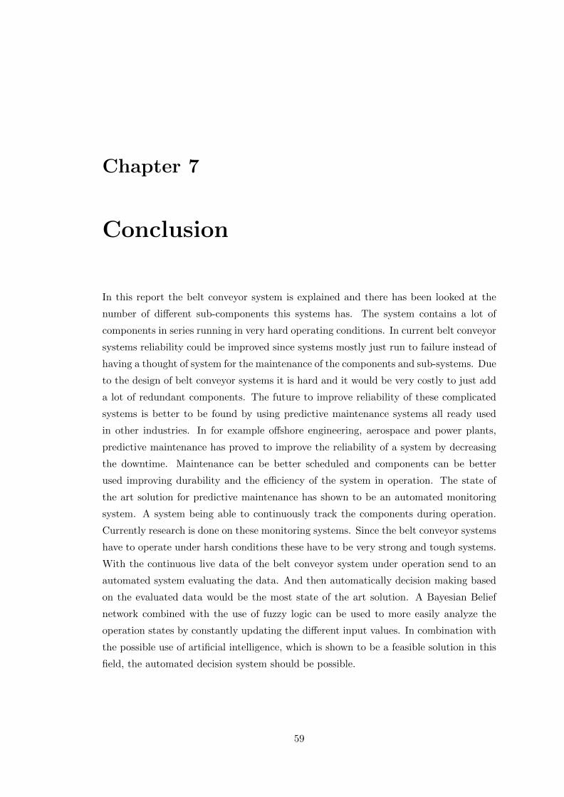
Chapter 7
Conclusion
In this report the belt conveyor system is explained and there has been looked at the
number of different sub-components this systems has. The system contains a lot of
components in series running in very hard operating conditions. In current belt conveyor
systems reliability could be improved since systems mostly just run to failure instead of
having a thought of system for the maintenance of the components and sub-systems. Due
to the design of belt conveyor systems it is hard and it would be very costly to just add
a lot of redundant components. The future to improve reliability of these complicated
systems is better to be found by using predictive maintenance systems all ready used
in other industries. In for example offshore engineering, aerospace and power plants,
predictive maintenance has proved to improve the reliability of a system by decreasing
the downtime. Maintenance can be better scheduled and components can be better
used improving durability and the efficiency of the system in operation. The state of
the art solution for predictive maintenance has shown to be an automated monitoring
system. A system being able to continuously track the components during operation.
Currently research is done on these monitoring systems. Since the belt conveyor systems
have to operate under harsh conditions these have to be very strong and tough systems.
With the continuous live data of the belt conveyor system under operation send to an
automated system evaluating the data. And then automatically decision making based
on the evaluated data would be the most state of the art solution. A Bayesian Belief
network combined with the use of fuzzy logic can be used to more easily analyze the
operation states by constantly updating the different input values. In combination with
the possible use of artificial intelligence, which is shown to be a feasible solution in this
field, the automated decision system should be possible.
59
60
7.1 Recommendations
In order make the automated predictive maintenance systems a reality. Especially in
the hard operations of belt conveyor systems more research and development has to be
done on the following: The available monitoring techniques should be further improved.
Artificial intelligence algorithms should be specifically developed for the belt conveyor
systems. Further research has to be done on how to properly interpret all the acquired
data. The eventual effects look promising as all ready shown in other industries. Allow-
ing to further improve the overall reliability of the belt conveyor systems.
Bibliography
M. a. Alspaugh. Latest Developments in Belt Conveyor Technology. MIN-
Expo 2004, page 11, 2004. URL http://www.overlandconveyor.com/pdf/
LatestDevelopmentsinBeltConveyorTechnology.pdf.
A. M. Bazzi, A. Dominguez-Garcia, and P. T. Krein. Markov reliability modeling for
induction motor drives under field-oriented control. IEEE Transactions on Power
Electronics, 27(2):534–546, 2012. ISSN 08858993. doi: 10.1109/TPEL.2011.2168543.
B. Dhillon. Mining Equipment Reliability, volume 53. 1989. ISBN 9788578110796. doi:
10.1017/CBO9781107415324.004.
G. Fedorko, V. Molnar, J. Zivcak, M. Dovica, and N. Husakova. Failure analysis of textile
rubber conveyor belt damaged by dynamic wear. Engineering Failure Analysis, 28:
103–114, Mar. 2013. ISSN 13506307. doi: 10.1016/j.engfailanal.2012.10.014. URL
http://www.sciencedirect.com/science/article/pii/S1350630712002221.
R. S. Gurjar. Failure analysis of belt conveyor system. International Journal of En-
gineering and Social Science, 2(10):11–23, 2012. ISSN 2249- 9482. URL http:
//gjmr.org/IJESS/vol2issue10/2.pdf.
I. B. Hauer, F. De, H. W. Hiiffken, C. K. Branneby, S. Feichtenhofer, G. At, M. Bucheb-
ner, G. At, B. Pohn, and G. At. ( 12 ) United States Patent U S . Patent. 2(12),
2013.
Y.-f. HOU and Q.-r. MENG. Dynamic characteristics of conveyor belts. Journal of China
University of Mining and Technology, 18(4):629–633, Dec. 2008. ISSN 10061266. doi:
10.1016/S1006-1266(08)60307-7. URL http://www.sciencedirect.com/science/
article/pii/S1006126608603077.
H. Langseth and L. Portinale. Bayesian networks in reliability. Reliability Engineer-
ing & System Safety, 92(1):92–108, Jan. 2007. ISSN 09518320. doi: 10.1016/
j.ress.2005.11.037. URL http://www.sciencedirect.com/science/article/pii/
S0951832005001985.
61
Bibliography 62
G. Levitin. Springer Series in Reliability Engineering. ISBN 9781849961141.
Z. Li, H. Liao, and D. W. Coit. A two-stage approach for multi-objective decision
making with applications to system reliability optimization. Reliability Engineer-
ing & System Safety, 94(10):1585–1592, Oct. 2009. ISSN 09518320. doi: 10.1016/
j.ress.2009.02.022. URL http://www.sciencedirect.com/science/article/pii/
S0951832009000763.
G. Lodewijks. Conveyor Belt Systems technology, 2014.
G. Lodewijks and J. a. Ottjes. Reliability of Large Scale Conveyor Systems. Proceedings
of the Industrial Simulation Conference, 2004(June):324–329, 2004.
D. Mazurkiewicz. Analysis of the ageing impact on the strength of the adhesive sealed
joints of conveyor belts. Journal of Materials Processing Technology, 208(1-3):477–
485, 2008. ISSN 09240136. doi: 10.1016/j.jmatprotec.2008.01.012. URL http://
linkinghub.elsevier.com/retrieve/pii/S0924013608000691.
D. Mazurkiewicz. Maintenance of belt conveyors using an expert system based on fuzzy
logic. Archives of Civil and Mechanical Engineering, 15(2):412–418, Feb. 2015. ISSN
16449665. doi: 10.1016/j.acme.2014.12.009. URL http://www.sciencedirect.com/
science/article/pii/S1644966514001654.
K. B. Misra and M. D. Ljubojevic. Optimal Reliability Design of a System: A New
Look. IEEE Transactions on Reliability, R-22(5):255–258, 1973. ISSN 0018-9529.
doi: 10.1109/TR.1973.5215673.
M. E. Mousavi, P. Gardoni, and M. Maadooliat. Progressive reliability method and
its application to offshore mooring systems. Engineering Structures, 56(0):2131–2138,
2013. ISSN 0141-0296. doi: http://dx.doi.org/10.1016/j.engstruct.2013.08.016. URL
http://www.sciencedirect.com/science/article/pii/S0141029613003830.
Y. Pang and G. Lodewijks. System for Intelligent Conveyor Belt Monitoring. pages
803–808, 2006.
M. Rausand. Reliability centered maintenance. Reliability Engineering & System Safety,
60(2):121–132, 1998. ISSN 09518320. doi: 10.1016/S0951-8320(98)83005-6. URL
http://www.sciencedirect.com/science/article/pii/S0951832098830056.
M. Rausand and K. Ø ien. The basic concepts of failure analysis. Reliability Engineering
& System Safety, 53:73–83, 1996. ISSN 09518320. doi: 10.1016/0951-8320(96)00010-5.
Y. Yang, C. Miao, X. Li, and X. Mei. On-line conveyor belts inspection based on
machine vision. Optik - International Journal for Light and Electron Optics, 125

Bibliography 63
(19):5803–5807, Oct. 2014. ISSN 00304026. doi: 10.1016/j.ijleo.2014.07.070. URL
http://www.sciencedirect.com/science/article/pii/S0030402614008304.
G. Yingkui and L. Jing. Multi-State System Reliability: A New and Systematic Re-
view. Procedia Engineering, 29:531–536, 2012. ISSN 18777058. doi: 10.1016/j.
proeng.2011.12.756. URL http://www.sciencedirect.com/science/article/pii/
S1877705811065933.
Zadeh. The role of fuzzy logic. 11:199–227, 1983.
L. Zhao and Y. Lin. Typical failure analysis and processing of belt conveyor. Procedia
Engineering, 26:942–946, 2011. ISSN 18777058. doi: 10.1016/j.proeng.2011.11.2260.
URL http://dx.doi.org/10.1016/j.proeng.2011.11.2260.
R. Zimroz and R. Krol. Failure analysis of belt conveyor systems for condition monitoring
purposes. Studia i Materiay, (36):255–270, 2009.


![1 SERIES Belt Conveyor System B090 - Bett Sistemi Srl€¦ · CONVEYOR BELT DEVELOPMENT CALCULATION FORMULA Conveyor belt length = 300 + {[(L-94)-(2• Conveyor belt thick. )]•2}](https://img.dokumen.tips/doc/110x75/5ad3c4047f8b9a48398b7ae4/1-series-belt-conveyor-system-b090-bett-sistemi-conveyor-belt-development-calculation.jpg)