NASA Technical Memorandum 86750

Symbolic Generation of ElasticRotor Blade Equations Using aFORTRAN Processor andNumerical Study on DynamicInflow Effects on the Stability ofHelicopter RotorsT. S. R. Reddy, Ames Research Center, Moffett Field, California

June1986

NP ANational Aeronautics andSpace Administration

Ames Research CenterMoffett Field, California 94035

https://ntrs.nasa.gov/search.jsp?R=19870015022 2020-04-09T17:57:06+00:00Z

SYMBOLS

a

AIj,A2j,A3j,GIi

b

BIj,B2j,B3j,G2i

C

Cdo

CIj,C2j,C3j,G3i

CT,CM,C L

CT,CH,Cw

Cmx,Cmy

F

f

J

KA

N1, 2

L

[wp

M

[MI,[CI,[KI

[ml,[_l

lift-curve slope, 2_/radian

row matrices, equation (16c)

number of blades

row matrices, equation (16c)

chord, m

profile drag coefficient

equivalent drag coefficient, equation (14)

row matrices, equation (16c)

harmonic perturbation coefficients of thrust pitching moment, and

rolling moment, equation (11)

rotor steady thrust, drag force and weight coefficient, equa-

tion (32)

rotor steady pitch and roll moments, equation (32)

forcing function, equation (27)

flat plate area, m2

number of points used in harmonic analysis, equation (28)

blade cross-section polar radius of gyration, m

principal mass radii of gyration, m

blade cross-section mass radius of gyration, m

number of harmonics used in the harmonic analysis

perturbed aerodynamic force in flap direction

number of coupled rotating modes

constant mass, damping and stiffness matrices, equation (27)

dynamic inflow matrices

PRECED|NG PAGE BLANK NOT FLIED

v _|NT[NTIONALLY BLANK

N

n

qo,qc,qs

R

UT,U P

vi

W,V,¢

Woj,Voj,*oJ

Xjk

Xoj,Xcj,Xsj

x

a R

8pc

Y

y*

Awj,_Vj,A,j

_k,mk

ni,_i,Si

8

oj

x

total number of blade modes used

number of the harmonic in harmonic analysis, equation (30)

vectors of collective and cyclic modes, respectively

rotor radius, m

tangential and perpendicular velocity components, m/sec

induced velocity

flap, lag and torsion deflections

steady flap, lag and torsion deflections, equation (8)

generalized coordinate of jth mode of kth blade

multiblade coordinates of Jth mode, equations (17) and (38)

blade coordinate along the radius

rotor shaft plane angle of attack, equation (32)

wake skew angle, equation (25)

precone angle, radian

Lock number

equivalent Lock number, equation (14)

perturbation flap, lag and torsion deflections, equation (8)

real and imaginary parts of the characteristic exponent

mode shapes for flap, lag and torsion

pitch angle, radian

blade torsion mode shape

steady inflow

advance ratio

inflow parameter, equations (12) and (26)

vl

U0 ,U c ,U s

a

_W '_V '_¢

( )

()'

(')*

( )k

uniform, longitudinal, and lateral inflow components

air density, kg/m 3

solidity ratio, = bc/_R

azimuthal angle, nondimensional time

blade rotational speed, radian/sec

nondimensional rotating flap, lag, and torsional frequencies

nondimensionalized quantity, equilibrium deflection

space derivative

time derivative

quantity associated with kth blade

vii

SUMMARY

The process of performing an automated aeroelastic stability analysis for an

elastlc-bladed helicopter rotor is discussed. A symbolic manipulation program,

written in FORTRAN, is used to aid in the derivation of the governing equations of

motion for the elastic-bladed rotor. The blades undergo coupled bending and tor-

sional deformations. Two-dimensional quasi-steady aerodynamics below stall are

used. Although reversed flow effects are neglected, unsteady effects, modeled as

dynamic inflow are included. Using a Lagranglan approach, the governing equations

are derived in generalized coordinates using the symbolic program. The symbolic

program generates the steady and perturbed equations and writes into subroutines to

be called by numerical routines. The symbolic program can operate both on expres-

sions and on matrices. For the case of hovering flight, the blade and dynamic

inflow equations are converted to equations in a multiblade coordinate system by

rearranging the coefficients of the equations. For the case of forward flight, the

multiblade equations are obtained through the symbolic program. The final multi-

blade equations are capable of accommodating any number of elastic blade modes. The

computer implementation of this procedure consists of three stages: (I) the sym-

bolic derivation of equations; (2) the coding of the equations into subroutines; and

(3) the numerical study after identifying mass, damping, and stiffness coefficients

for each equation. Damping results are presented in hover and in forward flight

with, and without, dynamic inflow effects for various rotor blade models, including

rigid blade lag-flap, elastic flap-lag, flap-lag-torsion, and quasi-static tor-

sion. Results from dynamic inflow effects which are obtained from a lift deficiency

function for a quasi-static inflow model in hover are also presented.

The numerical results for hovering flight indicate that dynamic inflow

increases the lead-lag regressing-mode damping for torsionally rigid blades. For

torsionally flexible blades, the dynamic inflow effect depends on the elastic cou-

pling parameter. For zero elastic coupling, dynamic inflow increases the modal

damping. For full elastic coupling, it decreases the damping. This implies that

there exists an elastic coupling parameter value for which dynamic inflow effects

are negligible. The study for forward flight indicates that for a large number of

degrees of freedom and nonlinear models, the amount of input data to the symbolic

program increases exponentially, making it inconvenient to explicitly consider the

harmonic and multlblade equations. However, a combination of symbolic and numerical

programs at the proper stage inthe derivation process makes it effective and bene-

ficial to obtain the stability results from this approach. The numerical study

indicates that dynamic inflow does change the magnitude of the predicted damping,

yet its influence on damping trends is generally small with varying advance ratio or

elastic-coupling parameter for torsionally flexible blades. In this report, Part I

describes the symbolic program concepts. Part _I presents the numerical results

obtained using this process.

INTRODUCTION

It is a general experience that derivation of governing equations of motion forcomplex structures represents a task of significant magnitude and is subject toerror whenperformed by hand. Whenconsideration is given to helicopter aeroelasticproblems in particular, even for a rigid flap-lag model, the derivation of thegoverning equations of motion and the multiblade coordinate transformation requiresmuch time and determination of accuracy by independent means. Experience withelastic hingeless rotor blade analyses indicates that for a given ordering scheme,the final equations differ in small nonlinear terms in the process of derivationdepending on the stage at which the ordering schemeis applied. Whenthe orderingschemeis consistently applied at a later stage in the derivation process, in gen-eral, this process requires more time and more lengthy independent checking.

In this situation, a symbolic manipulator allows the analyst to share thealgebra with the computer. Use of symbolic programs has been reported in severalbranches of science and engineering for over 30 years. There are manygeneralsymbolic processors available, for example, MACSYMA(ref. I), REDUCE,etc., writtenin LISP. MACSYMAhas been used in manystructural applications (ref. 2), and REDUCEhas been used in helicopter applications (ref. 3). Whenapplied to a particularproblem, the numerouscapabilities available from such general purpose programs tendto slow the program execution and puts restrictions on computer memory.

To circumvent these shortcomings, programs have been developed which are spe-cially tailored to given tasks, as for example, in celestial mechanics(refs. 4-9). These programs take advantage of the special form of the expressionsto be manipulated. They deal with the powers of the fixed numberof variablesforming the expressions and they manipulate the algebraic operations. These pro-grams were written partly in FORTRANand partly in machine language. In refer-ence 10, concepts have been presented to manipulate matrices and series (expres-sions) of general form using FORTRAN.Using these basic concepts, a program calledHESLhas been written in FORTRAN(ref. 11) and was used in deriving rigid bladehelicopter rotor equations for aeroelastic analysis.

In the present study, HESLhas been extended and used in the derivation ofelastic blade equations in generalized coordinates using a Lagrangian formulation.The equations can be derived for any given ordering scheme. These equations arecoded into FORTRANsubroutines. The statements such as the subroutine namesCOMMON,DIMENSION,etc., which are required in making these subroutines are read as dataduring the coding. The program writes two subroutines, one for nonlinear equationsto calculate the rotor trim position and the other for use with linearlzed perturba-tion equations to analyze stability. These subroutines are subsequently called bynumerical routines which identify the mass, damping, stiffness, and load terms foreach equation to form the required matrices which govern the blade behavior. Har-monic balance equations and transformed multiblade coordinate equations are obtainedfrom the symbolic program. A schematic of the entire operation is shown infigure 1(a). The figure shows three segments of the analysis process; segment I for

2

computer derivation of the equations, segment 2 for incorporating the matrix ele-ments into FORTRANsubroutines, and segment 3 for numerical study.

In this report, Part I describes the symbolic program aspects and Part IIpresents numerical results on the aeroelastic stability of an elastic rotor withdynamic inflow both in hover and in forward flight.

I: SYMBOLICPROCESSORPROGRAMPRINCIPLES

In this section, the concepts used to develop a symbolic (algebraic} manipula-tion program using FORTRANare described. The basic manipulation of multiplying twoexpressions symbolically is then explained. Using this manipulation, the algebraicoperations required in the aeroelastic stability and in response analysis of heli-copter rotors are developed and presented. The matrix operations are performed byassuming that the elements of the matrix are expressions. The remaining sectionsexplain the modeof input to the symbolic program. A sample output from the compu-ter program is given in appendix A. All the symbols used in this section are givenin table AI.

Program HESL

Reading and storing information- The basic principle (refs. 10 and 11) is to

associate numbers with the variables (blade deflections, rotations, and time deriva-

tives) that are to be manipulated. This allows numbers instead of variables to be

manipulated. The program automatically assigns a number to the variable as soon as

it reads it for the first time. Initially the program assumes that an expression or

a relation is composed of a number of individual terms. Each term within an expres-

sion or a relation consists of (I) a single numerical coefficient, and (2) a pattern

which consists of the numbers associated with each variable in the term. For exam-

ple, tension T is given by

1 2 1 ,2T = EA u' + _ v' + _ w (la)

where E is Young's modulus, A is the area of cross section, u' is the derivative

of the extensional displacement, and v' and w' are bending slopes in two planes.

The equation for T could be defined as an expression given by

T : E*A*(I.0*US + 0.5*VS*VS + 0.5*WS*WS)

(expression) = (term) + (term) + (term)

(lb)

which contains three terms. Each term has a numerical coefficient and is made up of

variables US, VS, WS, E, and A. The data for each term are read in alphanumeric

format (e.g., FIO.O, At, A4), and numbers are assigned by the program to variables

E, A, US, VS, and WS. Let I, 2, 3, 4, and 5 respectively, be the numbers assigned

to these variables. Then the first term (E A US) has a numerical coefficient of 1.O

and a pattern of 1 2 3. The second term (0.5 E A VS VS) has a numerical coefficient

of 0.5 and a pattern of 1 2 4 4; the third term has a numerical coefficient of 0.5

and a pattern of I 2 5 5. In the program, the expression T is (where brackets are

used for convenience)

T : 1.0(I)(2)(3) + 0.5(I)(2)(4)(4) + 0.5(I)(2)(5)(5) (2)

As another example, a relation given in a table which is used for subsequent substi-

tution later in the derivation process might be

e : e0 + ec cos _ + es sinTHTA : 1.0*THTO + 1.0*THTC*CSCY + 1.0*THTS*SNCY

(relation) : (term) + (term) + (term)

(3)

which shows the total pitch angle as given by collective and cyclic pitch angles

and _ is nondimensionalized time. By letting 6, 7, 8, 9, 10, 11 represent THETA,

THTO, THIC, CSCY, THTS, and SNCY, equation (3) in the program is

(6) = 1.0(7) + 1.0(8)(9) + 1.0(10)(11) (4)

The numerical coefficient and the pattern of each term are stored in a coefficient-

storage stack (or array), and in a pattern storage stack. These stacks are common

to all expressions and to all relations given for integration, differentiation,

perturbation, trigonometric relations for multiblade coordinate transformation,

etc. The definition of expressions and relations and their storing is schematically

shown in figure 1(b). A separate array (expression array) is provided to store the

number of terms of the expression, such as T, its identification number, and the

starting position in both the storage stacks. This information is required for

subsequent expression retrieval. Similarly, the relations (right-hand side of THTA,

in eq. 3) required for integration, differentiation, perturbation, etc., are read as

tables of relations and are stored in stacks. The starting position and number of

terms of the relations (THTA) for all the tables (distinguished by different table

names), table identification number and left-hand side of the relation (THTA), are

stored in a table array for retrieval. If the relations are not available in closed

form, numerical schemes are used. The elements of a matrix are assumed to be formed

by expressions. A matrix array stores the number of rows and columns of the

matrices and the position of the corresponding numerical coefficient and pattern of

the elements of the matrix in the storage stacks.

Special symbols are provided to identify a variable, symbol ' ' (blank), an

expression, symbol '%', a matrix, symbol '#', a table containing known relations,

symbol '@' For example, expression T (eq. (I)) is identified as an expression in

the program by placing the symbol % in front of the expression. Similarly, varia-

bles WS, US, VS, THTO, THTC, THTS, CSCY, and SNCY are recognized as variables by

placing a blank before them. Let the table containing relation (eq. (3)) be named

TRIG. It is identified in the program by placing '@' in front of the table name as

@TRIG.

Algebraic manipulation- The basic manipulation is the multiplication of two

expressions, say X and Y, to get expression Z. The details of X and Y are

obtained from the expression array (number of terms, starting location in common

stacks), and from the common stacks (numerical coefficient and pattern of each

term). The multiplication is then performed term by term. The product of two terms

yields a new term. The numerical coefficient of the new term is the product of the

numerical coefficients of the two terms. The pattern of the new term is the conca-

tenation of the patterns of the two terms in the product. For example, if term

E A US and term 0.5E A VS VS are multiplied, we get the new term

0.5 E A US E A VS VS, which in symbolic notation becomes

O.5(I)(2)(3)(I)(2)(4)(4)

After all the terms are multiplied, the resulting terms are stored in the

common stacks. The location of these terms in the common stacks, and the number of

terms of the expression Z, and identification number for Z are stored in the

expression array for retrieval.

The second manipulation is substituting relations, given in a table within the

computer code, into an expression. This is conceived as substituting the pattern

for the relation (such as the pattern for THTA) into an expression containing THTA

and carrying out the required multiplication, as explained above. The position of

THTA in the common stacks is obtained from the table array. It can be seen that

integration, perturbation, multiblade coordinate transformation, etc., can be easily

performed with the known relations in this way. For differentiation, the same

substitution technique is used; however, care is taken to store the dependent and

independent variables separately. It can be realized that substitution of known

relations for integration and differentiation is similar to the table look up proce-

dure used in many aerodynamic calculations.

A compacting capability is provided for the addition of similar terms within an

expression. This is done by comparing two terms within an expression for patterns,

and, if they are identical, numerical coefficients are added and the number of terms

in the expression is reduced by one.

The ordering scheme is applied in the following manner. The order of each

variable and the overall ordering scheme are read as user-supplied data. Once all

the terms in each expression are determined, the order of each variable is added on

a term-by-term basis. If the order sum for a particular term is greater than the

specified order to be retained, the term is neglected.

In order to collect all the coefficients that multiply a state variable in the

final equations, the pattern of each term is checked to see whether the number

assigned to that state variable is present. If it is present, the term is stored

separately.

To perform a multiblade transformation, the relevant trigonometric relationsare supplied as a table of relations. The multiblade functions I, cos _, sin _,etc., are read as data depending on the numberof blades. For example, these func-tions for a five-bladed rotor are I, cos _, sin _, cos 2_, and sin 2_. The multi-blade expansion of each generalized coordinate is givenas data. Then the requiredmultiplications and substitutions are performed. The terms are then checked forcos N_ and sin N_ (N = numberof blades). Terms which do not have integer multiplesof numberof blades are deleted. Harmonic balance equations are obtained by substi-tuting the trigonometric relations and by collecting all like harmonics.

Using the above concepts, the program HESLwas written in FORTRANand used togenerate the governing equations of motion of a coupled rigid fuselage and rigidrotor blade analysis (ref. 11). HESLcan perform all the algebraic manipulationsrequired in the equation derivation. It can perform these operations at an expres-sion level or matrix level. Matrix multiplication, transpose multiplication, addi-tion, subtraction, and multiplication of matrix elements with a constant or expres-sion can be done by using HESL. The matrix operations are done by assuming that theelements of the matrix are expressions. The matrix elements can be changed toexpressions. As explained above, integration, differentiation, perturbation, andmultiblade coordinate transformations are done by substituting knownrelationsprovided as data to the program. Numerical schemesare used if necessary. Itshould be noted that for the harmonic balance equations and multiblade coordinatetransformation, trigonometric relations (products of sines and cosines expressed assumsof sines and cosines) are given as a table of relations and substitution isdone. Equations can be derived for any ordering scheme.

The program has 40 subroutines excluding numerical routines, and are calledthrough a main program by reading the manipulations to be performed as commands.For example, the commandFORMEXPRESSIONis used to call the necessary subroutinesto multiply two or more expressions. The commandFORMMATRIXis used to call thesubroutines to multiply two matrices. The commandSUBSTITUTETABLEINTOEXPRESSIONwill substitute known relations into an expression, etc. The HESLcode has22 recognized commands. Table I lists each of the various commandsand theirfunctions.

The basic input to the program are the position vector, transformation rela-tions, order of each variable, and the ordering scheme. If the relations are known,the relations for integration, differentiation, perturbation, etc., are given astables of relations. The nonlinear equations are obtained by calculating strainenergy, kinetic energy, and work done in generalized coordinates, then a Lagrangianformulation is used to obtain the governing equations of motion. The equations arelinearized using the perturbation relations. Whenusing trigonometric relations,harmonic balance equations and multiblade equations are obtained. The multibladesummation rules are embeddedin the program. It should be noted that apart from thebasic relations, the data to generate a required function has to be given asinput. For example, one has to define what functions are to be multiplied to getstrain energy. For a different blade model only the basic relations that define thechange in the model need to be defined.

Data and program aspects- The main program initializes the program data, reads

the commands, and calls the appropriate subroutines. When it encounters the com-

mand, END OF DATA, execution is stopped. In order to keep the available core space

to a maximum, all the expressions which are no longer needed are erased from the

common stacks by a RESET COUNTER.

The first input line in the program deck defines the identifiers to be used for

a blank variable 'bbb', a variable 'b', an expression '%', a table '@', and a matrix

'#' in that order.

This first input line is immediately followed by the input for the algebraic

manipulations:

12345678

bbbbb%@#

column numbers (not an input)

(b denotes a blank space)

In general the input is the command name, followed by the name of the expression

(table, matrix) and number of terms (relations, size) of the expression (table,

matrix) followed by the term (relation, term) details. These expressions are in

fixed format so as to provide consistency and to avoid confusion.

The names of variables, expressions, matrices, and tables are restricted to

four alphanumeric characters and are read in A4 format. The identifiers are read in

AI format. For example, variables WS and VS are recognized by reading them as bbbWS

and bbbVS. Expressions T and VEL are read as %bbbT and %bVEL, matrix LAFP is read

as #LAFP. Table TRIG which contains given relations is read as @TRIG. Other sym-

bols are used to separate them from this predefined set. For example, symbol '*' in

*E2DI is used for identifying an ordering scheme, and symbol "e' in ePECF is used

for identifying a group having certain variables.

The terms of an expression or relation are read as input with only one term for

each input line. The first ten columns of the line are reserved for the numerical

constant and the remaining columns are used for the variables (or expressions)

forming the term. The format is

FIO.O,14(AI,A4) (5)

For example, the term 0.5 WS WS VS VS is read as

123456789012345678901234567890 column numbers (not an input)

0.5bbbbbbbbbbWSbbbWSbbbVSbbbVS

The input and output of the program can be best explained for an example by

deriving equations for the flap motion of a rotor blade model. Appendix A gives the

complete input and output for the problem chosen. The problem definition starts

with a flap-lag transformation definition, but is subsequently reduced to a flap-

only model. This simplified model is used to clarify the program aspects rather

than clarifying the modeling aspects. It should be noted that other forms of

achieving the required objective may exist in addition to those defined here which

use the basic algebraic manipulations. Table AI shows all the symbols used in the

program.

The following explains how commands and data are read to the program. The data

can be considered as consisting of two parts. One is directly read by the read

commands (READ EXPRESSION, READ TABLE, etc.). For the second, data operations for

the manipulations, i.e., FORM EXPRESSION, FORM MATRIX, SUBSTITUTE TABLE INTO EXPRES-

SION, etc., are used. The commands can be divided into three parts: (I) Input

Commands; (b) Algebraic Manipulation Commands; and (3) Application Commands (see

table I).

General Rules

I. Commands names are entered from the first column. Only the first eight

characters of the command are important for the operation.

2. The names of variables, expressions, matrices, and tables are always asso-

ciated with their identifiers7 ' ', '%', '#', and '@', respectively (read in the

first input line).

3. Other identifiers can be used to distinguish them from variables, expres-

sions, matrices, and tables, for example, *,e,1, to be used in specifying ordering

schemes, group names for collection of coefficients.

Input commands- These commands are used to read the input data, such as details

of the terms forming the expressions, matrices, and tables of relations.

Command "READ EXPRESSION". This command is used to input an expression con-

sisting of variables only. The input sequence is:

I. Command name;

2. Expression identifier (%), expression name, and the number of terms in the

expression in format (AI,A4,12);

3. For each term, input details of the term in format (FIO.O,14(A1,A4)).

Example to input the strain energy of the blade given by

ISeb _ : _ Kp 82

where K8 is the flapping stiffness andexpression T given by

8 is the flapping angle and to read

I ,2 I w,2T = EA u' + _ v + _

8

Input Explanation

123456789012345678901234567890

READ EXPRESSION

%SEBLOI

0.5 KBT BT BT

READ EXPRESSION

% TO3

1.O E A US

0.5 E A WS

0.5 E A VS

WS

VS

(column numbers, not an input)

command name.

identifier, expression name, number of terms.

numerical coeff., variables KBT,BT forming the

term.

command name.

identifier, expression name, number of terms.

numerical coeffi., variables E,A, US.

numerical coeffi., variables E,A, WS,WS.

numerical coeffi., variables E,A, VS,VS.

Command "READ MATRIX". This command is used to input the elements of a

matrix. The term details of the matrix A are read as (A(I,J),J=I,N),I=I,M). The

terms of the matrix element can be variables or already defined expressions or a

combination of these expressions. The input sequence is:

I. Command name ;

2. Matrix identifier (#), matrix name, size of the matrix (rows by columns),

and ordering scheme if required, in the format (A1,A4,212,AI,A4);

3. Then for each element of the matrix, read the number of terms and for each

term read the term details in format (F10.O,14(AI,A4). Example: To input the flap

transformation matrix, given as

[cos0Tfl p : 0 I 0

sin 8 0 cos

where 8 is the flapping angle.

Input Explanation

12345678901234567890

1234567890

READ MATRIX

#TFLP0303

Ol

I.O COSB

O1

(column nunlbers, not an input)

command name.

matrix identifier, matrix name, number of rows,

number of columns.

number of terms in element T(1,1).

numerical coefficient, variable COSB

(COSB is cos S).

number of terms in element T(I,2).

Input (cont'd) Explanation

0.0

01

-I .0 SINB

01

0.0

01

1.0

01

0.0

01

1.0

01

0.0

01

1.0

SINB

COSB

numerical coefficient.

number of terms in element T(1,3).

numerical coefficient, variable SINB

(SINB is sin 8).

number of terms in element T(2,1).

Command "READ TABLE FOR SUBSTITUTION". This command is used for reading a

table of relations which is used in subsequent substitutions. Each table of rela-

tions is identified by a table name. HESL identifies two types of tables of rela-

tions. Type I is a substitution of relations of the type v = v + 6v, and type 2 is

a relations table which has powers (>I) and a product of the variables such as

sin 2 @ = 0.5-0.5"cos 2_. In type 2, the relations can be handled in the general

form of A£BmC n = terms, where A, B, _nd C _re variables, and £, m, and n aretheir powers. For example, sin 3 _ cos e sin 8 = terms. The input sequence is:

I. Command name;

2. Table identifier (#), table name, number of relations in the table, and

type of the table used in format (AI,A4,12). A zero value indicates type I rela-"

tions, a nonzero value indicates type 2 relations;

3. Then, for each relation, input:

(a) the number of terms on the right-hand side of the relation, the left-

hand side variables and their power in format (I2,4(A4,12));

(b) the details of the terms (of the right-hand side of the relation) in

format (F10.O,14(A1,A4)).

Example: To input two tables of relations. Table I, named SUPR contains

powers of unity of the variables in the relation. Table 2 contains powers greater

than the unity of the variables and the product of variables.

Table I (I) sin _ = 0.0; (2) cos _ = 1.0; (3) e = e + 0 cos @ + e sin0 C S

10

Table 2(I) sin 2 B = 1.0 - 1.0 cos 8 cos 8; (2) sin _ cos2 _ = 0.25 sin _ + 0.25 sin 34

where _ is the lagging angle and 8 is the flapping angle, and _ is nondimen-sional time.

Input Explanation

123456789012345678901234567890READTABLEFORSUBSTITUTION@SUPR0300

01SINZ01

O.001 COSZ011.003 THTAOII .0 THTO1.0 THTCCSCY1.0 THTSSNCYREADTABLEFORSUBSTITUTION@DUMY0201

02 SINB02

1.O1.0 COSBCOSB02 SNCYOICSCY02

O.25 SNCYO.25 S3CY

(column numbers, not an input)commandname.table identifier, table name, number of

relations, table type.number of terms on the right hand side, relation

name, its power.numerical coeff. (term details).same for second relation.

commandname.identifier, table name, number of terms, table

type.number of terms on the right hand side, relation

name, its power.numerical coefficient.numerical coefficient, variable COSB.numberof terms, left hand side variables with

their powers.numerical coefficient, variable SNCY.numerical coefficient, variable S3CY.

Command"READDIFFERENTIATIONTABLE". This commandis used for reading therules of differentiation of variables. The input sequence is:

I. Commandname;

2. Table identifier, differentiation relations table nameand the numberofrelations in the table in format (AI,A4,12).

Then for each relation provide:

(a) The independent variable for differentiation, the dependent variable tobe differentiated, and the numberof terms in the differentiation relation in format(2{A1,A4)I2);

(b) Each term detail in format (F10.O,14(A1,A4));

11

Example: To read a table of relations containing the differentiation rules,

given by

BS _ 1.O; 28 _ 1.0; @ cos S _ sin 8; @ sin B _ cos B; @__B_sS sB sS ss sT

•. s$8 @ cos 8 sin 8-''_ @ sin 8 S cos _ : -sin _; SzST S; ST ST - COS 8"B; St

sin COSl_

where S is the flapplng angle, and _,z denote time.

Input Explanation

123456789012345678901234567890

READ DIFFERENTIATION TABLE

@DERVIO

BT BT01

1.O

BTD BTDO I

1.0

BT COSBO I

-1.O SINB

BT SINBO I

I.0 COSB

TAU BTO I

I.0 BTD

TAU BTDO I

I.O BTDD

TAU COSBO I

-I.0 SINB BTD

TAU SINBOI

1.0 COSB BTD

TAU CSCYO I

-I.O SNCY

TAU SNCYOI

I.0 CSCY

(column numbers, not an input)

command name.

identifier, name of the table, number of

relations.

independent variable, dependent variable, its

power.numerical coefficient.

Command "READ GROUP AND ORDER OF THE VARIABLES". This command is used to input

the variables group to which they belong and their order of magnitude. Assigning

group numbers and order of magnitude to the variables shows their importance in the

_nalysis. For this example, original variables and steady quantities,

B, B, B, Cd /a are considered to belong to group I and perturbed quantities

_B, 68, _B °belong to group 2. This allows retention of only linear terms in per-

turbation quantities. The input sequence is:

12

1. Command name;

2. The total number of variables to which a group and order of magnitude is

assigned (highest order implies lowest importance) in format 13;

3. For each variable, provide the identifier for variable, variable name, a

blank and its group number and order of magnitude in format (AI,A4,1X,212). Eight

variables can be typed per line.

Example: To input the following variables showing their group and order of

magnitude (gr = group, 0 = order).

B gr(1) 0(I); B gr(1) 0(I); B gr(1) 0(I);

.,

6B gr(2) 0(I); 6B gr(1) 0(I); 6B gr(2) 0(I);

Cd /a gr(1) 0(2); e gr(1) 0(I)o

Input Explanation

READ GROUP AND ORDER OF command name.

THE VARIABLES

b08 total number of variables assigned group and

order.

BTDD 0101 BTD 0101 BT 0101DBDD 0201 DBD 0201 DB 0201CDOA 0102 THTA 010

Variables BTDD, BTD, BT are assigned group I(01) and order I(01), variable CDOA is

assigned group I(01) and order 2(02), variables DBDD, DBD, DB are assigned

group 2(02) and order I(01), since they are considered as perturbed quantities.

Note that all the variables have their identifier (a blank) in front of them.

Note: If the order and group of any variable is not defined, the variable is

assigned to have an order of zero (highest importance) and belong to group I.

Command "READ ORDERING SCHEME". This command is used for specifying the order-

ing scheme. It specifies up to what order group (I) variables and group (2) varia-

bles should be retained. The input is:

I. Command name;

2. Identifier for ordering scheme (*), the ordering scheme name and number of

groups of variables considered in format (A1,A4,12);

3. For each group, provide in sequence the group number and the highest order

of magnitude to be retained, in format (412).

Example: To specify two groups of variables and retain group I variables up to

total order of magnitude 2 and group 2 variables up to total order of magnitude I

13

Retain Gr(1) ÷ 0(2) and Gr(2) + 0(I) in a term.

Input Explanation

READ ORDERING SCHEME

*E2D102

01020201

command name.

identifier for ordering scheme, name of the

ordering scheme, number of groups.

group I(01), highest order to be retained (02),

group 2(02), highest order to be retained (01).

Command "READ VARIABLES FOR COLLECTION OF COEFFICIENTS". This command identi-

fies the name of a group of variables for which the terms containing these variables

have to be collected. The input is:

I. Command name;

2. Group identifier (E), the name of the group and number of variables in

format (AI,A4,12);

3. The variables in format (16(AI,A4)).

Example: (I) To input a group name containing variables 8, 8, B, e for

collecting terms containing these variables..subsequently. (2) To input a group

name containing variables e^, 81, 0_, 8o, 81_o82' _ ' 81' 82' 8o' 81' 82 for col-lecting terms containing the_e variables subsequently.

Input Comment

READ VARIABLES FOR COLLECTION

OF COEFFICIENTS

cPECF04

BTDD BTD BT THTA

command name.

group identifier, its name, number of variables in

the in the group.

variables.

READ VARIABLES FOR COLLECTION

OF COEFFICIENTS

EMUCF12

THO THI TH2 BDDO BDDI BDD2 BDO BDI BD2 BO BI B2

Note that the terms containing these variables will be subsequently collected. Also

note that variables are typed along with their identifier (a blank).

Command "READ TAPE". This command is used to read and separate steady and

perturbed quantities and to write on the disk to be used by the symbolic program.

The input is:

14

I. Commandname;

2. Expression nameto be read from tape with its identifier, the numberof thetape (disk) from which data has to be read; a nonzero value if perturbed and steadyterms have to be separated, numberof perturbation terms, number of the disk onwhich steady and perturbed terms have to be written, number of equations to be readin format (A1,A4,1012).

Example: To write the details of expression LAEQon tape number52.

Input Explanation

READTAPE%LAEQ520010000001

commandname.expression identifier, expression name, numberof

the tape and other options.

Algebraic manipulation commands- These commands are used to perform a single

algebraic manipulation such as multiplication or substitution of relations for

expressions and matrices. These commands mostly operate on the data read by input

commands.

Command "FORM EXPRESSION". This command is used to form another expression by

addition, subtraction, and multiplication of variables and previously read expres-

sions (by READ EXPRESSION command). The input is similar to that for READ EXPRES-

SION command. The input sequence is:

I. Command name;

2. Expression identifier (%), the name of the new expression to be formed, the

number of terms forming the new expression, and if required, the name of the order-

ing scheme, the name of the group containing the variables for which the coeffi-

cients have to be collected, and a nonzero value to write on the disk (disk number),

in format (AI,A4,12,2(A1,A4),212);

3. The details of each term in format (F10.O,14(A1,A4)).

Example: (I) To form a new expression _, from three already defined or read

expressions, _xt,_ ,_ , with ordering scheme E2DI, and collect the terms containingvariables in groupYPE_F, to write on tape number 8. (2) To form a new expression

MB, with variables RAC2, e, r and already defined expressions UT and Up.

Input

FORM EXPRESSION

% RXDO2*E2DIePECF08

command name.

expression identifier, new expression name, number

of terms, name of the ordering scheme, name of

the group containing variables for collection,

number to write on tape.

15

Input (cont'd)

1.0 % RXT

1.0 % RY%OMEZ

numerical coefficient, expression name.

numerical coefficient, expressions RY and OMEZ.

FORM EXPRESSION

% MBO2

-0.5 % UT% UT THTA RAC2 RB

0.5 % UT% UP RAC2 RB

Command "FORM MATRIX".

(C : A'B), including transpose multipllcation (C = A transpose * B).

sequence is:

command name

expression MB with its identifier, number of terms

numerical coefficient, expression UT, variables

THTA, RAC2, RB.

similarly second term details.

This command is used to multiply two matrices

The input

1. Command name;

2. Names of the two matrices to be multiplied, (A,B), the name of the result-

ing matrix (C) with matrix identifiers, name of the ordering scheme, and a nonzero

value for transpose multiplication in format (4(A1,A4)I2).

Example: To multiply two matrices Tla R and Tfl p to give Tfl R with anordering scheme specified by E2DI (if required transpbse multiplication)

[Tflg] = [Tlag][Tfl p] or [Tflg] = [Tlag]T[Tflp]

Input Explanation

FORM MATRIX

#TLAG#TFLP#TFLG*E2DIO0

command name.

matrix identifier, matrix name, matrix identifier,

the resulting matrix name, matrix identifier, the

resulting matrix name, ordering scheme, nonzero

for transpose multiplication.

Command "ADD MATRICES". This command is used to add or subtract two

matrices. The input sequence is:

I. Command name;

2. Names of two matrices to be added or subtracted and the name of the

resulting matrix with their identifiers and a zero for addition and nonzero for

subtraction, in format (3(AI,A4),I2).

Example: To add matrices A and B to give matrix C

[C] : [A]t[B]

16

Input

ADD MATRICES

# A# B# COO

Explanation

command name.

matrix identifier, matrix name, matrix identifier,

matrix name, matrix identifier, matrix name, zero

for addition {nonzero for subtraction).

Command "CONSTANT MATRIX". This command is used for multiplying a matrix with

a constant or an expression having only one term (both of which are read earlier in

the program).

After multiplication the resultant matrix is written in the same location. For

multiplying with expressions having more terms, define a diagonal matrix with this

expression and perform matrix multiplication. The constant has to be specified as

an expression before multiplication. The input sequence is:

I. Command name;

2. The matrix name, and the expression name with their corresponding identi-

fiers in format 2(A1,A4).

Example: To perform [A] = const * [A].

Input Explanation

CONSTANT MATRIX

# A%CONS

command name.

matrix identifier, matrix name, expression

identifier, expression name.

Command "MATRIX EXPRESSION". This command is used to convert matrix elements

(usually a column vector) to expressions. The input sequence is:

I. Command name;

2. The number of expressions to be formed, the name of the matrix with its

identifier;

3. For each expression, name of the expression with its identifier and its

location in the matrix.

Example: To redefine UT as given by element (2,1) of matrix VX2Y, and Up

as element (3,1) of matrix VX2Y.

Input Explanation

MATRIX TO EXPRESSION

02#VX2Y

command name.

number of expressions, matrix identifier and matrix

name.

17

Input (cont'd) Explanation

% UT0201%UP0301 expression identifier, name, element (2,1) andexpression identifier, name, element (3,1}.

Command"SUBSTITUTETABLEINTOEXPRESSION".This commandis used to substituterelations given in a table (read earlier by READTABLEFORSUBSTITUTIONcommand)into an expression with, or without, an ordering scheme. After substitution, coef-ficients for certain variables can be collected, and if required, can be written ona disk. The input sequence is:

I. Commandname;

2. Nameof the table containing the relations, the nameof the expression,nameof the resulting expression, ordering scheme, group for collecting coefficientswith their respective identifiers, a nonzero value to write on the disk, in format(5(A1,A4),I2).

Example: To substitute relations given in table SUPRin expression RI, result-ing in expression RXwith an ordering schemeE2DI, group namefor collecting PECFand no writing on the tape.

Input Explanation

SUBSTITUTETABLEINTOEXPRESSION

@SUPR%RI% RX*E2DI_PECFO0

commandname.

table name, old expression RI, resulting expressionRX, ordering schemeE2DI, group for collectionPECFwith their respective identifiers, nowriting on disk.

Note: If E2DI and PECFare not used, then leave blank spaces.

Command"DIFFERENTIATEEXPRESSION".This commandis used to differentiate anexpression with respect to a specified variable using the differentiation rulespreviously read in the READDIFFERENTIATIONTABLEcommand(e.g., table DERV). Theinput sequence is:

I. Commandname;

2. The variable namewith which the expression has to be differentiated, thenameof the expression to be differentiated, and the nameof the resulting expres-sion in format (3(A1,A4)).

Example: To differentiate expression rx(RX) with respect to item (TAU) result-ing in expression rxt(RXT).

18

Input Explanation

DIFFERENTIATE EXPRESSION

TAU% RX% RXT

command name.

variable identifier, dependent variable, original

expression and resulting expression with their

identifiers.

Application commands- Application commands are those which combine all, or some

of the functions of the manipulation commands defined above to meet specific deriva-

tion requirements. Application of Lagrangian, multiblade coordinate transformation,

etc., require a number of operations to be done simultaneously. These commands are

written to satisfy these requirements.

Command "FORM LAGRANGIAN". By a careful consideration of the governing equa-

tion deviation process, the required algebraic process can be suitably divided into

a number of computational steps to be calculated without intermediate expression

swell. For example if I is given by

; B [A'B] * C drI :(6a)

It can be divided into

f@ *B ] dr + f @_[A2*B 2] * C2 drI = _ [AI I *CI(6b)

where A, B, and C, etc., are expressions and T is the independent variable. Here

the evaluation of I is performed in two computational steps. The contribution

from each computational step to the final expression is added to form the final

expression. Each computational step requires a definition of expressions Ai, Bi,

and C i. It also requires that there be relevant integral tables for integration, a

differentiation table for differentiation, an independent variable, and perturbation

relations for linearization. The evaluation of the total expression may also

require an ordering scheme, or a group name for collecting terms. Accordingly, the

input consists of: (I) the number of computational steps into which the problem is

divided, the maximum number of tables of relations used in the evaluation, identi-

fiers (I or O) for suppressing terms according to I + e2 = I are required, print-

ing before collection of terms, and for writing FORTRAN subroutines on disk; (2) the

name of the resulting expression from this command, the name of the ordering scheme,

and the name of the group having variables for which the coefficients have to be

collected; (3) then for each computational step provide the names of the three

expressions involved in the computational step, the name of the variable with which

the product of the first and second expression is to be differentiated (leave blank

if differentiation is not needed), and the names of integration and perturbation

tables.

19

Example: To evaluate

Sheq = , _ [rxrxq] c dx + cMBcdxI

This is equal to two computational steps. The tables of required relations are INRL

for integration, PERT for perturbation, DYNM for integration in aerodynamic terms,

the independent variable r (TAU), the final equation name, Sbe q (SBEQ), the ordering

scheme, E2DI, and the group name for the collection of terms, PECF.

Input Explanation

FORM LAGRANGIAN

0202000100

%SBEQcPECF*E2DI

% RXD%RXDQ%CONS

%CONS% MB%CONS

TAU@INRL@PERT

@DYNM@PERT

command name.

two computational steps, using two tables of

relations and other options.

final expression name, group for collection,

ordering scheme.

expressions, variable, tables

expressions, variables, tables

Note: When comparing the above inputs to equation (6b), A is RXD, B is RXDQ, C

is CONS, T is TAU, with integration, perturbation relation in INRL and PERT. A

similar process is repeated for the second term.

Command "INITIALIZE MULTIBLADE". In performing the multiblade transformation,

the single-blade equation has to be converted from a rotating frame of reference to

a nonrotating frame of reference. This requires that the single-blade equations be

multiplied and multiblade functions I, cos @, sin _, (-I), etc., depending on the

number of blades. This command is used to read a number of blades and to generate

these expressions. This has to be called before performing a multiblade coordinate

transformation. The input is:

I. Command name;

2. T_e number of blades, and (-I), c_s @, si @, cos 2 @, sin 2 @, cos 3 @,sin3@, cos @, sin 4 @, cos 5 @, sin 5 @, cos _, sin _ _, cos 7 @, sin 7 @, in format

(I2,3X,15(AI,A4)).

Example: To read multiblade functions for a three-bladed rotor also cos(3_)

and sin 2 _.

Input Comments

INITIALIZE MULTIBLADE

03 MOPK CSCY SNCY C2CY

S2SY C3CY S3CY

command name.

number of blades, multiblade functions.

cos(3_), sin(3_).

2O

Command"PERFORMMULTIBLADETRANSFORMATION".This commandis used to obtainequations in multiblade coordinates from the single blade equations. The inputsequence is:

I. Commandname;

2. Numberof resulting multiblade equations (equal to number of blades).Note: For dynamic inflow equations, the numberof equations is one;

3. The namesof the tables containing multiblade relations, trigonometricrelations, the nameof the group containing multiblade variables for collection ofcoefficients;

4. The nameof the expression to be transformed, the namesof the resultingmultiblade expressions.

Example: To convert equation S into multiblade equations for a three-beqbladed rotor. Multiblade expansion of each degree of freedom is given in tableMULB,trigonometric relations are given in table TRIG, the variables for collectionof coefficients is given in MUCF. The final multiblade equations are namedAEMI,AEM2,and AEM3.

Input Explanation

PERFORMMULTIBLADETRANSFORMATION

O3@MULB@TRIG&MUCF

%SBEQ%AEMI%AEM2%AEM3

command name.

number of resulting multiblade equations.

relation tables (MULB,TRIG), group name for

collection (MUCF).

single blade expression name and resulting

multiblade expressions names with their

identifiers.

Command "WRITE TAPE". This command is used to write on disk or tape, the

steady and perturbed equations. The input is:

I. Command name;

2. Name of the expression to be written on disk, and the number of the disk in

format (A1,A4,I2).

Example: To write expression ABCD on disk number 3.

Input Explanation

WRITE TAPE

%ABCD03

command name.

expression name, disk number.

21

Command"NEGATEEXPRESSION".This commandis used to get the negative of anexpression whenrequired. The input is commandnameand expression name.

Example: To rewrite UT (UT) = -UT

Input Explanation

NEGATEEXPRESSION commandname.% UT expression namewith identifier.

Command"RESETCOUNTER".This commandis used to reset the counter (startingnumberof expressions, see reading and storing section), and to save specifiedexpressions that are required for further manipulation and calculations, so thatfurther computations can over-write the unneededexpressions and thus save memory.The input is:

1. Command name;

2. The name of the expression whose starting number will become the new start-

ing number (see reading and storing), and number of expressions to be saved.

3. The names of expressions to be saved.

Example: To reset the counter from expression EXP5 and to save expressions

EX25 and EX26, which are generated after EXP5 is generated.

Input Explanation

RESET COUNTER

%EXP502

%EX25%EX26

command name.

identifier, name and number of expressions to be

saved.

identifier, expression name(s) to be saved.

Command "END OF DATA". When this command is read, execution is stopped. This

command can be placed at any location in the derivation process to check the program

output. The input is:

I. Command name.

Input Explanation

END OF DATA command name.

Appendix A shows the output for the equation derivation for a rigid rotor blade

model. The problem initially formulated with flap-lag degrees of freedom is reduced

to flap degree of freedom (by SUBSTITUTE TABLE INTO EXPRESSION command). The output

includes both the single-blade equation SBEQ, and the complete multiblade equations,

AEMI, AEM2, and AEM3 for a three-bladed rotor. During the equation generation, the

required quantities are written on a separate disk (tape) area for subsequent

FORTRAN translation. The program TRANS (see table I) is executed to read this data

22

and code it into subroutines. The elements of each equation, and each coefficientof the state variables, defined in PECFor MUCF(for multiblade equations) arewritten as elements of a matrix. The coefficients are separated into mass, damping,and stiffness matrices by calling this subroutine through a numerical program.

Comments

An algebraic manipulation program using FORTRANhas been described. The pro-gram can operate on both expressions and on matrices. Becauseof the modularity ofthe program, other operations can be easily added. The following limitations areobserved with regard to data input and the size of the individual terms. The pro-gram requires data as input for differentiation, integration (because of the tablelook-up procedure), and for other operations required in helicopter rotor problemssuch as perturbation and multiblade coordinate transformation. The amount of thesedata increase with the complexity of the problem. For example, the input dataincrease with the specified numberof harmonics for a trim calculation, the numberof blades, and the number of degrees of freedom describing the model. The programat present assumesthat each term of an expression is madeup of no more than20 variables. This assumption simplified the program development. If more varia-bles per term are expected, the dimensions need to be increased.

II: NUMERICALSTUDY

Introduction

The hingeless rotor blade configuration reduces mechanical complexity andincreases rotor control power and damping relative to rotors with articulatedblades. However, it also introduces complex aeroelastic behavior that requires arigorous analysis for effective design. The derivation of the equations governingthis behavior is tedious and error-prone because of the nonlinear nature of theproblem. This has led to the use of symbolic derivation and to automation of theentire process, from derivation to numerical calculation with only limited userinterface required. In the present report, this automation of the aeroelasticanalysis is applied to the flap, lag, and torsion dynamics of an elastic rotor bladein hover and in forward flight with dynamic inflow.

A complete dynamic analysis of a hingeless rotor blade consists of all threeelastic degrees of freedom--flap, lag, and torsion. Initial analyses focused on theinvestigation of flap-lag stability of torsionally rigid blades. The models con-sisted of a rigid blade with spring-restrained hinges at the hub to simulate bendingflexibility. The stability of this type of model was analyzed for both hover(ref. 12) and forward flight (ref. 13). Flap-lag stability of elastic blades withuniform properties was studied by Ormiston and Hodges (ref. 12), based on a deriva-tion of nonlinear partial differential equations suitable for elastic hingelessblades. Similar equations were studied by Friedmann and Tong (ref. 14).

23

Concurrently with the flap-lag stability analyses, efforts were also made to

investigate the complete blade problem by including blade torsional deflections.

Friedmann and Tong (ref. 14) approximated the torsional deflection by rigid body

pitching motion (root torsion); they found that torsion motion was important and

that the stability characteristics were sensitive to the number and type of assumed

bending mode shapes used. Flap-lag structural coupling was not included. Hodges

and Ormiston (ref. 15) presented extensive numerical results for the stability

characteristics of elastic hingeless blades with flap-lag-torsion motion in hover.

They found that torsional deflections of hingeless rotor blades are strongly

influenced by the nonlinear structural moments caused by flap and lead-lag

bending. This bending-torsion structural coupling is proportional to the product of

the flap and lead-lag bending curvatures and to the difference between the two

bending flexibilities. This study also showed the effect of precone, structural

coupling, and torsional rigidity on the isolated blade stability boundaries.

Friedmann and Kottapalli (ref. 16) analyzed the coupled flap-lag-torsional dynamics

of hingeless rotor blades in forward flight. They noted that nonlinearities are

important in an aeroelastic stability analysis, and that forward flight is strongly

coupled with the trim state. Only flapping motion was used in calculating the rotor

trim condition. It was observed that forward flight is stabilizing for soft

in-plane rotors and destabilizing for stiff in-plane rotors. In all these studies,

the aerodynamic forces were obtained from strip theory based on a quasi-steady

approximation of two-dimensional unsteady airfoil theory.

Simultaneously, efforts have been made to improve the aerodynamic model used in

these analyses by including unsteady airflow effects. One approach to include these

effects is to model the induced velocity as a time-dependent, three degree-of-

freedom system. This dynamic inflow theory has been applied to rigid blade flap-lag

analyses both in hover and in forward flight (refs. 17-19), and to a coupled rotor-

fuselage problem in hover (refs. 20 and 21). It was observed that the dynamic

inflow increased the lag-regressing mode damping and reduced the body pitch and roll

damping for the parameters considered. These analytical results correlated well

with experimental results (ref. 20). However, the conclusions presented in refer-

ences 17 to 21 were based on several restrictive assumptions: zero elastic cou-

pling, fixed-solidity ratio, and rigid flap-lag blade models with no torsional

flexibility.

It was observed in reference 15 for hover and in reference 16 for forward

flight that when compared with a coupled flap-lag-torsion analysis, flap-lag analy-

ses underpredict the in-plane (lead-lag damping) damping. As a result, it was

pointed out in reference 22 that for torsionally soft blades to correctly assess the

influence of dynamic inflow, it is necessary to formulate a model with both elastic

torsion dynamics and dynamic inflow effects.

General nonlinear differential equations for an elastic rotor blade used in the

above analyses have been developed by Hodges and Dowell (ref. 23), Kaza and

Kvaternik {ref. 24), and Rosen and Friedmann (ref. 25). The models have elastic

flap, lag, and torsion degrees of freedom. Nonlinearities owing to moderate deflec-

tions are also included. In these studies it was observed that for a given ordering

24

scheme, the final equations differ in small nonlinear terms, depending on the stagein the derivation process at which the ordering schemeis applied. The applicationof the ordering schemeat a later stage in the derivation process requires greatertime in deriving and in independently checking the final equations. This has led toattempts to share the algebra with computers through symbolic processors. With sucha processor to derive the governing equations, it will also be possible to study theeffect of different ordering schemeson the calculated results in a minimumamountof time. Both general purpose and special purpose programs have been developed andare available as mentioned in Part I of this report. The HESLprogram, which isappropriate to rotory-wing aeroelastic investigation, has been developed inreference 11. The principles and method of organization of the program areexplained in Part I of this report.

In the present report, the governing equations of motion are derived usingHESL. The program generates the steady state and linearized perturbation equationsin symbolic form and then codes them into FORTRANsubroutines. The coefficients foreach equation and for each modeare identified through a numerical program. ALagrangian formulation is used to obtain equations in generalized coordinates. Thecoupled flap-lag-torsion-dynamic inflow equations are converted to equations in amultiblade coordinate system by rearranging the coefficients in the case of hoveringflight. The explicit multiblade equations are symbolically derived using HESLinthe case of forward flight. The multiblade equations are capable of accommodatingany number of elastic blade modes. The whole process, from derivation to numericalcalculation, is automated with minimumuser interface.

The hingeless rotor aeroelastic stability results presented in this reportusing the symbolic program reflect the combined effect of an improved structuralmodel (by including torsion) and an improved aerodynamic model (by including dynamicinflow). Data are presented for several analytical models, a rigid blade lag-flapanalysis, an elastic blade flap-lag analysis, an elastic blade flap-lag-torsionanalysis, and a modified flap-lag analysis in which torsional inertia and dampingare neglected (quasi-torsion). Dampingdata with and without dynamic inflow andfrom a quasi-static inflow model, in which dynamic inflow effects can be included asa lift deficiency function without increasing the system dimension, are included.

The following sections present the numerical study performed using both thesymbolic program described in Part I and the numerical programs developed to analyzethe resulting equations. The first part presents the procedure, solution methods,and numerical results obtained for hovering flight with and without dynamicinflow. The second part presents the same for forward flight.

Hovering Flight

Formulation- Figure 2 shows an elastic blade with the coordinate system used in

this study. The blade has uniform mass and stiffness, no twist, and no chordwise

offsets of the elastic axis, tension axis, or center of mass. The elastic axis is

coincident with the x-axis of the x,y,z coordinate system which rotates with a

constant angular velocity (_) about a fixed point at the origin. The y-axis lies

in the plane of rotation, and the x-axis is rotated through a small angle (Bpc)

25

from the plane of rotation. The deflections of the beam are u (axial), v (lagwise

bending), and w (flapwise bending) of the elastic axis parallel to the x,y,z

coordinates, respectively. A second coordinate system, x', y', and z' fixed to the

blade, with y' and z' axes parallel to the beam cross section principal axes,

moves with the blade as it undergoes bending displacements, torsional displacements,

and pitch angle (e) rotation. Before deformation, the principal axes of the blade

are rotated with respect to the undeformed coordinates by the pitch angle. After

deformation, the elastic axis is displaced by u,v,w, and the blade is twisted

through the angle ¢. The inflow dynamics couple with the blade dynamics as a

feedback loop, as shown in figure 3. The total inflow (v i) is assumed to consist of

a steady value (_), and dynamic inflow components (VO, Vc, and Vs ) which vary with

time.

In this study the entire problem formulation is performed by the computer with

minimum user interface other than a specification of blade geometry and desired

blade model representation. In general, the formulation of the rotary-wing aero-

elastic problem consists of the following steps (see refs. 22-25 for greater

detail): writing the transformation matrices between the coordinate systems before

and after deformation; calculating the position vector of a mass point of the

deformed blade section; forming the strain displacement relations; and calculating

stresses and air velocity components in the flap, lag, and torsion, directions.

These expressions include geometric nonlinearities owing to the assumption of small

strains and moderate deflections which give rise to numerous higher-order nonlinear

terms. So an ordering scheme, based on assigning orders of magnitude to the various

physical parameters is used to reduce the number of terms. The governing equations

of motion are then obtained using Hamilton's principle. These equations are non-

linear, partial differential equations in u,v,w, and in torsion deflection. These

are converted to ordinary differential equations by using Galerkin's method by

expressing the bending and torsion deflections in terms of generalized coordinates

and mode shape functions,

NL

v = _ RVj(_)_j(_)

J=1

NF

w : _ RWj(_)_j(_)

j=1

(7a)

NT

¢ : _ Cj(@)ej(_)

j=1

and by expressing the induced velocity as

• : _ + _0 + _c_ cos _ + _ x sinV1 X(7b)

26

where _ = _t, x = x/R, and _.,e_ are mode shapes, R is the blade radius; andNF, NL, and NT are the number_ _ flap, lag, and torsion modes, respectively, used

in the analysis. This yields N nonlinear, nonhomogeneous ordinary differential

equations in terms of modal generalized coordinates V , W , and _j, where N isthe total number of flap, lag, and torsion modes used _n t_e analysis. The equa-

tions have constant coefficients for mass, damping, and stiffness in the case of

hovering flight (and periodic coefficients in the case of forward flight). These

equations are then linearized for small perturbation motions about the equilibrium

position by expressing the generalized coordinates in terms of equilibrium quanti-

ties plus small perturbation quantities.

vj(_) : Voa + avj(_)

Wj(_) = WOj + aWj(@) (8)

¢j(@) : ¢oj + a¢J(@)

Two sets of equations are obtained from this operation: a set of N nonlinear

algebraic equations in VOj, WOj., and ¢_uj which define the equilibrium position and

a set of N equations obtained by subtracting the equilibrium equations and dis-

carding all nonlinear products of perturbation quantities.

Three more equations are obtained for the dynamic inflow components from rotor

perturbations in aerodynamic thrust (CT) and in pitch (CM) and roll (CL) moments

(see dynamic inflow section). The coefficients of these equations are also func-

tions of equilibrium solution. The quasi-static torsion model equations are

obtained by dropping torsional inertia and damping terms in the torsion equation.

The torsion equation is then solved for A¢_, and the result is substituted into the

flap-lag equations. This procedure from re_erence 26 is explained in Appendix B.

Dynamic Inflow- The total inflow is assumed to consist of a steady trim value

and a dynamic inflow component as

Vi : [ + v (9)

At any point on the rotor disk (x,_), the dynamic inflow is assumed to have a

first harmonic representation in terms of inflow distribution (uniform, fore to aft,side to side) as

v : VO + Uc x cos _ + Vs x sin _ (10)

These velocity components assume the role of degrees of freedom and are

linearly related to the unsteady thrust, pitching, and rolling moments by first-

order differential equations:

[m]fiit

aero

(11)

27

where the subscript aero indicates that CT, CM, and CL are aerodynamic contribu-

tions only. The nonzero elements of {m} and {_} are (ref. 17)

m11 = 8/37 ; m22 = m33 = -16/45_

_11 = I/2v ; g22 = _33 = -2/v

(12)

where v = 2_ and

aa (_ 24 18 _[ 11-16 I+-- -ae O. 75 R

For rotors with a finite number of blades, however, blade loading rather than

disk loading must be defined. Therefore, the disk loading is approximated by

CT - aa_yb (%p)k d

k=1

b i ]cMaZI - yb (Lwp)kX dx cos _k

k=1

(13)

b .I

cL [0f 1- yb (Lwp)kX dx sin _k

k=1

where [ is the perturbed aerodynamic force in the flapping direction.wp

The quasi-static inflow formulation, in which the effects of apparent inflow

mass are neglected, provides a means of approximating the unsteady inflow effects

without increasing the system dimension. With momentum theory as a basis, quasi-

static inflow theory leads to the method of an equivalent Lock number y* and drag

coefficient Cd* (refs. 17-20)

1 + ao/8v(14)

28

This implies that inflow decreases the expected lift and increases the expected

drag. It should be noted that y*, (Cdo/a)* are only in the perturbation

equations and true y, Cdo/a are used in calculating the time-independent hovering

equilibrium displacement§_

Equations through HESL- In this study, a Lagrangian formulation is used to

obtain the governing nonlinear ordinary differential equations through symbolic

manipulation. The input to the program are the relations, in alphanumeric format,

for the position vector, strain expressions, air velocity components, and transfor-

mation matrices as given by Kaza and Kvaternik (ref. 24). The integration relations

(if known), differentiation relations, the order of the variables, the ordering

scheme to be used, and the variables for which coefficients are to be collected, are

also given as data. The program calculates the strain energy, kinetic energy, and

the generalized force for the given ordering scheme in generalized coordinates using

assumed modes as in equation (Ta). The order of the variables and the ordering

scheme as prescribed in reference 15 is used in the present derivation. The pertur-

bation relations as given in equation (8) are substituted to obtain the steady and

perturbed terms.

The program generates both the steady-state and linearized perturbation equa-

tions and the loading terms necessary for calculating aeroelastic stability and

response. The thrust, pitch-, and roll-moment equations required in the dynamic

inflow equations are also generated using the perturbed aerodynamic forces in the

flap direction, which are generated by the program. Contributions from the equilib-

rium displacements to the perturbation equations from each mode are included. The

equations generated are written automatically into FORTRAN subroutines for subse-

quent numerical calculations. A numerical program subsequently identifies the mass,

damping, stiffness, and load coefficients for each equation and for each mode. It

should be noted that for a hingeless rotor, the axial displacement can be solved for

a priori as a function of flap bending and lag bending. In the present study,

expressions for axial displacement and axial velocity are taken from reference 15

and are supplied as data to the program.

For the results presented here, the program was run on an IBM 360. It took

approximately 450 sec to derive structural terms and 165 sec for aerodynamic terms

with inflow (60 sec without inflow) for an elastic flap-lag-torsion analysis. It

then took 25 sec to write the individual matrix elements into the subroutines for

subsequent analysis.

Sample input and output- A brief description of the program input and output

follows. Table 2 shows the FORTRAN symbol definition used for the original varia-

bles. Table 3 shows the input to calculate tangential and perpendicular velocities

using the transformation matrix LAFP(READ MATRIX) and air velocity vector VEL(READ

MATRIX). By multiplying the two matrices (FOTM MATRIX) with ordering scheme *E2DI,

the vector AVEL is obtained which gives the components of the velocities in radial,

tangential, and perpendicular directions. The vector components are redefined as

expressions by command MATRIX EXPRESSIONS, and since the actual components are a

negative form of the original expressions, the expressions are negated by calling

the NEGATE command, giving the actual velocity expressions.

29

The following points are to be noted in giving the data to the symbolic pro-

gram. (I) In hover, the nonlinear rate terms do not contribute to the steady solu-

tion or the linearized stability solution. Hence, the number of nonlinear terms and

perturbation relations may be smaller. (2) By redefining the orders of variables at

proper stages of the input, higher order terms can be retained in lag and torsion

equations.

Method of solution- The bending and torsion mode shapes used in equation (7)

are taken as the uncoupled nonrotating mode shapes of a cantilever beam (ref. 26).

A total of 15 (N = 15) uncoupled nonrotating modes are used in calculating the

steady state deflection. The integrals in the problem are evaluated numerically

with a 16-point Gaussian integration scheme. The steady state equations obtained

using equation (8) are time-independent in hovering flight. They are nonlinear,

algebraic equations in VOI , WOj , and ¢OJ" These equations are solved iteratively

using Brown's algorithm (r_f. 27). This-algorithm is a modified form of the Newton-

Raphson method, and the solution is estimated such that the sum of the squares of

the errors is a minimum. The solution to the linear equations is used as the ini-

tial estimate in the solution procedure.

The aeroelastic stability of the blade's motion about the equilibrium position

is determined by the eigenvalues of the perturbation equations (AVj, AWj, ACj, VO,

Vc, and Vs ). This results in ((2N+3)x(2N+3)) matrix for the eigengalue-anal_sis_

As explained in reference 15, this can be reduced to a ((M+3)x(M+3)) matrix by using

the lowest M eigenvectors of the free vibration problem. In the present study,

six (M = 6) eigenvectors, based on the free vibration analysis using 15 (N = 15)

uncoupled nonrotating modes, are used. The reduced matrices are analogous to stiff-

ness and damping matrices generated from M-coupled, rotating-blade modes. These

equations (with M generalized coordinates, say Xl, x2, ... xM) are then trans-

formed to multiblade coordinate equations. The coupled blade and dynamic inflow

equations are then solved using an eigenanalysis for stability of the rotor.

Multiblade coordinate transformation- To avoid periodicity, and to have a

better understanding of the rotor behavior, it is necessary to express the final

equations in a multiblade coordinate system (a nonrotating frame of reference). As

pointed out in reference 28, for a constant-coefficient system (as in hover), the

multiblade coordinate transformation acts only on the degrees of freedom. Let (Xj)

represent the M-generalized coordinates (obtained above) in the rotating frame,

Then the equations for kth

{xj}= {×1,Xm,X3,X4...xM}

blade including dynamic inflow are

(15)

1[M]{Xjk } + [C]{Xjk } + [k]{Xjk } + IT] cos _k =VC sinS

0 (16a)

30

[m] _c [ ]-I _0+ _' '_C =

t_sJ _s

(16b)

CT, CM, and CL can be expressed in terms of the blade degrees of freedom and

inflow degrees of freedom as

b

CT - yb Z (AIjXj k + BIjXj k + CIjXj k + G1iui)

k:1

b

CM -ao • +- yb (A2jXjk + S2jXjk C2jXjk + G2iui)c°s @k

k:1

(16o)

CL -

b

-ao

yb Z (A3jXjk + B3jXjk + CsjXjk + GBiUc)Sin @k

k=1

where Xjk are the generalized coordinates of kth blade; j runs from I to M, the

number of coupled rotating-blade modes used; i is I to 3, the inflow degrees of

freedom, and UI = _O' U2 = _c cos _k; and U3 = _s sin _k" It should be noted that

matrices [M], [C], [K], [T], [A], etc., are already reduced to MxM matrices using

the eigenvectors of a free vibration of coupled rotating beam, as explained in the

previous section and in reference 15.

Each generalized coordinate Xjk is written in multiblade coordinates as

Xjk = XOj + Xcj cos _k + Xsj sin _k

Xjk : XOj + (Xcj + Xsj)C°S ek + (Xsj - Xcj)Sin _k

Xjk = XOj + (Xcj + 2Xsj - Xcj)C°S _k + (Xsj - 2Xcj - Xsj)Sin @k

(17)

where XOj represents collective mode, Xcj and Xsj represent cyclic modes in the

nonrotating frame.

31

Let qo be the vector of the collective modes of all modes; let qc be the

vector of the longitudinal cyclic modes of all modes; and let qs be the vector of

the lateral cyclic modes of all modes. Then the multiblade coordinate transforma-

tion, for a three-bladed rotor is given by

. ohqot+ c0 MJ t.qsJ -2M

[_ 0+ k-M

-Co]{io}C qc + TJ2

0K - s

qc

qs

0IPo1o/1 c

Tj3J k_sj

=0 (18a)

o}[m] _c

s

fi ; -a_ {[-_; ij 0

+ [_]-I VO * A 2JVC = 2y

0S

o1Po]o llfo ],A3jJ LqsJ

r_2sij 0 0 lrqo]

-2A3j s3jJkqsJ

+ C2j - A2j B2j qc

-B3j c3j - A3j s

+i° o0 G33 _s

(18b)

For a four-bladed rotor, the equation for the differential collective mode is

not coupled to the equations for the other modes (in hover only). Consequently, the

same equations apply for four-bladed rotors also, and to rotors with any number of

blades greater than, or equal to, 3.

The equations are written for clarity as

[P]{Y} + [Q]{Y} + [R]{Y} + [T]{u} : 0 (19a)

32

+ • [c]{Y} ÷ [c]{u} = +

Y : qo'qc'qs ' u : 90'_c'Vs

In state vector form, this becomes

(19b)

I!)[ o o o= _p-1R _p-IQ _p-1T

m_1( C _ Ap-IR) m-1(B _ Ap-IQ} m-1(G _ -I _

or

: [A ]ZS

where [As] is a constant-coefficient matrix. The real part of the eigenvalues of

[As] gives the modal damping information.

It can be observed from equations (18a) and (18b) that the collective mode

decouples from the progressing and regressing modes. This fact can be used for

efficient programming in the calculation of eigenvalues.

Results and Discussion

To demonstrate the capability of the symbolic processor program discussed, the

aeroelastic stability of a hingeless rotor system in hover is investigated. As

schematically shown in figure 1(a), the numerical results presented here are

obtained directly from the computer-generated state equations. Results are compared

with previously published damping data to validate the program. Next, the influence

of the structural model with and without dynamic inflow is studied. In the deriva-

tion of equations, the orders of magnitude assigned for each parameter is the same

as that followed in reference 15. The parameters used for numerical study are

=v : 0.7, 1.5 , =w : 1.15 , =$ : 3, 5 , Kml/Km2 : 0 ,

K /R : 0.025 , c/R : 0.07854 , _ = 5.0 ,m

o : 0.05, 0.1 ,

2

a : 2_ , Cdo : 0.01 , 8pc : 0.0 , (KA/Km) : I.15

Figures 4 and 5 compare the lead-lag damping values obtained in reference 5

from the equations of Hodges and Dowell (ref. 12), and from the computer-generated

equations. The results are presented for two torsional frequencies (uS = 2.5 5.0)

for both soft in-plane (Uv = 0.7, fig. 4) and stiff in-plane (mv = 1.5, fig. 5)

configurations. The other parameters are Uw = 1.15, R = 1.O, and o = 0.1. It can

33

be seen that each set of equations gives almost identical results for the first mode

lead-lag damping in the operating range of 0 = 0 to 0.4 rad. The slight differ-

ences are a result of the following. In deriving the computer-generated equations,

basic expressions have been taken from Kaza and Kvaternik (ref. 24). The equations

of references 23 and 24 differ in the structural terms (¢'w'GJ)" in the lag equation

of motion, -(¢'v"GJ)' in the flap equation of motion, and (v"w'GJ)' in the torsion

equation of motion. The aerodynamic (pac/2)(c/2)[_x(8 + ¢) + vi]$ term in the lag

equation and (pac/2)_2x2v'w' in the flap equation differ between the two aerody-

namic models. The term

(P2C--)_2x2 _oXv'w ''dx

does not appear in the present flap equation which is included in reference 23. The

kinematics of these two sets of equations are discussed in references 29 and 30.

The results from these two comparisons provide a validation of the scheme for

symbolic generation of the equations. Results are now presented for more complex

rotor modeling problems using the computer-generated equations.

Elastic blade versus rigid blade (flap-lag model)- The elastic flap-lag-torsion

equations are reduced to flap-lag equations by dropping all the torsion terms.

Three modes each for flap and lag are used in the numerical calculations. By care-

fully studying the rigid blade equations (ref. 13) and the elastic blade flap-lag

equations (ref. 15), it can be seen that the elastic blade equations have additional

stiffness contributions in the aerodynamic expressions. This coupling of aerostiff-

ness is a function of both flap and lag trim values. Figures 6 and 7 show a compar-

ison of rigid blade and elastic blade results for soft in-plane and stiff in-plane

rotors, respectively. These figures show the lead-lag mode damping plotted versus

pitch angle for a rigid blade model, for an elastic blade model, and for an elastic

blade model with the aerostiffness terms dropped in the elastic blade equations.

Also shown is lead-lag mode damping plotted for a rigid blade model with no elastic

coupling effects. It can be observed for both configurations that the elastic blade

model without the aerostiffness terms shows good correlation with the rigid blade

equation results, since in the rigid blade model, there is no coupling aerostiffness

term. The aerostiffness terms seem to have a destabilizing effect on the stabil-

ity. As noted in reference 12, the rigid blade model with no elastic couplings

(R = 0.0) yields poor correlation with the elastic blade model for both rotors. It

should be noted that the damping curves from the present study for the stiff

in-plane blade in figure 7 are identical to those given in reference 12, again

validating the symbolic derivation and numerical results of this study.

The following paragraphs and figures study different blade structural models

with and without dynamic inflow. The convention used for the figures is one which

uses solid lines to refer to results without dynamic inflow and dashed lines to show

results with dynamic inflow.

34

Rigid blade versus elastic blade with dynamic inflow (flap-lag model)- Figure 8

shows the lead-lag regressing mode damping for the flap-lag model (all torsion terms

dropped) with dynamic inflow for a rigid blade model, elastic blade model, and an

elastic blade model with the aerostiffness terms dropped. Again, it can be seen

that the elastic blade flap-lag equations without aerostiffness terms give good

agreement with rigid blade results. However, the elastic blade is always less

stable than is the rigid blade model. It may be noted that the rigid blade results

with dynamic inflow are identical to those presented in reference 18 for zero elas-

tic coupling (R = 0.0).

Elastic flap-lag-torsion with and without dynamic inflow- Figures 9 and 10 show

the lead-lag regressing mode damping plotted for varying lag frequency for two

torsional frequencies (_¢ = 3.0, 5.0). Results for an elastic flap-lag model are

also shown. By comparing the no dynamic inflow curves with those given in refer-

ence 15 (figs. 42 and 44), it can be seen that for the results of this study the

solid-line curves do not cross at the lag frequency that is equal to the matched

stiffness value (my = 0.57). This is due to the following reason. In the present

study, the kinematic pitch-flap and pitch-lag couplings, as mentioned in refer-

ence 15, are not at zero even for the matched stiffness case. There is a contribu-

tion to these couplings that is equal to the torsional rigidity times the bending

trim values owing to the terms mentioned in the second paragraph.

Figure 9 shows the lead-lag regressing mode damping plotted for zero elastic

coupling for different torsional frequencies (me = 3.0, 5.0), and for a flap-lag

model, with and without dynamic inflow. It can be observed for the flap-lag model

that the dynamic inflow effect reduces with increasing lag frequency and is always

stabilizing. For a torsion frequency of 5.0, the dynamic inflow effects are stabi-

lizing, and the effect increases with increasing lag frequency. For a torsion

frequency of 3.0, the dynamic inflow effects are zero or slightly negative, but are

stabilizing with increasing lag frequency (mv > 0.9).

Figure 10 shows the lead-lag regressing mode damping plotted for the same

parameters but for full elastic coupling. It is observed that dynamic inflow again

increases damping for torsionally rigid blades, and this effect is reduced with

increased lag frequency as in the previous case. But for torsionally flexible

blades, dynamic inflow reduced damping for both the torsion frequencies considered,

except for high values of lag frequency.

Figure 11 shows the lead-lag regressing mode damping plotted for varying lag

frequency for three values of the elastic coupling parameter for a blade with tor-

sion frequency, _¢ = 5.0. It can be seen that for an elastic coupling value of 0.4,

the dynamic inflow effects are almost negligible, except for 0.9 < mv < 1.2. This

effect of the elastic coupling parameter R on damping with dynamic inflow is

further investigated in figures 12 and 13. Here the lag regressing and flap

regressing mode damping are plotted with varying elastic coupling for a flap-lag

model and for a flap-lag-torsion model with torsional frequencies of 3.0 and 5.0.

The lead-lag frequency is _v = 1.4. Figure 12 shows the lead-lag regressing mode

damping. It can be seen that for torsionally flexible blades, depending on the

value of the coupling parameter R, dynamic inflow can be stabilizing (R < 0.3) or

35

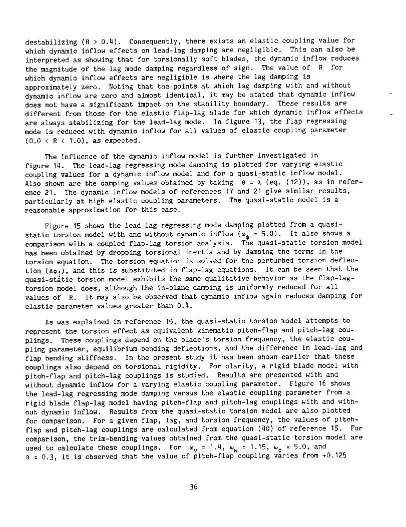
destabilizing (R > 0.4). Consequently, there exists an elastic coupling value for

which dynamic inflow effects on lead-lag damping are negligible. This can also be

interpreted as showing that for torsionally soft blades, the dynamic inflow reduces

the magnitude of the lag mode damping regardless of sign. The value of R for

which dynamic inflow effects are negligible is where the lag damping is

approximately zero. Noting that the points at which lag damping with and without

dynamic inflow are zero and almost identical, it may be stated that dynamic inflow

does not have a significant impact on the stability boundary. These results are

different from those for the elastic flap-lag blade for which dynamic inflow effects

are always stabilizing for the lead-lag mode. In figure 13, the flap regressing

mode is reduced with dynamic inflow for all values of elastic coupling parameter

(0.0 < R < 1.O), as expected.

The influence of the dynamic inflow model is further investigated in

figure 14. The lead-lag regressing mode damping is plotted for varying elastic

coupling values for a dynamic inflow model and for a quasizstatic inflow model.

Also shown are the damping values obtained by taking 8 = _ (eq. (12)), as in refer-

ence 21. The dynamic inflow models of references 17 and 21 give similar results,

particularly at high elastic coupling parameters. The quasi-static model is a

reasonable approximation for this case.

Figure 15 shows the lead-lag regressing mode damping plotted from a quasi-

static torsion model with and without dynamic inflow (_ = 5.0). It also shows a

comparison with a coupled flap-lag-torsion analysis. The quasi-static torsion model

has been obtained by dropping torsional inertia and by damping the terms in the

torsion equation. The torsion equation is solved for the perturbed torsion deflec-

tion (A¢]), and this is substituted in flap-lag equations. It can be seen that thequasi-static torsion model exhibits the same qualitative behavior as the flap-lag-

torsion model does, although the in-plane damping is uniformly reduced for all

values of R. It may also be observed that dynamic inflow again reduces damping for

elastic parameter values greater than 0.4.

As was explained in reference 15, the quasi-static torsion model attempts to

represent the torsion effect as equivalent kinematic pitch-flap and pitch-lag cou-

plings. These couplings depend on the blade's torsion frequency, the elastic cou-

pling parameter, equilibrium bending deflections, and the difference in lead-lag and

flap bending stiffness. In the present study it has been shown earlier that these

couplings also depend on torsional rigidity. For clarity, a rigid blade model with

pitch-flap and pitch-lag couplings is studied. Results are presented with and

without dynamic inflow for a varying elastic coupling parameter. Figure 16 shows

the lead-lag regressing mode damping versus the elastic coupling parameter from a

rigid blade flap-lag model having pitch-flap and pitch-lag couplings with and with-

out dynamic inflow. Results from the quasi-static torsion model are also plotted

for comparison. For a given flap, lag, and torsion frequency, the values of pitch-

flap and pitch-lag couplings are calculated from equation (40) of reference 15. For

comparison, the trim-bending values obtained from the quasi-static torsion model are

used to calculate these couplings. For _v = 1.4, _w = 1.15, me = 5.0, and

0 = 0.3, it is observed that the value of pitch-flap coupling varies from +O.125

36

for _ = 0.0 to -0.414 for R = 1.0. The pitch-lag coupling varies from -1.4602

for R = 0.0 to -1.497 for R = 1.0. Comparing the curves for both the models with

no dynamic inflow, it can be seen that the rigid blade model yields conservative

results. With dynamic inflow, both models qualitatively exhibit the same trend,

namely, that a reduction in damping results with increasing elastic coupling for

R > 0.5. It may be concluded from figures 15 and 16 that a rigid blade flap-lag

model with pitch-flap and pitch-lag couplings, rather than a model with coupled

flap-lag-quasi-static torsion for full flap-lag-torsion, may in some cases be suffi-

cient to yield qualitative trends.

Summary of Hover Study

The combined effect of blade torsion and dynamic inflow on the aeroelastic

stability of an elastic rotor blade in hover has been studied. The governing equa-

tions of motion of the elastic blade with flap-lag-torsion degrees of freedom and

the dynamic inflow equations are derived using a symbolic processor written in

FORTRAN. The blade and the dynamic inflow equations are converted to equations in a

multiblade coordinate system by rearranging the coefficients of the equations.

Conclusions drawn from this study are presented in the last section of this report.

Forward Flight

In forward flight the rotor does not have an axisymmetry flow environment as it

does in hover. The velocities of the rotor blade not only depend on the blade

motion and on rotational speed but also on the on-coming air speed. These addi-

tional components of air velocity are shown in figure 17. The advancing blade has a

velocity relative to the air higher than the rotational velocity, whereas the

retreating blade has a lower velocity relative to the air. The aerodynamic forces

vary periodically as the blade rotates. This causes asymmetry of the loads. The

rotor blade loading and motion are periodic with a fundamental frequency equal to

the rotor speed _. The analysis is more complicated because of the dependence of

the loads and motion on the azimuth angle _. A phenomenon which can be introduced

by forward flight is the reverse-flow region, an area on the retreating side of the

rotor disk where the velocity relative to the blade is directed from the trailing

edge to the leading edge. In general, the reverse-flow region is defined as the

area of the disk where the tangential velocity is less than zero, which has the

boundary x + _ sin @ = O. This yields a circular region with a diameter _, cen-

tered at x = _/2, and _ = 270 deg on the retreating side. Aeroelastic studies in

forward flight are consequently more complex than are hover studies. The governing

equations are lengthy and have periodic coefficients. However, as in hover,

reliable solutions can be obtained by linearizing the nonlinear equations about a

steady-state equilibrium position. In forward flight this position is a time-

dependent periodic solution. Calculation of this time-dependent equilibrium posi-

tion is inherently coupled with the trim state of the complete helicopter in forward

flight.

Formulation of forward flight stability analysis- The blade model remains the

same as described for hover and shown in figure 2. The blades undergo axial (u),

37

lagwise benging (v), and flapwise bending (w) and torsion deflection (_). Theaerodynamic forces will have additional contributions from the airspeed. Thesecontributions have been shown in figure 17. The general formulation of the problemfollows the sameprocedure as the one for hover. However, in forward flight theimplementation of Galerkin's method requires the rotating modesto be calculated atevery instant of time for a given pitch. It is proposed here to derive the govern-ing equations of motion using the uncoupled rotating modes evaluated at zeropitch. The elastic degrees of freedom v, w, and _ are expressed in terms of thegeneralized coordinates and modeshape functions as

NF

w : _ Rwi(_)ni(_)

i=I

NL

v : _ Rvi(@)_i(x)

i=I

NT

: _ _i(_)ei(_)

i=I

(23)

, - . are rotating mode shapes; NF, NL, and NTwhere @ : _t x : x/R, hi, _i' and eare the number of flap, lag, and torslon modes used in the analysis. These mode

shapes are obtained from five nonrotating modes for each degree of freedom. In the

actual derivation of the equations through HESL, the integral quantities are evalu-

ated by the numerical program using these modes. Two rotating modes are used in

this study for each flap, lag, and torsion degree of freedom.

Equations through HESL- The derivation of the governing equations of motion for

a single blade using HESL is the same as described for hovering flight. The only

change in data input is the air velocity components which are caused by the air

speed. The data for the position vector, strain expressions, air velocity compo-

nents, and transformation matrices from reference 24 are given as the basic data.

The displacements as given in terms of the generalized coordinates (eq. (23)) are

substituted and the equations are derived using a Lagrangian approach. The per-

turbed equations are obtained by substituting the relations given by equation (8).

The nonlinear single blade equations are written to a separate file, to be used in

the time-dependent equilibrium position calculation. The perturbed equations are

similarly written to a file to be used in a multiblade coordinate transformation.

The relations required in dynamic inflow calculations, thrust (CT) , pitching moment

(CM) , and rolling moment (CL) are derived using the perturbed aerodynamic force in

the flap direction. The equations are lengthy because of the contributions from

airspeed. The program generates the steady and perturbed equations in a single

38

operation and outputs them individually. This is convenient in the case of forward

flight not only because of the large number of terms present in each equation, but

also for the different analysis processes that are required for the steady and

perturbed sets of equations.

In the present study, the order of the variables and the ordering scheme used

are same as those followed in reference 15. All the o(_ 2) terms, when compared

to o(I), except those that contribute.to._ead-lag and torsion damping areneglected. Nonlinear rate products (vw, v , etc.) are retained since they contrib-

ute to the linearized stability analysis. Although any general ordering scheme

could have been used to obtain the final equations of motion, this ordering scheme

is considered representative and adequate for demonstrating the capability of the

symbolic analysis process. For the results presented here, it took approximately

300 sec to symbolically derive both the structural and aerodynamic equations on a

VAX 11/780 computer. It should be noted that for a hingeless rotor, the axial

displacement can be solved for a priori as a function of flap and lag bending. In

this report, expressions for axial dlspIacement and axial velocity are taken from

reference 15 and supplied as data to the program.

Dynamic inflow modeling- The dynamic inflow equations are related to the blade

degrees of freedom through the variations in thrust, pitching and rolling moments

[m] vc ÷ [£]-I : CM

Vc CL-_S _, V S

(24)

The elements of (m) and (£) define the various dynamic inflow models that can be

included in an analysis. Reference 19 presents a hierarchy of models, having dif-

ferent elements for (m) and (£) from actuator disk theory in forward flight. The

elements of (£) depend on the wake skew angle at the rotor

mR : tan - (25)

where _ is the steady inflow. Of the 13 models presented in reference 19, the

partially constrained model gave good results. In the present report, this par-

tially constrained theory is used to obtain the dynamic inflow results. The ele-

ments of (m) and (£) are given by

128 -16m11 - 75 _ ' m22 : m33 : 4-_- _ ' mi_J : 0 , i _ j

!

I 15__/I - sin mR -4

£11 : 2 ' £13 : _-V1 + sin mR ' £22 : I + sin mR (26)

39

-4 sin o R

g31 = £13 ' _33 : I + sin oR ' _12 = _21 = _23 = _32 = 0

I- E _ =

_iJ _ ij '

[ 2 + [ (2[ - p tan a)]

Trim and periodic equilibrium solution- The nonlinear periodic coefficient

equations obtained earlier can be solved for the periodic response in the time

domain using a Floquet method or in the frequency domain using a harmonic balance

method. Either will yield the time-dependent equilibrium position about which the

nonlinear equations can be linearized for an eigensolution. In forward flight, this

equilibrium position is coupled with the entire trim state of the helicopter. The

trim state is the steady state condition achieved by the system as time increases

without bound with the controls fixed and no external output present. Calculation

of a trim position requires establishing the control settings for a given flight

condition. The control settings are collective pitch, longitudinal and lateral

cyclic pitch, and the rotor shaft angle of attack. The induced velocity which

depends on the generated thrust and advance ratio is also calculated. In this

report, the harmonic analysis method coupled with an iteration on the trim state is

employed to calculate the equilibrium position and the trim settings. This numeri-

cal procedure, taken from reference 26 is as follows. An iterative inner loop in

which the solution for the periodic motion is obtained with fixed values of the trim

variables is nested within an outer loop in which the solution for the trim varia-

bles is obtained. The rotorcraft motion is solved for the periodic motion by the

harmonic analysis method which directly calculates the harmonics of a Fourier series

representation of the motion. The procedure advances the rotor around the azimuth

calculating the forcing functions in the time domain and then updating the harmonics

of the response. The forces and moments acting on the rotor are calculated from

this response, and the controls are adjusted until the equilibrium of forces and

moments that are required for the specified operating state is achieved.

For the harmonic analysis method, the governing equations of motion are written

with all the time-dependent and nonlinear terms as a forcing function, as

[.]{x}÷ + [K]{x}: (27)

where matrices M, C, and K are the constant parts of the mass, damping and stiff-

ness matrices, and where X is the vector of degrees of freedom. The function F

is evaluated at J points around the rotor azimuth

Fj = F(_j) (28)

40

and the harmonics of a complex Fourier series representation of F are given by

J

-in_jI e

Fn:_ Fj

J:1

(29)

Then the nth harmonic of the motion is given by

x : H-IF (30)n n n

where H = K - n2M + iCn. The iterative solution proceeds as follows. At a given

azimuth $j, the blade motion is calculated using the current estimates of theharmonics

L

X : _. Xn ein_j

n:-L

(31)

Lin_j

X=_ Xne

n= -L

where L is the number of terms used in the expansion of X. The forcing function

is evaluated with this motion. Then the change in the harmonics caused by the

change in the forcing function is calculated and added to the harmonics calculated

in the last revolution. After every revolution the old and new harmonics are

checked until convergence is achieved.

After obtaining the harmonics of the blade motion, the equilibrium of the rotor

forces and moments is checked. If overall equilibrium is not satisfied, the trim

settings are changed and the procedure is repeated until equilibrium is obtained.

The following assumptions are made in arriving at the equilibrium of the forces and

moments. The helicopter is in straight and level steady flight, the rotor hub

moments are trimmed to zero with fuselage and other aerodynamic contributions

neglected. Then the equilibrium of forces and moments are given by

w

CT cos u + CH sin _ : CW 7

-CT sin u + CH cos _ = -CX

=C =0.0Cmx my

(32)

where Cx : (I/2)fw 2 and _ is the shaft angle of attack.

41

In calculating thrust, horizontal force, and the hub moments, the steady inflow

appears as a parameter which in turn depends on the rotor thrust and shaft angle of

attack. In this study, the study inflow is taken as an equation of constraint and

solved along with the four equations above.

k - _ tan _ - (x + _ = 0.0 (33)

The increments in the trim settings are calculated using a modified Newton-Raphson

method (ref. 30). If v is the control variable and M is the target to be

achieved, then a first-order approximation of M(v) is

-I

Mtarget = Mn+ I = M n + (Vn+ I - vn) or Vn+ I = v + D (Mtarget - Mn)f (34)

where vn and Vn+ I indicate the current and new estimates of v respectively and

f < I is included to avoid overshoot oscillations in the trim iteration by reducing

the step size. The partial derivative matrix D is

oM[M ][M viMvivi]_v .... _v i Av. (35)i

where v i is the ith control variable and Av i is its increment. The conver-

gence is checked when the tolerence level as specified by the parameter E is

met. For more details on this procedure see reference 30. In the present study,

all the degrees of freedom, blade flap, lead-lag and torsion degrees of freedom are

used in calculating the trim state and periodic response.

The periodic response can also be obtained using Floquet methods (ref. 16). A

review of these methods to obtain the initial conditions, forced response and sta-

bility data is given in reference 31. Explicit harmonic balance equations can also

be derived symbolically using the program HESL. This requires the definition of the

harmonics for each degree of freedom and a table of trigonometric relations giving

the products of sines and cosines as sums of sines and cosines. Then the SUBSTITUTE

TABLE INTO RELATIONS command substitutes these relations into the governing equa-

tions. A numerical program collects the coefficients of sines and cosines and forms

the harmonic balance equations. However, this procedure requires modification of

the data for each degree of freedom when a larger number of harmonics is involved.

Hence, HESL is not convenient to use to derive explicit harmonic balance equations

and numerical method as explained above is employed in this study.

Aeroelastic stability solution (single blade)- Once the time dependent equilib-

ri_ position is determined, the nonlinear equations are perturbed about this equi-

librium position, equation (8). As mentioned earlier, the symbolic program gener-

ates the perturbed equations and writes them into subroutines. It should be noted

that squares of the perturbation quantities are typically neglected by the symbolic

42

program when employing a realistic ordering scheme. The final system of equations

for stability is

tp1{A }÷ ÷ [RJ{Aq}:0 (36)

or

:[As]Z

The stability of this linearized system is determined from Floquet theory by

evaluating the characteristic exponents of [As]

kk = _k + iUk (37)

The mass, damping and stiffness terms are identified by a numerical program for each

time step. The linearized system is stable when _k < O.

Multiblade coordinate transformation- It is necessary to convert the equations

into a fixed coordinate system to provide a better understanding and to include

dynamic inflow effects which are referenced to the fixed system. The multiblade

(Fourier) coordinate transformation is a linear transformation of the degrees of

freedom from the rotating to nonrotating frame. In the case of hovering flight,

this transformation has been easily performed by rearranging the coefficients of the

equations, since the coefficients are constant. For forward flight the coefficients

are periodic. Hence the multiblade coordinate transformation is more complicated.

Let X be a generalized degree of freedom (dimensionless) in the rotating frame for

the ith blade. Then for a three-bladed rotor, the relations

Xi : XO + Xc cos _i + Xs sin ti

Xi : Xo + (Xc + Xs)C°S _i + (Xs - Xc)sin _i (38)

Xi : XO + (Xc + (Xc + 2Xs - Xc)C°S _i + (Xs - 2Xc - Xs)sln #i

give the ith generalized blade degree of freedom using multiblade coordinates in

the nonrotating frame. The variables Xo, Xc, and Xs are the rotor degrees of

freedom, and they describe the motion of the rotor as a whole in the nonrotating

frame.

The Multiblade Coordinate Transformation involves the following steps

(ref. 29): (I) expansion of each degree of freedom into multiblade coordinates;

(2) multiplication of the resulting expression with multiblade functions I, cos _,

sin _, cos 2_, sin 2_, etc., depending on the number of blades; (3) replacement of

products of sines and cosines as sums of sines and cosines using trigonometric

relations; and (4) deletion of terms which are not periodic multiples of the number

of blades (summation rules). Using the symbolic program, this is achieved as fol-

lows. The multiblade expansion of each degree of freedom and its time derivative is

given as a table of relations (eq. (38)). The multiblade functions I, cos #,

43

sin _, cos 2_, sin 2_, etc., required in transforming the equations, are read as

data (or can be generated within the program). The trigonometric relations giving

the product of sines and cosines as sums of sines and cosines are given as a table

of relations. This requires that the equation derivation consist of several runs

until all the required relations are included in the table of relations without

exception. Then the command PERFORM MULTIBLADE TRANSFORMATION multiplies the equa-

tion with each of the multiblade functions, substitutes the multiblade expansion for

each degree of freedom, substitutes the trigonometric relations (from the given

tables of relations), and checks for the multiples of the blade harmonics. Only

terms which contain a periodic multiple of number of blades are retained. The

interface routines separate the terms into constant and periodic parts (coefficient

of each harmonic separately), and writes them into subroutines. In this manner, the

constant coefficient approximation is easily done. In this study the perturbed

governing equations of motion and perturbations in thrust and in moment equations

are converted into multiblade coordinate equations. The multiblade solution was

subsequently checked for accuracy by comparing results with a single blade solution

without dynamic inflow. It should be noted that the trim value harmonics entering

as nonlinear contributions should be defined as symbolic data. The input data

increase as more nonlinear terms are taken into account. These data are in addition

to the data given for the multiblade expansion of the degrees of freedom. However,

the output may be smaller since only terms which are multiples of the number of

blades are retained. Since this is a feasibility study to obtain explicit multi-

blade equations using a symbolic program in FORTRAN, the nonlinear quantities are

assumed to provide only first harmonic forcing contributions. For the results

presented here, the program was run on a VAX 11/780 computer. For each equation, it

took approximately 250 sec to derive the multiblade equations and 120 sec to write

these into subroutines for numerical analysis.

From the amount of input required to perform a symbolic formulation of the

harmonic balance and multiblade equations, the program HESL is convenient to explic-

itly consider the symbolically derived equations only if the number of degrees of

freedom are small. As pointed out in reference 29, numerical schemes are better

suited for general models so that the harmonic balance equations and multiblade

equations can be efficiently obtained after obtaining the steady and perturbed

equations from the symbolic program.

The symbolic program separates the terms containing the periodic variable

cos Nt and sin Nt and writes the equation as

A(t) : A0 + AN cos Nt + BN sin Nt (39)

In subroutine form they are referred to as A(1), A(2), and A(3). This allows for

direct elimination of the matrices A(2) and A(3) for a simple constant coefficient

analysis.

Aeroelastic stability solution (multiblade and dynamic inflow)- The final gov-

erning equations of motion can be written as

44

[P]{q} + [Q]{(]} + [R]{q} + [T]{u} = 0 (40a)

for the blade equations, and

[A]{_}÷ [B]{_}÷ [C]{q}÷ [G]{u}: m{a}÷ [_]-_{u}

for the dynamic inflow equations, where {q} is {qo' qc' qs } ' qo

collective modes, qc is vector of all lateral cyclic modes, qs

longitudinal cyclic modes, and {u} is (_O,_c,_s).

Equations (40a) and (4Ob) can be combined as

{x}÷A B (G - _-I ]{_}+[R _]{X}C

(40b)

is vector of all

is vector of all

where

The final stability equations in state vector form are

: O (41)

where

{_}= [As]{Y} (42)

The stability results are obtained by calculating the eigenvalues of [As] , in a

similar manner to the single blade case.

The size of the state matrix depends on the number of modes and blades. For

the flap-lag-torsion model with two modes each, the size of the state matrix is

36 x 36 without dynamic inflow and 39 x 39 with dynamic inflow. The corresponding

values for a flap-lag model are 24 x 24 and 27 x 27, respectively.

Results and discussion- Results are presented for a uniform blade with zero

built-in twist, zero blade offsets, and zero precone angle. Reversed flow effects

are neglected. A three-bladed rotor is considered. Two rotating modes for each

flap, lag, and torsion degrees of freedom are used in the calculations. These modes

are calculated at zero pitch and are obtained from five nonrotating modes. Results

for both a single blade solution and a multiblade solution are presented for differ-

ent blade structural models. All results are for a propulsive trim condition,

calculated for a specified weight coefficient of Cw = 0.007 and an equivalent drag

45

area D/q = f = 0.012(_R2), where D is the drag force and q is the dynamic

pressure.

In the derivation of the equations, the orders of magnitude assigned for each

parameter are the same as that which followed in reference 15. The other parameters

used for the numerical study are

_v = 0.7, 1.4 , _w = 1.15 , _ = 3.0 , c/R = 0.07854 , y = 5.0 ,

a = 0.1 , a = 2_ , Cd = 0.01 , 8pc = 0.0 ,O

Kml/Km2 = O.0 ,

Km/R : 0.025, (KA/Km)2 = 1.5

Lead-lag damping values (real part of the characteristic exponent) are pre-

sented for a soft in-plane and stiff in-plane rotor with and without dynamic

inflow. The results present an investigation of: (I) the effect of degrees of

freedom used in the trim analysis on the lead-lag damping, (2) the effect of using

only one torsion mode, (3) the inclusion of a dynamic inflow model, and (4) the

difference between periodic and a constant coefficient approximation (where all

time-dependent coefficients are neglected).

_nfluence of trim analysis. The effect of the number of degrees of freedom

used in the trim analysis on the lead-lag damping is investigated in figures 18

and 19. Figure 18 shows the lead-lag damping plotted versus advance ratio for a

soft in-plane rotor (_v = 0.7). It can be seen that a flap-lag-torsion stability

analysis from a flap trim analysis underpredicts the lead-lag damping. The second

mode shows the same trend with the difference in predicted damping increasing with

advance ratio. Figure 19 shows the lead-lag damping plotted for a stiff in-plane

rotor (_v = 1.4) as a function of advance ratio. The results also show an increase

in damping when a flap-lag-torsion trim analysis is used. It is also noted that at

an advance ratio of 0.37 < _ < 0.41, the roots separate, and one root becomes less

stable whereas the other becomes more stable. The damping does reduce as the

advance ratio is increased beyond _ = 0.37. The second mode remains stable at all

advance ratios considered.

The increase in damping observed above for both soft in-plane and stiff

in-plane rotors is due to the different time-dependent equilibrium positions that

are used to linearize the full nonlinear equations. A full flap-lag-torsion trim

analysis is consistent in that the blade model has the same degree of complexity in

both the trim and in the stability analysis. It should be noted qualitatively that

the same type of trend is observed in reference 16, for both soft in-plane and stiff

in-plane rotors. This verifies the symbolic and numerical programs for the single

blade results and forms the basis to check the symbolically derived explicit multi-

blade equations (and numerical results) presented in the next section.

Influence of elastic torsion model. Figures 20 and 21 present the lead-lag

damping plotted versus advance ratio from a flap-lag model, flap-lag-torsion model

46

(two modes each), and flap-lag-torsion model with only one torsion mode, for a soft

in-plane rotor (mv = 0.7) using a single blade analysis. Figure 20 presents the

damping results for full elastic coupling (R = 1.0). It can be seen that the flap-

lag model underpredicts the lead-lag damping. The model with only one torsion mode

increases the damping above the model with two modes each. Figure 21 shows the

lead-lag damping value plotted for zero elastic coupling (R = 0.0). The damping

levels are much reduced when they are compared with the full elastic coupling

case. However, the flap-lag model is again lowest damped.

Lead-lag damping is plotted for a stiff in-plane rotor (_v = 1.4) with varying

advance ratio in figures 22 and 23. Figure 22 presents the damping results for full

elastic coupling. The same trend that was observed for the case of a soft in-plane

rotor (fig. 6) exists. Note that root splitting for high-advance ratios occurs even

when only one torsion mode is used.

Figure 23 presents the lead-lag damping for increasing advance ratio for a

stiff in-plane rotor for a zero elastic coupling parameter and as a result, the

rotor is unstable. However, a flap-lag model predicts a stable system. This demon-

strates the importance of elastic blade torsion in the analysis.

Lead-lag damping is plotted in figure 24 for an advance ratio of _ = 0.25

while varying the elastic coupling parameter for a stiff in-plane rotor. Here a

flap-lag model predicts positive damping for all values of R, whereas for a flap-

lag-torsion model, the damping varies with elastic coupling parameter, increasing

with elastic coupling parameter.

Multiblade equation results. The following figures present the lead-lag

regressing mode damping results obtained using multiblade equations. The multiblade

equations are explicitly derived using the symbolic program. This required explicit

definition of all nonlinear contributions and degrees of freedom in terms of their

harmonics. This significantly increased the amount of data that is required by the

symbolic program. Since this is a feasibility study on the use of symbolic programs

in FORTRAN, only first harmonics were considered in the nonlinear contributions.

Consequently, damping data determined from the multiblade equations may slightly

differ from the single-blade solution. Additionally, the multiblade results are

obtained by retaining only one torsion mode; however, the nonlinear contribution

from both torsion modes is used. This reduces the time step and time for integra-

tion in performing the Floquet-analysis.

The damping values are first checked with those obtained from a single-blade

solution obtained earlier to validate the multiblade equation derivation process.

It was found that the approximation cos e = 1.0, used in deriving the explicit

multiblade equations, will predict slightly higher (yet less than 2%) damping for

stiff in-plane rotors with a full elastic coupling parameter, since this approxima-

tion most greatly affects the coupling elements. For all other values of the elas-

tic coupling parameter, this approximation does not affect the damping value. Where

required for comparison, the single-blade damping values are recalculated using this

approximation, to avoid the rederivation of the multiblade equations.

47

Figures 25 and 26 show the lead-lag regressing modedamping plotted for varyingadvance ratio with and without dynamic inflow from a flap-lag-torsion and flap-lagmodel for a soft in-plane rotor. Figure 25 shows the damping for full elasticcoupling (R = 1.0). For the flap-lag-torsion model, the dynamic inflow reduces thedamping at all advance ratios. Its effect is almost negligible at advance ratios0.15 to 0.25. For the flap-lag model, the dynamic inflow increases the damping upto an advance ratio of 0.33, it then reduces the damping. Figure 26 presents thedamping results for the zero elastic coupling (R = 0.0). It is seen that for theflap-lag-torsion model, the dynamic inflow again reduces the damping in hover. Yetat intermediate advance ratios, dynamic inflow increases the damping, and at higheradvance ratios, it once again reduces the damping. For the flap-lag model, thedynamic inflow increases lead-lag damping for all the advance ratios that are con-sidered. This is consistent with previous studies, for example, as in reference 18.

The lead-lag regressing modedamping is plotted for a stiff in-plane rotor forvarying advance ratio in figures 27 and 28. Figure 27 is for a rotor with fullelastic coupling. For a flap-lag-torsion model, the dynamic inflow reduces thedamping up to an advance ratio of 0.41. For u > 0.41, this model shows a slightlyincreased damping value. The flap-lag model with dynamic inflow shows a smalldecrease in damping, yet this damping increment gets smaller with higher advanceratios. Figure 28 is for a rotor with zero elastic coupling. For this configura-tion, the dynamic inflow increases damping for all advance ratios. Consequently,both flap-lag-torsion and flap-lag models show the same trend.

Figure 29 shows the lead-lag regressing modedamping as it is plotted for astiff in-plane rotor at an advance ratio of 0.25 while varying the elastic couplingparameter. For the flap-lag-torsion model, dynamic inflow reduces the damping forR > 0.3; however, it increases the available damping for R < 0.3. This increase isnot sufficient to stabilize the in-plane mode. With the flap-lag model, dynamicinflow shows an increase in damping for all values of elastic coupling.

Constant coefficient approximation. The effect of a constant coefficientapproximation is studied in figure 30, where the real part of the exponent isplotted for a stiff in-plane rotor with full elastic coupling which showeda split-ting of the roots whenanalyzed with a full periodic coefficient. The constantcoefficient approximation does not show this splitting, since the frequencies areaway from the real axis. For this analysis, the regressing and collective modesdopredict the samedamping trend with advance ratio as shown by a full Floquet analy-sis. However, the progressing mode shows poor agreement between a constantcoefficient approximation analysis and a Floquet theory analysis. This is becausethe constant coefficient approximation can only be good for low frequency modes.

III. CONCLUSIONS

A symbolic manipulation program written in FORTRANis used to derive the aero-elastic analysis equations of an elastic blade with flap-lag-torsion degrees of

48

freedom in hover and in forward flight. A study is madeof the feasibility of usingthe program to obtain explicit equations in a harmonic balance method and to obtainmultiblade equations. Numerical results are presented for a flap-lag-torsion modeland for a flap-lag model with and without dynamic inflow for a propulsive-trimmedrotor. Both soft in-plane and stiff in-plane rotors are considered.

The following conclusions are drawn from using a symbolic program:

I. The program HESL,written in FORTRAN,can be conveniently used to deriveelastic blade equations.

2. The process of aeroelastic stability analysis starting from equation deri-vation to numerical calculation can be automated.

3. With the present program capability, the amount of data to the symbolicprogram increases rapidly with degrees of freedom and the number of harmonics thathave been analyzed.

4. In deriving the explicit harmonic balance equations and multiblade equa-tions, the following should be noted:

(a) To obtain the harmonic balance equations, a numerical method is sug-gested since an arbitrary number of harmonics can be used without increasing theinput data to the symbolic program.

(b) To obtain the multiblade equations, the perturbed equations in theirFourier series form are derived using the symbolic program. Then the multibladeequations themselves are obtained numerically.

It is recommendedthat a selective combination of the symbolic and numericalprograms is required for the derivation and numerical study to be efficiently con-ducted.

The following conclusions are drawn from the numerical study performed for ahovering rotor.

I. The unsteady aerodynamic effects on lag regressing modedamping, modeled asdynamic inflow, are dependent on the elastic coupling parameter for torsionallyflexible blades. For zero elastic coupling, dynamic inflow increased the lagregressing modedamping. For other elastic coupling parameter values, dynamicinflow either increased or decreased lag regressing modedamping.

2. Use of a quasi-static torsion blade model is conservative, and yields thesametrend with varying elastic coupling parameter as flap-lag-torsion model.

3. Whencomparedwith a flap-lag model, it is seen that the relationshipbetween dynamic inflow and lag regressing modedamping can be a result of the effectof pitch-flap and pitch-lag couplings, which depend on the elastic couplingparameter.

49

The following conclusions are drawn from the numerical study of a single bladesolution in forward flight.

I. A flap-lag-torsion stability analysis from a trim procedure where only theflap degree of freedom is used underpredicts the lead-lag damping.

2. In the case of stiff in-plane rotors, high-forward flight speed is desta-bilizing. At high advance ratios, a splitting of the roots is encountered whichyields two real values at the samefrequency.

3. Using only one torsion mode increases the damping value from the flap-lagstructural model.

4. The damping values for a stiff in-plane rotor are sensitive to elasticcoupling parameter.

The following conclusions are drawn from the numerical study of a multibladesolution with dynamic inflow in forward flight.

I. For a flap-lag model, for both soft in-plane and stiff in-plane rotors,with zero elastic coupling, the dynamic inflow increased damping at all advanceratios considered; with full elastic coupling the dynamic inflow increased thedamping at low-advance ratios, but reduced damping at high-advance ratios.

2. For a flap-lag-torsion model, dynamic inflow slightly reduced lead-lagregressing modedamping for all advance ratios. The sametrend is observed for bothsoft in-plane and stiff in-plane rotors.

3. For a given advance ratio, the variation of damping with an elastic cou-pling parameter for a stiff in-plane rotor showed the same trend as it did for thehover case.

4. The constant coefficient approximation for the stiff in-plane rotor doesnot show the splitting of the rotors, since the frequency of the lag mode is awayfrom the real axis.

5O

APPENDIXA

This appendix shows the input data (Table AI) and the output data (Table A2)

from the symbolic program to derive flap equations for a rigid rotor blade. The

problem definition starts with a flap-lag transformation but is subsequently reduced

to flap model. This simplified model is used to clarify the program aspects rather

than the modeling aspects. Even though the data is given at the matrix level to

show that the symbolic program is capable of handling matrices, in this example it

is simple to use the definition of the position vector directly as input. Both the

single blade and multiblade equations for a three-bladed rotor are obtained from the

symbolic program.

Table A3 gives the FORTRAN symbols used to define the original variables.

51

TABLE AI.- INPUT TO THE PROGRAM HESL TO OBTAIN LINEARIZED FLAP EQUATION AND

MULTIBLADE EQUATIONS FOR THREE-BLADED ROTORS

%@#READ MATRIX

#TFLPO303O1

I.0 COSB

O1

O.OO1

-I .O SINB

01

0.O

O1

1.O

O1

O.O

O1

I.0 SINB

O1

O.O

O1

1. O COSBREAD MATRIX

#TLAGO30301

1.0 COSZ

O1

-I .O SINZ

01

O.O

O1

I.O SINZ

O1

I.O COSZ

01

0.O

01

0.O

01

0.O

01

1.O

READ MATRIX

#POVE0301011.0 RB010.001

52

TABLE AI.- CONTINUED

0.0

READ DIFERENTIATION TABLE

@DERVIO

BT BTO I

1.0

BTD BTDO I

1.0

BT COSBO I

-I .0 SINB

BT SINBO I

I.0 COSBTAU BTO I

I.0 BTDTAU BTDO I

I.0 BTDDTAU COSBO I

-I.0 SINB BTD

TAU SINB01

I.0 COSB BTDTAU CSCYO I

-I.0 SNCY

TAU SNCYO I

I.0 CSCY

READ TABLE FOR SUBSTITUTION

&SUPR02

01 SINZ01

0.0

01 COSZ01

1.0READ TABLE FOR SUBSTITUTION

@DUMYO I0102 SINB02

1.0- I.0 COSB COSB

READ TABLE FOR SUBSTITUTION

@DUM I01

01 ABCD01

1.0

READ TABLE FOR SUBSTITUTION

@INRL0301

01 RB02

I.0 IB

01 RB01

I.5 IB

01 RBO0

3.0 IBREAD TABLE FOR SUBSTITUTION

@PERT0502 BTDDO I

I.0 BBDD

I.0 DBDD

53

TABLEAI.- CONTINUED

02 BTDO I

I.0 BBD

I.0 DBD

02 BTO I

I.0 BB

I.0 DB

02 SINBO I

1.0 BB

I.0 DB

01 COSB01

1.0READ VARIABLES FOR COLLECTION OF COEFFICIENTS

@MUCF12THO THI TH2 BDDO BDDI BDD2 BDO BDI BD2

READ TABLE FOR SUBSTITUTION

@MULB04

07 DBDDO II.0 BDDO

I.0 BDD I CSCY

-2.0 BDI SNCY

-I.0 BI CSCY

I.0 BDD2 SNCY

2.0 BD2 CSCY

-I.0 B2 SNCY

05 DBD01

I.0 BDO

I.0 BD I CSCY

-1.0 BI SNCY

I.0 BD2 SNCY

I.0 B2 CSCY

03 DB01

I.0 BO

I.0 BI CSCYI.0 B2 SNCY

03 THTAO I

I.0 THO

I.0 TH I CSCYI.0 TH2 SNCY

READ TABLE FOR SUBSTITUTION

@TRIG120102 SNCY02

0.5

-.5 C2CY

01 SNCY01 CSCY01

O.5 S2CY

02 CSCY02

0.5

O.5 C2CY

02 SNCY03

O.75 SNCY

-.25 S3CY

BO BI B2

54

TABLEAI.- CONTINUED

02 SNCY02CSCY01O.25 CSCY-. 25 C3CY02 SNCY01CSCY02O.25 SNCYO.25 S3CY02 CSCY03O.75 CSCYO.25 C3CY03 SNCY04O.375-0.5 C2CYO.125 C4CY02 SNCY03CSDY01O.25 S2CY-. 125 S4CY02 SNCY02CSCY02O.125-. 125 C4CY02 SNCY01CSCY03O.25 S2CYO.125 S4CY03 CSCY040.3750.5 C2CYO.125 C4CYFORMMATRIX#TLAG#TFLP#TFLGFORMMATRIX#TFLG#POVE#PVECMATRIXEXPRESSION03#PVEC% RI0101% R20201%R30301SUBSTITUTETABLEINTOEXPRESSION@SUPR%RI% RXSUBSTITUTETABLEINTOEXPRESSION@SUPR%R2% RYSUBSTITUTETABLEINTOEXPRESSION@SUPR5R3% RZREADEXPRESSION%OMEZOI1.0DIFERENTIATEEXPRESSION

TAU%RX%RXTDIFERENTIATEEXPRESSION

TAU%RY%RYTDIFERENTIATEEXPRESSION

TAU%RZ%RZTFORMEXPRESSION%RXD02I. 0 % RXT

55

TABLEAt.- CONTINUED

-1.0 % RY%OMEZ

FORM EXPRESSION

% RYD021.0 % RYT

1.0 %OMEZ% RXFORM EXPRESSION

% RZD01

1.0 % RZTREAD EXPRESSION

%SEBL01

0.5 KBT BTREAD EXPRESSION

%XVEL011.0 MU CSCY

READ EXPRESSION

%YVEL01-I.0 MU SNCY

READ EXPRESSION

%ZVEL01

-1.0 LAMD

FORM EXPRESSION

%AVLI021.0 %XVEL

-1.0 % RXDFORM EXPRESSION

%AVL202

1.0 %YVEL

-1.0 % RYDFORM EXPRESSION

%AVL3021.0 %ZVEL

-1.o _ RZDREAD MATRIX

#VXYZ03OI

O1

1.0 %AVLI

01

1.0 %AVL2

01

1.0 %AVL3

FORM MATRIX

#TFLP#VXYZ#VX2Y

MATRIX EXPRESSION02#VX2Y

% UT0201% U1P0301NEGATE EXPRESSION

% UTNEGATE EXPRESSION

01

BT

56

TABLE AI.- CONTINUED

0.501 RAC201

0.3333301 RAC201

0.2501 RAC201

1.0

% UIPSUBSTITUTE TABLE INTO EXPRESSION

@DUMY% UIP% UP

FORM EXPRESSION

% MB02

-0.5 % UT% UT THTA RAC2

0.5 % UT% UP RAC2 RBREAD TABLE FOR SUBSTITUTION

@DYNM040101RAC201 RB01

GAMI

RB02

GAMI

RB03

GAMI

RB

GAMI

DIFERENTIATE EXPRESSION

BTD% RXD%RXDQDIFERENTIATE EXPRESSION

BT% RXD% RXQDIFERENTIATE EXPRESSION

BTD% RYD%RYDQ

DIFERENTIATE EXPRESSION

BT% RYD% RYQDIFERENTIATE EXPRESSION

BTD% RZD%RZDQDIFERENTIATE EXPRESSION

BT% RZD% RZQREAD EXPRESSION

%CONS011.0

READ EXPRESSION

%CON I01-I .0READ VARIABLES FOR COLLECTION OF COEFFICIENTS

@PECF06DBDD DBD DB BBDD BBD BB

@INRL@DUMY@PERT

@INRL@DUMY@PERT

@INRL@DUMY@PERT

TAU@INRL@DUMY@PERT

TAU@INRL@DUMY@PERT

TAU@INRL@DUMY@PERT

BT@DUMI@DUMI@PERT

@DYNM@DUMY@PERT

INITIALIZE MULTIBLADE

03 MOPK CSCY SNCY C2CY S2CY C3CY S3CY C4CY S4CY C5CY S5CY C6CY S6CY C7CY S7CY

FORM LAGRANGIAN

O8O3OOO1OO

%SBEQSPECF*E2DI

% RXD% RXQ%CONI

% RYD% RYQ%CONI

% RZD% RZQ%CONI

% RXD%RXDQ%CONS

% RYD%RYDQ%CONS

% RZD%RZDQ%CONS

%CONS%SEBL%CONS

%CONS% MB%CONS

57

TABLEAt.- CONCLUDED

PERFORMMULTIBLADETRANSFORMATIONO3@MULTB@TRIG@MUCF%SBEQ%AEM1%AEM2%AEM3ENDOFDATA

58

TABLE A2.- SAMPLE OUTPUT

READ VARIABLES FOR COLLECTION OF COEFFICIENTS

RDCCVR DBDD DBD DB BBDD BBD BB

FORM LAGRANGIAN

* DETAILS OF THE EXPRESSION SBEQ *

* NUMBER OF TERMS 19 *

- GROUP OF TERMS WITH VARIABLE DBDD -

I 1.000" IB*

- GROUP OF TERMS WITH VARIABLE DBD -

I 0.167*SNCY* MU*GAMI*

2 0.125*GAMI*

- GROUP OF TERMS WITH VARIABLE DB -

I 1.000* KBT*

2 0.250*CSCY*SNCY* MU*

3 0.167"CSCY* MU*GAMI*

4 1.000* IB*

MU*GAMI*

- GROUP OF TERMS WITH VARIABLE BBDD -

I 1.000* IB*

- GROUP OF TERMS WITH VARIABLE BBD -

1 O.167*SNCY* MU*GAMI*

2 0.125*GAMI*

59

TABLE A2.- CONTINUED

- GROUP OF TERMS WITH VARIABLE BB -

1.0OO* KBT*

0.167"CSCY* MU*GAMI*

1.O00* IB*

0.250*CSCY*SNCY* MU* MU*GAMI*

- REMAINING TERMS IN EQUATION -

I

2

34

5

-0.250*SNCY*SNCY*THTA* MU* MU*GAMI*

-0.125*THTA*GAMI*

-0.333*SNCY*THTA* MU*GAMI*

0.250*SNCY* MU*LAMD*GAMI*0.167*LAMD*GAMI*

PERFORM MULTIBLADE TRANSFORMATION

MULTIBLADE EQUATION I

* DETAILS OF THE EXPRESSION AEMI *

* NUMBER OF TERMS 17 *

- GROUP OF TERMS WITH VARIABLE THO -

-0.375* MU* MU*GAMI*

-0.375*GAMI*

- GROUP OF TERMS WITH VARIABLE THI -

1 0.188"C3CY* MU* MU*GAMI*

- GROUP OF TERMS WITH VARIABLE TH2 -

0.188"$3CY* MU* MU*GAMI*

-0.500* MU*GAMI*

60

TABLEA2.- CONTINUED

- GROUPOFTERMSWITHVARIABLE BDDO -

I 3.000* IB*

- GROUPOFTERMSWITHVARIABLE BDO -

I 0.375*GAMI*

- GROUPOFTERMSWITHVARIABLE BD2 -

I 0.250* MU*GAMI*

- GROUPOF TERMSWITHVARIABLE BO -

I 3.000* IB*

2 3.000* KBT*

- GROUP OF TERMS WITH VARIABLE BI -

I 0.188"$3CY* MU* MU*GAMI*

- GROUP OF TERMS WITH VARIABLE B2 -

I -0.188"C3CY* MU* MU*GAMI*

- REMAINING TERMS IN EQUATION -

I

2

34

5

0.375* BBD*GAMI*

3.000* BB* KBT*

3.000* IB*BBDD*

3.000* IB* BB*

0.500*LAMD*GAMI*

61

TABLEA2.- CONTINUED

MULTIBLADEEQUATION 2

* DETAILSOFTHEEXPRESSIONAEM2 ** NUMBEROFTERMS 19 *

- GROUPOFTERMSWITHVARIABLE THO -

I 0.188"C3CY* MU* MU*GAMI*

- GROUPOFTERMSWITHVARIABLE THI -

I23

-0.094" MU* MU*GAMI*-0.188*GAMI*-0.250"$3CY* MU*GAMI*

- GROUPOFTERMSWITHVARIABLE TH2 -

I 0.250"C3CY*MU*GAMI*

- GROUPOFTERMSWITHVARIABLE BDDI -

1 1.500" IB*

- GROUP OF TERMS WITH VARIABLE BDI -

I

2

0.188*GAMI*

0.125"$3CY* MU*GAMI*

- GROUP OF TERMS WITH VARIABLE BD2 -

I

23.000* IB*

-0.125"C3CY* MU*GAMI*

62

TABLEA2.- CONTINUED

- GROUPOF TERMSWITHVARIABLE BO -

0.250* MU*GAMI*0.188"$3CY* MU* MU*GAMI*

- GROUPOFTERMSWITHVARIABLE BI -

1.500' KBT*0.250"C3CY* MU*GAMI*

- GROUPOFTERMSWITHVARIABLE B2

I

2

3

0.250"$3CY* MU*GAMI*0.188*GAMI*

0.094* MU* MU*GAMI*

m_

- REMAINING TERMS IN EQUATIONm_

I

2

0.188" BB*S3CY* MU* MU*GAMI*

0.250* BB* MU*GAMI*

MULTIBLADE EQUATION 3

,H***HH*H_H**HHHHHHHHHHH*H*H**MHHNH**HNH**

* DETAILS OF THE EXPRESSION AEM3 ** NUMBER OF TERMS 21 *

**************************_***************

- GROUP OF TERMS WITH VARIABLE THO -

I

2

0.188"$3CY* MU* MU*GAMI*

-0.500* MU*GAMI*

- GROUP OF TERMS WITH VARIABLE THI -

I 0.250"C3CY* MU*GAMI*

63

TABLEA2.- CONTINUED

- GROUPOF TERMSWITHVARIABLE TH2 -

I23

-0.281" MU* MU*GAMI*-0.188*GAMI*0.250"$3CY* MU*GAMI*

- GROUPOFTERMSWITHVARIABLE BDD2 -

I 1.500" IB*

- GROUPOFTERMSWITHVARIABLE BDO -

I 0.250* MU*GAMI*

- GROUPOFTERMSWITHVARIABLE BDI -

-3.000" IB*-0.125"C3CY* MU*GAMI*

- GROUPOF TERMSWITHVARIABLE BD2 -

I2

0.188*GAMI*-0.125"$3CY* MU*GAMI*

- GROUPOFTERMSWITHVARIABLE BO -

I -0.188"C3CY* MU* MU*GAMI*

- GROUPOF TERMSWITHVARIABLE BI -

I23

0.250"$3CY* MU*GAMI*-0.188*GAMI*0.094* MU* MU*GAMI*

64

TABLEA2.- CONCLUDED

- GROUPOFTERMSWITHVARIABLE B2 -

-0.250"C3CY* MU*GAMI*1.500" KBT*

- REMAININGTERMSIN EQUATION -

0.250* BBD* MU*GAMI*-0.188" BB*C3CY* MU* MU*GAMI*0.375* MU*LAMD*GAMI*

ENDOFDATA

65

TABLE A3.- SYMBOL DEFINITIONS

Symbol

A

cos ¢, cos 2_

cos 3¢, cos 4_

cos B, sin B

cos _, sin

Cdo/a

E

Is

K 8

r

sin _, sin 2_

sin 34, sin 4@

UT,U P

U I

VIeW t

8,B,S

80,81,82

80' 81' B2

SO,B1,B 2

U

e

e 0 ec,e S

FORTRAN Symbol Description

A

B,C

CSCY,C2CY

C3CY,C4CY

COSB,SINB

COSZ,SINZ

CDOA

E

IB

KB

RB

SNCY,S2CY

S3CY,S3CY

UT,UP

US

VS,WS

BB,BBD,BBDD

DB,DBD,DBDD

BO,BI,B2

BDO,BDI,BD2

BDDO,BDDI,BDD2

MU

THTA

THO,THI,TH2

(THTO,THTC,THTS)

area of cross section, matrix name

matrix names

drag coefficient to lift curve slope

Young's modulus

flap moment of inertia

flap spring stiffness

rotor radius (nondimensional)

tangential and perpendicular velocity components

of flow over the airfoil

derivative of extensional displacement

bending slopes

steady flap angles and derivatives

perturbed flap angle and derivative

flap collective and cyclic angles

Ist derivatives

2nd derivatives

advance ratio

pitch angle

collective and cyclic pitch angles

66

TABLE A3.- CONTINUED

Symbol FORTRAN Symbol Description

X

Cx,ay,az

YI

pac/2

$

T

M8

a,fi,B

Sebl,Sebq

rx, ry ,rz

rx,ry,rz

LAMD

OMEX,OMEY,OMEZ

GAMI

RAC2

TAU

MB

ZETA

BT,BTD,BTDD

SEBL,SEBQ

PECF,MUCF

MULB

TRIG

PERT

DERV

INRL,DYNM

SUPR

AEMI,AEM2,AEM3

TFLP,TLAG,POVE

R×,RY,RZ

RXT,RYT,RZT

RXD,RYD,RZD

RXDQ,RYDQ,RZDQ

RXQ,RYQ,RZQ

uniform inflow

expressions defining rotation vector

Lock number

air density

azimuth angle

dimensionless time

flap moment expression name

lag angle

flap angle and time derivatives

strain energy and single blade expression na

group names for collection of coefficients in

perturbed equations and multiblade equations

table containing multiblade relations

table containing trigonometric relations

table containing perturbation relations

table containing differentiation rules

tables containing integration rules

table containing rules to suppress lag motion

names of multiblade equations (expressions)

matrices giving transformation relations

expressions defining position vector

velocity expressions

_/3r {RXT,RYT,RZT} + _ × {RX,RY,RZ}

_/3B {RXD,RYD,RZD}

_/_B {RXD,RYD,RZD}

67

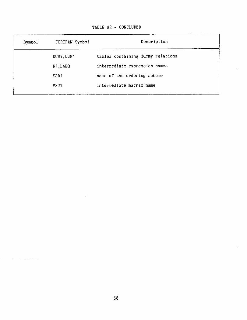
TABLE A3.- CONCLUDED

Symbol FORTRAN Symbol Description

DUMY,DUMI

RI,LAEQ

E2DI

VX2Y

tables containing dummy relations

intermediate expression names

name of the ordering scheme

intermediate matrix name

68

APPENDIX B

QUASI-STATIC APPROXIMATION

It is frequently possible to reduce the order of the system of equations

describing the rotorcraft dynamics by considering a quasi-static approximation for

certain degrees of freedom. Assume that the equations of motion have been reordered

so that the quasi-static variables (XO) appear last in the state vector.

(xl)x : (BI)

X0

The quasi-static approximation consists of neglecting the acceleration and

velocity terms of the quasi-static variables. Thus the equations of motion take the

form

V (B2)

The quasi-static variables are not Oescribed by differential equations but

rather by linear algebraic equations. The solution for (XO) then is simply

x0( 00)i 0, I= r_AolXl_ A1 _ AoO1X1! + BOy (B3)

Substituting for XO in the X I equation of motion gives then the reduced

order equations for the quasi-static approximation:

EA_I 10 00-1.01" 11 lO_AOO_-1.Ol- A0 (A 0 ) A2 ]X 1 + [A 1 - A0 A 1 ])(11 10- 00--1.01

I + [Ao AO- A0 (A0 ) ]X I

O0)-IBO= [B 1 - A_O(A 0 ]V (B4)

In the present analysis, the quasi-static approximation is applied to the

inflow dynamics and torsion degree of freedom of the blade.

69

REFERENCES

I. Proceedings of the 1977 MACSYMA User's Conference, Berkeley, Calif., July 1977,

NASA CP-2012.

. No,r, Ahmed K.; and Anderson, C. M.: Computerized Symbolic Manipulation in

Structural Mechanics-Progress and Potential. Computers and Structures,

vol. 10, 1979, pp. 95-118.

. Kiessling, F.: Computer Aided Derivation of Equations of Motion for Rotarywing

Aeroelastic Problems. ICAS-82-2.1.3, AIAA Aircraft Systems and Technology

Conference, Seattle, WA, Aug. 1982.

4. Arnold, R. M.: Rom, Manipulation of Algebraic Expressions. Comunications of

ACM, vol. 4, 1961, pp. 396-397.

5. Arnold, R. M.: Rom, Mechanized Algebraic Operations (MAO). Celestial Mechan-

ics, vol. I, 1970, pp. 301-319.

6. Broucke, R.; and Garthwaite, K.: A Programming System for Analytic Series

Expressions on a Computer. Celestial Mechanics, vol. I, 1969, pp. 271-284.

7. Jefferys, W. H.: A FORTRAN Based List Processor for Poisson Series. Celestial

Mechanics, vol. 2, no. 4, Nov. 1970, pp. 474-480.

. Broucke, R.: A FORTRAN-IV System for the Manipulation of Symbolic Poisson

Series with Application to Celestial Mechanics. Univ. of Texas, IASOM

TR 80-I, Jan. 1980.

9. Dasenbrock, R. R.: A FORTRAN Based Program for Computerized Algebraic Manipu-

lation. National Research Laboratories Report 8611, Sept. 1982.

10. Hale, A. L.; and Meirovitch, L.: A Special Purpose Symbolic Manipulation

Program for the Derivation of the Equations of Motion for Large Flexible

Structures. Presented at Conference on Dynamics and Control of Large Flexi-

ble Spacecraft, June 13-15, 1977, Ed. L. Meirovitch, Blaeksburg, Virginia.

11. Nagabhushanam, J.; Gaonkar, G. H.; and Reddy, T. S. R.: Automatic Generation

of Equations for Rotor-Body Systems with Dynamic Inflow for a Priori Order-

ing Schemes. 7th European Rotorcraft Forum, Paper No. 37, Sept. 8-11, 1981,

Garmish-Partenkirchen, Germany.

12. Ormiston, R. A.; and Hodges, D. H.: Linear Flap-Lag Dynamics of Hingeless

Rotor Blades in Hover. Journal of the American Helicopter Society, vol. 17,

no. 2, 1972, pp. 2-14.

70

13.

14.

15.

16.

17.

18.

19.

20.

21.

22.

23.

24.

Peters, D. A.: Flap-Lag Stability of Helicopter Rotor Blades in Forward

Flight. J. of the Am. Helicopter Soc., Oct. 1975, pp. 2-13.

Friedmann, P. P.; and Tong, P.: Nonlinear Flap-Lag Dynamics of Hingeless

Helicopter Blades in Hover and Forward Flight. J. of Sound and Vibration,

vol. 30, no. I, 1973, pp. 9-31.

Hodges, D. H.; and Ormiston, R. A.: Stability of Elastic Bending and Torsion

of Uniform Cantilever Rotor Blades in Hover with Variable Structural Cou-

pling. NASA TN D-8192, 1976.

Friedmann, P. P.; and Kottapalli, S. B. R.: Coupled Flap-Lag-Torsional Dynam-

ics of Hingeless Rotor Blades in Forward Flight. J. of the Am. Helicopter

Soc., vol. 27, no. 4, Oct. 1982, pp. 28-36.

Peters, D. A.; and Gaonkar, G. H.: Theoretical Flap-Lag Damping with Various

Inflow Models. J. of the Am. Helicopter Soc., vol. 25, no. 3, 1980,

pp. 29-36.

Gaonkar, G. H.; and Peters, D. A.: Use of Multiblade Coordinates for Helicop-

ter Flap-Lag Stability with Dynamic Inflow. J. of Aircraft, vol. 17, no. 2,

1980, pp. 112-118.

Gaonkar, G. H.; Sastry, V. V. S. S.; Reddy, T. S. R.; Nagabhushanam, J.; and

Peters, D. A.: The Use of Actuator-Disk Dynamic Inflow for Helicopter Flap-

Lag Stability. J. of the Am. Helicopter Soc., vol. 28, no. 3, 1983,

pp. 79-88.

Gaonkar, G. H.; Mitra, A. K.; Reddy, T. S. R.; and Peters, D. A.: Sensitivity

of Helicopter Aeromechanical Stability to Dynamic Inflow. Vertica, vol. 6,

no. I, 1982, pp. 59-67.

Johnson W.: Influence of Unsteady Aerodynamics on Hingeless Rotor Ground

Resonance. AIAA J. of Aircraft, vol. 19, no. 8, Aug. 1982, pp. 668-673.

Friedmann, P. P.: Formulation and Solution of Rotary Wing Aeroelastic Stabil-

ity and Response Problems. Paper no. 3.2, 8th European Rotorcraft Forum,

1982, Aix-En-Provence, France.

Hodges, D. H.; and Dowell, E. H.: Nonlinear Equations of Motion fop the Elas-

tic Bending and Torsion of Twisted Nonuniform Rotor Blades. NASA TN D-7818,

1974.

Kaza, K. R.; and Kvaternik, R. G.: Nonlinear Aeroelastic Equations for Com-

bined Flapwise Bending, Chordwise Bending, Torsion, and Extension of Twisted

Nonuniform Rotor Blades in Forward Flight. NASA TM 74059, 1977.

71

25.

26.

27.

28.

29.

30.

31.

Rosen, A.; and Friedmann, P. P.: Nonlinear Equations of Equilibrium for Elas-

tic Helicopter or Wind Turbine Blades Undergoing Moderate Deformation.

Report no. 7718, Univ. of California at Los Angles, Calif., Jan. 1977.

Johnson, Wayne: A Comprehensive Analytical Model of Rotorcraft Aerodynamics

and Dynamics, Part I: Analysis Development. NASA TM 81182, June 1980.

Brown, K. M.; and Dennis, J. E.: Derivative-Free Analogues of the Levenberg

Marquardt and Gauss Algorithms for Nonlinear Least Squares Approximations.

Numerische Mathematik, vol. 18, 1972, pp. 289-297.

Johnson, Wayne: Helicopter Theory. Princeton University Press, Princeton,

N.J., 1980.

Hodges, D. H.; Ormiston, R. A.; and Peters, D. A.: On the Nonlinear Deforma-

tion Geometry of Euler-Bernoulli Beams. NASA TP 1566, April 1980.

Peters, D. A.; and Ormiston, R. A.: The Effect of Second Order Blade Bending

on the Angle of Attack of Hingeless Rotor Blades. J. of the Am. Helicopter

Soc., vol. 18, no. 4, 1973, pp. 45-48.

Dugundji, John; and Wendell, J. H.: Some Analysis Methods for Rotating Systems

with Periodic Coefficients. AIAA J., vol. 21, no. 6, June 1983,

pp. 890-897.

72

TABLEI.- COMMANDSANDBRIEFDESCRIPTIONOFTHEIRFUNCTION

Command Function

Input commands

I. READEXPRESSION

2. READMATRIX

3. READTABLEFORSUBSTITUTION

4. READDIFFERENTIATIONTABLE

5. READGROUPANDORDEROFVARIABLES

6. READORDERINGSCHEME

7. READVARIABLESFORCOLLECTIONOFCOEFFICIENTS

8. READTAPE

Readsan expression name, numberof terms,and term details.

Readsa matrix name, size, and term detailsfor each element.

Readstable name, numberof relations, typeof table, and relation details.

Readsdifferentiation table name, numberofrelations, and relation details.

Readsgroup of each variable and its orderof magnitude.

Readsorder up to which variables of eachgroup can be retained.

Readsa group nameand variables for whichthe coefficients have to be collected.

Readsfrom a tape (disk), to separatesteady, and perturbed terms.

Algebraic manipulation commands

9. FORMEXPRESSION

10. FORMMATRIX

11. ADDMATRICES

12. CONSTANTMATRIX

13. MATRIXTO EXPRESSION

14. SUBSTITUTETABLEINTOEXPRESSION

Multiplies, adds, or subtracts two or moreexpressions.

Multiplies two matrices including transposemultiplication.

Addsor subtracts two compatible matrices.

Multiplies the matrix elements with a con-stant for expression having one term.

Converts matrix elements to expressionelements.

Substitutes a table of relations into anexpression.

73

TABLE I.- CONCLUDED

Command Function

Input commands - concluded

15. DIFFERENTIATE EXPRESSION Differentiates an expression with respect t(a variable.

Application commands

16. FORM LAGRANGIAN

17. INITIALIZE MULTIBLADE

18. PERFORM MULTIBLADE TRANSFORMATION

19. WRITE TAPE

20. NEGATE EXPRESSION

21. RESET COUNTER

22. END OF DATA

Program TRANS a

Uses Lagrangian formulation to generate

governing equations.

Generates multiblade functions.

Generates multiblade equations.

Writes on tape (disk) compatible with sym-

bolic program.

Gives the negative of an expression.

Erases unnecessary expressions.

Stops execution.

Codes the equations into FORTRAN subrou-tines.

aExecuted separately at present.

74

TABLE2.- FORTRANSYMBOLS

Originalvariable

R

U

UT

Up

UF

OF

V

FORTRAN

symbol

RAD

U

UD

UT

UP

UF

UFD

V

VD

Originalvariable

V !

vi

W

W !

X

B

n

FORTRAN

symbol

VS

LAMB

W

WS

WD

XCOR

THTA

PHI

OMEG

75

TABLE3.- TYPICALINPUTTOHESLANDOUTPUTTO CALCULATETANGENTIALANDNORMALVELOCITIES(UT ANDUp)

READMATRIX#LAFP0303O31.0

-0.5 VS VS

-0.5 WS WS

01

I.0 VS

01

I.0 WS02

-I.0 VS%EONE

-I.0 WS%ETWO

O3I.0 %ETRE-I.0 PHI THTA

- I.0 VS WS THTA

02

I.0 PHI

1.0 %EFUR THTA

O2

I.0 VS%ETWO

- I.0 WS%EONE

O3- I.0 %ETRE THTA-I .0 PHI

-I.0 VS WS

02

-I.0 PHI THTA

I.0 %EFURREAD MATRIX

# VEL0301

O3-I .0 UD

UFDOMEG V

VD

%XUUF OMEG

1.0

1.0

02

-I .0

-I .0

02

-I.0 OMEG RAD%LAMD

-I .0 WD

FORM MATRIX#LAFP# VEL#AVEL*E2DI

MATRIX EXPRESSION

02#AVEL

% UT0201% UP0301NEGATE EXPRESSION

% UT

76

TABLE 3.- CONCLUDED

NEGATE EXPRESSION

% UP

Note: %EONE, %ETWO, etc., are expressionsread earlier in the program.

Output of UT

I 1.000* VS*OMEG* V*2 1.000* VD*

3 1.000*XCOR*OMEG*4 1.000" U*OMEG*

5 -1.OO0" UF*OMEG*

6 -0.500* VS* VS* VD*

7 -0.500* VS* VS*XCOR*OMEG*8 -0.500* PHI* PHI* VD*

9 -0.500* PHI* PHI*XCOR*OMEG*10 -1.OOO* PHI*THTA* VD*

11 -1.O00* PHI*THTA*XCOR*OMEG*12 1.000" PHI*LAMB*OMEG* RAD*

13 1.0OO* PHI* WD*

14 1.000*THTA*LAMB*OMEG* RAD*

15 I.OOO*THTA* WD*

77

INPUT BASIC RELATIONS

11 SYMBOLIC DERIVATION OFGOVERNING EQUATIONS

!2 IDENTIFY ELEMENTS OF EACH

EQUATION AND INCORPORATEINTO FORTRAN SUBROUTINES

I

3 INPUT NUMERICAL DATACALCULATE STABI LITY

AND RESPONSE

(a) Flow chart.

Figure I.- Aeroelastic analyses.

78

INDIVIDUAL EXPRESSION INDIVIDUAL RELATION

RESOLVED

NUMERICAL

COEFFICIENT

INTO

NUMBERPATTERN

EXPRESSION ARRAY

RESOLVED

NUMERICAL

COEFFICENT

INTO

NUMBER

PATTE RN

TABLE ARRAY

COEFFICIENT PATTERN

STORAGE STORAGESTAC K STAC K

r

(b) Definition and storing of expressions and relations.

Figure I.- Concluded.

79

AXIS OF 8OJATION

FiEure 2.- RotOr blade coordinate s_stemS and deflections

ANGLE OF QUASIS_EADY

AEROFOIL _lONAND

LOADS

Figure 3.- inflow d_namics"

_0

-.06

HODGES AND DOWELL'S EQUATIONS, co¢ = 5.0

O'_ COMPUTER GENERATED EQUATIONS, _¢ = 5.0

[Z}--'-- HODGES AND DOWELL'S EQUATIONS, c_¢ = 2.5

O'm" COMPUTER GENERATED EQUATIONS,_¢=2.5

-.05

-.04

zO,.

:E<_a

-.03

.--I

,<LU

-.02

//

P

//!

-.01

I I I

0 .1 .2 ,3

STABLE

I

.4

Figure 4.- Comparison of lead-lag damping from two sets of equations for varying

pitch angle 8 for soft in-plane blade for two torsional frequencies, _v = 0.7,

mw = 1.15, R = 1.0, a = 0.1.

81

-.I0

-.02

0

Z

.18

.20

STABLEI

UNSTABLE

HODGES AND DOWELL'SEQUATIONS

COMPUTER GENERATED EQUATIONS

.22 l i0 .1 .2 .3 .4

Figure 5.- Comparison of lead-lag damping from two sets of equations for varying

pitch angle e for stiff in-plane blade for two torsional frequencies, _v = 1.5,

_w = 1.15, R = 1.0, a = 0.1.

82

-.015

-.014

-.013

-.012

-.011

-.010

zE -.009

<a

-.008<.J

6-.oo7<UJ-1

-.006

-.005

-.004

-.003

-.002

-.001

--O-- RIGID BLADE, R = 1.0

------ ELASTIC BLADE,(AERO-STIFFNESS TERMS ZERO)

-LASTICBLADE

STABLE

I I I

.1 .2 .38

Figure 6.- Lead-lag mode damping versus pitch angle 8, from flap-lag analysis for a

rigid blade model and an elastic blade model for a soft in-plane blade, _v = 0.7,

Uw = 1.15, R = 1.0, a = 0.05, Cdo = 0.01.

83

--O-- RIGID BLADE, R = 1.0

ELASTIC BLADE,(AERO-STIFFNESS TERMS ZERO)

ELASTIC BLADE

STABLE

RIGID BLADE, UNSTABLER=0

100 .1 .2 .3

Figure 7.- Lead-lag mode damping versus pitch angle e, from flap-lag analysis for a

rigid blade model and an elastic blade model for a stiff in-plane blade,

= 1.5, _w = 1.15, R = 1.0, o = 0.05, Cdo = 0.01._V

84

-3O

-28

-26

RIGID BLADE- h

DYNAMIC IN F LOW'-_

ELASTIC BLADE-DYNAMIC INF

RIGID BLADE-NO

DYNAMIC

ELASTIC BLADE-DYNAM IC IN FLOW

(AERO-STI FFNESS ZERO)

ELASTIC BLADE-NO

DYNAMIC INFLOW

STABLEI I I

0 .1 .2 .3 .4

Figure 8.- Lead-lag regressing mode damping with dynamic inflow versus pitch angle

e, from rigid blade model and elastic blade model for a soft in-plane blade,

uv : 0.7, _w : 1.15, R : 1.0, _ : 0.05.

85

-,10

/

AIIIt

I II l

l

------ WITH DYNAMIC INFLOW

WITHOUT DYNAMIC INFLOW

FLAP-LAG

STABLE

U NSTAB LE I

= 5.0

_¢ = 3.0

Figure 9.- The effect of torsion frequency and dynamic inflow on lead-lag regressing

mode damping versus lead-lag frequency, e = 0.3 rad, R = 0.0, mw = 1.15, a = 0.1.

86

-.20WITH DYNAMIC INFLOW

WITHOUT DYNAMIC INFLOW

Z -.15a.=E

Ill_3O:E

Z

-.10u.I

._1

_ -.05...I

//

//

//

// co¢ = 3.0

/

/ / \ \\/ / \

\\ co¢ = 5.0

STABLE

0. 5 i i ,1.0 1.5 2.0

coV

Figure I0.- The effect of torsion frequency and dynamic inflow on lead-lag regress-

ing mode damping versus lead-lag frequency, e = 0.3 tad, R = 1.0, =w = 1.15,o :0.I.

87

-.20WITH DYNAMIC INFLOW

WITHOUT DYNAMIC INFLOW

-.15

ZE.=E

DILlo -.10O

r,.9z

u.Ie¢-

i!1

ee -.05

..I

0

.05

R= 1.0

STABLE

UNSTABLE R = 0.4

R--0

l I

1.5 2.0

Figure 11.- The effect of elastic coupling and dynamic inflow on lead-lag regressing

mode damping versus lead-lag frequency, B = 0.3 tad, ,,,¢= 5.0, mw = 1.15,a : 0.1,

88

-.10

Za.

,,_-.05

LIJ

O=E

z

u.I

ee 0

=J

w.J

.05

------ WITH DYNAMIC INFLOW

WITHOUT DYNAMIC INFLOW

AP-LAG

"" 'Q" _ STABLE =

UNSTABLE '

I I i I I I I I

0 .I ,2 .3 .4 .5 .6 ,7 .8 .9 1.0R

Figure 12.- The effect of torsion frequency and dynamic inflow on lead-lag regress-

ing mode damping versus elastic coupling, e = 0.3 rad, _v = 1.4, _w = 1.15,o: 0.1.

89

-.4

Z

_-.3

_-.2

UJnr

n-

.Ju.

------ WITH DYNAMIC INFLOW

WITHOUT DYNAMIC INFLOW

_ FLAP-LAG

_._ _ _ _¢=5.0

.... _._ _ _¢ = 3.0_ "_=-.,--.,.=_._. _

FLAP-LAG"" _ _¢ = 5.0

_¢ = 3.0

I I I I I I |

•1 .2 .3 .4 .5 .6 .7R

STABLE

I I !

.8 .9 1.0

Figure 13.- The effect of torsion frequency and dynamic inflow on flap regressing

mode damping versus elastic coupling, e = 0.3 rad, _v = 1.4, _w = 1.15, a = 0.1.

9O

-.10

------ WITH DYNAMIC INFLOW

WITHOUT DYNAMIC INFLOW

1"-]_ QUASISTATIC INFLOW

_ u = vi-'_EQ. 12

O-- n u = vi'--_EQ. 12, QUASISTATIC INFLOW

STABLE

UNSTABLE

Figure 14.- Dynamic inflow modeling effects on lead-lag regressing mode damping

versus elastic coupling, e = 0.3 rad, _¢ = 5.0, _v = 1.4, mw = 1.15, o = 0.1.

91

-.10

-.05

7

iI

.050

----_ WITH DYNAMIC INFLOW

WITHOUT DYNAMIC INFLOW

O FLAP-LAG-TORSION

• QUASITORSION

f'l QUASITORSION-QUASISTATIC INFLOW

._._ UNSTABLEe,_" _._'J'_"-' STABLE I

1 I I I I I I I I I

.1 .2 .3 .4 .5 .6 .7 .8 .9 1.0

R

Figure 15.- Lead-lag regressing mode damping from flap-lag-torsion and quasi-static

torsion model with and without dynamic inflow versus elastic coupling parameter,

u¢ = 5.0, _w = 1.15, Uv = 1.4, e = 0. I, 0 = 0.3 rad.

92

-.10

O

D

----- WITH DYNAMIC INFLOW

WITHOUT DYNAMIC INFLOW

ELASTIC BLADE-QUASI TORSION

RIGID BLADE WITH PITCH-FLAP

AND PITCH-LAG COUPLINGS

STABLE

0 UNSTABLE i

I I I I I I 1 1 [ I

.1 .2 .3 .4 .5 .6 .7 .8 .9 1.0R

Figure 16.- Lead-lag regressing mode damping from a quasi-static torsion model and a

rigid blade flap-lag model with kinematic pitch-flap and pitch-lag couplings,

e = 0.3 tad, uv = 1.4, _w = 1.15, _¢ = 5.0.

93

Z

X_R = Vsin o_+ V i

SIDE VIEW

_ R

R cos ¢

R sin ¢

X

TOP VIEW

Y

Figure 17.- Aerodynamic velocity components in forward flight.

94

"_. -.016I,--ZuJz -.014OnXI.U¢..) -.012I--O3

-.OLOI-

< -.008rv"

-1-o -.006I.U"r

-.004LL0I..-_: -.002<a=J

"' 0

FLAP-LAG-TORSION TRIM

FLAP TRIM

1ST LEAD-LAG MODE

2ND LEAD-LAG MODE

.05 .10 .15 .20 .25 .30ADVANCE RATIO,

?

STABLE

.35 .40

Figure 18.- The effect of number of degrees of freedom used in trim analysis on

lead-lag damping versus advance ratio, soft in-plane, mv = 0.7, uw = 1.15,

uS = 3.0, o = 0.1, R = 1.0, propulsive trim.

95

-.06

i o FLAP-LAG-TORSION TRIM

• FLAP TRIM

-- 1STLEAD-LAGMODE / 1_, -- .

2,,X, -.04

tj

=<-.02

t-

ont-

,_1

<{iiin"

.02

UNSTABLE l

I . 1 |A | I

0 .05 .10 .35 .40 .45I J t I

.15 .20 .25 .30ADVANCE RATIO,

Figure 19.- The effect of number of degrees of freedom used in trim analysis on

lead-lag damping versus advance ratio, stiff in-plane, mv = 1.4, _w = 1.15,

_ = 3.0, o = 0.1, R = 1.0-, propulsive trim.

96

_,' -.016

Zua -.014Z0

X -.012LU

I'-O3

OCLUF-t.)<_ -.008

-1--.006

LLI"1"t--u. -.0040I-0:,_ -.002o.,_1

LUn.- 0

NUMBER OF MODES

o 2 FLAP, 2 LAG, 2 TORSION

A 2 FLAP, 2 LAG, 1 TORSION

c_ 2 FLAP, 2 LAG

1 TORSIONMODE

2 TORSIONMODES

FLAP-LAG

, 1,5n, , _ i.05 .10 . .20 .2 .30ADVANCE RATIO,/_

STABL EI I

.35 .40

Figure 20.- Lead-lag mode damping versus advance ratio for a flap-lag-torsion model

and a flap-lag model, soft in-plane, _v = 0.7, _w = I.15, _ = 3.0, a = 0.I,R = 1.0.

9T

NUMBER OF MODES

o 2 FLAP, 2 LAG, 2 TORSION

•", 2 FLAP, 2 LAG, 1 TORSION

o 2 FLAP, 2 LAG

1 TORSION

MODE

FLAP-LAG

2 TORSION

MODES

STABLE

l I 1 I I L ! I

.05 .10 .15 .20 .25 .30 .35 .40

ADVANCE RATIO, tJ

Figure 21.- Lead-lag mode damping versus advance ratio for a flap-lag-torsion model

and a flap-lag model, soft in-plane, _v = 0.7, uw = 1.15, ,,,_= 3.0, a = 0.I,R = 0.0.

98

-.06v

ZuJ

zOD.× -.04LU

I-

t,Y-LUI-(,.)< -.02

<'I-

LU-r"I.--It

O 0l.--re"<(3,.

..-I

<LUCE

NUMBER OF MODES

o 2 FLAP, 2 LAG, 2 TORSION

_ 2FLAP, 2LAG, 1TORSION /

o 2FLAP, 2LAG _ i t

1 TORSION

2 TORSION )_

i !MODE FLAP-LAG

STABLEI I I I t t I :

UNSTABLE

.02 ' ' ..... ' '0 .05 .10 .15 .20 .25 .30 .35 .40 .45

ADVANCE RATIO,/1

Figure 22.- Lead-lag mode damping versus advance ratio for a flap-lag-torsion model

and a slap-lag model, stiff in-plane, wv = 1.4, mw= 1.15, w@ = 3.0, o = 0.1,R = 1.0.

99

"_ -.02

zLLIZOa..XLUC.)i- 0

trLMI'--C.)

rr<"I"

,,, .02"1-I-U=

OI-.-rr<a..._1< .04LU

NUMBER OF MODES

o 2 FLAP, 2 LAG, 2 TORSION

A 2 FLAP, 2 LAG, 1 TORSION

[] 2 FLAP, 2 LAG

------ 2ND LEAD-LAG MODE, FLAP-LAG-TORSION

(2 MODES EACH)

FLAP_LAG, ,........ STABLE

__ _ ...,.,,_ _ ,.-"" -, , , , _ , ' -- --..J.' I

UNSTABLE

2 TORSION MODES

___ I I I I ] t I I

0 .05 .10 .15 .20 .25 .30 .35 .40ADVANCE RATIO,/1

Figure 23.- Lead-lag mode damping versus advance ratio for a flap-lag-torsion model

and a flap-lag model, stiff in-plane, _v = 1.4, _w = 1.15, _¢ = 3.0, a = 0.1,R : 0.0.

lOO

-.06

0

A

D

NUMBER OF MODES

2 FLAP, 2 LAG, 2 TORSION

2 FLAP, 2 LAG, 1 TORSION

2 FLAP, 2 LAG

--- 2ND LEAD-LAG MODE, FLAP-LAG-TORSION(2 MODES EACH)

1 TORSIONMODE

"2 TORSIONMODES

FLAP-LAG

STABLE

UNSTABLE

.02 ' ' ' ' ' J0 .2 .4 .6 .8 1.0

ELASTIC COUPLING PARAMETER, R

Figure 24.- Lead-lag mode damping versus elastic coupling for a flap-lag-torsion

model and flap-lag model, stiff in-plane, mv = 1.4, _w = 1.15, ,.,¢= 3.0, c = 0. I,: 0.25.

101

v .016

z,,, .014zO

X .012LU

I-_-- .010rt"LLII-

.008t_

"r".006

UJ

'-rI--u. .004OI.-nt-

.002

--I

ILl

t,.. 0

O

[]

FLAP-LAG-TORSION

FLAP-LAG

-- WITHOUT DYNAMIC INFLOW

WITH DYNAMIC INFLOW

STABLEI I L | I i ! •

.05 .10 .15 .20 .25 .30 .35 .40

ADVANCE RATIO,/.z

Figure 25.- The effect of torsion and dynamic inflow on lead-lag regressing mode

damping versus advance ratio, soft in-plane, "'v = 0.7, "'w = 1.15, uS = 3.0,o : 0.1, R : 1.0.

102

-.014z o FLAP-LAG-TORSION

zO -.012l't

XI,LI

_-- -.010I-t,./)n"w -.008I-¢.)<rr< -.006-r

LLI

-r -.004I-LLOI- -.002n,"<_a,.

..i

< 0ILl

rr

o FLAP-LAG

/'

I , , , _, , , SL.ABL=;T_

.05 .10 .15 .20 .25 .30 .35 .40

ADVANCE RATIO, ,u

Figure 26.- The effect of torsion and dynamic inflow on lead-lag regressing mode

damping versus advance ratio, soft in-plane, mv = 0.7, _w = 1.15, _¢ = 3.0,o : 0.1, R : 0.0.

103

-.06

ZLUZOa.X -.04LLI(3

I--

¢CLLII--(3

-.02

<.I-(.3U.l.1=I=.

14.

0 0i.=OC<a=_J

uJer-

o FLAP-LAG-TORSION

o FLAP-LAG

WITHOUT DYNAMIC INFLOW

. ------ WITH DYNAMIC INFLOW

/"'Q'\ _ /-_/

\\'Q- ._/'0/I I

STABLEI t I t t I t I

UNSTABLE

.02 ........ ' '0 .05 .10 .15 .20 .25 .30 .35 .40 .45

ADVANCE RATIO,/_

Figure 27.- The effect of torsion and dynamic inflow on lead-lag regressing mode

damping versus advance ratio, stiff in-plane, mv = 1.4, _w = 1.15, _¢ = 3.0,

o : 0.1, R : 1.0.

104

I.--" -.02zLLI

ZOQ,.

XLLI

I-(n 0n--LUI--L_<n"<-I-

"' .02-rI--M.

OI-n.-

(3..

,--I

<,,, .04r,"

o FLAP-LAG-TORSION

[] FLAP-LAG

WITHOUT DYNAMIC INFLOW

WITH DYNAMIC INFLOW z]......ET"*

ABLEI t t I I I I I

UNSTABLE

_i -'_ "o.

I | | l I | i |

0 .05 .10 .15 .20 .25 .30 .35 .40

ADVANCE RATIO, #

Figure 28.- The effect of torsion and dynamic inflow on lead-lag regressing mode

damping versus advance ratio, stiff in-plane, _v = 1.4, Uw = 1.15, _¢ = 3.0,o : 0.1, R = 0.0.

105

-.04

-.03v

ZLU

z0o. -.02XLU

I--CO

n"LU

I.-- -.01

<_m.-

<_"1"

LU'-rI-- 0IJL.

OI--mr

.,,,I

.01LUmr

.O20

FLAP-LAG-TORSION

FLAP-LAG

WITHOUT DYNAMIC INFLOW

------ WITH DYNAMIC INFLOW

//

/

//

/

STABLE

UNSTABLE

I I I I ! . I ._.l....._.._J

.2 .4 .6 .8 1.0

ELASTIC COUPLING PARAMETER, R

Figure 29.- The effect of torsion and dynamic inflow on lead-lag regressing mode

damping versus elastic coupling, stiff in-plane, my = 1.4, _w = 1.15, u$ = 3.0,

o = 0.1, _ : 0.25.

106

-.06

X -.04

f.)

o3,3_: -.02

"rf.)Ill"rI.-I,t=O 0I--n-

o.,.J

iii

-- WITHOUT DYNAMIC INFLOW

o REGRESSING MODE ._

v COLLECTIVE MODE l

a PROGRESSING MODE /

- WITH DYNAMIC INFLOW //- o REGRESSING MODE ,4"

j t i i i I STABLE,UNSTABLE

I

I j ,[ ,L_----_[ ..... ..1.__ = _ J

.02 0 .05 .10 .15 .20 .25 .30 .35 .40 .45

ADVANCE RATIO, #

Figure 30.- Comparison of constant coefficient approximation and Floquet analysis,

stiff in-plane, _v = 1.4, mw = 1.15, mS = 3.0, a = 0.1, R = 1.0.

107

,

1. Report No. 2. Government Acce_ion No.NASA TM-86750

4. Title and Subtitle

SYMBOLIC GENERATION OF ELASTIC ROTOR BLADE EQUATIONS USING

A FORTRAN PROCESSOR AND NUMERICAL STUDY ON DYNAMIC INFLOW

EFFECTS ON THE STABILITY OF HELICOPTER ROTORS

7. Author(s)

T. S. R. Reddy

9, Performing Organization Nameand Address

Ames Research Center

Moffett Field, CA 94035

12. Sponsoring A_ncy Name and Address

_ational Aeronautics and Space Administration

Washington, DC 20546

3. Recipient's Catalog No.

5. Report Date

June 1986

6. Performing Organization Code

8. Performing Organization Report No.

10. Work Unit No.

A-85227

11. Contract or Grant No.

13. Type of Report and Period Covered

Technical Memorandum

14. Sponsoring Agency Code

505-42-11

15 Supplementary Notes

Point of Contact: William Warmbrodt, Ames Research Center, MS 247-I, Moffett Field, CA 94035

(415) 694-5642 or FTS 464-5642

16. Abstract

The process of performing an automated aeroelastic stability analysis for an elastic-bladed

helicopter rotor is discussed. A symbolic manipulation program, written in FORTRAN, is used to ald

in the derivation of the governing equations of motion for the elastlc-bladed rotor. The blades

undergo coupled bending and torsional deformations. Two-dlmenslonal quasi-steady aerodynamics below

stall are used. Although reversed flow effects are neglected, unsteady effects, modeled as dynamic

inflow are included. Using a Lagrangian approach, the governing equations are derived in general-

ized coordinates using the symbolic program. The symbolic program generates the steady and per-

turbed equations and writes into subroutines to be called by numerical routines. The symbolic pro-

gram can operate both on expressions and on matrices. For the case of hovering flight, the blade

and dynamic inflow equations are converted to equations in a multiblade coordinate system by rear-

ranging the coefficients of the equations. For the case of forward flight, the multiblade equations

are obtained through the symbolic program. The final multiblade equations are capable of accom-

modating any number of elastic blade modes. The computer implementation of this procedure conslsts

of three stages: (I) the symbolic derivation of equations; (2) the coding of the equations into

subroutines; and (3) the numerical study after identifying mass, damping, and stiffness coefficients

for each equation. Damping results are presented in hover and in forward flight with, and without,

dynamic inflow effects for various rotor blade models, including rigid blade lag-flap, elastic flap-

lag, flap-lag-torsion, and quasl-static torsion. Results from dynamic inflow effects which are

obtained from a lift deficiency function for a quasl-static inflow model in hover are also

presented.

17. Key Words(Suggested by Author(s))

Symbolic processing

Helicopter

Rotary wing

Aeroelasticity

18. Distribution StatementUnlimited

m

19. SEurity Calif. (of this report) 20. Security Class_f. (of this page)

Unclassified Unclassified

Subject category - 05

21. No. of Pages 22. _ice"

*For sale by the National Technical Information Service, Springfield, Virginia 22161