Switching and Growth for Microbial Populations in Catastrophic Responsive Environments

Biophysical Journal Volume 98 April 2010 1099–1108 1099

Switching and Growth for Microbial Populations in CatastrophicResponsive Environments

Paolo Visco,† Rosalind J. Allen,†* Satya N. Majumdar,‡ and Martin R. Evans†

†SUPA, The University of Edinburgh, Edinburgh, United Kingdom; and ‡Laboratoire de Physique Theorique et Modeles Statistiques (UMR 8626du CNRS), Universite Paris-Sud, Orsay, France

ABSTRACT Phase variation, or stochastic switching between alternative states of gene expression, is common amongmicrobes, and may be important in coping with changing environments. We use a theoretical model to assess whether suchswitching is a good strategy for growth in environments with occasional catastrophic events. We find that switching can be advan-tageous, but only when the environment is responsive to the microbial population. In our model, microbes switch randomlybetween two phenotypic states, with different growth rates. The environment undergoes sudden catastrophes, the probabilityof which depends on the composition of the population. We derive a simple analytical result for the population growth rate.For a responsive environment, two alternative strategies emerge. In the no-switching strategy, the population maximizes itsinstantaneous growth rate, regardless of catastrophes. In the switching strategy, the microbial switching rate is tuned to minimizethe environmental response. Which of these strategies is most favorable depends on the parameters of the model. Previousstudies have shown that microbial switching can be favorable when the environment changes in an unresponsive fashionbetween several states. Here, we demonstrate an alternative role for phase variation in allowing microbes to maximize theirgrowth in catastrophic responsive environments.

INTRODUCTION

Microbial cells often exhibit reversible stochastic switching

between alternative phenotypic states, resulting in a heteroge-

neous population. This is known as phase variation (1–3).

A variety of molecular mechanisms can lead to phase varia-

tion, including DNA inversion, DNA methylation, and slip-

ped strand mispairing (1,2). These are generally two-state

systems without any underlying multistability (4,5); how-

ever, bistable genetic regulatory networks can also lead to

stochastic phenotypic switching (6–9). The biological func-

tion of phase variation remains unclear, but it has been sug-

gested that it can allow microbes to evade host immune

responses, or to access a wider range of host cell receptors

(3,10). Theoretical work has focused on phase variation

as a mechanism for coping with environmental changes.

According to this hypothesis, a fraction of the population

is maintained in a state which is currently less favorable,

but which acts as an insurance policy against future environ-

mental changes (11).

In this article, we present a theoretical model for switching

cells growing in an environment which occasionally makes

sudden attacks on the microbial population. Viewing the

situation from the perspective of the microbes, we term these

catastrophes. These catastrophes affect only one phenotypic

state. Importantly, the environment is responsive: the catas-

trophe rate depends on the microbial population. By solving

the model analytically, we find that there are two favored

tactics for microbial populations in environments with

Submitted August 10, 2009, and accepted for publication November 25,2009.

*Correspondence: [email protected]

Editor: Herbert Levine.

� 2010 by the Biophysical Society

0006-3495/10/04/1099/10 $2.00

a given feedback function: keep all the population in the

fast growing state, regardless of the environmental response,

or alternatively, use switching to maintain a population

balance that reduces the likelihood of an environmental

response. Which of these strategies is optimal depends on

the parameters of the model. In the absence of any feedback

between the population and environment, phase variation is

always unfavorable. However, as the environment becomes

more responsive, switching can be advantageous.

Previous theoretical studies have considered models in

which the environment flips randomly or periodically

between several different states, each favoring a particular

phenotype. The case of two environmental states and two

phenotypes has been well studied (12–17). This work has

shown that the total growth rate of the population can be

enhanced by phenotypic switching (compared to no switch-

ing) for some parameter regimes, and that the optimum

switching rate is tuned to the environmental flipping rate.

Several studies have also compared random switching to

a strategy where cells detect and respond to environmental

changes. Wolf et al. (17) used simulations to show that in

this case the advantage of random switching depends on the

accuracy of environmental sensing, whereas in a theoretical

study Kussell and Leibler (18) showed that the advantages of

random switching depend on the cost of environmental

sensing for a model with n phenotypic states and n differ-

ent environments. The predictions of the two-environment,

two-phenotypic state model have recently been verified

experimentally with a tunable genetic switch in the yeast

Saccharomyces cerevisiae (19).

Here, we consider a different scenario to the above-

mentioned body of work. Rather than considering multiple

doi: 10.1016/j.bpj.2009.11.049

mailto:[email protected]

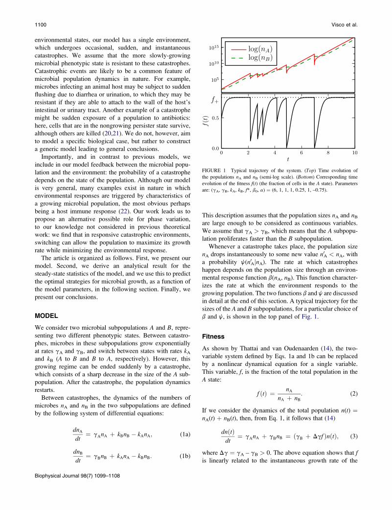
FIGURE 1 Typical trajectory of the system. (Top) Time evolution of

the populations nA and nB (semi-log scale). (Bottom) Corresponding time

evolution of the fitness f(t) (the fraction of cells in the A state). Parameters

are: (gA, gB, kA, kB, f*, b0, a) ¼ (6, 1, 1, 1, 0.25, 1, –0.75).

1100 Visco et al.

environmental states, our model has a single environment,

which undergoes occasional, sudden, and instantaneous

catastrophes. We assume that the more slowly-growing

microbial phenotypic state is resistant to these catastrophes.

Catastrophic events are likely to be a common feature of

microbial population dynamics in nature. For example,

microbes infecting an animal host may be subject to sudden

flushing due to diarrhea or urination, to which they may be

resistant if they are able to attach to the wall of the host’s

intestinal or urinary tract. Another example of a catastrophe

might be sudden exposure of a population to antibiotics:

here, cells that are in the nongrowing persister state survive,

although others are killed (20,21). We do not, however, aim

to model a specific biological case, but rather to construct

a generic model leading to general conclusions.

Importantly, and in contrast to previous models, we

include in our model feedback between the microbial popu-

lation and the environment: the probability of a catastrophe

depends on the state of the population. Although our model

is very general, many examples exist in nature in which

environmental responses are triggered by characteristics of

a growing microbial population, the most obvious perhaps

being a host immune response (22). Our work leads us to

propose an alternative possible role for phase variation,

to our knowledge not considered in previous theoretical

work: we find that in responsive catastrophic environments,

switching can allow the population to maximize its growth

rate while minimizing the environmental response.

The article is organized as follows. First, we present our

model. Second, we derive an analytical result for the

steady-state statistics of the model, and we use this to predict

the optimal strategies for microbial growth, as a function of

the model parameters, in the following section. Finally, we

present our conclusions.

MODEL

We consider two microbial subpopulations A and B, repre-

senting two different phenotypic states. Between catastro-

phes, microbes in these subpopulations grow exponentially

at rates gA and gB, and switch between states with rates kA

and kB (A to B and B to A, respectively). However, this

growing regime can be ended suddenly by a catastrophe,

which consists of a sharp decrease in the size of the A sub-

population. After the catastrophe, the population dynamics

restarts.

Between catastrophes, the dynamics of the numbers of

microbes nA and nB in the two subpopulations are defined

by the following system of differential equations:

dnA

dt¼ gAnA þ kBnB � kAnA; (1a)

dnB

dt¼ gBnB þ kAnA � kBnB: (1b)

Biophysical Journal 98(7) 1099–1108

This description assumes that the population sizes nA and nB

are large enough to be considered as continuous variables.

We assume that gA > gB, which means that the A subpopu-

lation proliferates faster than the B subpopulation.

Whenever a catastrophe takes place, the population size

nA drops instantaneously to some new value n0A < nA, with

a probability j(n0AjnA). The rate at which catastrophes

happen depends on the population size through an environ-

mental response function b(nA, nB). This function character-

izes the rate at which the environment responds to the

growing population. The two functions b and j are discussed

in detail at the end of this section. A typical trajectory for the

sizes of the A and B subpopulations, for a particular choice of

b and j, is shown in the top panel of Fig. 1.

Fitness

As shown by Thattai and van Oudenaarden (14), the two-

variable system defined by Eqs. 1a and 1b can be replaced

by a nonlinear dynamical equation for a single variable.

This variable, f, is the fraction of the total population in the

A state:

f ðtÞ ¼ nA

nA þ nB

: (2)

If we consider the dynamics of the total population n(t) ¼nA(t) þ nB(t), then, from Eq. 1, it follows that (14)

dnðtÞdt¼ gAnA þ gBnB ¼ ðgB þ Dgf ÞnðtÞ; (3)

where Dg ¼ gA – gB > 0. The above equation shows that fis linearly related to the instantaneous growth rate of the

FIGURE 2 The response function bl(f), plotted for different values of l,

with x ¼ 1 and f* ¼ 1/2.

Switching in Catastrophic Environments 1101

population (which is given by gB þ Dgf). For this reason,

and following Thattai and van Oudenaarden (14), we refer to

f as the population fitness.

The dynamical equation for the population fitness can be

determined from the Eqs. 1a and 1b, and corresponds to

df

dt¼ vðf Þ ¼ �Dgðf � fþ Þðf � f�Þ; (4)

where we define v(f) as the time evolution function for the

fitness, and f 5 are the two roots of the quadratic equation:

f 2 ��

1� kA þ kB

Dg

�f � kB

Dg¼ 0: (5)

One can check that the smaller root takes values f– < 0,

whereas the larger root takes values 0 < fþ % 1. Hence,

the population fitness increases toward a plateau value fþ,

until a catastrophe happens, upon which it is reset to a lower

value. A typical time trajectory for the population fitness

is plotted in the bottom panel of Fig. 1. The time evolution

of f is deterministic except at some specific time points

(catastrophes) where it undergoes random jumps. This model

can therefore be considered to be a Piecewise Deterministic

Markov Process (23,24).

Catastrophes

The catastrophes in our model have two characteristics: the

rate at which they happen and their strength (i.e., how many

microbes are killed). The rate at which catastrophes occur,

or their probability per unit time, is defined by a feedback

function b(f), which we take to depend only on the fitness

of the population and not on the absolute population size

(we shall return to this assumption later). The function b(f)characterizes the response of the environment to the growth

of the population. If b ¼ 0, there are no catastrophes and the

fitness will reach the plateau value fþ and stay there forever.

Nonzero constant values of b correspond to a nonresponsive

environment in which the catastrophes follow Poisson statis-

tics. We shall consider the case of a responsive environment

characterized by a response function b(f), which depends on

the population fitness. In particular, we consider a nonlinear

response function that has a sigmoid shape. Thus, the prob-

ability per unit time of a catastrophe is very low when the

population fitness is low, but increases significantly if the

fitness exceeds some threshold value. This scenario might

correspond to a detection threshold in the environment’s

sensitivity to population growth.

The precise environmental response function that we

consider is

blðf Þ ¼x

2

0B@1 þ f � f �ffiffiffiffiffiffiffiffiffiffiffiffiffiffiffiffiffiffiffiffiffiffiffiffiffiffiffiffiffi

l2 þ ðf � f �Þ2q

1CA: (6)

Although this function is defined over the whole range –N<f < N, the relevant interval for the fitness is 0 < f < 1.

Typical shapes for this function are shown in Fig. 2. The

parameter x is the asymptotic value of bl when f is large,

and we refer to x as the saturated catastrophe rate. As the

population fitness f increases, bl increases from 0 to x around

the threshold value f* at which bl ¼ x/2. Finally, the param-

eter l determines the sharpness of the threshold. For small

values of l, the function bl(f) approaches a step function

b0ðf Þ ¼ xQðf � f �Þ: (7)

As l increases, the function broadens and becomes linear

over a range of f near f*,

blxx

2

�1 þ ðf � f �Þ

lþ O

�1

l2

��; (8)

while, when the parameter l becomes very large (l / N),

bl(f) becomes constant (independent of f) so that the catastro-

phes become a standard Poisson process with parameter x/2:

bNðf Þ ¼ x=2: (9)

We emphasize that we have chosen this particular sigmoid

function Eq. 6 as the l parameter allows a convenient tuning

of its shape and thus the degree of environmental responsive-

ness. However, our conclusions are not affected by the

particular choice of sigmoid function.

We now turn to the function describing the catastrophe

strength, j(n0AjnA). This is the probability that, given that nA

cells of type A are present before the catastrophe, n0A will

remain after the catastrophe. To retain our description of the

model in terms of the population fitness, we shall consider

that j only depends on n0A through the ratio n0A/nA. Then

the normalization of j implies that

j�n0

A

��nA

�¼ 1

nA

F�n0

A=nA

�; (10)

whereR 1

0dx FðxÞ ¼ 1:


1102 Visco et al.

When a catastrophe occurs, the population size is reduced by

a random factor sampled from the distribution F (i.e., the

new size n0A ¼ nA � u, where nA is the size before the catas-

trophe, and u is a random number (0 % u < 1) sampled from

the distribution F ). This allows us to associate to each jump

nA / n0A a fitness jump f / f 0, where f 0 ¼ n0A/(n0A þ nB).

The size of these jumps will be distributed according to

m�

f0 ��f ¼ Q

�f � f

0F

f0 ð1� f Þ

f�1� f 0

�!

1� f�1� f 0

�2f: (11)

Equation 11 can be obtained by rewriting Eq. 10 for

j(n0AjnA) as a function of f and f 0, and including the

Jacobian of the transformation.

In this article, we shall consider the simple case where

FðxÞ ¼ ðaþ 1Þxa, with a > –1. The explicit expression

for j(n0jn) thus reads

j�n0 ��n� ¼ ða þ 1Þ

n

�n0

n

�a

; a > �1: (12)

This choice is made primarily to allow us to solve the model

analytically: the choice implies that m(f 0jf) factorizes (see

Eq. 13), which then allows the integral equation for the prob-

ability flux balance (Eq. 15) to be solved. Moreover, the

choice of a power law distribution for j(n0AjnA) is general

in that it allows for increasing, decreasing, or flat-functional

forms. The function j(n0AjnA) is plotted in Fig. 3 for various

values of a. For negative a-values, the distribution is biased

toward far-reaching catastrophes that reduce fitness signifi-

cantly. The case a ¼ 0 corresponds to jumps sampled from

a uniform distribution, whereas positive values give a distri-

bution biased toward weaker catastrophes. The parameter a

can therefore be used to tune the strength of the catastrophes

(although in this work we shall always consider negative

a-values, corresponding to strong catastrophes). We note

here that with our choice for FðxÞ the jump distribution can

be expressed as

m�f0 ��f � ¼ Q

�f � f

0� d

df 0m�f0�

mðf Þ ; (13)

FIGURE 3 The jump distribution j(n0AjnA), plotted for various values of a.


where mð0Þ ¼ 0;R

df0m�f0 jf�¼ 1; and with

mðf Þ ¼�

f

1� f

�1þ a

: (14)

STEADY-STATE STATISTICS

We now derive the steady-state probability distribution for

the population fitness, p(f). The distribution p(f) must satisfy

a condition of balance for the probability flux. This condition

reads

vðf Þpðf Þ ¼Z fþ

f

df0Z f

0

df 00b�f0�

p�f0�

m�f 00��f 0�: (15)

The left-hand side of the above equation corresponds to the

deterministic probability flux due to population growth as

defined in Eq. 4. (Note that f(t) increases in time as the pop-

ulation grows, as shown in Fig. 1.) The right-hand side

describes the probability flux arising from catastrophes. In

this model, catastrophes always reduce the population fitness.

The probability flux due to catastrophes therefore contains

contributions from all possible jumps that start at some f 0 >f and end at some f 00 < f. These contributions must be

weighted by b(f 0)p(f 0): the probability of having fitness f 0

and undergoing a catastrophe. This balance between the

fluxes due to growth and catastrophes is illustrated schemat-

ically in Fig. 4.

Inserting Eq. 13 for m(f 0jf) into Eq. 15, the zero flux condi-

tion becomes

vðf Þpðf Þ ¼Z fþ

f

df0b�f0�

p�f0�mðf Þ

m�f 0�: (16)

We now divide the above equation by m(f) and take the first

derivative with respect to f. This yields, in terms of the

function G ¼ vp/m,

dG

df¼ �bG

v: (17)

The above differential equation is then easily solved for G.

The result for p(f), using Eq. 14 for m(f), is finally

FIGURE 4 Illustration of the flux balance condition. The positive proba-

bility flux due to population growth must be balanced by the negative flux

due to catastrophes.

FIGURE 5 (Top panels) Examples of steady-state fitness

distribution p(f) for parameter values Dg ¼ 0.1 (left) and

100 (right); other parameters are l ¼ 0, kB ¼ 0.5, x ¼ 1,

a ¼ –0.99, and f* ¼ 0.75. In each plot, the solid line corre-

sponds to a value of kA ¼ 0 (no switching), whereas the

dashed plot is for kA ¼ kA* (switching rate given by

Eq. 19). (Bottom panels) Examples of fitness trajectories

corresponding to the parameter values of the top panel.


pðf Þ ¼ C

vðf Þ

�f

1� f

�1þa

exp

��Z

dfbðf Þvðf Þ

�; (18)

where C is a normalization constant. Equation 18 is the

central result of this section and gives the steady-state fitness

distribution for arbitrary functions b(f) and v(f). The integral

in Eq. 18 can be performed analytically for the model defined

in the previous section. The result, which is rather cumber-

some, is given in the Appendix.

We present in Fig. 5 (top panels) some resulting shapes

for the probability distribution p(f) in the case l ¼ 0, corre-

sponding to a step function for the environmental response.

We consider two different values of Dg, in each case for

kA ¼ 0 (no switching) and a nonzero switching rate kA ¼kA* defined such that fþ ¼ f* (see the next section). In these

plots we see that singularities in p(f) can arise at f ¼ 0, f*, or

fþ, in different cases.

We consider first the solid lines corresponding to kA ¼ 0.

Cusps in p(f) at f ¼ fþ ¼ 1 and f ¼ 0 (as seen in the rightpanel) reflect a population that maximizes its fitness in

between severe catastrophes that reduce f from 1 to 0;

however, a cusp at f ¼ f* (as seen in the left panel) reflects

a population that suffers catastrophes soon after the fitness

has crossed the threshold f*. In particular, the kA ¼ 0 case

produces a cusp at f ¼ f* (due to the singular nature of the

step function b(f) at f*) for small Dg, and/or a divergence

at f ¼ fþ for large Dg. On the other hand, the dotted lines

(where kA ¼ kA* and fþ ¼ f*) produce a divergence in both

right and left panels. This reflects a population that spends

much of its time at a fitness just below the threshold.

Fig. 5 (bottom panels) plots trajectories of the fitness cor-

responding to the parameter values of Fig. 5. These trajecto-

ries reveal the interplay between two timescales: the time to

relax to the plateau value f* in the absence of catastrophes

and the typical time between catastrophes. The former

decreases with Dg and the latter is given by 1/x where x is

the plateau value of the response function b. A divergence

of p(f) at f ¼ fþ arises when the plateau value is typically

reached before a catastrophe occurs.

OPTIMAL STRATEGIES: TO SWITCHOR NOT TO SWITCH?

The key question to be addressed in this work is whether

random switching is advantageous to the microbial popula-

tion in our model. To answer this question, we take advan-

tage of the analytical solution Eq. 18 to investigate how

the time-averaged population fitness depends on the rate

kA of switching from the fast-growing state A to the slow-

growing state B. We are particularly interested in the effect

of the parameter l, which controls the sharpness of the envi-

ronment’s response to the population.

In Fig. 6 we plot the average population fitness against kA

for several values of l. For a nonresponsive environment

(i.e., in the limit of large l, where the catastrophe rate takes

the constant nonzero value x/2 (See Eq. 9)), the population

fitness has only one (boundary) maximum for switching

rate kA / 0. This means that the optimal rate of population

growth is achieved when the bacteria do not switch away

from the fittest state A. It should be noted that we consider


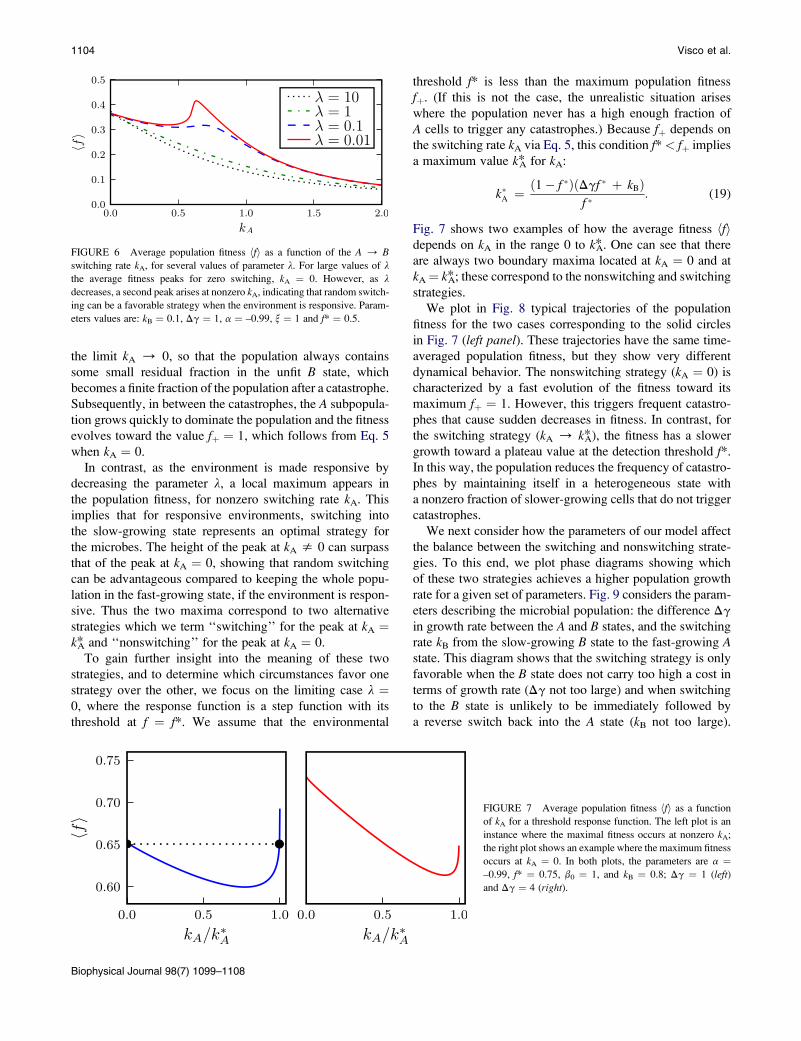
FIGURE 6 Average population fitness hfi as a function of the A / B

switching rate kA, for several values of parameter l. For large values of l

the average fitness peaks for zero switching, kA ¼ 0. However, as l

decreases, a second peak arises at nonzero kA, indicating that random switch-

ing can be a favorable strategy when the environment is responsive. Param-

eters values are: kB ¼ 0.1, Dg ¼ 1, a ¼ –0.99, x ¼ 1 and f* ¼ 0.5.

1104 Visco et al.

the limit kA / 0, so that the population always contains

some small residual fraction in the unfit B state, which

becomes a finite fraction of the population after a catastrophe.

Subsequently, in between the catastrophes, the A subpopula-

tion grows quickly to dominate the population and the fitness

evolves toward the value fþ ¼ 1, which follows from Eq. 5

when kA ¼ 0.

In contrast, as the environment is made responsive by

decreasing the parameter l, a local maximum appears in

the population fitness, for nonzero switching rate kA. This

implies that for responsive environments, switching into

the slow-growing state represents an optimal strategy for

the microbes. The height of the peak at kA s 0 can surpass

that of the peak at kA ¼ 0, showing that random switching

can be advantageous compared to keeping the whole popu-

lation in the fast-growing state, if the environment is respon-

sive. Thus the two maxima correspond to two alternative

strategies which we term ‘‘switching’’ for the peak at kA ¼k*A and ‘‘nonswitching’’ for the peak at kA ¼ 0.

To gain further insight into the meaning of these two

strategies, and to determine which circumstances favor one

strategy over the other, we focus on the limiting case l ¼0, where the response function is a step function with its

threshold at f ¼ f*. We assume that the environmental


threshold f* is less than the maximum population fitness

fþ. (If this is not the case, the unrealistic situation arises

where the population never has a high enough fraction of

A cells to trigger any catastrophes.) Because fþ depends on

the switching rate kA via Eq. 5, this condition f*< fþ implies

a maximum value k*A for kA:

k�A ¼ð1� f �ÞðDgf � þ kBÞ

f �: (19)

Fig. 7 shows two examples of how the average fitness hfidepends on kA in the range 0 to k*A. One can see that there

are always two boundary maxima located at kA ¼ 0 and at

kA¼ k*A; these correspond to the nonswitching and switching

strategies.

We plot in Fig. 8 typical trajectories of the population

fitness for the two cases corresponding to the solid circles

in Fig. 7 (left panel). These trajectories have the same time-

averaged population fitness, but they show very different

dynamical behavior. The nonswitching strategy (kA ¼ 0) is

characterized by a fast evolution of the fitness toward its

maximum fþ ¼ 1. However, this triggers frequent catastro-

phes that cause sudden decreases in fitness. In contrast, for

the switching strategy (kA / k*A), the fitness has a slower

growth toward a plateau value at the detection threshold f*.

In this way, the population reduces the frequency of catastro-

phes by maintaining itself in a heterogeneous state with

a nonzero fraction of slower-growing cells that do not trigger

catastrophes.

We next consider how the parameters of our model affect

the balance between the switching and nonswitching strate-

gies. To this end, we plot phase diagrams showing which

of these two strategies achieves a higher population growth

rate for a given set of parameters. Fig. 9 considers the param-

eters describing the microbial population: the difference Dg

in growth rate between the A and B states, and the switching

rate kB from the slow-growing B state to the fast-growing Astate. This diagram shows that the switching strategy is only

favorable when the B state does not carry too high a cost in

terms of growth rate (Dg not too large) and when switching

to the B state is unlikely to be immediately followed by

a reverse switch back into the A state (kB not too large).

FIGURE 7 Average population fitness hfi as a function

of kA for a threshold response function. The left plot is an

instance where the maximal fitness occurs at nonzero kA;

the right plot shows an example where the maximum fitness

occurs at kA ¼ 0. In both plots, the parameters are a ¼–0.99, f* ¼ 0.75, b0 ¼ 1, and kB ¼ 0.8; Dg ¼ 1 (left)

and Dg ¼ 4 (right).

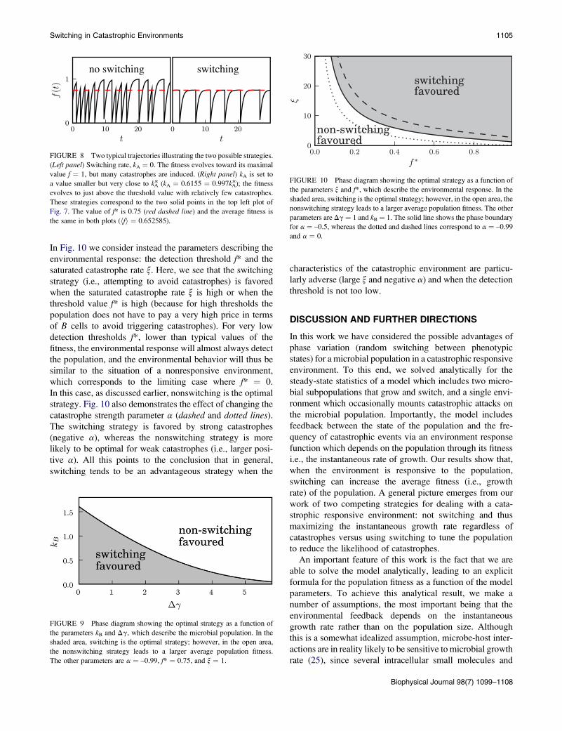
FIGURE 8 Two typical trajectories illustrating the two possible strategies.

(Left panel) Switching rate, kA ¼ 0. The fitness evolves toward its maximal

value f ¼ 1, but many catastrophes are induced. (Right panel) kA is set to

a value smaller but very close to k*A (kA ¼ 0.6155 ¼ 0.997k*A); the fitness

evolves to just above the threshold value with relatively few catastrophes.

These strategies correspond to the two solid points in the top left plot of

Fig. 7. The value of f* is 0.75 (red dashed line) and the average fitness is

the same in both plots (hfi ¼ 0.652585).

FIGURE 10 Phase diagram showing the optimal strategy as a function of

the parameters x and f*, which describe the environmental response. In the

shaded area, switching is the optimal strategy; however, in the open area, the

nonswitching strategy leads to a larger average population fitness. The other

parameters are Dg ¼ 1 and kB ¼ 1. The solid line shows the phase boundary

for a ¼ –0.5, whereas the dotted and dashed lines correspond to a ¼ –0.99

and a ¼ 0.


In Fig. 10 we consider instead the parameters describing the

environmental response: the detection threshold f* and the

saturated catastrophe rate x. Here, we see that the switching

strategy (i.e., attempting to avoid catastrophes) is favored

when the saturated catastrophe rate x is high or when the

threshold value f* is high (because for high thresholds the

population does not have to pay a very high price in terms

of B cells to avoid triggering catastrophes). For very low

detection thresholds f*, lower than typical values of the

fitness, the environmental response will almost always detect

the population, and the environmental behavior will thus be

similar to the situation of a nonresponsive environment,

which corresponds to the limiting case where f* ¼ 0.

In this case, as discussed earlier, nonswitching is the optimal

strategy. Fig. 10 also demonstrates the effect of changing the

catastrophe strength parameter a (dashed and dotted lines).

The switching strategy is favored by strong catastrophes

(negative a), whereas the nonswitching strategy is more

likely to be optimal for weak catastrophes (i.e., larger posi-

tive a). All this points to the conclusion that in general,

switching tends to be an advantageous strategy when the

FIGURE 9 Phase diagram showing the optimal strategy as a function of

the parameters kB and Dg, which describe the microbial population. In the

shaded area, switching is the optimal strategy; however, in the open area,

the nonswitching strategy leads to a larger average population fitness.

The other parameters are a ¼ –0.99, f* ¼ 0.75, and x ¼ 1.

characteristics of the catastrophic environment are particu-

larly adverse (large x and negative a) and when the detection

threshold is not too low.

DISCUSSION AND FURTHER DIRECTIONS

In this work we have considered the possible advantages of

phase variation (random switching between phenotypic

states) for a microbial population in a catastrophic responsive

environment. To this end, we solved analytically for the

steady-state statistics of a model which includes two micro-

bial subpopulations that grow and switch, and a single envi-

ronment which occasionally mounts catastrophic attacks on

the microbial population. Importantly, the model includes

feedback between the state of the population and the fre-

quency of catastrophic events via an environment response

function which depends on the population through its fitness

i.e., the instantaneous rate of growth. Our results show that,

when the environment is responsive to the population,

switching can increase the average fitness (i.e., growth

rate) of the population. A general picture emerges from our

work of two competing strategies for dealing with a cata-

strophic responsive environment: not switching and thus

maximizing the instantaneous growth rate regardless of

catastrophes versus using switching to tune the population

to reduce the likelihood of catastrophes.

An important feature of this work is the fact that we are

able to solve the model analytically, leading to an explicit

formula for the population fitness as a function of the model

parameters. To achieve this analytical result, we make a

number of assumptions, the most important being that the

environmental feedback depends on the instantaneous

growth rate rather than on the population size. Although

this is a somewhat idealized assumption, microbe-host inter-

actions are in reality likely to be sensitive to microbial growth

rate (25), since several intracellular small molecules and


1106 Visco et al.

proteins, including ppGpp, cAMP, and H-NS, whose concen-

trations are growth-rate-dependent (26,27), have been shown

to regulate microbial virulence factors (28–30).

The main conclusion of our work is that phase variation

can provide a mechanism by which a microbial population

can tune its composition so as to minimize the likely environ-

mental response, thus increasing its average growth rate

(or average fitness). The model then provides an alternative

scenario for the role of phase variation to those proposed in

other theoretical studies, which we now take the opportunity

to review briefly.

Various works have considered models in which the envi-

ronment flips randomly or periodically between several

different states, each favoring a particular cell phenotype.

These models do not include feedback between the popula-

tion and the environmental flipping rate. For the case of

two environmental states and two cellular phenotypes,

Lachmann and Jablonka (12) considered a discrete time

model with a periodic environment, whereas Ishii et al.

(13) addressed a similar problem but explicitly looked for

the evolutionary stable state. Thattai and Van Oudenaarden

(14) also considered the two-environment, two-phenotype

case, using a continuous time model with Poissonian switch-

ing of the environment. A detailed analytical treatment of

this case was presented by Gander et al. (15) and a simulation

study was carried out by Ribeiro (16) with a more detailed

model of the phenotypic switching mechanism, and Wolf

et al. (17) simulated a model that also included environ-

mental sensing. These studies showed that the total growth

rate of the population can be enhanced by phenotypic switch-

ing (compared to no switching), for some parameter regimes,

and that the optimum switching rate is tuned to the environ-

mental flipping rate. A similar model, but aimed specifically

at the case of the persister phenotype, in which cells grow

very slowly but are resistant to antibiotics (20), was consid-

ered by Kussell et al. for a periodic environment (21). In this

model, the growth rate of the nonpersister phenotype is

negative (signifying population decrease) in the antibiotic

environment.

Several other studies have considered random switching

from a different context: as a means to avoid the need for

sensing and responding to environmental changes, in the

case that environmental sensing is inaccurate, faulty, or

expensive. In this context, Kussell and Leibler (18) consid-

ered theoretically a model with many environments and

many cellular states, where a cost is attached to sensing envi-

ronmental changes, whereas Wolf et al. (17) simulated

a two-state, two-environment model where sensing was

subject to a variety of possible defects. Both these studies

concluded that random switching can be a good strategy to

overcome disadvantages associated with environmental

sensing.

In a somewhat different approach, Wolf et al. (31) used

simulations to study a two-state, two-environment model in

which the growth rate of the A and B states is frequency-


dependent—i.e., a given microbial subpopulation grows

faster when its abundance is low. Such frequency-dependent

selection is well known to promote population heteroge-

neity; however, Wolf et al. did not find any advantages for

reversible switching as a means to generate this heteroge-

neity as opposed to terminal cellular differentiation. In

a sense, the model presented in this article also incorporates

frequency-dependent selection, because catastrophes are less

likely when the A subpopulation is small. However, in

contrast to Wolf et al., we find that reversible switching

does play an important role. If switching in our model

were not reversible, there would be no way for the fast-

growing A subpopulation to regenerate from the surviving

B cells after a catastrophe.

Although the majority of theoretical work in this area,

including that presented in this article, has focused on the

interplay between cellular switching and environmental

changes, this is not the only perspective from which the

role of phase variation can be viewed. For example, an alter-

native scenario, which does not require a changing environ-

ment, was recently presented by Ackermann et al.

(32). These authors showed that random switching into

a self-sacrificing phenotypic state can be evolutionarily

favored if the individuals in that state have, on average,

greater access to some beneficial resource. This idea raises

a number of interesting questions which we hope to pursue

in future research.

Finally we note that the theoretical framework developed

in this work, although applied here to the case of detrimental

and instantaneous catastrophes, could also be used to model

environmental changes more generally. For example, in the

symmetric two-state, two-environment model considered

by Thattai and van Oudenaarden (14) and others, the envi-

ronment flips randomly between two states and these flips

are accompanied by a change in fitness from f to 1 – f.This could be incorporated in our theoretical framework by

setting the b(f) to a constant value and the jump distribution

m(f j f 0) to

m�f0 �� f � ¼ d

�f0 � ð1� f Þ

�: (20)

However, such a choice of m(f j f0) would result in funda-

mentally different conclusions to those of this study, because

the fitness in the model of Thattai and van Oudenaarden (and

in other similar models) is not necessarily decreased when

the environment changes. In fact, if a large fraction of the

cells is in the slow-growing state before the environment

flips so that f< 1/2, then the environmental change will actu-

ally increase the fitness of the population. In contrast, in this

work, all catastrophes are detrimental and the advantage of

switching lies in avoiding the triggering of an environmental

response.

This study suggests a number of avenues for further work.

First, it would be useful to check the robustness of the results

to changes in the choice of catastrophe distributions. Here we

Zdf

bðf Þvðf Þ ¼

x

2DgDflog

8<:ðf � f�Þðfþ � f Þ

2Df ððf � � f Þðf � � f�Þ þ l2 þ gðf ; f �Þgðf�; f �ÞÞ

ðf � f�Þðf � � f�Þgðf�; f �Þ

�ðf ��f�Þgðf� ;f �Þ

�

2Df ððf � f �Þðfþ � f �Þ þ l2 þ gðf ; f �Þgðfþ ; f �ÞÞðfþ � f Þðfþ � f �Þgðfþ ; f �Þ

�ðfþ �f �Þgðfþ ;f �Þ

9=;;

(21)


have adopted the power law (Eq. 12) which allows the exact

solution of the model and generates a broad range of catas-

trophes sizes. Such a distribution could be justified in the

context of an antibiotic environment, as representing the

dose-response variability of antimicrobes (33) and variability

in the dosage. One could also explore other distributions

such as exponentially distributed catastrophes or those

centered about some particular catastrophe fraction f 0 ¼ afwith a < 1. It remains to be determined which choice is

most biologically relevant in different contexts.

Another point that deserves investigation in future work is

the relation between the choice of switching strategy and the

variability in the population fitness. For example in Fig. 5

one can see that the different strategies give very different

widths for the fitness distribution p(f). In this work we

defined the optimal strategy as that which gives the maximal

average growth of the population. However, it might also be

relevant to include fitness fluctuations in the criteria for opti-

mality.

It is also important to consider the case where the envi-

ronmental response depends on the absolute size of a partic-

ular subpopulation. Here, we expect that the population size

may reach a steady state governed by the balance between

growth and catastrophes. The total population size could

then be maximized either by maximizing the growth rate,

regardless of catastrophes, or by tuning the population com-

position to avoid triggering catastrophes. We thus expect

that the two strategies identified in this work will prove to

be relevant to a variety of models. Moreover, we note that

the distinction between models based on growth rate and

those based on population size may vanish for scenarios

with constant population size such as chemostat cultures

(34). Equally interesting are the prospects for including

spatial effects, such as adhesion to host surfaces, or transfer

between different environmental compartments, in the

model, and for generalizing the model to include many

different microbial states, in which case the same theoretical

framework could perhaps be used to describe genetic evolu-

tion of microbial populations in catastrophic responsive

environments.

APPENDIX: EXPLICIT FORM OF P(F)

Below we give the explicit form for the integral appearing

in Eq. 18 when b(f) is given by Eq. 6,

where

gða; bÞ ¼ffiffiffiffiffiffiffiffiffiffiffiffiffiffiffiffiffiffiffiffiffiffiffiffiffiffiða� bÞ2þ l2

q: (22)

From this result, the explicit expression for the fitness distri-

bution function p(f) can be easily derived.

The authors are grateful to David Gally and Otto Pulkkinen for useful

discussions.

R.J.A. was funded by the Royal Society. This work was supported by

the Engineering and Physical Sciences Research Council under grant No.

EP/E030173.

REFERENCES

1. van der Woude, M. W., and A. J. Baumler. 2004. Phase and antigenicvariation in bacteria. Clin. Microbiol. Rev. 17:581–611.

2. van der Woude, M. W. 2006. Re-examining the role and random natureof phase variation. FEMS Microbiol. Lett. 254:190–197.

3. Henderson, I. R., P. Owen, and J. P. Nataro. 1999. Molecularswitches—the ON and OFF of bacterial phase variation. Mol. Micro-biol. 33:919–932.

4. Visco, P., R. J. Allen, and M. R. Evans. 2008. Exact solution of a modelDNA-inversion genetic switch with orientational control. Phys. Rev.Lett. 101:118104.

5. Visco, P., R. J. Allen, and M. R. Evans. 2009. Statistical physics ofa model binary genetic switch with linear feedback. Phys. Rev. E Stat.Nonlin. Soft Matter Phys. 79:031923.

6. Ptashne, M. 1992. A Genetic Switch, Phage l and Higher Organisms,2nd Ed. Blackwell, Cambridge, New York.

7. Novick, A., and M. Weiner. 1957. Enzyme induction as an all-or-nonephenomenon. Proc. Natl. Acad. Sci. USA. 43:553–566.

8. Carrier, T. A., and J. D. Keasling. 1999. Investigating autocatalytic geneexpression systems through mechanistic modeling. J. Theor. Biol.201:25–36.

9. Warren, P. B., and P. R. ten Wolde. 2005. Chemical models of genetictoggle switches. J. Phys. Chem. B. 109:6812–6823.

10. Hallet, B. 2001. Playing Dr Jekyll and Mr Hyde: combined mechanismsof phase variation in bacteria. Curr. Opin. Microbiol. 4:570–581.

11. Seger, J., and H. Brockman. 1987. What is bet-hedging? In Oxford Surveysin Evolutionary Biology.. Oxford University Press, Cambridge, UK.

12. Lachmann, M., and E. Jablonka. 1996. The inheritance of phenotypes:an adaptation to fluctuating environments. J. Theor. Biol. 181:1–9.

13. Ishii, K., H. Matsuda, ., A. Sasaki. 1989. Evolutionarily stable mutationrate in a periodically changing environment. Genetics. 121:163–174.

14. Thattai, M., and A. van Oudenaarden. 2004. Stochastic gene expressionin fluctuating environments. Genetics. 167:523–530.

15. Gander, M. J., C. Mazza, and H. Rummler. 2007. Stochastic geneexpression in switching environments. J. Math. Biol. 55:259–294.

16. Ribeiro, A. S. 2008. Dynamics and evolution of stochastic bistable genenetworks with sensing in fluctuating environments. Phys. Rev. E Stat.Nonlin. Soft Matter Phys. 78:061902.


1108 Visco et al.

17. Wolf, D. M., V. V. Vazirani, and A. P. Arkin. 2005. Diversity in timesof adversity: probabilistic strategies in microbial survival games.J. Theor. Biol. 234:227–253.

18. Kussell, E., and S. Leibler. 2005. Phenotypic diversity, populationgrowth, and information in fluctuating environments. Science.309:2075–2078.

19. Acar, M., J. T. Mettetal, and A. van Oudenaarden. 2008. Stochasticswitching as a survival strategy in fluctuating environments. Nat. Genet.40:471–475.

20. Balaban, N. Q., J. Merrin, ., S. Leibler. 2004. Bacterial persistence asa phenotypic switch. Science. 305:1622–1625.

21. Kussell, E., R. Kishony, ., S. Leibler. 2005. Bacterial persistence:a model of survival in changing environments. Genetics. 169:1807–1814.

22. Mulvey, M. A. 2002. Adhesion and entry of uropathogenic Escherichiacoli. Cell. Microbiol. 4:257–271.

23. Davis, M. H. A. 1984. Piecewise-deterministic Markov processes:a general class of non-diffusion stochastic models. J. R. Stat. Soc. B.46:353–388.

24. Pulkkinen, O., and J. Berg. 2008. Dynamics of gene expression underfeedback. arXiv:0807.3521.

25. Johri, A. K., V. Patwardhan, and L. C. Paoletti. 2005. Growth rate andoxygen regulate the interactions of group B Streptococcus with polar-ized respiratory epithelial cells. Can. J. Microbiol. 51:283–286.


26. Ferenci, T. 2008. Bacterial physiology, regulation and mutational adap-

tation in a chemostat environment. Adv. Microb. Physiol. 53:169–229.

27. Schaechter, M., J. L. Ingraham, and F. C. Neidhardt. 2006. Microbes.

ASM Press, Washington, DC.

28. Pizarro-Cerda, J., and K. Tedin. 2004. The bacterial signal molecule,

ppGpp, regulates Salmonella virulence gene expression. Mol. Micro-

biol. 52:1827–1844.

29. Pesavento, C., and R. Hengge. 2009. Bacterial nucleotide-based second

messengers. Curr. Opin. Microbiol. 12:170–176.

30. Schroder, O., and R. Wagner. 2002. The bacterial regulatory protein

H-NS—a versatile modulator of nucleic acid structures. Biol. Chem.

383:945–960.

31. Wolf, D. M., V. V. Vazirani, and A. P. Arkin. 2005. A microbial modi-

fied prisoner’s dilemma game: how frequency-dependent selection can

lead to random phase variation. J. Theor. Biol. 234:255–262.

32. Ackermann, M., B. Stecher, ., M. Doebeli. 2008. Self-destructive

cooperation mediated by phenotypic noise. Nature. 454:987–990.

33. Nightingale, C. H., P. G. Ambrose, and G. L. Drusano. 2007. Antimi-

crobial Pharmacodynamics in Theory and Clinical Practice, 2nd Ed.

Informa Healthcare, New York.

34. Ingraham, J. L., O. Maaloe, and F. C. Neidhardt. 1983. Growth of the

Bacterial Cell. Sinauer Associates, Sunderland, MA.

Documents

Switching and Growth for Microbial Populations in Catastrophic Responsive Environments