SVM May 2007

SVM

May 2007

DOE-PI

Dianne P. O’Leary

c©2007

1

Speeding the Training of Support Vector Machines

and Solution of Quadratic Programs

Dianne P. O’Leary

Computer Science Dept. andInstitute for Advanced Computer Studies

University of Maryland

Jin Hyuk Jung

Computer Science Dept.

Andre Tits

Dept. of Electrical and Computer Engineering andInstitute for Systems Research

Work supported by the U.S. Department of Energy.

2

The Plan

• Introduction to SVMs

• Our algorithm

• Convergence results

• Examples

3

a d = +1 (yes)d = -1 (no)

What is an SVM?

SVM

4

SVM

wTa – >0?a d = +1 (yes)

d = -1 (no)

What’s inside the SVM?

5

a d = +1 (yes)d = -1 (no)

SVM wTa – >0?

How is an SVM “trained”?

w,

a1, d1…

am, dm

IPM forQuadratic Programming

wTa – >0?

SVM

6

The problem: training an SVM

Given: A set of sample data points ai, in sample space S, with labelsdi = ±1, i = 1, . . . , m.

Find: A hyperplane x : 〈w,x〉 − γ = 0, such that

sign(〈w,ai〉 − γ) = di,

or, ideally,di(〈w,ai〉 − γ) ≥ 1.

7

Which hyperplane is best?

We want to maximize the separation margin 1/‖w‖.

8

Generalization 1

We might map a more general separator to a hyperplane through sometransformation Φ:

For simplicity, we will assume that this mapping has already been done.

9

Generalization 2

If there is no separating hyperplane, we might want to balance maximizingthe separation margin with a penalty for misclassifying data by putting iton the wrong side of the hyperplane. This is the soft-margin SVM.

• We introduce slack variables y ≥ 0 and relax the constraintsdi(〈w,ai〉 − γ) ≥ 1 to

di(〈w,ai〉 − γ) ≥ 1 − yi.

• Instead of minimizing ‖w‖, we solve

minw,γ,y

1

2‖w‖2

2+ τeTy

for some τ > 0, subject to the relaxed constraints.

10

Jargon

Classifier 〈w,x〉 − γ = 0: black lineBoundary hyperplanes: dashed lines2 × separation margin: length of arrowSupport vectors: On-Boundary (yellow) and Off-Boundary (green)Non-SV: blue

Key point: The classifier is the same, regardlessof the presence or absence of the blue points.

11

Summary

• The process of determining w and γ is called training the machine.

• After training, given a new data point x, we simply calculatesign(〈w,x〉 − γ) to classify it as in either the positive or negative group.

• This process is thought of as a machine – called the support vectormachine (SVM).

• We will see that training the machine involves solving a convexquadratic programming problem whose number of variables is thedimension n of the sample space and whose number of constraints isthe number m of sample points – typically very large.

12

Primal and dual

Primal problem:

minw,γ,y1

2‖w‖2

2+ τeTy

s.t. D(Aw − eγ) + y ≥ e,

y ≥ 0,

Dual problem:

maxv −1

2vTHv + eTv

s.t. eTDv = 0,

0 ≤ v ≤ τe,

where H = DAATD ∈ Rm×m is a symmetric and positive semidefinite

matrix withhij = didj〈ai, aj〉.

13

Support vectors

Support vectors (SVs) are the patterns that contribute to defining theclassifier.

They are associated with nonzero vi.

vi si yi

Support vector (0, τ ] 0 [0,∞)On-Boundary SV (0, τ ) 0 0Off-Boundary SV τ 0 (0,∞)

Nonsupport vector 0 (0,∞) 0

• vi: dual variable (Lagrange multiplier for relaxed constraints).

• si: slack variable for primal inequality constraints.

• yi: slack variable in relaxed constraints.

14

Solving the SVM problem

Apply standard optimization machinery:

• Write down the optimality conditions for the primal/dual formulationusing the Lagrange multipliers. This is a system of nonlinear equations.

• Apply a (Mehotra-style predictor-corrector) interior point method (IPM)to solve the nonlinear equations by tracing out a path from a givenstarting point to the solution.

15

The optimality conditions

w − ATDv = 0,

dTv = 0

τe − v − u = 0,

DAw − γd + y − e − s = 0,

Sv = σµe,

Yu = σµe,

s,u, v, y ≥ 0.

for σ = 0.

Interior point method (IPM): Let 0 < σ < 1 be a centering parameter andlet

µ =sTv + yTu

2m.

Follow the path traced as µ → 0, σ = 1.

16

A step of the IPM

At each step of the IPM, the next point on the path is computed using avariant of Newton’s method applied to the system of equations.

This gives a linear system for the search direction:

I −ATD

dT

−I −I

DA −I I −d

S V

Y U

∆w

∆v

∆u

∆s

∆y

∆γ

=

−(w − ATDv)

−dTv

−(τe − v − u)−(DAw − γd + y − e − s)

−Sv

−Yu

By block elimination, we can reduce this system to

M ∆w = some vector

(sometimes called the normal equations).

17

The matrix for the normal equations

M ∆w = some vector

M = I + ATDΩ−1DA − ddT

dTΩ−1d.

Here, D and Ω are diagonal, d = ATDΩ−1d, and

ω−1

i =viui

sivi + yiui.

Given ∆w, we can easily find the other components of the direction.

18

Two variants of the IPM algorithm

• In affine scaling algorithms, σ = 0. Newton’s method then aims to solvethe optimality conditions for the optimization problem.

Disadvantage: We might not be in the domain of fast convergence forNewton.

• In predictor-corrector algorithms, the affine scaling step is used tocompute a corrector step with σ > 0. This step draws us back towardthe path.

Advantage: Superlinear convergence can be proved.

19

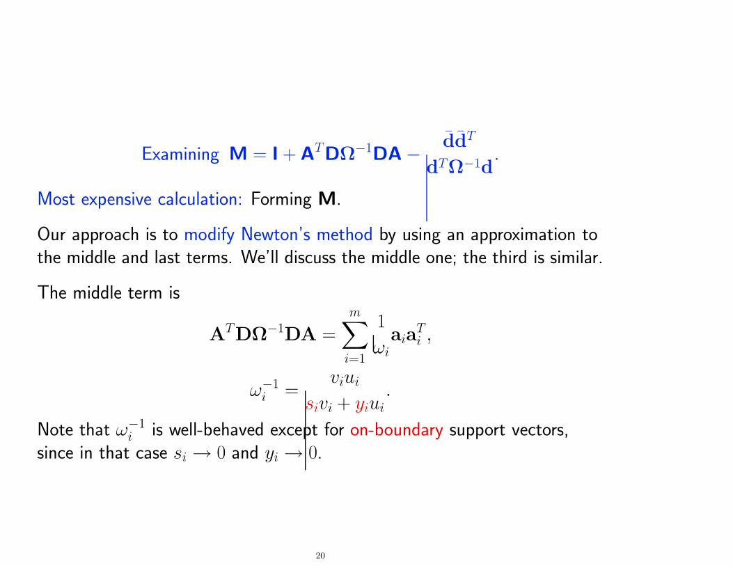
Examining M = I + ATDΩ−1DA − ddT

dTΩ−1d.

Most expensive calculation: Forming M.

Our approach is to modify Newton’s method by using an approximation tothe middle and last terms. We’ll discuss the middle one; the third is similar.

The middle term is

ATDΩ−1DA =m

∑

i=1

1

ωiaia

Ti ,

ω−1

i =viui

sivi + yiui.

Note that ω−1

i is well-behaved except for on-boundary support vectors,since in that case si → 0 and yi → 0.

20

Our idea:

We only include terms corresponding to constraints we hypothesize areactive at the optimal solution.

We could

• ignore the value of di.

• balance the number of positive and negative patterns included.

The number of terms is constrained to be

• at least qL, which is the minimum of n and the number of ω−1 valuesgreater than θ

√µ, for some parameter θ.

• at most qU , which is a fixed fraction of m.

21

Some related work

• Use of approximations to M in LP-IPMs dates back to Karmarkar(1984), and adaptive inclusion of terms was studied, for example, byWang and O’Leary (2000).

• Osuna, Freund, and Girosi (1997) proposed solving a sequence of CQPs,building up patterns as new candidates for support vectors are identified.

• Joachims (1998) and Platt(1999) used variants related to Osuna et al.

• Ferris and Munson (2002) focused on efficient solution of normalequations.

• Gertz and Griffin (2005) used preconditioned cg, with a preconditionerbased on neglecting terms in M.

22

Convergence analysis for Predictor-Corrector Algorithm

All of our convergence results are derived from a general convergenceanalysis for adaptive constraint reduction for convex quadraticprogramming (since our problem is a special case).

23

Assumptions:

• N (AQ) ∩N (H) = 0 for all index sets Q with |Q| ≥ number ofactive constraints at the solution. (Automatic for SVM training.)

• We start at a point that satisfies the inequality constraints in the primal.

• The solution set is nonempty and bounded.

• The gradients of the active constraints at any primal feasible point arelinearly independent.

Theorem: The algorithm converges to a solution point.

24

Additional Assumptions:

• The solution set contains just one point.

• Strict complementarity holds at the solution, meaning that s∗ + v∗ > 0

and y∗ + u∗ > 0.

Theorem: The convergence rate is q-quadratic.

25

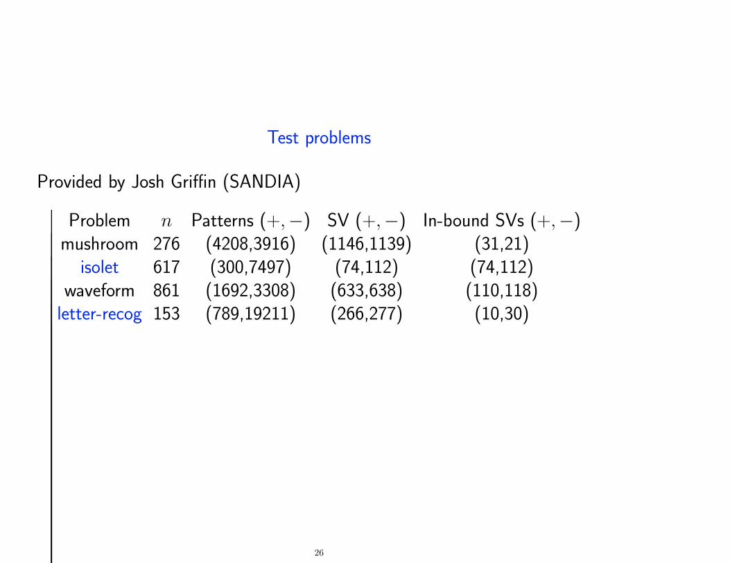
Test problems

Provided by Josh Griffin (SANDIA)

Problem n Patterns (+,−) SV (+,−) In-bound SVs (+,−)mushroom 276 (4208,3916) (1146,1139) (31,21)

isolet 617 (300,7497) (74,112) (74,112)waveform 861 (1692,3308) (633,638) (110,118)

letter-recog 153 (789,19211) (266,277) (10,30)

26

Algorithm variants

We used the reduced predictor-corrector algorithm, with constraints chosenin one of the following ways:

• One-sided distance: Use all points on the wrong side of the boundaryplanes and all points close to the boundary planes.

• Distance: Use all points close to the boundary planes.

• Ω: Use all points with large values of ω−1

i .

We used a balanced selection, choosing approximately equal numbers ofpositive and negative examples.

We compared with no reduction, using all of the terms in forming M.

27

mushroom isolet waveform letter0

5

10

15

20

25

30

35

40Time

Tim

e (s

ec)

Problem

No reductionOne−sided distanceDistance Ωe

28

0.2 0.3 0.4 0.5 0.6 0.7 0.8 0.9 10

5

10

15

20

Tim

e (s

ec)

qU

/m

letter/ distance

0.2 0.3 0.4 0.5 0.6 0.7 0.8 0.9 10

50

100

qU

/m

Itera

tions

letter/ distance

Adaptive balancedAdaptiveNonadaptive balancedNonadaptive

29

0 5 10 15 200

1000

2000

3000

4000

5000

6000

7000

8000

9000

Iterations

# of

pat

tern

s us

ed

mushroom/Adaptive Balanced CR/ distance

qU

= 100%

qU

= 80%

qU

= 60%

qU

= 45%

0 5 10 15 2010

−12

10−10

10−8

10−6

10−4

10−2

100

102

Iterations

µ

mushroom/Adaptive Balanced CR/ distance

No reductionq

U = 100%

qU

= 80%

qU

= 60%

qU

= 45%

30

Comparison with other software

Problem Type LibSVM SVMLight Matlab Oursmushroom Polynomial 5.8 52.2 1280.7mushroom Mapping(Linear) 30.7 60.2 710.1 4.2

isolet Linear 6.5 30.8 323.9 20.1waveform Polynomial 2.9 23.5 8404.1waveform Mapping(Linear) 33.0 85.8 1361.8 16.2

letter Polynomial 2.8 55.8 2831.2letter Mapping(Linear) 11.6 45.9 287.4 13.5

• LibSVM, by Chih-Chung Chang and Chih-Jen Lin, uses a variant ofSMO (by Platt), implemented in C

• SVMLight, by Joachims, implemented in C

• Matlab’s program is a variant of SMO.

• Our program is implemented in Matlab, so a speed-up may bepossible if converted to C.

31

How our algorithm works

To visualize the iteration, we constructed a toy problem with

• n = 2,

• a mapping Φ corresponding to an ellipsoidal separator.

We now show snapshots of the patterns that contribute to M as the IPMiteration proceeds.

32

Iteration: 2, # of obs: 1727

33


34


35


36


37


38


39


40

An extension

Recall that the matrix in the dual problem is H = DAATD, and A ism × n with m >> n.

The elements of K ≡ A A T are

kij = aTi aj,

and our adaptive reduction is efficient because we approximate the termATΩ−1A in the formation of M, which is only n × n.

Often we want a kernel function more general than the inner product, sothat

kij = k(ai, aj).

This would make M m × m.

Efficiency is retained if we can approximate K≈LLT where L has rankmuch less than m. This is often the case, and pivoted Cholesky algorithmshave been used in the literature to compute L.

41

Conclusions

• We have succeeded in significantly improving the training of SVMs thathave large numbers of training points.

• Similar techniques apply to general CQP problems with a large numberof constraints.

• Savings is primarily in later iterations. Future work will focus on usingclustering of patterns (e.g., Boley and Cao (2004)) to reduce work inearly iterations.

42

Documents

SVM May 2007