Survival Analysis Using SPSS

Survival Analysis Using SPSS By Hui Bian

Office for Faculty Excellence

What is survival analysis − Event history analysis − Time series analysis

When use survival analysis − Research interest is about time-to-event and event is discrete

occurrence.

Examples of survival analysis − Duration to the hazard of death − Adoption of an innovation in diffusion research − Marriage duration

Characteristics of survival analysis − At any time point, events may occur − Factors influence events include two types: time-constant and

time-dependent (age).

Survival analysis

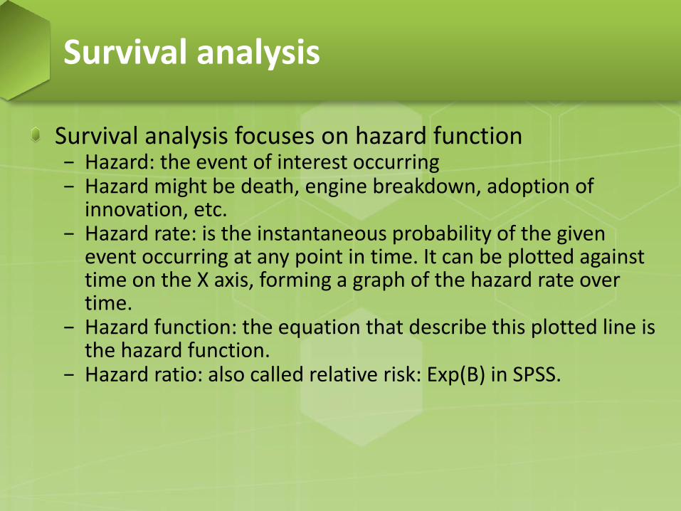
Survival analysis focuses on hazard function − Hazard: the event of interest occurring − Hazard might be death, engine breakdown, adoption of

innovation, etc. − Hazard rate: is the instantaneous probability of the given

event occurring at any point in time. It can be plotted against time on the X axis, forming a graph of the hazard rate over time.

− Hazard function: the equation that describe this plotted line is the hazard function.

− Hazard ratio: also called relative risk: Exp(B) in SPSS.

Survival analysis

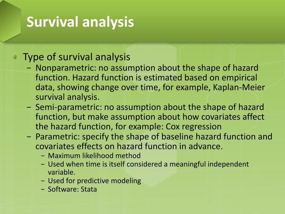
Type of survival analysis − Nonparametric: no assumption about the shape of hazard

function. Hazard function is estimated based on empirical data, showing change over time, for example, Kaplan-Meier survival analysis.

− Semi-parametric: no assumption about the shape of hazard function, but make assumption about how covariates affect the hazard function, for example: Cox regression

− Parametric: specify the shape of baseline hazard function and covariates effects on hazard function in advance.

− Maximum likelihood method − Used when time is itself considered a meaningful independent

variable. − Used for predictive modeling − Software: Stata

Survival analysis

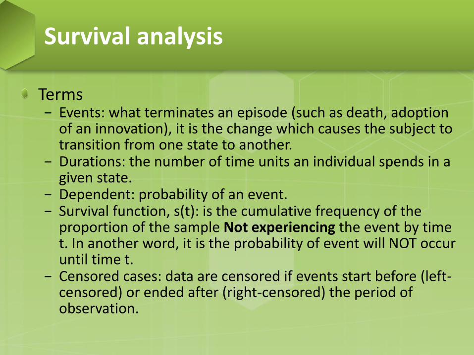
Terms − Events: what terminates an episode (such as death, adoption

of an innovation), it is the change which causes the subject to transition from one state to another.

− Durations: the number of time units an individual spends in a given state.

− Dependent: probability of an event. − Survival function, s(t): is the cumulative frequency of the

proportion of the sample Not experiencing the event by time t. In another word, it is the probability of event will NOT occur until time t.

− Censored cases: data are censored if events start before (left-censored) or ended after (right-censored) the period of observation.

Survival analysis

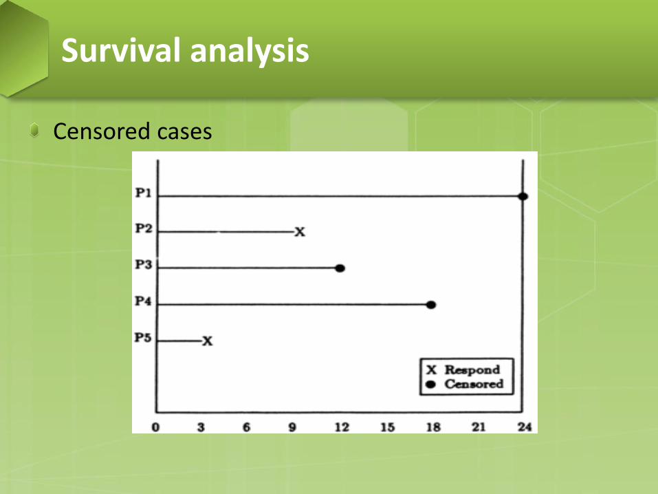
Censored cases

Survival analysis

Censored cases: unique characteristics of survival analysis. − For some cases, the event simply doesn’t occur before the end

of study. − For some cases, they drop out from the study for reasons

unrelated to the study. − For some cases, we lost track of their status sometime before

the end of the study.

Survival analysis

Outline of topics − Life tables − Kaplan-Meier − Cox regression − Cox regression with a time-dependent covariate

Survival analysis

Life Tables is a descriptive procedure for examining the distribution of time-to-event variables. We also can compare the distribution by levels of a factor variable. The basic idea of life tables is to subdivide the period of observation into smaller time intervals. Then the probability from each of the intervals are estimated.

Life tables

Variables − Time variable (duration variable): must be a continuous

variable. − Status variable: binary or categorical variable, represents the

event of interest. − Factor variable: categorical variable.

Assumption − The probability for the event of interest should depend only

on time. Cases that enter the study at different times should behave similarly.

− No systematic differences between censored and uncensored cases

Life tables

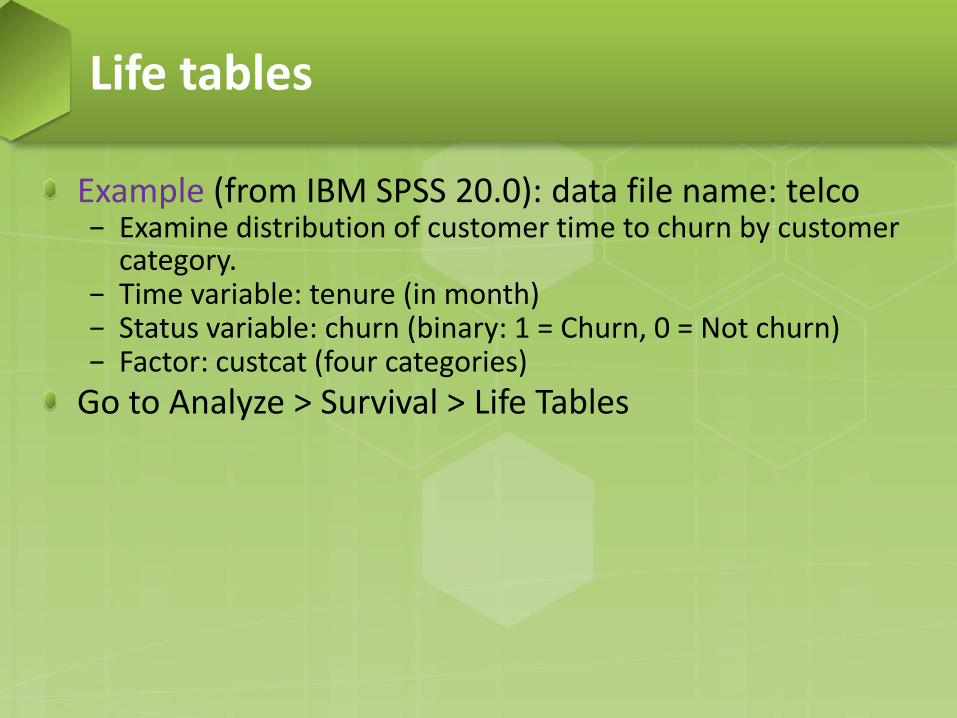
Example (from IBM SPSS 20.0): data file name: telco − Examine distribution of customer time to churn by customer

category. − Time variable: tenure (in month) − Status variable: churn (binary: 1 = Churn, 0 = Not churn) − Factor: custcat (four categories)

Go to Analyze > Survival > Life Tables

Life tables

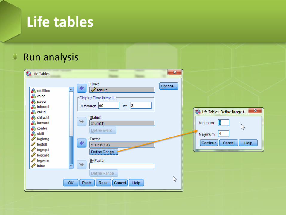
Run analysis

Life tables

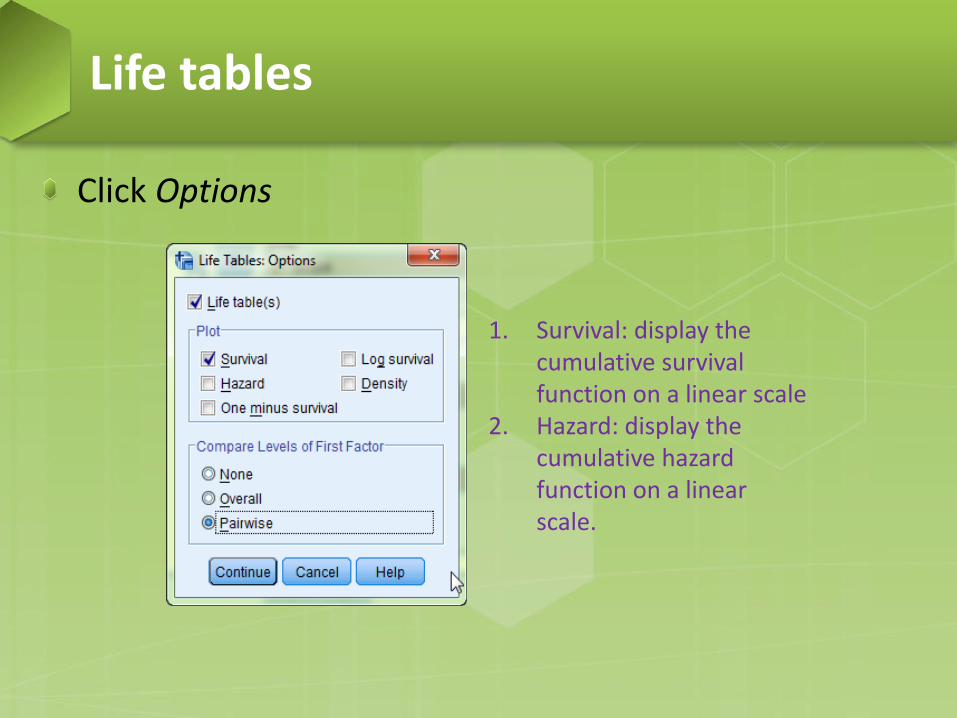
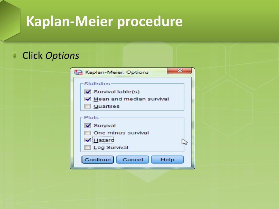
Click Options

Life tables

1. Survival: display the cumulative survival function on a linear scale

2. Hazard: display the cumulative hazard function on a linear scale.

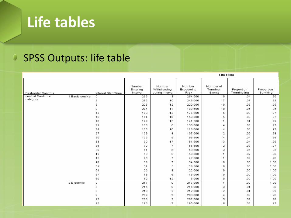
SPSS Outputs: life table

Life tables

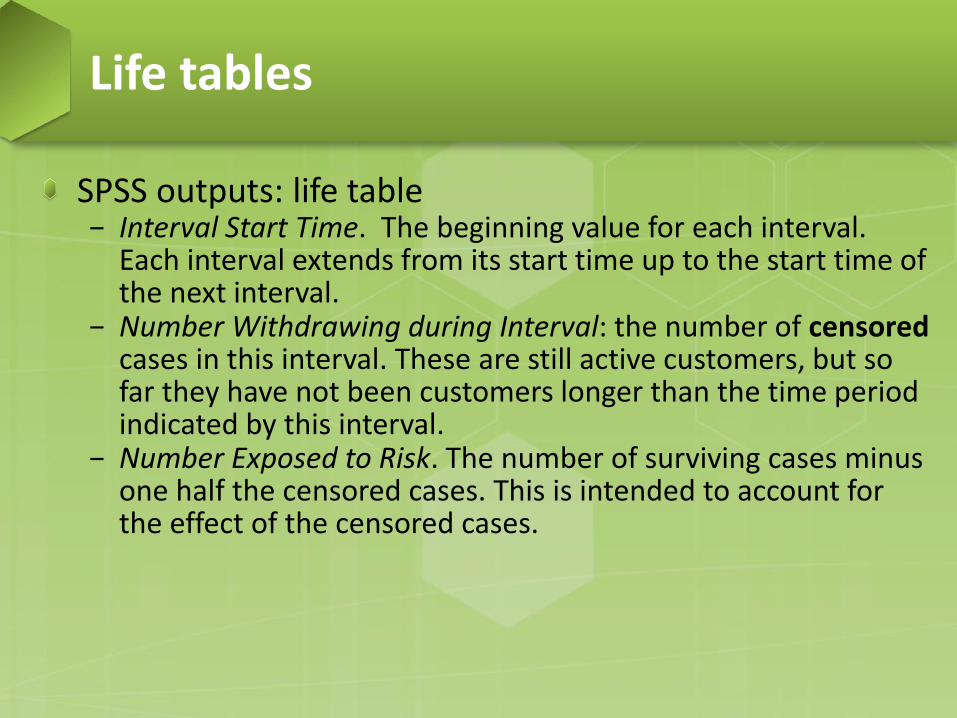
SPSS outputs: life table − Interval Start Time. The beginning value for each interval.

Each interval extends from its start time up to the start time of the next interval.

− Number Withdrawing during Interval: the number of censored cases in this interval. These are still active customers, but so far they have not been customers longer than the time period indicated by this interval.

− Number Exposed to Risk. The number of surviving cases minus one half the censored cases. This is intended to account for the effect of the censored cases.

Life tables

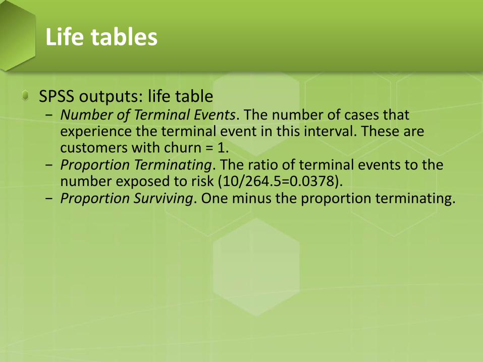
SPSS outputs: life table − Number of Terminal Events. The number of cases that

experience the terminal event in this interval. These are customers with churn = 1.

− Proportion Terminating. The ratio of terminal events to the number exposed to risk (10/264.5=0.0378).

− Proportion Surviving. One minus the proportion terminating.

Life tables

SPSS Outputs: life table

Life tables

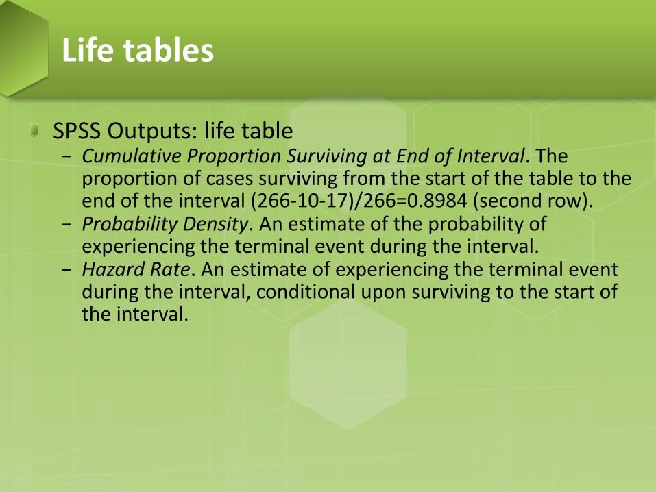
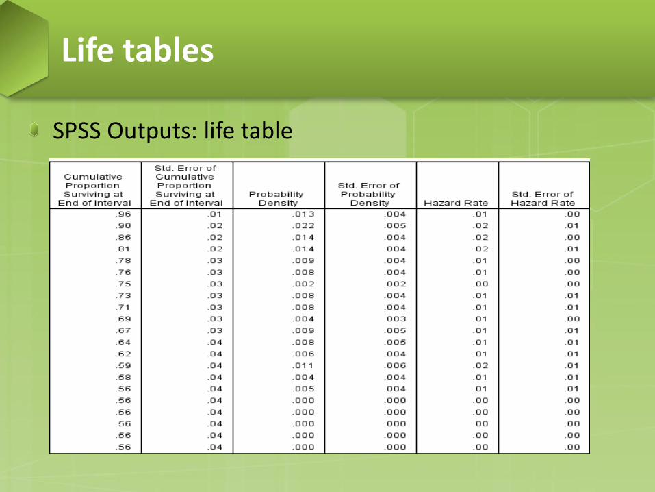
SPSS Outputs: life table − Cumulative Proportion Surviving at End of Interval. The

proportion of cases surviving from the start of the table to the end of the interval (266-10-17)/266=0.8984 (second row).

− Probability Density. An estimate of the probability of experiencing the terminal event during the interval.

− Hazard Rate. An estimate of experiencing the terminal event during the interval, conditional upon surviving to the start of the interval.

Life tables

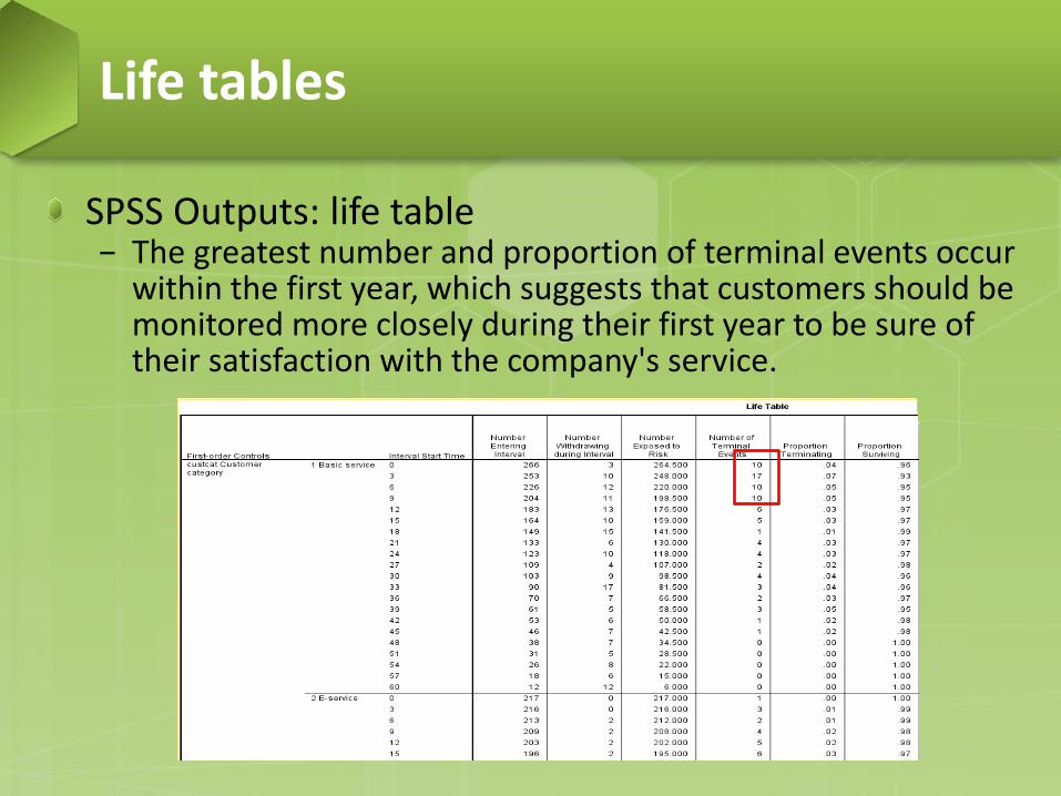
SPSS Outputs: life table − The greatest number and proportion of terminal events occur

within the first year, which suggests that customers should be monitored more closely during their first year to be sure of their satisfaction with the company's service.

Life tables

SPSS Outputs: survival function

Life tables

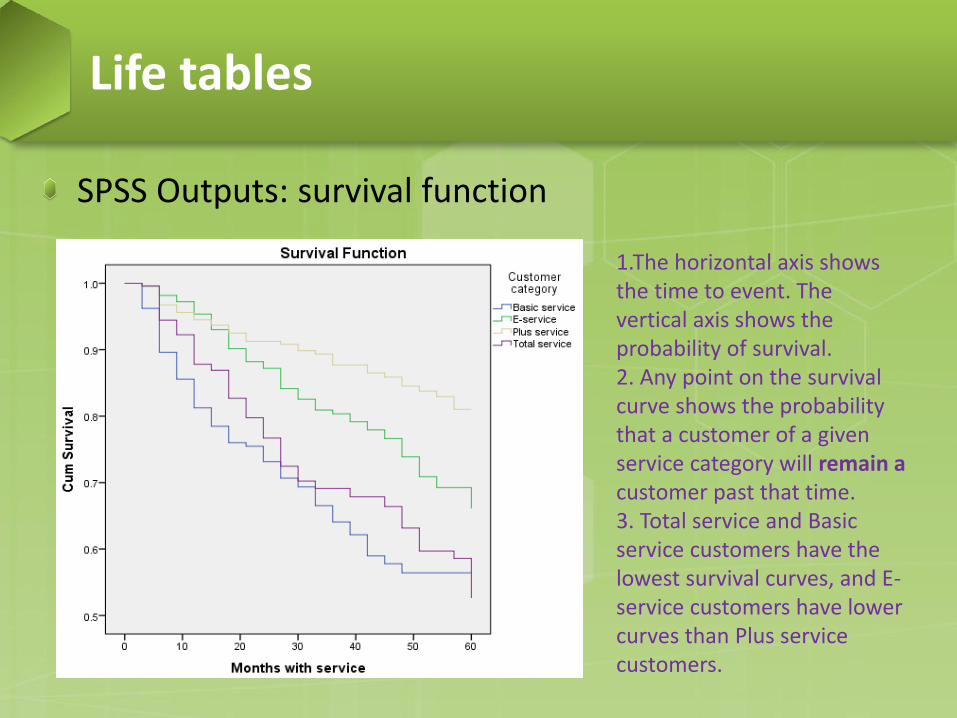
1.The horizontal axis shows the time to event. The vertical axis shows the probability of survival. 2. Any point on the survival curve shows the probability that a customer of a given service category will remain a customer past that time. 3. Total service and Basic service customers have the lowest survival curves, and E-service customers have lower curves than Plus service customers.

SPSS Outputs

Life tables

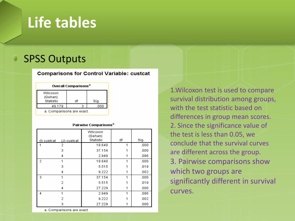
1.Wilcoxon test is used to compare survival distribution among groups, with the test statistic based on differences in group mean scores. 2. Since the significance value of the test is less than 0.05, we conclude that the survival curves are different across the group.

3. Pairwise comparisons show which two groups are significantly different in survival curves.

The Kaplan-Meier procedure is a method of estimating time-to-event models in the presence of censored cases. A descriptive procedure for examining the distribution of time-to-event variables. We also can compare the distribution by levels of a factor variable or produce separate analyses by levels of a stratification variable. Censored cases (right-censored cases) are those for which the event of interest has not yet happened.

Kaplan-Meier procedure

Assumptions − Probabilities for the event of interest should depend only on

time after the initial event without covariates effects. − Cases that enter the study at different times (for example,

patients who begin treatment at different times) should behave similarly.

− Censored and uncensored cases behave the same. If, for example, many of the censored cases are patients with more serious conditions, your results may be biased.


Example (from IBM SPSS 20.0) : data file: pain_medication − A pharmaceutical company is developing an anti-inflammatory

medication for treating chronic arthritic pain. The research interest is the time it takes for the drug to take effect and how it compares to an existing drug. Shorter times to effect are considered better.

Event: drug takes effect


Variables − Time variable (duration variable): must be a continuous

variable − Status variable: categorical or continuous variable, represents

the event of interest (drug has effect or not). − Factor variable: categorical variable, represents a causal effect

(type of treatment for example). − Stratification variable: categorical variable.


We have Factor variable: Treatment (0 = New drug, 1 = old drug), Status variable: status ( 0 = censored, 1 = take effect), Time variable: time We want to compare the effect of two different drugs. Null hypothesis: whether survival function is the same between different levels of the factor variable (between old and new drug) .


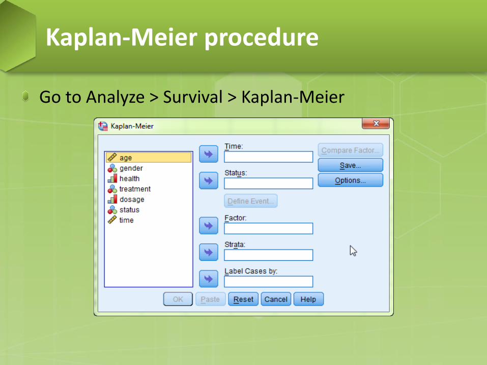
Go to Analyze > Survival > Kaplan-Meier


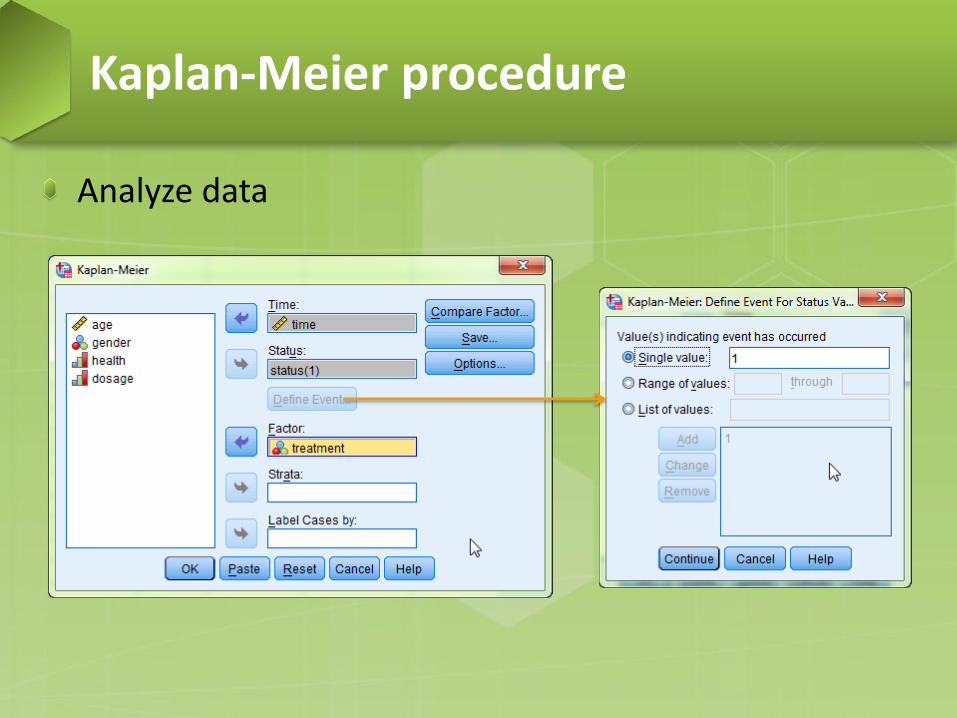
Analyze data


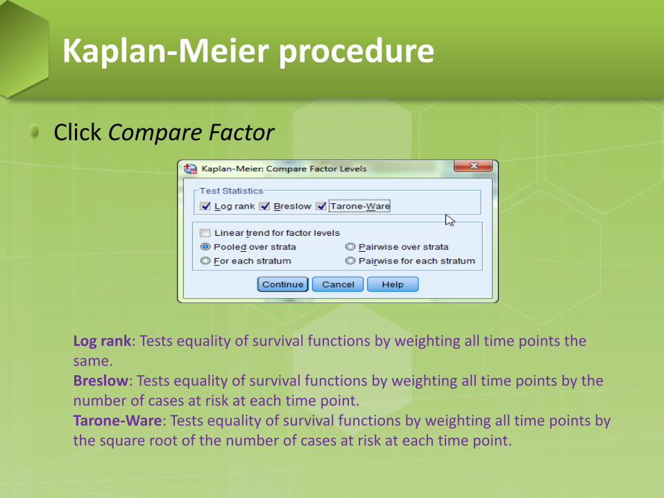
Click Compare Factor


Log rank: Tests equality of survival functions by weighting all time points the same. Breslow: Tests equality of survival functions by weighting all time points by the number of cases at risk at each time point. Tarone-Ware: Tests equality of survival functions by weighting all time points by the square root of the number of cases at risk at each time point.

Compare factor


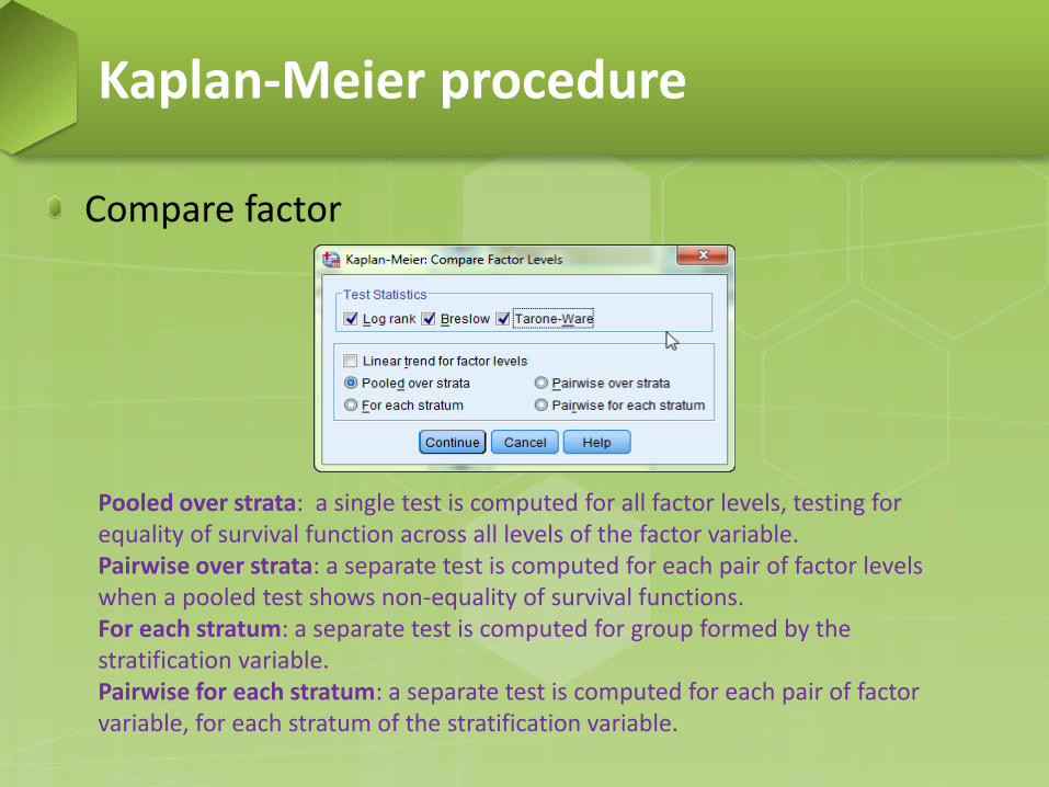
Pooled over strata: a single test is computed for all factor levels, testing for equality of survival function across all levels of the factor variable. Pairwise over strata: a separate test is computed for each pair of factor levels when a pooled test shows non-equality of survival functions. For each stratum: a separate test is computed for group formed by the stratification variable. Pairwise for each stratum: a separate test is computed for each pair of factor variable, for each stratum of the stratification variable.

Click Options


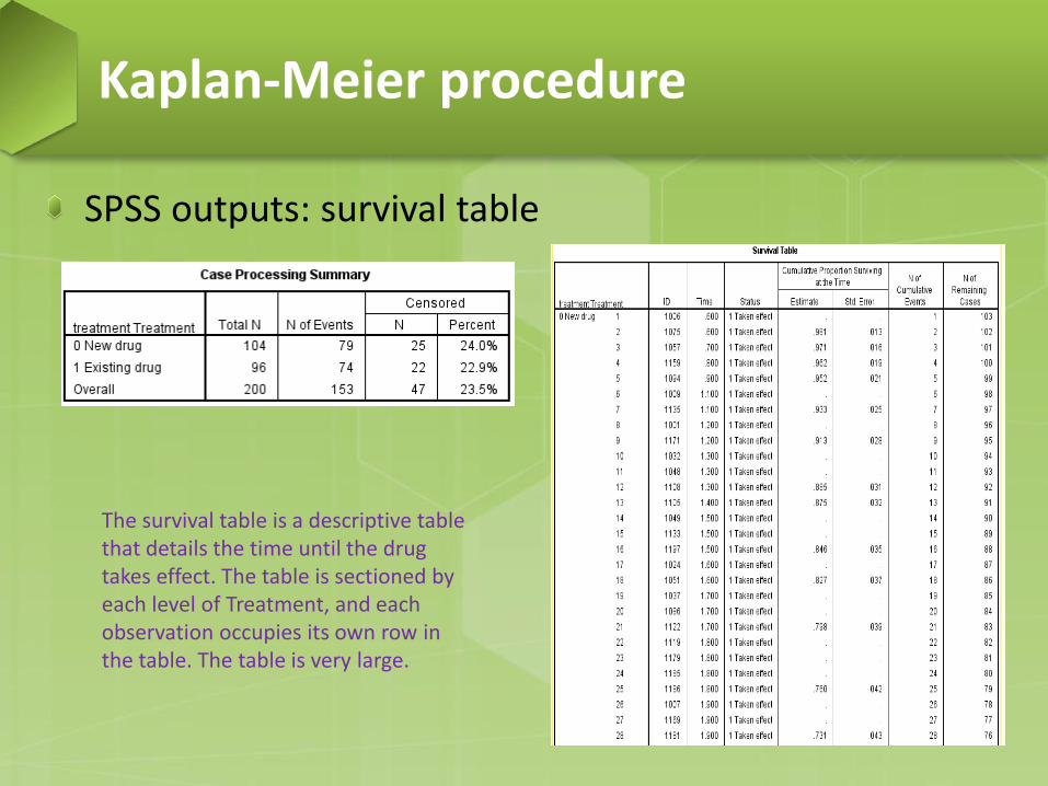
SPSS outputs: survival table


The survival table is a descriptive table that details the time until the drug takes effect. The table is sectioned by each level of Treatment, and each observation occupies its own row in the table. The table is very large.

Survival table − Time. The time at which the event or censoring occurred. − Status. Indicates whether the case experienced the terminal

event or was censored. − Cumulative Proportion Surviving at the Time. The proportion

of cases surviving from the start of the table until this time. When multiple cases experience the terminal event at the same time, these estimates are printed once for that time period and apply to all the cases whose drug took effect at that time.


Survival table − N of Cumulative Events. The number of cases that have

experienced the terminal event from the start of the table until this time.

− N of Remaining Cases. The number of cases that, at this time, haven’t yet to experience the terminal event or be censored.


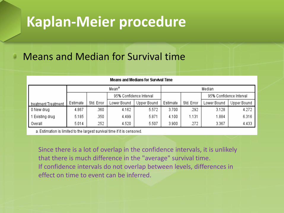
Means and Median for Survival time


Since there is a lot of overlap in the confidence intervals, it is unlikely that there is much difference in the "average" survival time. If confidence intervals do not overlap between levels, differences in effect on time to event can be inferred.

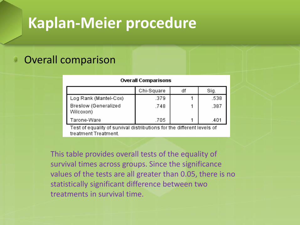
Overall comparison


This table provides overall tests of the equality of survival times across groups. Since the significance values of the tests are all greater than 0.05, there is no statistically significant difference between two treatments in survival time.

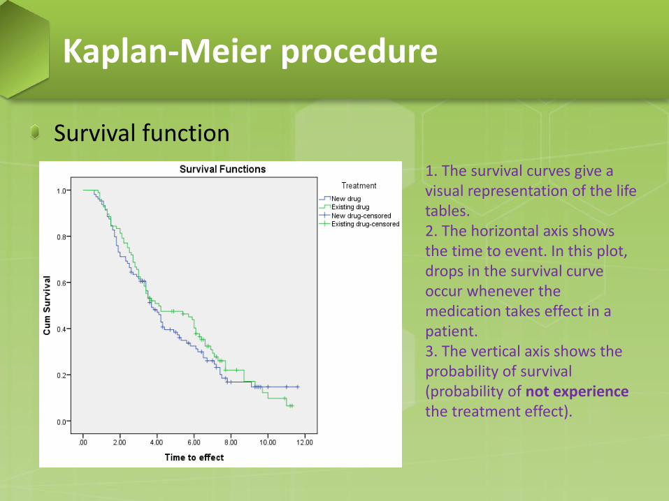
Survival function


1. The survival curves give a visual representation of the life tables. 2. The horizontal axis shows the time to event. In this plot, drops in the survival curve occur whenever the medication takes effect in a patient. 3. The vertical axis shows the probability of survival (probability of not experience the treatment effect).

The Cox Regression procedure is useful for modeling the time to a specified event, based upon the values of given covariates. One or more covariates are used to predict a status (event). The central statistical output is the hazard ratio. Data contain censored and uncensored cases. Similar to logistic regression, but Cox regression assesses relationship between survival time and covariates .

Cox regression

Terms − Status variable: the dependent in Cox regression, should be

binary variable. − Time variable: measures duration to the event defined by the

status variable (continuous or discrete). − Covariates: independent/predictor variables. They can be

categorical or continuous. They also can be time-fixed or time-dependent.

− Interaction terms − Categorical covariates: SPSS automatically convert them into a set of

dummy variables, omitting one category.

Cox regression

Example (from SPSS): data file: telco − Use Cox Regression to determine which attributes are

associated with shorter "time to churn“. − Time variable: tenure (month with services) − Status variable: churn (0 = No, 1 = Yes). − Covariates: age, marital, address, employ, retire, gender,

reside, and custcat

Go to Analyze > Survival > Cox Regression

Cox regression

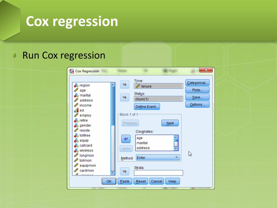
Run Cox regression

Cox regression

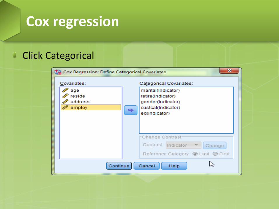
Click Categorical

Cox regression

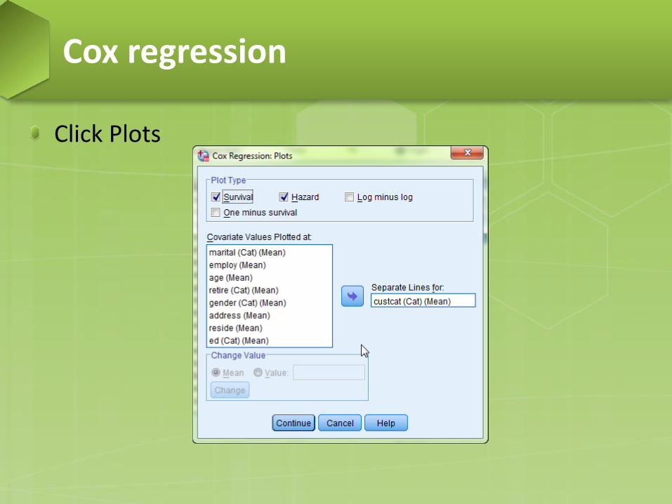
Click Plots

Cox regression

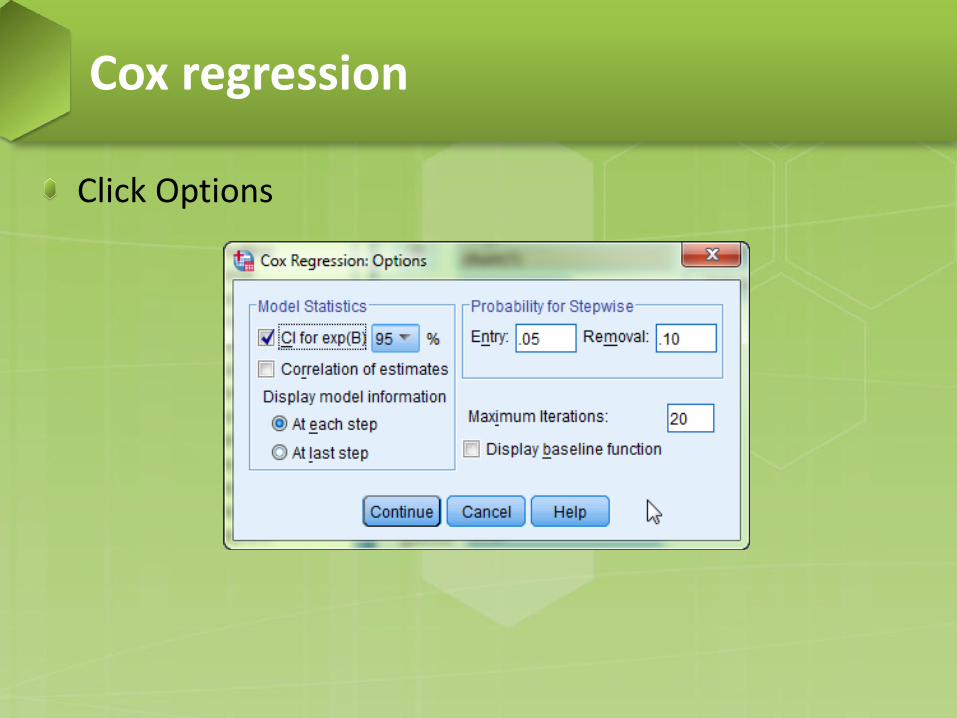
Click Options

Cox regression

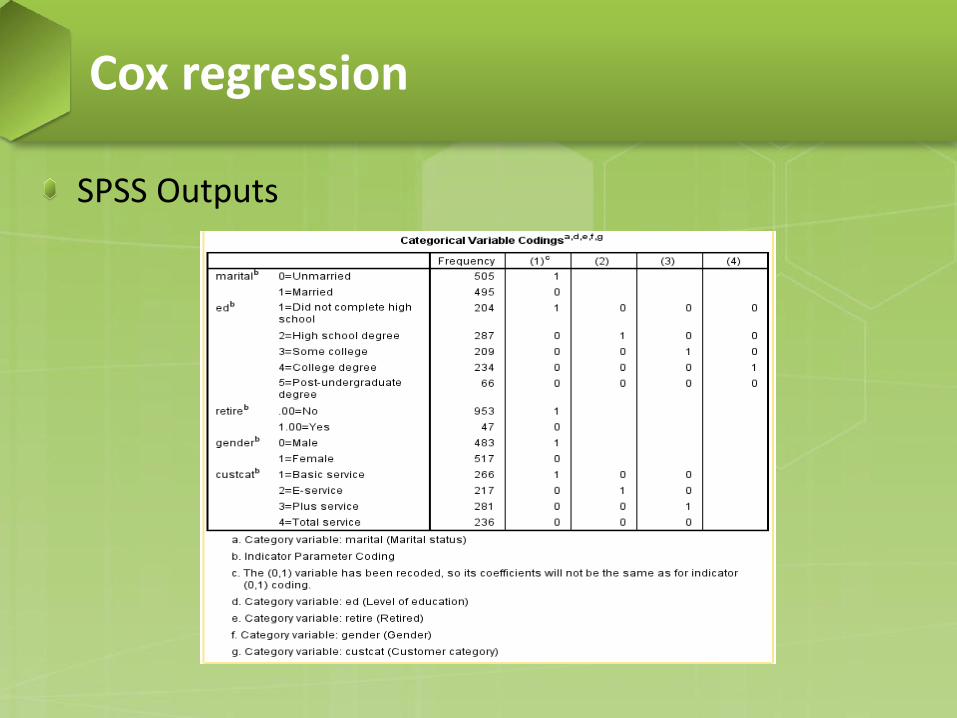
SPSS Outputs

Cox regression

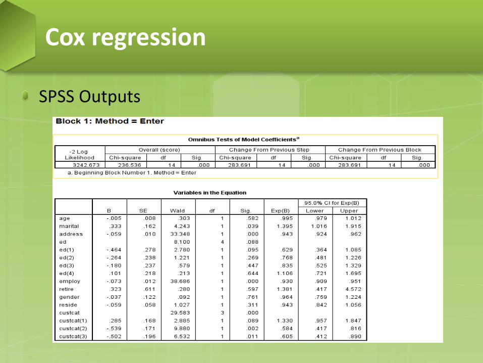
SPSS Outputs

Cox regression

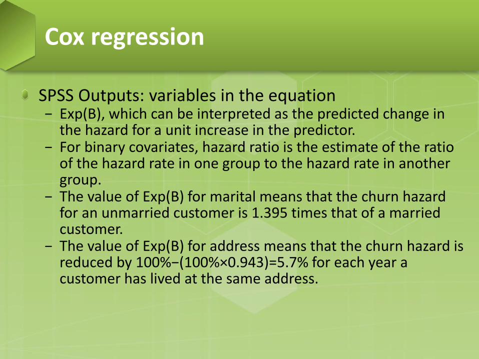
SPSS Outputs: variables in the equation − Exp(B), which can be interpreted as the predicted change in

the hazard for a unit increase in the predictor. − For binary covariates, hazard ratio is the estimate of the ratio

of the hazard rate in one group to the hazard rate in another group.

− The value of Exp(B) for marital means that the churn hazard for an unmarried customer is 1.395 times that of a married customer.

− The value of Exp(B) for address means that the churn hazard is reduced by 100%−(100%×0.943)=5.7% for each year a customer has lived at the same address.

Cox regression

SPSS Outputs

Cox regression

This table displays the average value of each predictor variable, plus a pattern for each level of custcat. The four patterns correspond to each of the customer types, each with otherwise "average" predictor values.

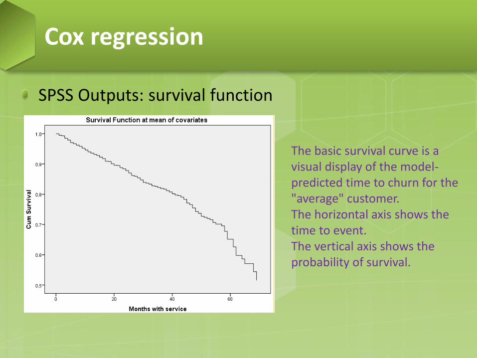
SPSS Outputs: survival function

Cox regression

The basic survival curve is a visual display of the model-predicted time to churn for the "average" customer. The horizontal axis shows the time to event. The vertical axis shows the probability of survival.

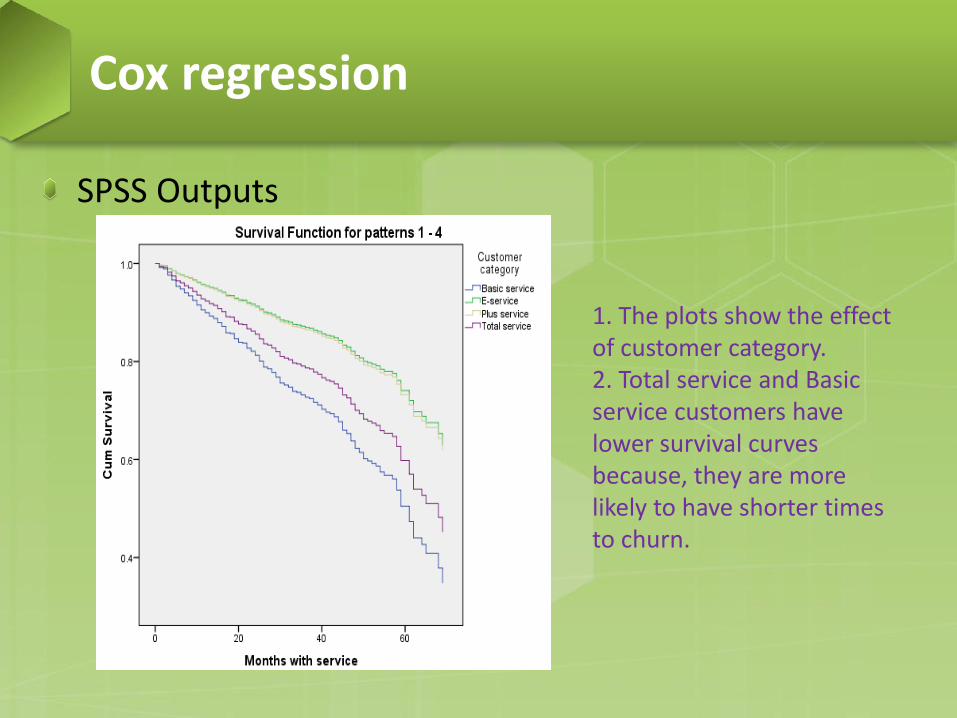
SPSS Outputs

Cox regression

1. The plots show the effect of customer category. 2. Total service and Basic service customers have lower survival curves because, they are more likely to have shorter times to churn.

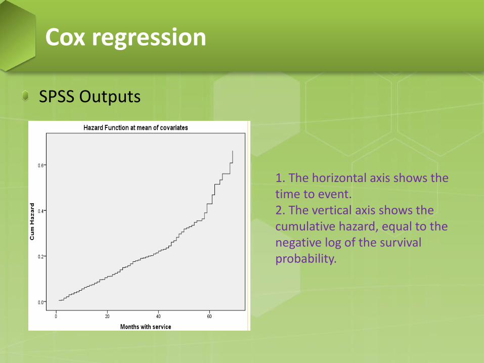
SPSS Outputs

Cox regression

1. The horizontal axis shows the time to event. 2. The vertical axis shows the cumulative hazard, equal to the negative log of the survival probability.

Time-dependent covariates − Simple product of the time variable and the covariate. − Some variables may have different values at different time

periods but aren't systematically related to time. In such cases, you need to define a segmented time-dependent covariate, which can be done using logical expressions.

Cox regression with a time-dependent covariate

Example (from IBM SPSS 20.0): data file: recidivism − A government law enforcement agency is concerned about

recidivism rates in their area of jurisdiction. One of the measures of recidivism is the time until second arrest for offenders. The agency would like to model time to rearrest using Cox Regression, but are worried the proportional hazards assumption is invalid across age categories.

Go to Analyze > Survival > Cox with time-dependent covariate

Cox regression with a time-dependent covariates

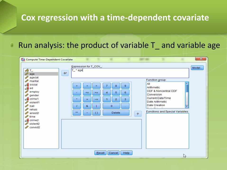
Run analysis: the product of variable T_ and variable age


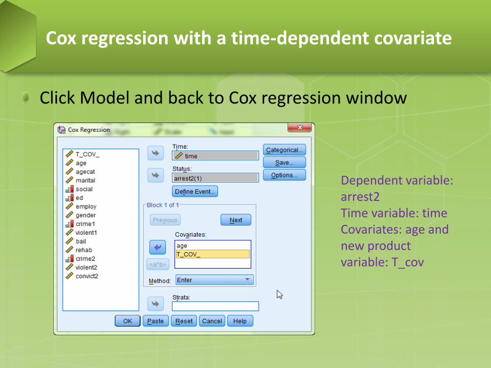
Click Model and back to Cox regression window


Dependent variable: arrest2 Time variable: time Covariates: age and new product variable: T_cov

SPSS outputs


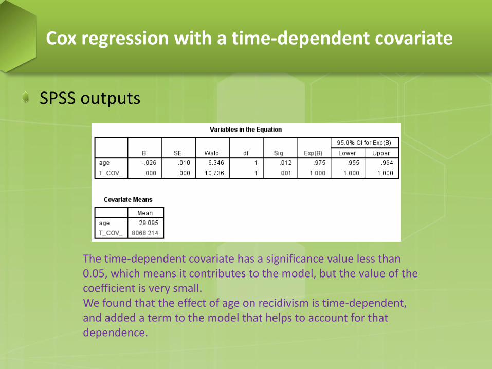
The time-dependent covariate has a significance value less than 0.05, which means it contributes to the model, but the value of the coefficient is very small. We found that the effect of age on recidivism is time-dependent, and added a term to the model that helps to account for that dependence.

Documents

Survival Analysis Using SPSS