Embed Size (px)
Citation preview

Repeated measures ANOVA in SPSSCross tabulationsSurvival analysis

Repeated measures ANOVA in SPSS
2

The data from Chen 2004
• The number of errors are recorded for the same test repeated 4 times
• The degree of anxiety was different between the subjects.
• Stuff we would like to know:• Is there a difference in the
performance between the anxiety groups?
• Is there a reduction in errors over time – a learning effect?
• Does one of the groups learn faster than the other?
3
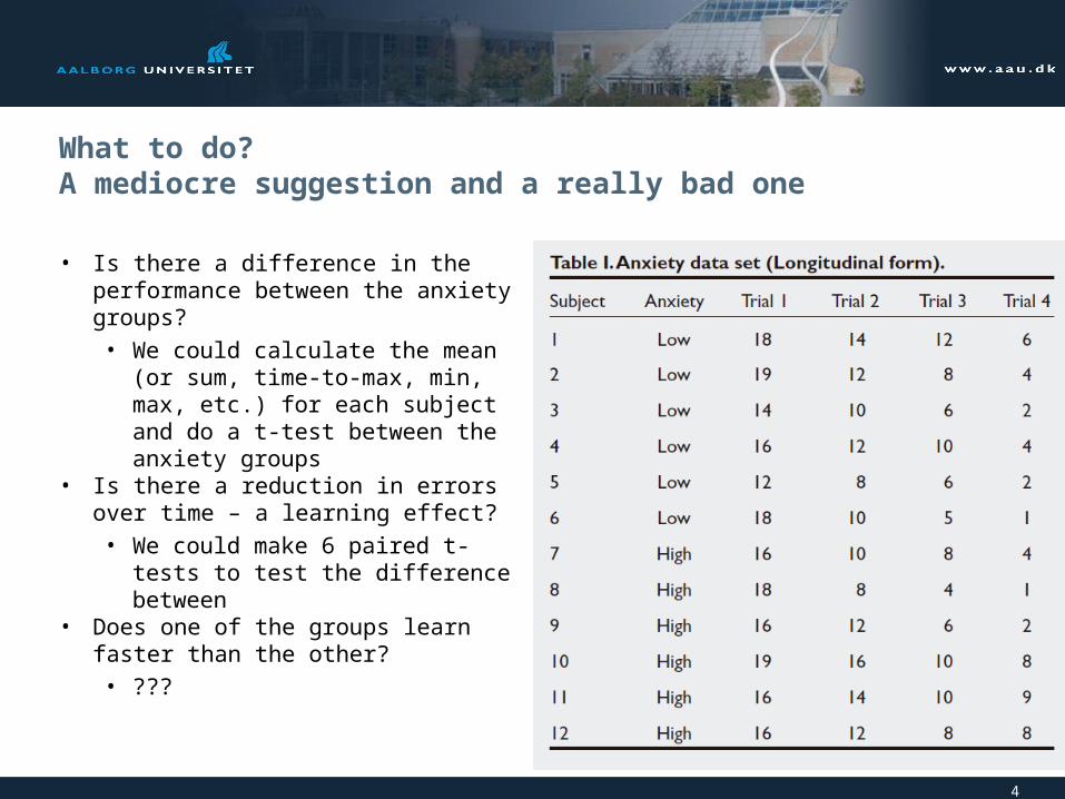
What to do? A mediocre suggestion and a really bad one
• Is there a difference in the performance between the anxiety groups?• We could calculate the mean
(or sum, time-to-max, min, max, etc.) for each subject and do a t-test between the anxiety groups
• Is there a reduction in errors over time – a learning effect?• We could make 6 paired t-tests
to test the difference between • Does one of the groups learn
faster than the other?• ???
4
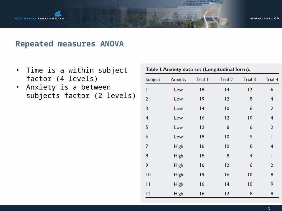
Repeated measures ANOVA
• Time is a within subject factor (4 levels)
• Anxiety is a between subjects factor (2 levels)
5

Repeated measures ANOVA
• Plotting the data
6
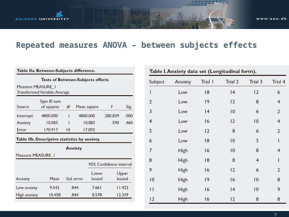
Repeated measures ANOVA – between subjects effects
7
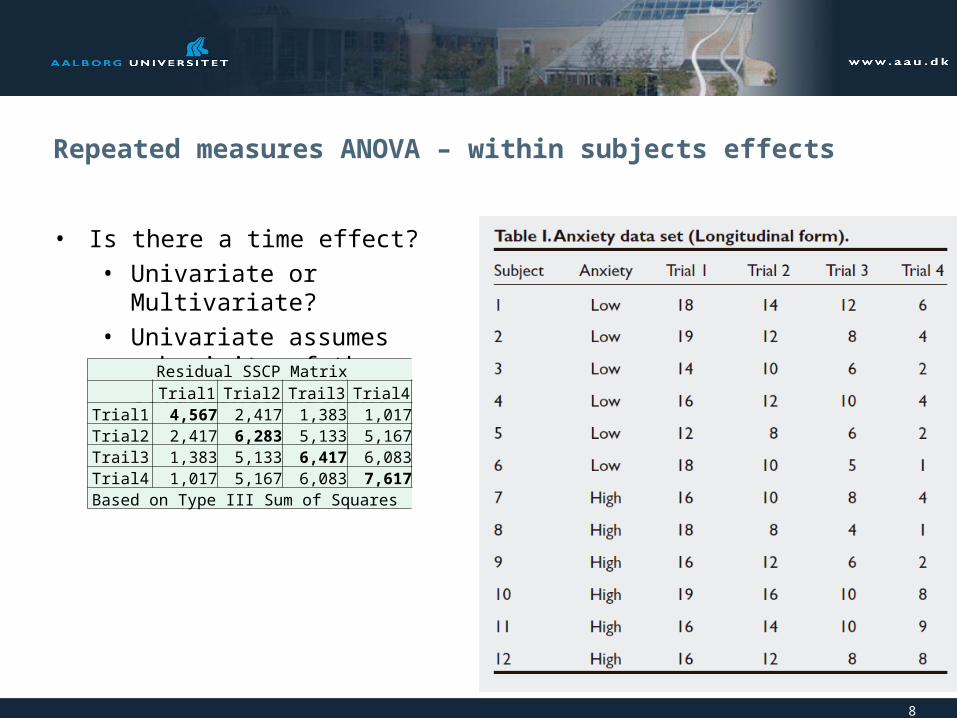
Repeated measures ANOVA – within subjects effects
• Is there a time effect?• Univariate or Multivariate?• Univariate assumes
sphericity of the covariance matrix:
8
Residual SSCP Matrix Trial1 Trial2 Trail3 Trial4
Trial1 4,567 2,417 1,383 1,017Trial2 2,417 6,283 5,133 5,167Trail3 1,383 5,133 6,417 6,083Trial4 1,017 5,167 6,083 7,617Based on Type III Sum of Squares

Repeated measures ANOVA – within subjects effectsUnivariate
Mauchly's Test of Sphericityb
Measure:MEASURE_1Within Subjects Effect Mauchly'
s W
Approx. Chi-
Square df Sig.dimensio
n1time ,337 9,496 5 ,093
Tests the null hypothesis that the error covariance matrix of the orthonormalized transformed dependent variables is proportional to an identity matrix. b. Design: Intercept + Anxiety Within Subjects Design: time 9
Residual SSCP Matrix Trial1 Trial2 Trail3 Trial4
Trial1 4,567 2,417 1,383 1,017Trial2 2,417 6,283 5,133 5,167Trail3 1,383 5,133 6,417 6,083Trial4 1,017 5,167 6,083 7,617Based on Type III Sum of Squares

Repeated measures ANOVA – within subjects effectsUnivariate
10
• Greenhouse-Geisser is newer than Huynh-Feldt methods• Lower-bound is the most konservative• Alternatively use Multible ANOVA

Repeated measures ANOVA – within subjects effectsMultivariate
11
• The covariance matrices must be equal for all levels of the between groups
• Tested by Box’s test
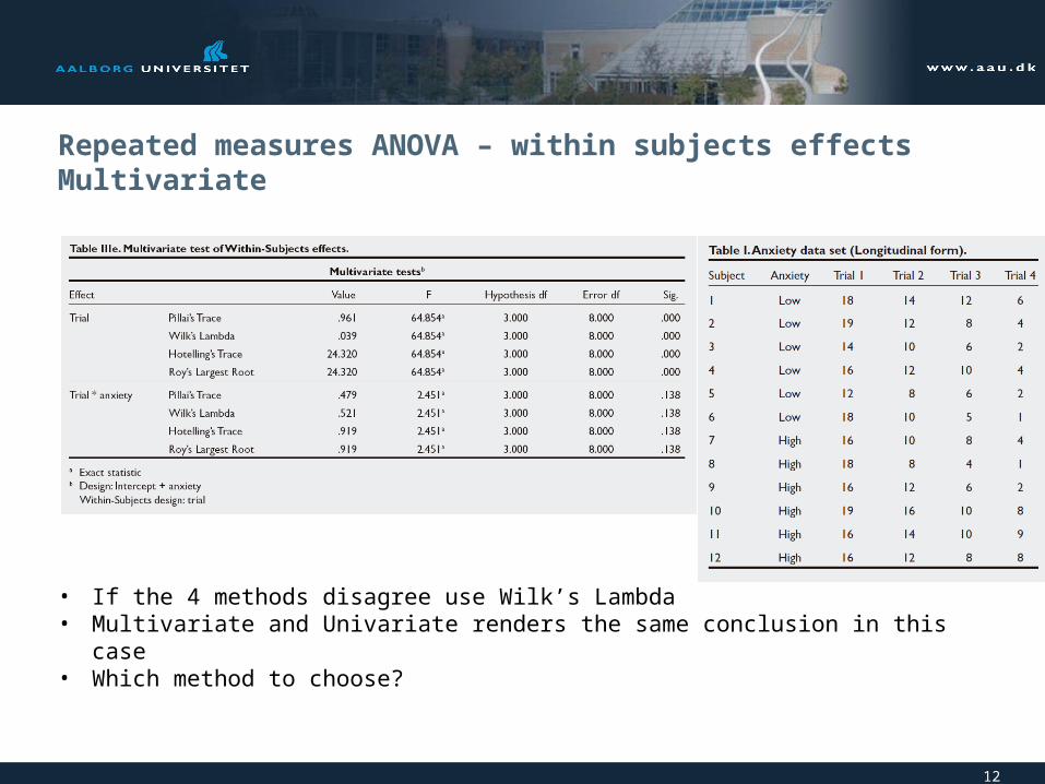
Repeated measures ANOVA – within subjects effectsMultivariate
12
• If the 4 methods disagree use Wilk’s Lambda• Multivariate and Univariate renders the same conclusion in this case• Which method to choose?
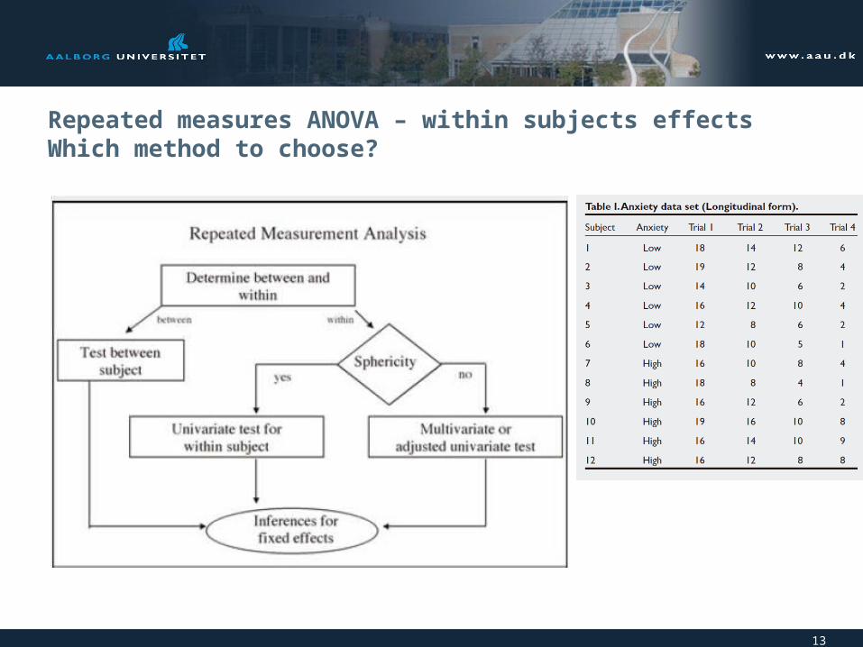
Repeated measures ANOVA – within subjects effectsWhich method to choose?
13

Repeated measures ANOVA – within subjects effectsPairwise comparisons
14
• Does all these comparisons make sense?

Repeated measures ANOVA – within subjects effectsContrasts?
15

Cross tabulations
16
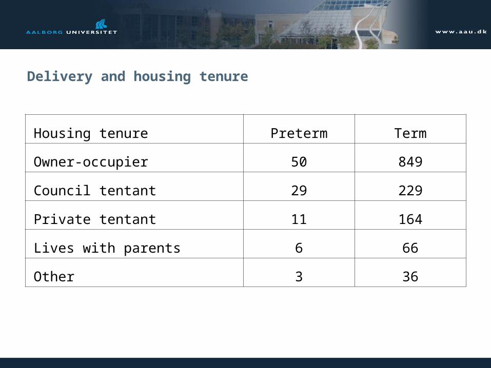
Delivery and housing tenure
Housing tenure Preterm Term
Owner-occupier 50 849
Council tentant 29 229
Private tentant 11 164
Lives with parents 6 66
Other 3 36

Cross-tabulations
Tables of countable entities or frequencies Made to analyze the association, relationship, or connection between
two variables This association is difficult to describe statistically Null- Hypothesis: “There is no association between the two variables”
can be tested Analysis of cross-tabulations with larges samples

Delivery and housing tenure
Housing tenure Preterm Term Total
Owner-occupier 50 849 899
Council tentant 29 229 258
Private tentant 11 164 175
Lives with parents 6 66 72
Other 3 36 39
Total 99 1344 1443
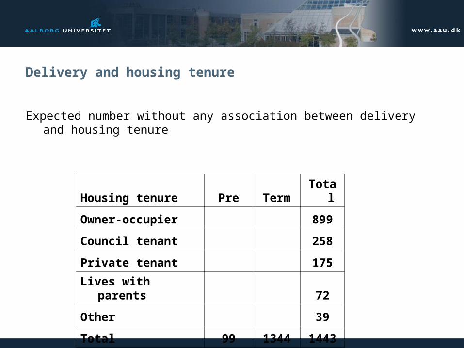
Delivery and housing tenure
Expected number without any association between delivery and housing tenure
Housing tenure Pre Term Total
Owner-occupier 899
Council tenant 258
Private tenant 175
Lives with parents 72
Other 39
Total 99 1344 1443

Delivery and housing tenureIf the null-hypothesis is true
899/1443 = 62.3% are house owners.62.3% of the Pre-terms should be house owners: 99*899/1443 = 61.7
Housing tenure Pre Term Total
Owner-occupier 899
Council tenant 258
Private tenant 175
Lives with parents 72
Other 39
Total 99 1344 1443

Delivery and housing tenureIf the null-hypothesis is true
899/1443 = 62.3% are house owners.62.3% of the ‘Term’s should be house owners: 1344*899/1443 =
837.3
Housing tenure Pre Term Total
Owner-occupier 61.7 899
Council tenant 258
Private tenant 175
Lives with parents 72
Other 39
Total 99 1344 1443

Delivery and housing tenureIf the null-hypothesis is true
258/1443 = 17.9% are council tenant.17.9% of the ‘preterm’s should be council tenant: 99*258/1443 =
17.7
Housing tenure Pre Term Total
Owner-occupier 61.7 837.3 899
Council tenant 258
Private tenant 175
Lives with parents 72
Other 39
Total 99 1344 1443
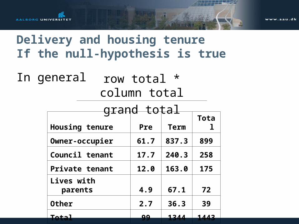
Delivery and housing tenureIf the null-hypothesis is true
In general
Housing tenure Pre Term Total
Owner-occupier 61.7 837.3 899
Council tenant 17.7 240.3 258
Private tenant 12.0 163.0 175
Lives with parents 4.9 67.1 72
Other 2.7 36.3 39
Total 99 1344 1443
row total * column total
grand total

Delivery and housing tenureIf the null-hypothesis is true
Housing tenure Pre Term Total
Owner-occupier 50(61.7) 849(837.3) 899
Council tenant 29(17.7) 229(240.3) 258
Private tenant 11(12.0) 164(163.0) 175
Lives with parents 6(4.9) 66(67.1) 72
Other 3(2.7) 36(36.3) 39
Total 99 1344 1443
2
all_cells
10.5O E
E

Delivery and housing tenuretest for association
If the numbers are large this will be chi-square distributed.The degree of freedom is (r-1)(c-1) = 4From Table 13.3 there is a 1 - 5% probability that delivery and
housing tenure is not associated
2
all_cells
10.5O E
E

Chi Squared Table

Delivery and housing tenureIf the null-hypothesis is true
It is difficult to say anything about the nature of the association.
Housing tenure Pre Term Total
Owner-occupier 50(61.7) 849(837.3) 899
Council tenant 29(17.7) 229(240.3) 258
Private tenant 11(12.0) 164(163.0) 175
Lives with parents 6(4.9) 66(67.1) 72
Other 3(2.7) 36(36.3) 39
Total 99 1344 1443

Chi-squared test for small samples
Expected valued• > 80% >5• All >1
Streptomycin Control Total
Improvement 13 (8.4) 5 (9.6) 18
Deterioration 2 (4.2) 7 (4.8) 9
Death 0 (2.3) 5 (2.7) 5
Total 15 17 32
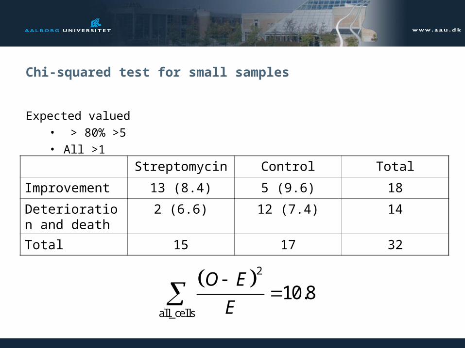
Chi-squared test for small samples
Expected valued• > 80% >5• All >1
Streptomycin Control Total
Improvement 13 (8.4) 5 (9.6) 18
Deterioration and death
2 (6.6) 12 (7.4) 14
Total 15 17 32
2
all_cells
10.8O E
E
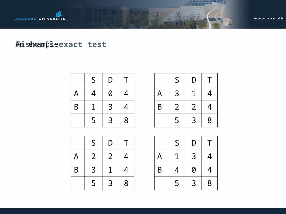
Fisher’s exact testAn example
S D T
A 3 1 4
B 2 2 4
5 3 8
S D T
A 4 0 4
B 1 3 4
5 3 8
S D T
A 1 3 4
B 4 0 4
5 3 8
S D T
A 2 2 4
B 3 1 4
5 3 8
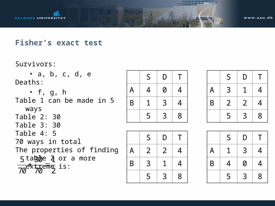
Fisher’s exact test
Survivors: • a, b, c, d, e
Deaths: • f, g, h
Table 1 can be made in 5 waysTable 2: 30Table 3: 30Table 4: 570 ways in totalThe properties of finding table 2
or a more extreme is:
S D T
A 3 1 4
B 2 2 4
5 3 8
S D T
A 4 0 4
B 1 3 4
5 3 8
S D T
A 1 3 4
B 4 0 4
5 3 8
S D T
A 2 2 4
B 3 1 4
5 3 8
5 30 1
70 70 2
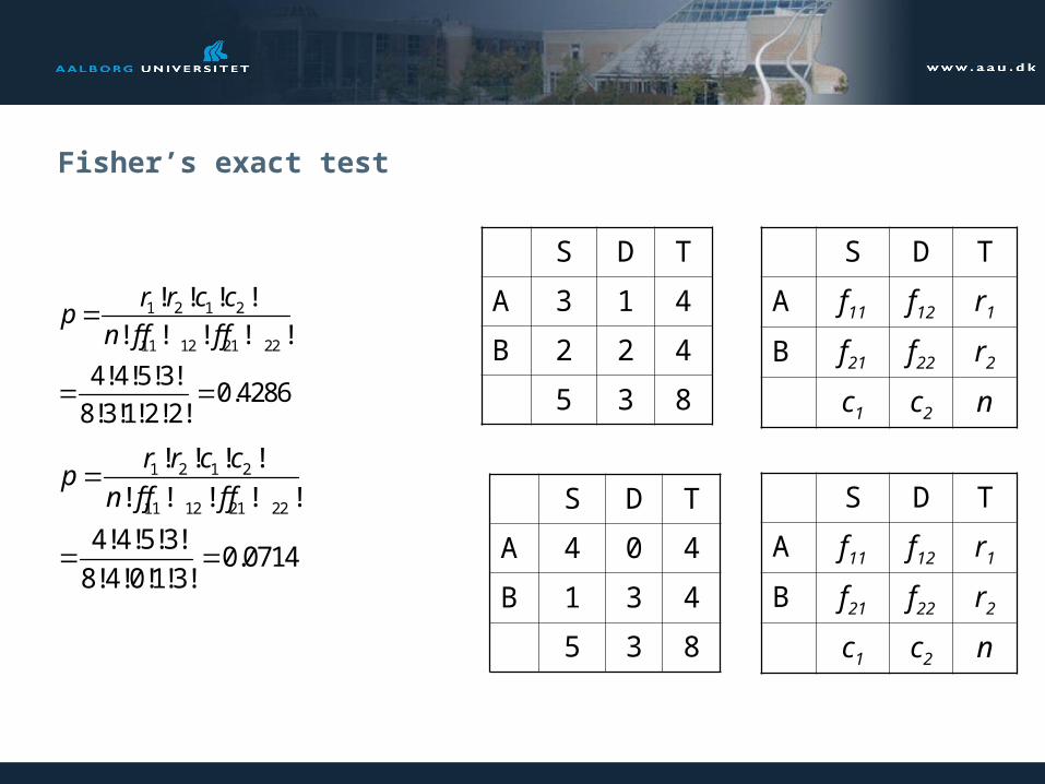
Fisher’s exact test
S D T
A f11 f12 r1
B f21 f22 r2
c1 c2 n
S D T
A 3 1 4
B 2 2 4
5 3 8
1 2 1 2
11 12 21 22
! ! ! !
! ! ! ! !
4!4!5!3!0.4286
8!3!1!2!2!
r r c cp
n f f f f
S D T
A f11 f12 r1
B f21 f22 r2
c1 c2 n
S D T
A 4 0 4
B 1 3 4
5 3 8
1 2 1 2
11 12 21 22
! ! ! !
! ! ! ! !
4!4!5!3!0.0714
8!4!0!1!3!
r r c cp
n f f f f
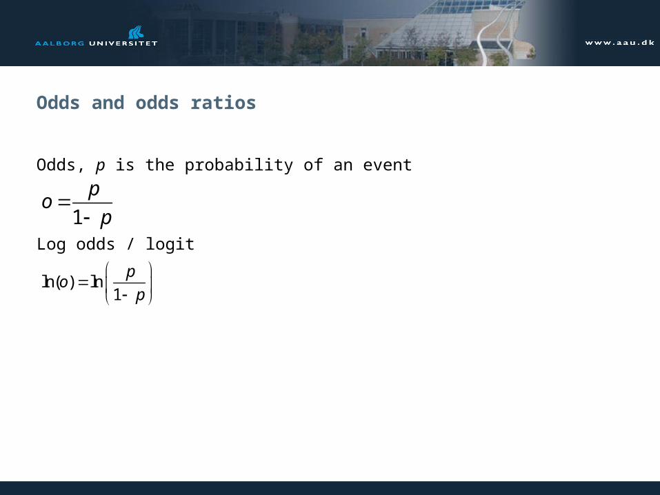
Odds and odds ratios
Odds, p is the probability of an event
Log odds / logit
1
po
p
ln( ) ln1
po
p

Odds
The probability of coughs in kids with history of bronchitis.p = 26/273 = 0.095o = 26/247 = 0.105
The probability of coughs in kids with history without bronchitis.
p = 44/1046 = 0.042o = 44/1002 = 0.044
Bronchitis No bronchitis Total
Cough 26 (a) 44 (b) 70
No Cough 247 (c) 1002 (d) 1249
Total 273 1046 1319
1
po
p

Odds ratio
The odds ratio; the ratio of odds for experiencing coughs in kids with and kids without a history of bronchitis.
Bronchitis No bronchitis Total
Cough 26; 0.105 (a) 44; 0.0439 (b) 70
No Cough 247; 9.50 (c) 1002; 22.8 (d) 1249
Total 273 1046 1319
ac
bd
ador
bc
ab
cd
ador
bc
26247
441002
26*10022.40
247*44or
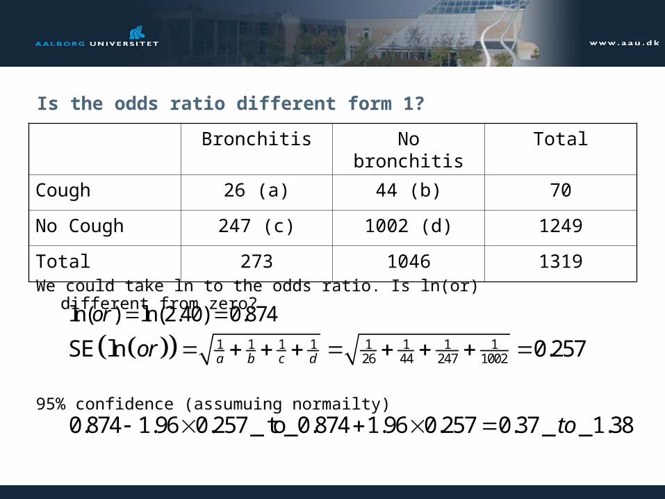
Is the odds ratio different form 1?
Bronchitis No bronchitis Total
Cough 26 (a) 44 (b) 70
No Cough 247 (c) 1002 (d) 1249
Total 273 1046 1319
1 1 1 1 1 1 1 126 44 247 1002SE ln 0.257a b c dor
0.874 1.96 0.257 _ to_0.874 1.96 0.257 0.37 _ _1.38to
ln( ) ln(2.40) 0.874or We could take ln to the odds ratio. Is ln(or) different from
zero?
95% confidence (assumuing normailty)

Confidence interval of the Odds ratio
ln (or) ± 1.96*SE(ln(or)) = 0.37 to 1.38Returning to the odds ratio itself:e0.370 to e1.379 = 1.45 to 3.97The interval does not contain 1, indicating a statistically significant
difference
Bronchitis No bronchitis Total
Cough 26 (a) 44 (b) 70
No Cough 247 (c) 1002 (d) 1249
Total 273 1046 1319
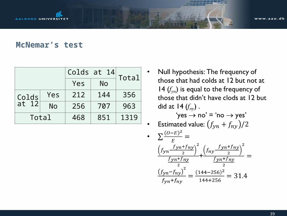
McNemar’s test
Colds at 14
TotalYes No
Colds at 12
Yes 212 144 356
No 256 707 963
Total 468 851 1319
39

Survival analysis
40
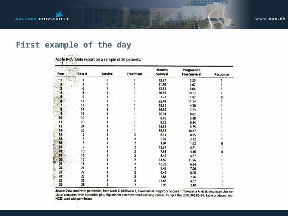
First example of the day

Problem
Do patients survive longer after treatment 1 than after treatment 2?Possible solutions:
• ANOVA on mean survival time?• ANOVA on median survival time?
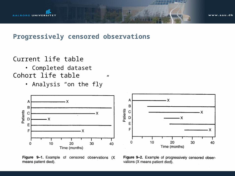
Progressively censored observations
Current life table• Completed dataset
Cohort life table• Analysis “on the fly”

Actuarial / life table anelysis
Treatment for lung cancer

Actuarial / life table anelysis
A sub-set of 13 patients undergoing the same treatment

Kaplan-Meier
Simple example with only 2 ”terminal-events”.
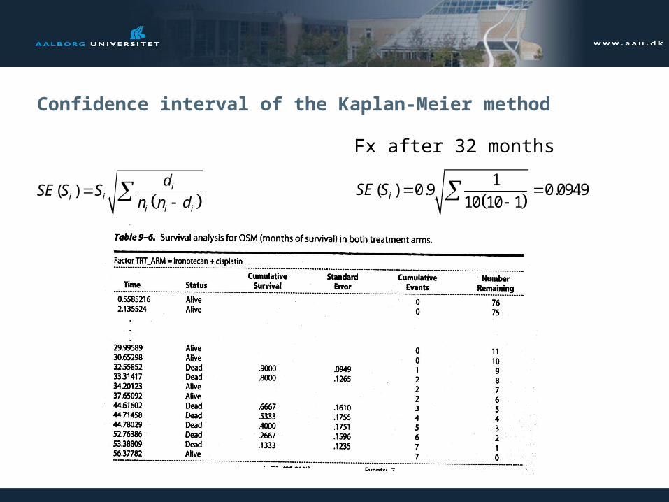
Confidence interval of the Kaplan-Meier method
Fx after 32 months
( ) ii i
i i i
dSE S S
n n d
1
( ) 0.9 0.094910 10 1iSE S

Confidence interval of the Kaplan-Meier method
• Survival plot for all data on treatment 1
• Are there differences between the treatments?

Comparing Two Survival Curves
• One could use the confidence intervals…
• But what if the confidence intervals are not overlapping only at some points?
• Logrank-stats
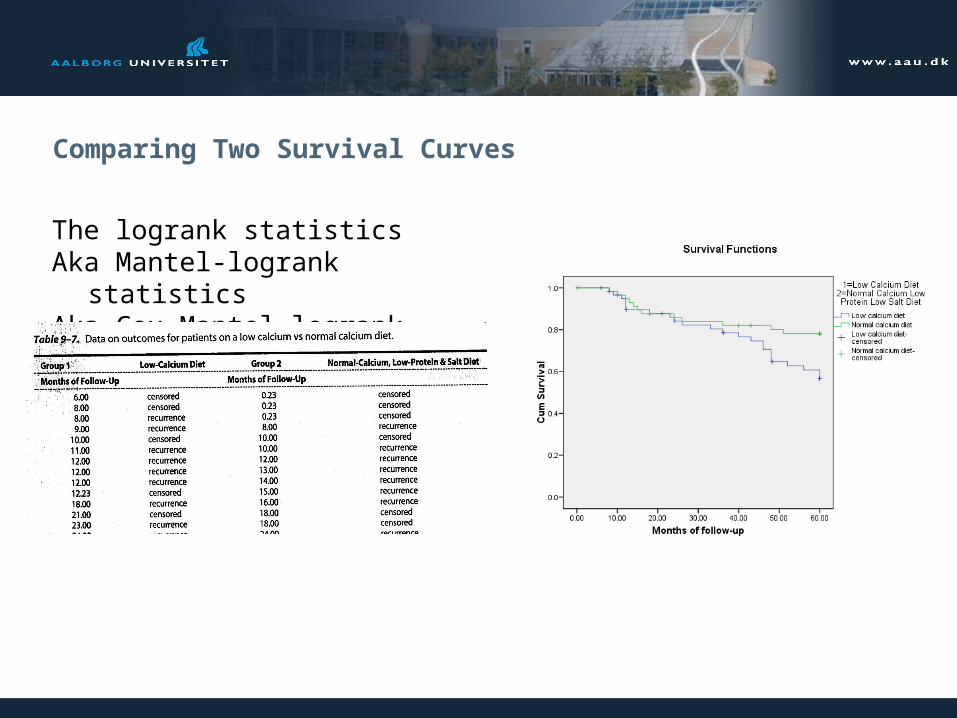
Comparing Two Survival Curves
The logrank statistics Aka Mantel-logrank statisticsAka Cox-Mantel-logrank statistics

Comparing Two Survival Curves
Five steps to the logrank statistics table1. Divide the data into intervals (eg. 10 months)2. Count the number of patients at risk in the groups and in
total 3. Count the number of terminal events in the groups and in
total4. Calculate the expected numbers of terminal events
e.g. (31-40) 44 in grp1 and 46 in grp2, 4 terminal events. expected terminal events 4x(44/90) and 4x(46/90)
5. Calculate the total

Comparing Two Survival Curves
Smells like Chi-Square statistics
2
2
all_treatments
O E
E
2 2
2 23 17.07 12 17.934.02
17.07 17.93
1df
0.05p

Comparing Two Survival Curves
1 1
2 2
23 17.07Hazard ratio 2.01
12 17.93
O E
O E