Embed Size (px)
Citation preview

Surface Plasmon Fluorescence Spectroscopy and
Microscopy Studies for Biomolecular Interaction Studies
Dissertation zur Erlangung des Grades
‘Doktor der Naturwissenschaft’
am Fachbereich Chemie und Pharmazie der
Johannes Gutenberg-Universität Mainz
vorgelegt von
Doene Demirgoez
aus Selimpasa, Istanbul-Turkey
Mainz, July, 2005

2
Dekan: Univ.-Prof. Dr. Peter Langguth
1. Berichterstatter: Prof. W. Knoll
2. Berichterstatter: Prof. Dr. W. Baumann
3. Berichterstatter: Prof. H. Decker
Tag der mündlichen Prüfung: 20, Juli 2005
Die vorliegende Arbeit wurde unter Betreuung von Herrn Prof. Dr. W. Knoll im
Zeitraum zwischen April 2002 bis Juli 2005 am Max-Planck-Institut für
Polymerforschung, Mainz angefertigt.

3
Contents
1 INTRODUCTION 5
1.1 The aim of the study 7
2 THEORETICAL BACKGROUND 8
2.1 Deoxyribo Nucleic Acid (DNA) 8 2.2 Peptide Nucleic Acids (PNAs): 10 2.3 Detection of DNA Hybridization on Surfaces 11 2.4 Genetically Modified Organism (GMO): 12 2.5 Detection of GMOs in food chain and EU regulations in GMO contained food labeling 12
2.5.1 DNA Based detection Methods: 13 2.5.1.1 Polymerase Chain Reaction (PCR): 13 2.5.1.2 Real Time PCR: 15 2.5.2 Protein Based Testing Methods: 16 2.5.2.1 Western Blot 16 2.5.2.2 ELISA (Enzyme Linked Immunosorbent Assay) 16 2.5.2.3 Lateral flow strip 17 2.5.2.4 The Nucleic acid sequence-based amplification (NASBA): 17
2.6 Microarrays 18 2.6.1 Making microarrays 18
2.7 Fluorescence 22 2.7.1 The Phenomena of the Fluorescence 22 2.7.2 Fluorescence Lifetime and Quantum Yield 23 2.7.3 Fluorescence Quenching 24 2.7.4 Photobleaching 25
2.8 Langmuir Adsorption 26 2.9 Evanescent Optics 29
2.9.2 Reflection and transmission of light 30 2.9.3 Surface Plasmon 32 2.9.4 Surface Plasmon with prism coupling 34 2.9.5 Optical Thickness 35
2.10 Surface Plasmon Fluorescence Spectroscopy (SPFS) 36 2.10.1 Fluorescence at the metal/dielectric interface 38
2.11 Surface Plasmon Microscopy (SPM)-Fluorescence Microscopy (SPFM) 39 2.11.1 Image Analysis 41
3 MATERIALS AND METHODS 44
3.1 Instrumental 44 3.1.1 Experimental Surface Plasmon Microscopy (SPM) and Surface Plas mon Fluorescence
Microscopy (SPFM) Set-up 47 3.2 Substrate and Metal Layer preparation 47
3.2.1 Self Assambled Monolayers (SAM) on gold 48 3.2.2 Binding of Streptavidin and preparation of the flow cell 50 3.2.3 Immobilization of the Catcher Probe onto the Substrate Surface 54 3.2.4 Hybridization reaction and Fluorescence Measurement 55 3.2.5 Surface Regeneration 61
3.3 Surface-Plasmon –Fluorescence Microscopy – A Novel Platform for Array Technology 62
3.3.1 Microarray preparation 62
4
3.3.1.1 Array Fabrication 62 3.3.1.2 Array Characterization 63 3.3.2 Hybridization between PNA-probe and oligonucleotides-target 63
RESULTS 64 4 PNA-DNA Hybridization Observed in Real-Time 64
4.1 Surface Plasmon Fluorescence Field-Enhanced Spectroscopy (SPFS) studies of PNA-DNA interaction on two dimensional (planar) surfaces 64
4.1.1 SPFS 4.1.2 Experimental 65 4.1.2.1 Fluorescence monitoring 65 4.1.3 Materials 66 4.1.4 Single kinetic measurements 69 4.1.5 Titration experiments 77 4.1.6 Global Analysis: 86
4.2 Surface Plasmon Fluorescence Microscopy (SPFM) studies of PNA-DNA interaction on microarrays 94
4.2.1 Aim 94 4.3 Conclusions 111
5 Genetically Modified Organism (GMO) detection in food chain by means of DNA-DNA and PNA-DNA Hybridization by Surface Plasmon Fluorescence Spectorcopy (SPFM) 113
5.1 DNA-DNA Hybridization on Biotin / Streptavidin Matrix 114 5.1.1 Aim 114
5.2 PNA-DNA Hybridization on SH-Streptavidin Matrix 125 5.2.1 Aim 125 5.2.2 Materials 125
5.3 CCD Saturation Test: 131 5.4 PNA-DNA Hybridization on Biotin thiol / Streptavidin Matrix 133
5.4.1 Array A 133 5.4.2 Array B 139
5.5 Conclusions 142
LIST OF FIGURES……………………………………………………………….144 LIST OF TABLES………………………………………………………………. ..152 APPENDIX A……………………………………………………………………...153
BIBLIOGRAPHY………………………………………………………………....154 ACKNOWLEDGEMENT LEBENSLAUF

5
1. INTRODUCTION
Biotechnology has enabled the modification of agricultural materials in a very
precise way. Crops have been modified through the insertion of new traits or the
inhibition of existing gene functions, named Genetically Modified Organism (GMO),
and resulted in improved tolerance of herbicide and/or increased resistance against
pests, viruses and fungi [Kuiper et al, 2002].
Seven millions farmers in 18 countries grew bioengineered crops on 167.2 million
acres in 2003, compared to 145 millions acres in 2002, according to ISAAA report. In
1996, which was the first year that genetically modified crops were commercially
available, about 4.3 million acres were under biotechnology cultivation [Kulkarni, 2004,
F.E.Ahmed, 2002].
Upon an increase of the population and lack in nutrition, some other countries like
South Africa and Brazil have also joined the GMO cultivated countries.
In Europe modified foods have not gained acceptance because of consumer suspicion
resulting from earlier food and environmental concerns, transparent regulatory
oversight, and mistrust in government bureaucracies. All these concern factors have
fuelled the debates about the environmental and public health issues of GMOs like
antibiotic resistance and gastrointestinal problems, destruction of agricultural
diversity, and potential gene flow to the other genes. Upon these developments, the
European Union regulations mandated labelling of GMOs containing food [EC, 1998,
2000]. Beside these reasons it is also important to allow the end consumers to make an
informed choice [Nature Biotech. News, 2001]. Hence, the regulations established a 1%
threshold for contamination of unmodified foods with GMO ingredients in early 2000.
A consequence of the declaration of a 1% threshold was the need to progress from
qualitative detection of alien DNA by using screening system to more complex
quantitative procedures.
Food, naturally, contains a range of different substances, such as fatty acids,
polysaccharides and lipids in addition to DNA and protein. Some of these substances
may negatively affect the assay techniques use to detect the GMOs. For example, the
presence of some plant polysaccharides can effectively inhibit polymerase chain
reaction (PCR) and in the absence of appropriate controls that result could be
interpreted as false negative.
6
Due to many other GMO varieties which are entering to the market or are in the
pipeline for approval, the necessity for a powerful detection method become a crucial
point. At this moment, microarrays seems to be holding the advantage of being able to
detect, identify and quantify the large numbers of GMO varieties in a sample in one
single assay.
By using microarrays, thousands of hybridization reactions can be screened
simultaneously by two-dimensional image analysis. However, detection systems for
microarrays require a highly sensitive and effective differentiation of signals from
noise. At present, the lack of sensitivity of the imaging systems brings the necessity of
using additiona l labelling techniques. Label based detection methods typically involve
the use of fluorescence, where the oligonucleotide targets are tagged with dyes that
are spectrally detectable. In fluorescence detection methods, the fluorescence signals
are quantified by photo multiplier tubes (PMTs) or charged-coupled devices (CCDs).
By measuring the fluorescence from labelled target molecules at different position on
a microarray, one can identify molecules and determine their relative abundance in a
sample. The most commonly used dyes are Cy5, Cy3 and AlexaFluor. These cyanine
dyes are suitable because they are sensitive, photo-stable, highly soluble in water and
exhibit low non-specific binding.
Fluorescence combined optical methods have enhanced sensitivity. One of the
well-established optical method for biological sensing is the surface plasmon
resonance (SPR) technique. It is a surface-sensitive optical method used to
characterize the layers on gold (Au) or noble metal thin films [Knoll, 1998]. These
measurements utilize the optical field enhancement that occurs at a metal/dielectric
interface when surface plasmons are generated. Surface plasmons are electromagnetic
waves that are excited by p-polarized light and propagate parallel to the Au surface.
The optical field decays exponentially from the surface of the metal and has a
maximum decay length of about 200nm. Within this region, the fluorophore can be
excited.
Beside GMO detection, DNA arrays hold the most promising way to transfer
complex biomolecular interaction in the interest of biomedical field. At the most basic
level, DNA arrays provide expression of whole genes in a cell on a single chip.
Therefore they also hold promise of transforming biomedical sciences by providing
new vistas of complex biological systems.

7
1.1 The aim of the study
Under the light of the information gained during the presented studies, two key
issues are addressed and solved.
1) what is the best strategy to design and built an interfacial architecture of a probe
oligonucletide layer either on a two dimensional surface or on an array platform;
2) what is the best detection method allowing for a sensitive monitoring of the
hybridisation events?
The study includes two parts:
1. Characterization of different PNAs on a 2D planar surface by means of
defining affinity constants using the very well established optical method
“Surface Plasmon Fluorescence Spectroscopy”(SPFS) and for the array
platform by “Surface Plasmon Fluorescence Microscopy” (SPFM),
determination of the sensitivity of these two techniques.
2. Detection of the existence and threshold value of alien DNA in food chain by
using DNA and PNA catcher probes on the array platform in real-time by
SPFM.

8
2. THEORETICAL BACKGROUND
2.1 Deoxyribo Nucleic Acid (DNA)
A DNA molecule in a organism contains all the genetic information necessary to
ensure the normal development of that organism. Therefore, they occupy a unique
position in the biochemical world.
The DNA monomers, which are referred to as nucleotides (nt), consist of three
subunits: a deoxyribose sugar, a base and a phosphate group [Saenger, 1983]. Linking of
the 3’ and 5’ OH of the sugar units via phosphodiester bonds creates a DNA strand.
The resulting ends of a DNA strand are designated as 3’ and 5’-terminus. The C1
atom of the ribose is attached to one of the four naturally occurring bases, the purines,
adenine and guanine, or the pyrimidines, cytosine and thymine. In single-stranded (ss)
DNA, the distance between two successive phosphates is about 0.7 nm. In a DNA
hybridization reaction, two complementary single strands of DNA become oriented in
an anti-parallel manner to form double-stranded (ds) DNA via Watson Crick base
pairing like the one depicted in Fig. 1 [Watson, 1953].
0,34 nm
2 nm
minorgroove
majorgroove
NN
O
OCH
3
HN
N
N
N
NH H
NN
O
N H
H
NN
N
N
O
NH
H
H
adeninethymine
cytosine
guanine
O
PO O
O
OBase
HHH
CH3
H
H
O
OBase
HHH
CH2
H
H
O
PO O
O
OBase
HHH
CH2
H
H
O
PO OO
1
23
4
5
5´ end
3' end
Figure 1: Schematic representation of the double helix (left) showing the minor and the major groove, a DNA single-strand illustrating the way the sugar units are linked via the H-bonding between specific Watson-Crick base pairs (right) and phosphodiester bridges (middle).

9
James Watson noted that hydrogen-bonded base pairs with the same overall
dimension could be formed only between A and T, and also G and C (figure 1). The
A-T base paired structure has two hydrogen bonds, whereas the G-C base pair has
three. The hydrogen bond pairs are formed between bases of opposing strands and can
only arise if the directional senses of the two interacting chains are opposite [Zubay et
al, 1995]. This structural information has been also proven by Francis Crick using X-
Ray diffraction pattern. The results were interpreted in terms of a helix composed of
two nucleotide strands. In this structure, the planes of the base pairs are perpendicular
to the helix axis and the distance between adjacent pairs along the helix axis is 3.4Å.
The structure repeats itself after 10 residues or once every 34 Å along the helix axis
[Zubay et al, 1995].
The stability of the DNA double helix structure depens on several factors. The
negatively charged phosphor groups are all located on the outer surface where they
have a minimum effect on each other. The repulsive electrostatic interactions
generated by these charged groups are often partly neutralized by the interaction with
cations such as Mg+2 [Tinland, 1997].
The process of separating the polynucleotide strands of a duplex nucleic acid
structure is called denaturation. Denaturation disrupts the secondary binding forces
that hold the strands together. These secondary binding forces are the hydrogen bonds
in between the base pairs of opposing strands and the stacking forces between the
planes of the adjacent base pairs. Individually these secondary forces are weak but
when they act together, they give a high stability to the DNA duplex in an aqueous
solution.
The melting temperature, Tm, of the DNA is sequence-dependent thermodynamic
stability of DNA in terms of nearest-neighbor (n-n) base pair interaction and defined
as the temperature at which 50% of the DNA becomes single stranded [Geoffrey, 1995]
The Tm is primarily determined by double stranded DNA (dsDNA) length, degree of
GC content, the higher the mole percentage of the G-C base pairs, higher the Tm is
since the G-C base pair contains three hydrogen bonds whereas the A-T base pair has
only two, and degree of the complementarity between strands.
Other factors present in the aqueous solution can also affect the stability of the
strand. For example, salt has a stabilizing effect on DNA strands by acting on the
repulsive electrostatic interactions between negatively charged phosphate groups of
the DNA. Salt ions shield the cahrges and therefore stabilizes the duplex structure.
10
2.2 Peptide Nucleic Acids (PNAs)
PNAs are nucleic acid analogs composed of neutral psuedopeptide/protein- like
backbone with regular or modified nucleobases [Nielsen et al, 1991].
In recent years, PNAs have become more popular in gene-targeted drug development
and molecular biology tools due to some advantages that PNA shows as compared to
the other analogues. One of the reason for this is the fact that PNA oligomers are
virtually resistant to degradation by nucleases, which insures the stability of the PNAs
in plasma and cell extracts [Nielsen, 2002].
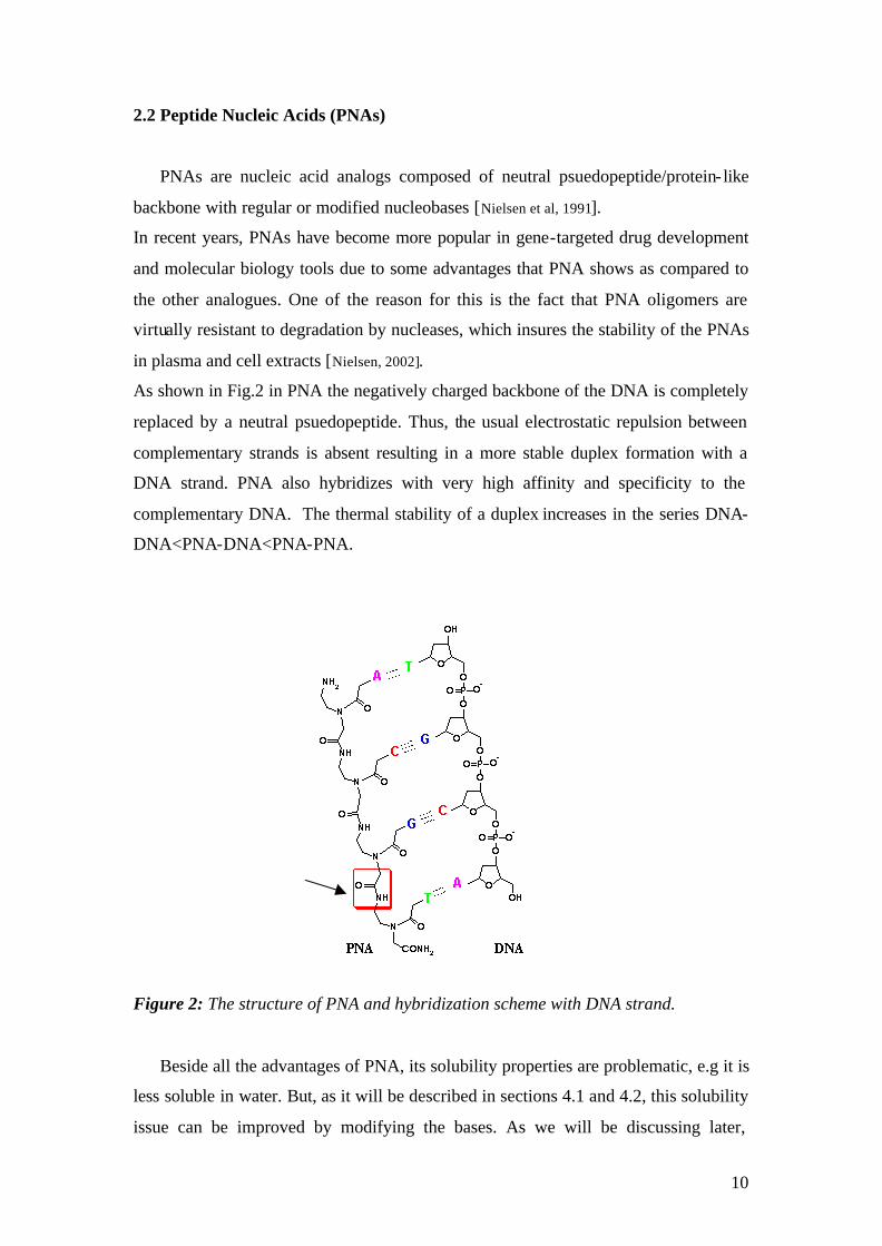
As shown in Fig.2 in PNA the negatively charged backbone of the DNA is completely
replaced by a neutral psuedopeptide. Thus, the usual electrostatic repulsion between
complementary strands is absent resulting in a more stable duplex formation with a
DNA strand. PNA also hybridizes with very high affinity and specificity to the
complementary DNA. The thermal stability of a duplex increases in the series DNA-
DNA<PNA-DNA<PNA-PNA.
Figure 2: The structure of PNA and hybridization scheme with DNA strand.
Beside all the advantages of PNA, its solubility properties are problematic, e.g it is
less soluble in water. But, as it will be described in sections 4.1 and 4.2, this solubility
issue can be improved by modifying the bases. As we will be discussing later,

11
modifications that have been done to increase the solubility have also increased the
affinity of the binding PNA to the complementary DNA strand.
2.3 Detection of DNA Hybridization on Surfaces
Biosensors are devices that combine a biological recognition element, which gives
selectivity, and a transducer, which provides sensitivity and converts the recognition
event into a measurable signal [Collings et al, 1997]. The biological recognition element
can be for example a single-stranded or double stranded either natural or synthetic
oligonucleotide [Tombelli et al, 2001].
The recognition event is a hybridization reaction between a surface immobilized
probe and a target. A sequence of bases forming the oligonucleotide on the sensor is
called the probe. It is complementary strand from solution is called target. The probes
are generally short oligonucleotides which are immobilized on a selected surface and
coupled to an optical, electrochemical, thermal or mass sensitive transducers whereas
targets are freely dissolved in solution.
Optical biosensors are sensitive to changes in the optical properties in a
solid/liquid interface upon any interaction between probe and target. This change
might result either in a refractive index change, luminescence or fluorescence.
Foremost important for any surface detection method is that only a specific adsorption
process of interest is measured while any other non-specific processes do not
contribute significantly to the final result. Optical biosensors offer several assets
among other biosensor types: (1) generally there is no need to label the molecules
being detected; (2) many important biological recognition takes place at surfaces; (3)
the signal/noise ratio is better and hence the sensitivity is higher and (4) they can be
used to monitor recognition processes in real time and in situ [Homolo, 2003].
The concept of detecting DNA hybridization on a surface has been widely
employed using various optical surface techniques including surface plasmon
spectroscopy [Kambhampati et al., 2001, Jordan et al., 1997 McDonnell, J. M. et al., 2001],
waveguide spectroscopy [Plowman, 1996], fibre optics evanescent wave spectroscopy
[Scheller et al., 2001] and quartz-crystal microbalance methods [Yun et al., 1998 and Qian et
al., 1998].

12
2.4 Genetically Modified Organism (GMO):
Genetically modified organisms are defined as living organisms whose genome
has been modified by the introduction of an exogenous gene, which is able to express
an additional protein that confers new characteristics [Mariotti et al., 2002].
The foreign DNA is usually inserted in a gene cassette consisting of an expression
promoter, a structural gene, which has an encoding region and an expression
terminator.
Considering GMO plants, a new gene can confer herbicide tolerance,
fertility/maturation modification or parasite, virus, fungi, drug or insect resistance.
The pesticide “Roundup” works by inhibiting an enzyme that is necessary for the
plant to synthesis certain aromatic aminoacids that are killing the plant. The targeted
enzyme is called 5-enolpyruvyl shikimate-3-phophate synthease (EPSP). The genetic
modification in Roundup Ready soybeans involves the incorporation of a bacterial
version of this enzyme into soybean plant to give a soybean protection against
Roundup [Minunni et al., 2001].
2.5 Detection of GMOs in food chain and EU regulations in GMO contained food
labeling
There are several issues concerning health and safety since GMOs are introduced
to the market. The general public concerns about the risk assessment of GMO
products because many GMO products are used as foods. Environmental concerns
derived from the result that GMO product effects on components of the ecosystem are
not easily observable in the short-term. Those are all because of the lack of knowledge
on the effects of many health-positive, intrinsic plant compounds on the following
issues [Kuiper et al, 2003].
• which compounds exert beneficial affects
• mechanisms of health promoting effects and of potential toxicity
• bioavailability of compound of interest
• matrix effects of on bioavailability and metabolism
• interaction between bio-active compound
• dose-response relationship of protective and adverse effects
• losses or modifications of compounds through food processing

13
Due to these facts, the detection of GMOs became socially and politically
important in many countries. Hence many countries have developed their own laws
controlling the marketing of GMOs [Kok et al, 2002]. While, for example, labelling is
not required in the US, in the EU it is mandatory. In the EU, the directive 90/220
regulates the approval and the release of the GMOs.
Raw material and processed products like foods derived from GM seeds might be
hold apart by testing for the presence of introduced DNA or by detecting expressed
novel proteins encoded by genetic material. Both qualitative and quantative methods
which give a yes/no answer are available [Tzu-Ming Pang, 1991].
Quantitative detection methods are needed for the enforcement of the labeling
threshold for GMOs in food ingredients. The labeling threshold is set to 1% in the
European Union and Switzerland and must be applied to all GMOs. Until now, four
different varieties of maize, insect-resistant Bt176 maize, Bt11 maize, Mon810 maize
and herbicide tolerant T25 maize are approved in the EU [Broadman et al,2002].
Some analytical methods are already available for GMOs detection, based on
detection of a) exogenous DNA and b) of proteins.
2.5.1 DNA Based detection Methods:
2.5.1.1 Polymerase Chain Reaction (PCR)
One method for the detection of the transgenic material in DNA is “the real time
Polymerase Chain Reaction (PCR)” approach.
PCR entails the enzymatic amplification of specific DNA sequences, target strand,
using two oligonucleotide primers that flank the DNA segment to be amplified and
give millions of the original copy (Fig.3).
A cycle consists of each set of the three steps as described below. The extension
products of one primer provide a template for the other primer in a subsequent cycle
so that each successive cycle essentially doubles the amount of DNA. This results in
the exponentially accumulation of the specific target fragment by approximately 2n,
where n is the number of the cycle. The specific target fragment is also referred to as
the “short product” and is defined as the region between the 5`ends of the extension
primers. Each primer is physically incorporated into one strand of the short product.
14
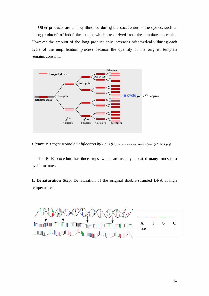
Other products are also synthesised during the succession of the cycles, such as
“long products” of indefinite length, which are derived from the template molecules.
However the amount of the long product only increases arithmetically during each
cycle of the amplification process because the quantity of the original template
remains constant.
Figure 3: Target strand amplification by PCR (http://allserv.rug.ac.be/~avierstr/pdf/PCR.pdf)
The PCR procedure has three steps, which are usually repeated many times in a
cyclic manner.
1. Denaturation Step: Denaturation of the original double-stranded DNA at high
temperatures
2n+1 copies n cycle
Target strand
A T G C bases
15
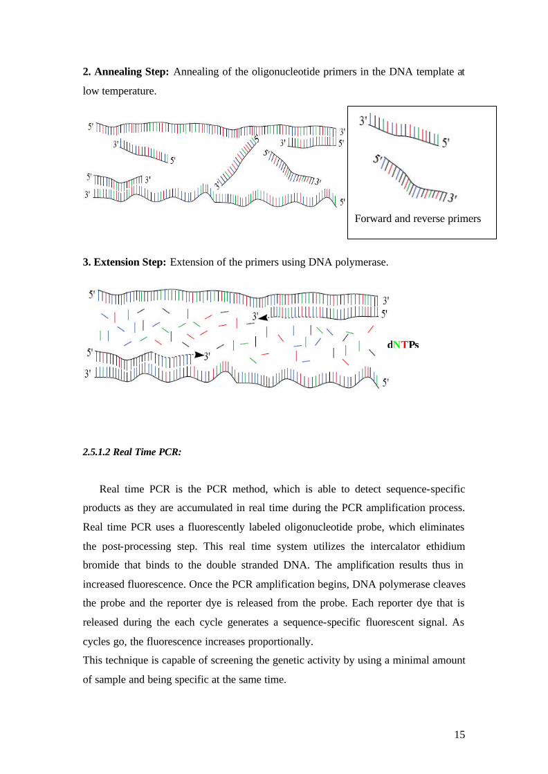
2. Annealing Step: Annealing of the oligonucleotide primers in the DNA template at
low temperature.
3. Extension Step: Extension of the primers using DNA polymerase.
2.5.1.2 Real Time PCR:
Real time PCR is the PCR method, which is able to detect sequence-specific
products as they are accumulated in real time during the PCR amplification process.
Real time PCR uses a fluorescently labeled oligonucleotide probe, which eliminates
the post-processing step. This real time system utilizes the intercalator ethidium
bromide that binds to the double stranded DNA. The amplification results thus in
increased fluorescence. Once the PCR amplification begins, DNA polymerase cleaves
the probe and the reporter dye is released from the probe. Each reporter dye that is
released during the each cycle generates a sequence-specific fluorescent signal. As
cycles go, the fluorescence increases proportionally.
This technique is capable of screening the genetic activity by using a minimal amount
of sample and being specific at the same time.
Forward and reverse primers
dNTPs

16
2.5.2 Protein Based Testing Methods:
Immunoassay technologies with antibodies are a good way for quantitative and
qualitative detection of many types of proteins in complex matrices when the target
analyte is known. Both a monoclonal antibody, which is highly specific, and a
polyclonal one, which is often more sensitive, can be used depending on the particular
application, time and cost. The detection limit of a protein immunoassay can predict
the presence of modified proteins in the range of 1% GMOs. Immunoassays with
antibodies attached to a solid support have been used in two formats:
1. a competitive assay in which the detector and analyte compete to bind with
capture antibodies.
2. two sided (double antibody sandwich) assay in which the analyte is a
sandwich in between the capture antibody and the detector antibody [Cochet et
al., 1998].
2.5.2.1 Western Blot
The Western blot is an highly sensitive, particularly useful method for soluble
proteins. It provides qualitative results for determining whether the sample contains a
target protein in the amount tha t exceeds the threshold limit or not. The samples that
will be assayed, are solubilized with detergents or reducing agents and separated by
Sodium Dodecyl Sulfate-polyacrylamide gel electrophoresis. Those components are
then transferred to a solid support such a nitrocellulose membrane and binding
immunoglobulin sites on the membrane are blocked by dried nonfat milk. Western
Blot analysis can only detect one protein in the mixture of any number of others.
However sensitivity of this method is highly dependent on the selected antibody’s
specificity to the corresponding protein.
2.5.2.2 ELISA (Enzyme Linked Immunosorbent Assay)
ELISA is a good testing method to estimate the amount of the target material in
ng/ml to pg/ml concentrations in solution. Based on the principle of antibody-antigen
interaction, it combines the specificity of antibodies with the sensitivity of the enzyme
assay systems.
17
Beside being used in clinical testing, it has also started to find a place in GMO
detection in recent years. Some companies like GeneScan and AgroGene use an
ELISA based method to quantify alien DNA in products.
In an ELISA test for genetically modified agricultural products, the biologically
engineered gene is isolated and antibodies are raised against specific surface
structures of this protein. If the protein is available in the sample, it is bound to the
walls of the test holder and react with tagged antibodies resulting in a change of colors
which can be detected by a fluorescence scanner.
2.5.2.3 Lateral flow strip
Lateral flow tests, or immunochromatographic strip tests (ICS are performed with
a visually detectable solid support (strip), to which basically any ligand can bind.
According to the type of the ligand molecule, e.g. dyed microspheres, qualitative
determination or semi quantitative detection might be performed.
Commercial test kits for Roundup Ready soybean genes are available from many
companies such as Strategic Diagnostic Inc., Naogen Corp., Enviroogix Inc. etc.
(www.usda.gov). However, according to a reviewed article in The International
Journal of Food Science and Technology, the ICS tests gave false negative results
more than 30% of the time for samples containing 0.5% and 1% GMO soybeans.
There are a number of technologies currently available that can be used to
overcome the disadvantages of those methods. For example, Surface Plasmon
Microscopy (SPM) and Spectroscopy (SPS), Surface Plasmon Fluorescence
Microscopy (SPFM), and Spectroscopy are currently available methods to observe
biomolecular interaction either in an array or on a surface in real time.
2.5.2.4 The Nucleic acid sequence-based amplification (NASBA):
The Nucleic acid sequence-based amplification (NASBA) technique amplifies an
RNA target molecule. One of the primers contains a T7 promoter, which allows for
the production of a RNA molecule after cDNA synthesis. There are some methods to
detect the antisense RNA molecules, among which FRET and molecular beacon
methods are the most suitable ones. A disadvantage of this type of technique is that
the test is based on the detection of RNA . It has the tendency to degrade easily and
18
therefore it’s only detectable in intact cell systems, which are also hard to work with.
Because of the varying expression level, the quantification of the GMO content with
this method is not straightforward.
2.6 Microarrays
Microarrays are comprised of large sets of nucleic acid probe sequences which are
immobilized in defined, addressable locations on the surface of a substrate.
Microarrays are capable of acquiring huge amounts of genetic information from
biological samples through single hybridization procedure.
In the late 1960s, Pardue and Gall [Pardue et al., 1969] and Jones and Robertson
[Jones et al., 1970] discovered a way of locating the position of specific sequences in the
nucleus or in chromosomes. They used hybridization reactions on a cell fixed to a
microscope slide. This method allowed DNA to take a part in duplex formation with
the probe that is being used to fix DNA spotted slides in one microarray method.
In the mid 1970s, recombinant DNA methods have been developed and the front of
discovering new genes had been opened [Grundstein and Hogness, 1975].
One attractive method for monitoring biomolecular interactions is high throughput
analysis and in this context, the microarray technique takes the most favourable place.
Microarrays have been used in genomic work, gene expression, protein screening and
the recently growing area of genetically modified organism (GMO) detection using
extremely limited amounts of biological samples.
Modern drug discovery efforts require the screening of millions of compounds in
a high throughput format before novel therapeutic moieties can be identified. The
same is true for all kinds of assays, which are perfo rmed in several hundreds of
thousands in certain disease categories.
2.6.1 Making microarrays
Printing is an easy and cheap way to produce a microarray among other surface
patterning techniques e.g, microcontact printing.
Printing of an array can be categorized according to following aspects: choice of
(1) the spotting system, (2) the surface chemistry for probe attachment, and (3) the
spotting solution.
19
(1) Spotting System
The choice of the spotting system is important for controlling the drop volume,
spot size and the homogeneity. A spotting device can either release the drops (ink-jet
spotter) or leave them as a result of a contact between pin and the surface (pin-tool
spotter)
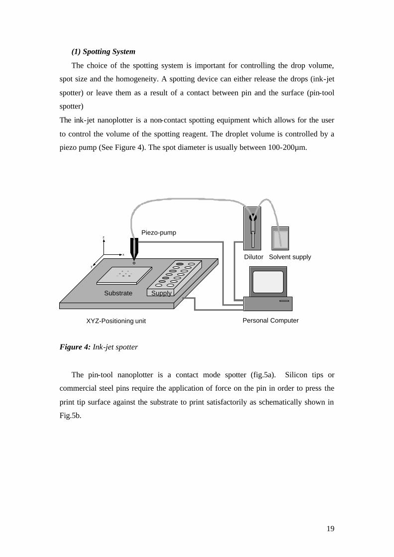
The ink-jet nanoplotter is a non-contact spotting equipment which allows for the user
to control the volume of the spotting reagent. The droplet volume is controlled by a
piezo pump (See Figure 4). The spot diameter is usually between 100-200µm.
x
y
z
Personal ComputerXYZ-Positioning unit
Dilutor Solvent supply
Substrate Supply
Piezo-pump
Figure 4: Ink-jet spotter
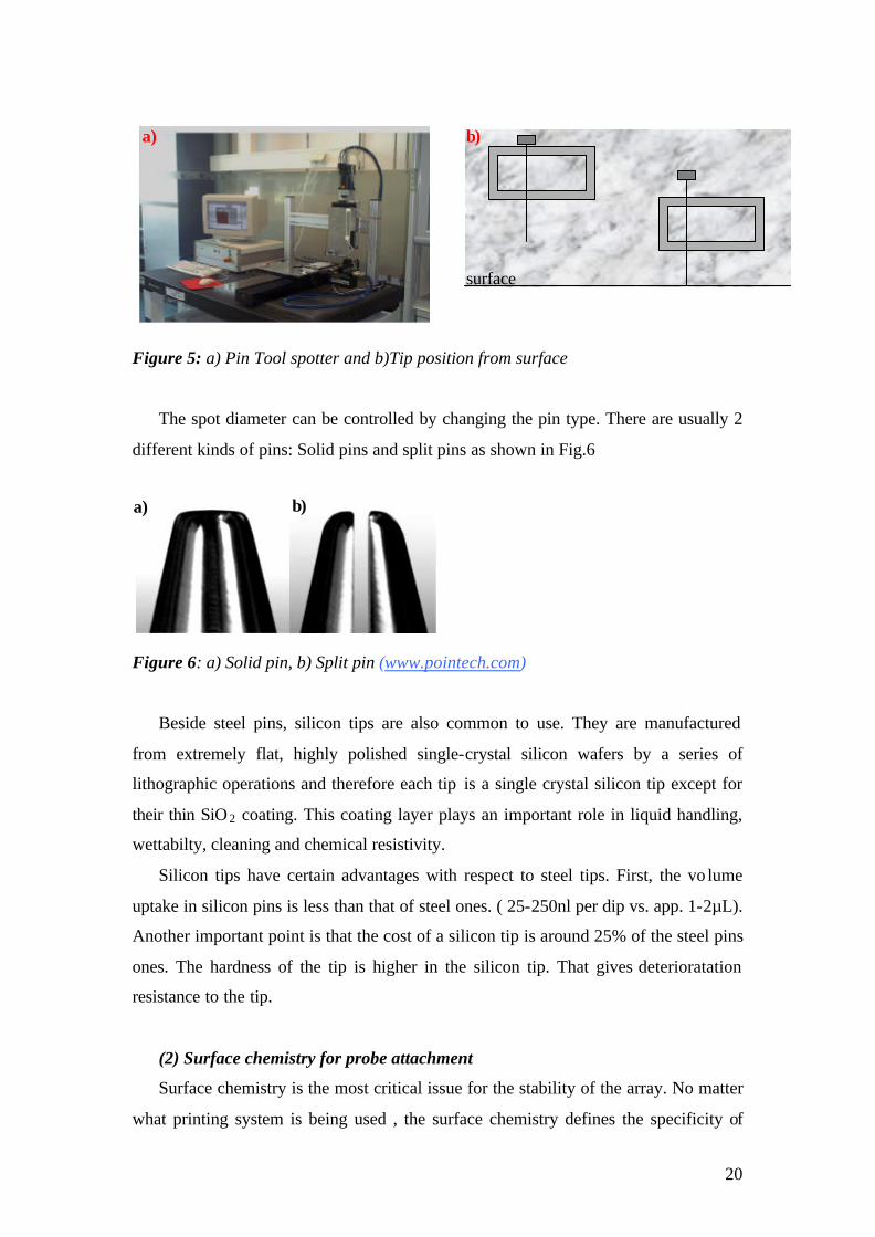
The pin-tool nanoplotter is a contact mode spotter (fig.5a). Silicon tips or
commercial steel pins require the application of force on the pin in order to press the
print tip surface against the substrate to print satisfactorily as schematically shown in
Fig.5b.
20
Figure 5: a) Pin Tool spotter and b)Tip position from surface
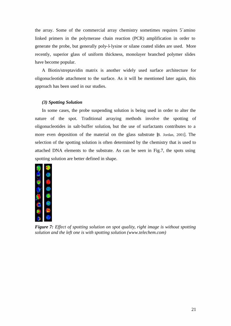
The spot diameter can be controlled by changing the pin type. There are usually 2
different kinds of pins: Solid pins and split pins as shown in Fig.6
Figure 6: a) Solid pin, b) Split pin (www.pointech.com)
Beside steel pins, silicon tips are also common to use. They are manufactured
from extremely flat, highly polished single-crystal silicon wafers by a series of
lithographic operations and therefore each tip is a single crystal silicon tip except for
their thin SiO 2 coating. This coating layer plays an important role in liquid handling,
wettabilty, cleaning and chemical resistivity.
Silicon tips have certain advantages with respect to steel tips. First, the vo lume
uptake in silicon pins is less than that of steel ones. ( 25-250nl per dip vs. app. 1-2µL).
Another important point is that the cost of a silicon tip is around 25% of the steel pins
ones. The hardness of the tip is higher in the silicon tip. That gives deterioratation
resistance to the tip.
(2) Surface chemistry for probe attachment
Surface chemistry is the most critical issue for the stability of the array. No matter
what printing system is being used , the surface chemistry defines the specificity of
a) b)
surface
a) b)
21
the array. Some of the commercial array chemistry sometimes requires 5´amino
linked primers in the polymerase chain reaction (PCR) amplification in order to
generate the probe, but generally poly- l- lysine or silane coated slides are used. More
recently, superior glass of uniform thickness, monolayer branched polymer slides
have become popular.
A Biotin/streptavidin matrix is another widely used surface architecture for
oligonucleotide attachment to the surface. As it will be mentioned later again, this
approach has been used in our studies.
(3) Spotting Solution
In some cases, the probe suspending solution is being used in order to alter the
nature of the spot. Traditional arraying methods involve the spotting of
oligonucleotides in salt-buffer solution, but the use of surfactants contributes to a
more even deposition of the material on the glass substrate [B. Jordan, 2001]. The
selection of the spotting solution is often determined by the chemistry that is used to
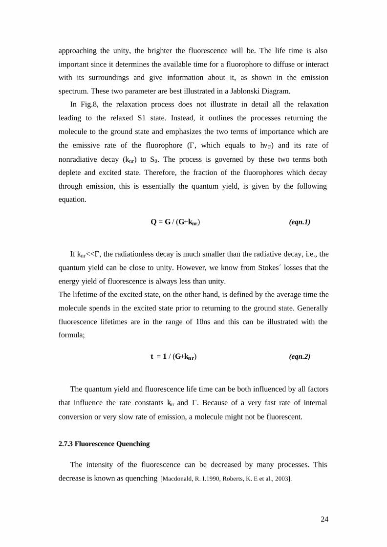
attached DNA elements to the substrate. As can be seen in Fig.7, the spots using
spotting solution are better defined in shape.
Figure 7: Effect of spotting solution on spot quality, right image is without spotting solution and the left one is with spotting solution (www.telechem.com)

22
2.7 Fluorescence
During the past years, the use of fluorescence techniques in biological sciences
has increased dramatically, especially for the observation of cell growth, clinical
chemistry and genetic analysis [Mary -Ann Mycek, 2003]. Because of that growing
interest, the instrumental part has been developed even though the basic fluorescence
principle is used. In this chapter, these basic principles of the fluorescence phenomena
will be described.
2.7.1 The Phenomena of the Fluorescence
The emission of light from a system is always a response to a process that brings
energy to the system. This response varies from biological response
(bioluminescence) to radioactive interaction. Luminescence is the emission of light
from any substance and involves any electronically excited states and can be divided
into two categories: Fluorescence and phosphorescence, depending on the nature of
the excited state.
Fluorescence is a phenomenon that describes emission of photons from molecules that
undergo a transition from an electronically excited state to the ground state [Lakowicz
J.R, 1983]. The processes that occur between the adsorption and emission of light are
illustrated by a Jablonski diagram [Mary-Ann Mycek, 2003].
Figure 8: Jablonski energy level diagram

23
The scheme in Fig.8 shows different electronic states, the eletronic ground state
designated as singlet (S0) and the first existed singlet state, S1. In each of these
electronic states, the molecule can exist in a number of vibrational levels, which are
populated according to the Boltzmann distribution law. The molecule exists in the
lowest vibrational state of the electronic ground state prior to photon absorption. In
the Jablonski diagram, the vertical lines indicate the nature of light absorption. After
absorption of the light, transitions occur within 10-15s. A fluorophore is usually
excited to higher vibrational level of S1 or S2 (not shown here). The absorption
spectrum therefore reveals information about the electronically excited states of the
molecule. With a few exceptions, molecules in condensed phases rapidly relax to the
lowest vibrational level S1. This process is called “internal conversion” and generally
occurs on a time scale of 10-12s. Since the fluorescence lifetime is typically near 10-8s,
this process is generally completed prior to emissions. Hence the fluorescence
emission generally results from thermally equilibrated excited state, which is the
lowest-energy vibrational state of S1. From there, the molecule can decay to different
vibrational levels of the state S0 by emitting light. This leads to fine structure of the
emission spectrum by which information can be gained about the electronic ground
state S0.
If a comparison is made between emission and absorption spectra, one can
observe that the energy of the emission is typically less than that of the absorption.
Hence, fluorescence occurs at lower energies or, in other words, at longer
wavelengths. This phenomena was first observed by Sir G.G. Stokes, it has been
called “Stokes´ shift”. This shift can be explained by considering the energy lost
between two process due to the rapid internal conversion in the excited states (S1 and
S2) and the subsequent decay of the fluorophore to higher vibrational levels of S0.
This shift is fundamental to the sensitivity of fluorescence techniques since it allows
the emitted photons to be isolated from excitation photons detected against a low
background.
2.7.2 Fluorescence Lifetime and Quantum Yield
The fluorescence lifetime and quantum yield are the two most important
parameters in a fluorescence process. The quantum yield is the number of emitted
photons relative to the number of absorbed photons. The higher the quantum yield is,
24
approaching the unity, the brighter the fluorescence will be. The life time is also
important since it determines the available time for a fluorophore to diffuse or interact
with its surroundings and give information about it, as shown in the emission
spectrum. These two parameter are best illustrated in a Jablonski Diagram.
In Fig.8, the relaxation process does not illustrate in detail all the relaxation
leading to the relaxed S1 state. Instead, it outlines the processes returning the
molecule to the ground state and emphasizes the two terms of importance which are
the emissive rate of the fluorophore (Γ, which equals to hνF) and its rate of
nonradiative decay (knr) to S0. The process is governed by these two terms both
deplete and excited state. Therefore, the fraction of the fluorophores which decay
through emission, this is essentially the quantum yield, is given by the following
equation.
If knr<<Γ, the radiationless decay is much smaller than the radiative decay, i.e., the
quantum yield can be close to unity. However, we know from Stokes´ losses that the
energy yield of fluorescence is always less than unity.
The lifetime of the excited state, on the other hand, is defined by the average time the
molecule spends in the excited state prior to returning to the ground state. Generally
fluorescence lifetimes are in the range of 10ns and this can be illustrated with the
formula;
The quantum yield and fluorescence life time can be both influenced by all factors
that influence the rate constants knr and Γ. Because of a very fast rate of internal
conversion or very slow rate of emission, a molecule might not be fluorescent.
2.7.3 Fluorescence Quenching
The intensity of the fluorescence can be decreased by many processes. This
decrease is known as quenching [Macdonald, R. I.1990, Roberts, K. E et al., 2003].
Q = Γ / (Γ+knr) (eqn.1)
τ = 1 / (Γ+knr) (eqn.2)
25
Quenching can be caused by mechanisms such as the physical interaction with
other molecules in solution while the fluorophore is in the excited state. In that case
the mechanism is called “collisional quenching” and the molecule “quencher”. In this
case, the fluorophore returns to the ground state during the diffusive encounter with
the quencher. The molecules are not chemically altered during the process. The
decrease in the fluorescence intensity due to collisional quenching is well described
by the Stern-Volmer equation:
The term K in this equation is the Stern-Volmer quenching constant, kq is the
bimolecular quenching constant, τ0 is the unquenched lifetime, and [Q] is the
quencher concentration. A wide variety of molecules, for example, oxygen, halogens,
amines and electron-deficient molecules like acrylamide can act as collisional
quenchers.
Beside collisional quenching, there are other ways to cause fluorescence
quenching. One of them is that fluorescent molecule can form a non-fluorescent
complex with the quencher. This process refers to a static quenching since it occurs in
the ground state and does not rely on molecular collisions or diffusion. Quenching
can also occur by other trivial mechanisms such as attenuation of incident light by the
fluorophore or other absorbing species.
2.7.4 Photobleaching
A typical fluorophore can undergo a finite number of excitation-relaxation cycles
prior to photochemical destruction. This process is often referred to as
photobleaching. For a photostable fluorophore, e.g. tetramethylrhodamin,
photobleaching occurs after about 105 cycles. In contrast, some molecules, like
fluorescein, photobleach very easily. Generally speaking, the photobleaching involves
the generation of reactive oxygen molecules, thus it is sometimes useful to introduce
antioxidants or to use anoxic conditions. On the other hand, the rate of the
photobleaching is often proportional to the intensity of illumination. Therefore, a
simple practical way to overcome this is to reduce the time or the intensity of the
excitation radiation.
F / F0= 1 + K[Q]=1+ kq τ0[Q] (eqn.3)
26
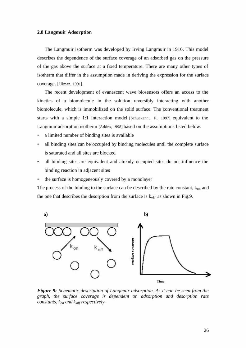
2.8 Langmuir Adsorption
The Langmuir isotherm was developed by Irving Langmuir in 1916. This model
describes the dependence of the surface coverage of an adsorbed gas on the pressure
of the gas above the surface at a fixed temperature. There are many other types of
isotherm that differ in the assumption made in deriving the expression for the surface
coverage. [Ulman, 1991].
The recent development of evanescent wave biosensors offers an access to the
kinetics of a biomolecule in the solution reversibly interacting with another
biomolecule, which is immobilized on the solid surface. The conventional treatment
starts with a simple 1:1 interaction model [Schuckannu, P., 1997] equivalent to the
Langmuir adsorption isotherm [Atkins, 1998] based on the assumptions listed below:
• a limited number of binding sites is available
• all binding sites can be occupied by bind ing molecules until the complete surface
is saturated and all sites are blocked
• all binding sites are equivalent and already occupied sites do not influence the
binding reaction in adjacent sites
• the surface is homogeneously covered by a monolayer
The process of the binding to the surface can be described by the rate constant, kon and
the one that describes the desorption from the surface is koff as shown in Fig.9.
Figure 9: Schematic description of Langmuir adsorption. As it can be seen from the graph, the surface coverage is dependent on adsorption and desorption rate constants, kon and k off respectively.
Time
a) b)
27
The adsorption mechanism can be described as an equilibrium between surface
bound molecules and molecules which are free in solution. The process of association
involves the binding of the analyte from solution onto the interface while the
dissociation process entails the detachment of bound analyte that then diffuse back
into solution. The resulting time dependent surface coverage, Θ, can be described by
the following expression;
Θ−Θ−=∂Θ∂
offon kCkt
)1(
in which c0 is the analyte concentration. One can see that the higher the analyte
concentration is, the faster the surface binding reaction is. On the other hand, the
desorption process has no relation with the analyte concentration and only depends on
the dissociation rate constant, koff, and the surface coverage. If we combine eqn.4 with
the initial equilibrium conditions, i.e., surface coverage, Θ=0 at t=0, we can derive the
following eqn.
The typical solution of this equation is given in fig.9-b, where the adsorption
process leads to the equilibration of the system at a certain surface coverage, which is
dependent on both rate constants. In the case of a real experiment the desorption
process can be followed separately by exchanging the analyte solution against pure
buffer, since the concentration c0 equals to zero and the first expression in eqn.5
becomes negligible. The rate constant koff can thus be derived by the consideration of
desorption alone with the simulation of experimental data following eqn 6.
)exp()( tkot off−Θ=Θ
where Θ0 is the initial surface coverage at the beginning of the desorption process. For
simplicity, it’s assumed that any re-binding of already rinsed off analyte is negligible.
In order to complete the experimental justification of the Langmuir isoterm, a
titration process can be performed. The titration process is the stepwise saturation of
Eqn. 4
Eqn.5
Eqn.6
)) )(exp( 1( tkkc offono +−−cokon cokon+koff
Θ(t)=

28
the surface with a known concentration of the analyte and allowing adsorption to
reach equilibrium. A new analyte solution with higher concentration is then injected
and allowed to equilibrate. This process is repeated until no more surface binding is
observed for the next analyte solution of higher concentration. Such titration
procedure allows each subsequent step to begin with a value of Θ0 higher than zero.
Solving eqn.6 with this initial conditions (Θ0=Θ at t=0 because of the higher surface
coverage already in place when adsorption is allowed to occur) leads to a solution of
the form;
The simplest relation of surface coverage to equilibrium constant K of the surface
reaction can be derived from eqn .4
This might be the most significant equation in the Langmuir model since it allows
direct calculation of the general equilibrium constant K from two simple experimental
parameter like analyte concentration and surface coverage. For the fluorescence
experiment, the surface coverage Θ is determined by scaling the detected signal
intensity against the theoretical maximum intensity obtained at total surface
saturation.
In reality, some limitations of the model have to be taken into account. The
surface coverage is mass transport limited if the analyte concentration is too low,
analyte molecules are too small or the lateral deposition density is too low. This case
is usually seen in titration measurements where the surface is started to be “decorated”
with the target molecule from very low concentration. In the fluorescence
measurement, the exchange rate between bound species and free species can bring
upon large influence in the measured signal due to detrimental effects of the photo-
bleaching and the possibility of recombination with the washed away molecule is also
not avoidable.
Eqn.7
Eqn.8
Θ(t)= ) (exp( tkkon c off o +−cokon
cokon+koff Θo
cokon
cokon+koff )
Θ= coK 1+ coK

29
2.9 Evanescent Optics
Because of the fast progress in sensor technology, the need of high sensitivity and
specificity has become a crucial issue. One way to fulfill that requirement is the
combination of sensors based upon Surface Plasmon Resonance Spectroscopy (SPR)
[Knoll, 1997]. These sensors are generally able to detect changes in refractive index
down to ∆n/n= 10-5 with a time resolution in the order of seconds [Jung et al, 1998].
SPR methods are surface sensitive techniques that employ the enhancement of the
optical fields that occur at metal like Au, Ag, Al, Cu etc. surfaces if surface plasmon
polaritons (SPPs) are created at the metal/dielectric interface.
2.9.1 Evanescent Light
The simplest case of the existence of an evanescent wave is the total internal
reflection of a plane electromagnetic wave at the base of a glass prism, with an index
of refraction n1, in contact with an optically less dense medium like air, n2 (n1>n2),
shown in Fig.10 [Knoll, 1991].
Figure 10: The basic configuration for evanescent optics
The relation between the reflected light intensity and angle of incidence, Θ, is
governed by Snell’s Law (eqn 9).
1211 sinsin θθ ′⋅=⋅ nn Eqn.9
n1 n2
Glass Prism
Light of incidence reflected light
Evanecent Field
Θ
ϕ

30
Upon the increase of the incidence angle θ1 in Fig.11, one finds that transmission
angle θ2 is increased until the maximum value of θ2= 90° is reached. Since sin90°= 1,
the Snell eqn. turns to eqn9 and then θ1 is called Critical Angle θc which is given by:
sinθc = n2/n1
At the same time, the intensity of reflected light increases to the maximum, while
the intensity of transmitted light is reduced until it vanishes at 90°. This particular
angle of incidence is referred to as the critical angle. Upon further increase of θ1, the
reflection coefficient remains 1, indicating total internal reflection (TIR). The TIR
regime is characterized by the existence of a plane wave travelling along the interface.
This wave exhibits an electrical field component that decays exponentially in z-
direction. The penetration depth, d, of the evanescent field is in the range of the
wavelength λ that is used.
θ1
Hy
θ1'
θ2
Ei ki
Hy
Er
kr
Et kt
Hy
x
z
n1
n2
reflectiontransmission
incidence
Figure 11: Schematic representation of reflected and transmitted P-polarized light at the interface between two optically different media
2.9.2 Reflection and transmission of light
Imagine a system like the one in fig.11, an interface in the xy-plane between two
media with optical properties described by their refractive indices n1 and n2. Coming
from medium 1, monochromatic polarized light passes through the medium.
Depending on the angle of incidence θ1 and the optical constants of the materials, a
certain part of the light will be reflected and transmitted into the adjacent optical
medium with the sum of the energies of these two light waves being equal to that of
the original wave.
Eqn. 10
31
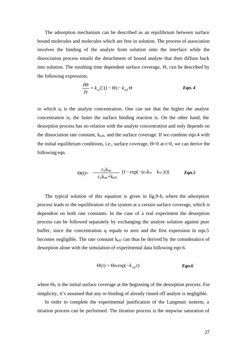
Since propagating light consists of a transverse electric and magnetic field, the
magnetic, Hx,y,z, and electric field components, Ex,y,z, can have different orientations
parallel or perpendicular to the surface. Two modes of polarization can be
distinguished for a wave propagating in the xy-plane:
Transversal magnetic polarization (TM or p-polarized light) with
0EHH yzx ===
and the non-vanishing components Ex, Ez and Hy. The electric field has a component
Ez that oscillates in a plane perpendicular to the xy-plane.
Transversal electric polarization (TE or s-polarized light) with
0HEE yzx ===
and the non-vanishing components Ey, Hx, Hz. Here, the electric field only has a field
component that oscillates in parallel to the xy-plane.
Below the critical angle for total internal reflection, the reflection differs slightly
for s- and p-polarized light. In the following considerations, we will focus on the TM
mode since only this mode is able to induce a surface charge density along the z-
direction, which is the pre-requisite for SP excitation. According to the reflection law,
the angle of incidence θ1 equals the angle upon which reflection occurs at 1θ′ . The
transmitted ray is diffracted towards the surface normal according to Snell’s law
(Eqn.9) with n1> n2. Monitoring the reflection R as a function of the angle of
incidence yields the reflection spectrum (with R=Ir/I0, where Ir is the intensity of the
reflected and I0 the intensity of the excitation light, respectively). It should be noted
that the intensity always corresponds to the square of the electric field, 2
E . The
spectrum can be theoretically predicted using a transfer matrix algorithm [Raether,
1988].
The electric field distribut ion in the immediate vicinity of the interface indicates
that, when TIR occurs above the critical angle, Θc, the light intensity does not fall
sharply to zero in air, in other words, the light intensity does not vanish completely.
Instead, a harmonic wave with an exponentially decaying amplitute perpendicular to

32
the interface is found to be traveling parallel to the surface. Such type of wave is
known as an evanescent wave [Deri F. et al, 1985] and its depth of penetration with
respect to the interface l is defined by the equation below.
2.9.3 Surface Plasmon
Plasmon Surface Polaritons (PSPs) are surface electromagnetic modes that travel
along a metal-dielectric interface as bound non-radiative waves, their field amplitudes
decaying exponentially perpendicular to the interface [Rather,1988]. They are created by
coupling energy from photons into oscillation modes of density at the metal/dielectric
interface (Fig.13-a) and formed from light waves Its electric field vectors or wave
vectors are oriented parallel to the plane of incidence. PSPs also have propagation
vectors or wavevectors, ksp, that lie in the plane of metal surface.
The dispersion relation (i.e. the energy-momentum relation) for SPs at a metal
(εm)/ dielectric (εd) interface is given by:
md
mdxx c
kikkspεε
εεω+
=′′+′=
where ω is the frequency of light, c is the speed of light, ksp is the wavevector of the
photon and εm and εd are the dielectric constant of the metal and dielectric which is
often air or water.
Since εm is complex, the wave vector kx has to be complex, too, where k?x
represents the damping part of the SP. Consequently, SPs exhibit a finite propagation
length L, given by Lx=1/k?x. The propagation length limits the lateral resolution of SP-
based microscopical methods. In a typical experiment at a gold/dielectric interfaces
and an excitation wavelength of 630 nm, the lateral resolution will be about 5 µm.
Excitation of the surface plasmon is possible either by electrons or by photons.
The previously discussed dispersion relation (eqn.12) has shown that the resonant
Eqn.11
Eqn.12

33
excitation cannot be realized by using free photons. The dispersion of free photons is
described by the light line:
ddphd
ccwithkc
ε=⋅=ω
Relevant for the excitation of SPs is only the projection of the wave vector k in x-
direction. For the simple reflection of a photon with the energy Lωh (fig.13-a) the
magnitude of the x-component, θ= sinkk phxph, , can be varied by changing the angle
of incidence, θ. kph,x vanishes for perpendicular incidence of light, while it is
maximized for large angles of incidence.
ω max
ω L
θ 0 θ
1
ω = c d k
SP1
SP2
1 2 3
A B
ω = c p k
Figure 12: Dispersion relation for A) free photons in a dielectric, B) free photons propagating in a coupling prism, SP1) surface plasmons at a metal/dielectric interface and SP2) surface plasmons after adsorption of an additional dielectric layer [Liebermann, 1999].
A graphical representation of the dispersion of free photons and SP modes is given in Fig.12. The dispersion of photons in the bulk is given as a straight line (A). The SP dispersion curve (SP1) approaches a maximum angular frequency that is attributed to
the plasma frequency of the employed metal. Increasing the angle θ from 0° to the grazing angle, tunes the curve from point 0 to point 1 (dark gray area). Because of the asymptotically approach of surface plasmon dispersion curve, SP1, to the line A at very low energies, the momentum matching conditions for resonant surface plasmon excitation cannot be met which means that coupling of the modes is not possible by
Eqn.13

34
changing the angle of incidence alone. Therefore, a way must be found to increase the momentum of light.
θ
prism
metal
dielectric
b
z
xmetal
dielectrickph,x
kpsp
θ
a
kph
Figure 13: a) Reflection geometry for photons with a momentum kph at a metal/dielectric interface. The angle of incidence θ determines the absolute value of the momentum in z-direction, kph, x, that is relevant for surface plasmon excitation. b) Kretschmann configuration for momentum matching via prism coupling.
2.9.4 Surface Plasmon with prism coupling
A common way to increase the momentum of light is a method based on prism
coupling. Using this method, the photons are not coupled directly to the
metal/dielectric interface but via the evanescent tail of light upon total internal
reflection at the base of a high refractive index prism (εp > εd) [Otto,A.Z, 1968,]. Line B
in Fig.12 describes the increased momentum of photons travelling through a high
index prism. By choosing the appropriate angle of incidence (point 2), resonant
coupling between the evanescent photons (B) and the surface plasmons (SP1) can be
achieved. After adsorption of a dielectric film (SP2) the resonance occurs at an angle
corresponding to point 3. The illustration of a prism coupling experimental set-up
known as the Kretschmann configuration is shown in Figure 13-b.
The geometry experimentally used in the present work, is the Kretschmann
configuration [Kretchmann E, 1968]. As depicted in Fig.13-b, a high index prism is
coated with a thin gold layer (~55 nm) adjacent to a lower index dielectric. We have
to note that the excitation of the PSPs requires efficient coupling between the metal
and the prism. Monochromatic p-polarized laser light is reflected at the base of the
prism under an angle of incidence larger than the critical angle. The evanescent field
resulting from total internal reflection overlaps with the surface plasmon mode and
resonance is achieved by tuning the angle of inc idence. If one monitors the intensity
detector
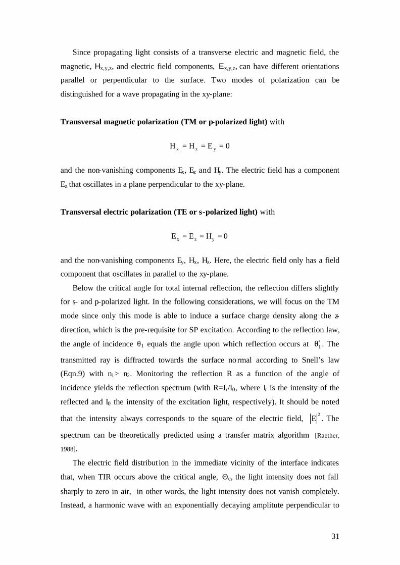
35
of the reflected light while sweeping through a range of angles, plasmon resonance
shows up as a sharp dip in the reflectivity spectrum at the resonance angle, as seen in
fig.14.
Figure 14: As it was described in the text above, resonant coupling is observed as a very pronounced drop in angular scan of the reflected light intensity at θR. θc is the critical angle for Total Internal Reflection (TIR).
It is also important to note that the finite thickness of the metal layer does affect
the dispersion behavior of the surface plasmon modes. In addition to the intrinsic
dissipation of energy in the metal itself, the coupling of some of the light through the
thin metal/prism interface creates another channel of radiative loss for surface
plasmon which will be discussed in more detailed in section 2.10.1.
2.9.5 Optical Thickness
As illustrated in Fig.12, the dispersion relation of SPs changes when a thin layer
of metal is deposited onto prism, effectively shifting the momentum-matching process
(from curve SP1 to SP2) and thus the incident angle at which surface plasmon
resonance occurs. Further deposition of metal layers or dielectric layer with different
dielectric constants will continue to shift the resonance angle (i.e. Fig.15). This is
largely due to increase of the overall refractive index detected by the evanescent
plasmon field. Consequently, the dispersion relation is shifted towards larger wave
vectors, kp2= kp1+∆k. In this expression kp2 and kp1 are wave vectors of the system
before and after the adsorption, and that ∆k is largely influenced by the refractive
index and the thickness of the layer absorbed. Such sensitivity to optical thickness is
Angular Scan Angle (θ)
Ref
lect
ivity
, R
36
one of the most fundamental and significant features of surface plasmon resonance
spectroscopy.
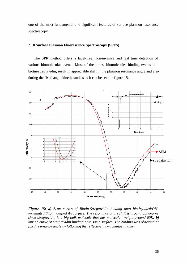
2.10 Surface Plasmon Fluorescence Spectroscopy (SPFS)
The SPR method offers a label- free, non-invasive and real time detection of
various biomolecular events. Most of the times, biomolecules binding events like
biotin-streptavidin, result in appreciable shift in the plasmon resonance angle and also
during the fixed angle kinetic studies as it can be seen in figure 15.
Figure 15: a) Scan curves of Biotin-Streptavidin binding onto biotinylated/OH-terminated thiol modified Au surface. The resonance angle shift is around 0.5 degree since streptavidin is a big bulk molecule that has molecular weight around 60K. b) kinetic curve of streptavidin binding onto same surface. The binding was observed at fixed resonance angle by following the reflective index change in time.
46 48 50 52 54 56 58 60 62 64 66Theta [°]
0
10
20
30
40
50
60
70
80
90
R [%
]
Scan-Messung
-5 0 5 10 15 20 25 30 35 40Zeit [min]
30
32
34
36
38
40
42
44
R [
%]
Kinetik-Messung
5 7 . 0 5 7 . 5 58.0 5 8 . 5 59.0 5 9 . 5 6 0 . 0 60.5 6 1 . 0
Theta [°]
2
4
6
8
10
12
14
16
R [%
]
Scan-Messung
a b
Ref
lect
ivit
y %
Scan angle (θ)
Time (min)
Ref
lect
ivit
y, R
rinsing
strepatavidin
SEM
37
Problems, however, arise if low molecular weight molecules, like short chain
DNA molecule or pharmaceutical drugs are involved in binding or if the packing
density of the film is very small. For such cases, the resonance angle shifts are very
small and SPR is no longer sensitive enough to monitor these binding events or
interactions accurately. Under such circumstances, there is a need to incorporate
certain signal amplification schemes that can be used in combination with SPR to
monitor all these interfacial interactions. Fluorescence tagging of molecules can lead
to amplification in the detected signal and thus offers an interesting way of monitoring
these low resonance shift events [Knoll, 1985].
The surface plasmon evanescent field can be used to excite the fluorescent dye
molecules. But only those chromophores lying within the vicinity of the interface are
excited. The emitted fluorescence is strongly dependent on the intensity of the optical
evanescent field at a given wavelength and also the probability of the radiative decay
of the chromophore from its excited state to the ground state. The optical excitation of
the fluorophores follows the evanescent field and since the evanescent field is
maximum near the resonance angle, a characteristic increase in the fluorescence
signal is observed.
Although the fluorescence coup ling with normal SPR results in an enhanced
sensitivity, the detected signal is a strong function of the plasmon electromagnetic
field. Any external stimuli, which causes a change in the plasmon field will be
directly affecting the fluorescence excitation. This effect can be seen if the refractive
index of the dielectric medium in contact with the metal changes under the influence
of temperature, pressure and the structure of the solvent and the plasmon
electromagnetic field is also altered. If the plasmon field changes, the fluorescence
excitation level also changes and leads to different fluorescent emission. Thus, if the
experimental set-up is designed, those special cases should be taken into account.
Another important point is that the SPFS technique requires the labeling of the
biomolecules. That means, every time one labels a biomolecule there is a high
probability of secondary effects introduced bye the labeling of the biomolecule.
In spite of the limitations that have been mentioned above, the SPFS technique
offers a way to observe various biomolecular interactions which can not be monitored
by using normal SPR. Since this detection technique is highly sensitive, it is possible
to carry out the experiment with a smaller amount of the material. That will help to
reduce the cost in the case of expensive materials. As it will be described in the

38
following sections, the fluorescence microscope, multi-spot detection of various
interactions can be also monitored simultaneously leading to high throughput analysis.
2.10.1 Fluorescence at the metal/dielectric interface
The fluorescence emission from the chromophores is strongly dependent upon the
distance from the metal surface. Fig.16 illustrates the distance dependence of the
chromophore to the metal surface [Barnes, W. L., 1998 Knobloch, H et al., 1993]: The ones
that are close to the metal surface are quenched and most of the excited state energy is
dissipated as heat. For the chromophores lying at intermediate distances from the
metal surface, some of their energies can be used in back couple to a surface plasmon
mode. And as a last case, at sufficient separation distances (>20 nm), free emission of
the dyes dominates. However, the fluorescence yield cannot be directly obtained
unless two effects are considered. Firstly, the fluorescence emission oscillates as the
distance increases, since the metal reflects the fluorescence field and introduces light
interference. Secondly, the excitation source, i.e., the evanescent field weakens as the
distance increases..
Dipole-to-dipole coupling Surface plasmon Free emission
prism
metal
dye
dielectric
Figure 16: Schematic drawing of a fluorophore positioned close to a metal/dielectric interface. Different fluorescence decay channels take place at different fluorophore/metal separation distances
This distance dependence of fluorescence emission is described by the Förster
equation;
39
140d
dd
1II
−
∞
+= eqn.14
where ∞I denotes the fluorescence intensity at infinite separation distance in the
absence of a metal surface, Id is the observed fluorescence intensity at a distance d
from the surface, d0 is the so called Förster radius that corresponds to the distance at
which the fluorescence is decreased to the 50 % level. This radius ranges typically
between 5 and 10 nm. Since the quenching effects can influence the quantitave
description of various interactions, it is really important to carefully design the
supramolecular architecture. This is the case in our working system, Streptavidin-
biotin system, where the thickness of the architecture is around 7-8nm, which is in the
quenching regime of the metal substrate.
In order to calculate a theoretical quenching profile for the present SPFS system,
one has to consider the probability for fluorescence emission in a) all directions b)
towards the photodiode on the backside of the prism and c) towards the gold surface,
where coupling of the fluorescence light to surface plasmons is possible.
2.11 Surface Plasmon Microscopy (SPM)-Fluorescence Microscopy (SPFM)
SPM and SPFM are imaging detection methods based on evanescent field optics
that allow for observation of oligonucleotide hbyridization in real time. These
methods offer both label and label- free detection modes, and as a result are useful
when dealing with delicate molecules where a label might significantly alter the
properties of any biomolecular interaction [Kambhampati D., 2004].
Surface plasmon microscopy, or SPM, has also been developed for spatially-resolved
DNA sensing, which can directly meet the needs in reading DNA or biomolecule
microarrays. This imaging technique is especially useful for the imaging of low-
contrast samples. SPM allows for the imaging of such systems without any addition of
fluorescent dyes, which is generally used to enhance discrimination (SPFM)
[Rothenhäusler et al., 1988].
The same theoretical principles of SPR are also valid for the microscopy. That
means any PSP spectrometer can be easily converted to a microscope by simply

40
adding a lens to the detection side and monitoring the obtained image on a screen or
with the help of CCD camera as shown in Fig.17.
´
Figure 17: Schematic representation of SPM & SPFM set-up (from Rothenhäusler et al., 488, 1988, Nature).
The sensitivity issue is important in microscopy as is the lateral resolution. The
lateral resolution in SPM is in the 1µm range. Even though we have to deal with
resonance contrast in SPM, this technique gives higher sensitivity than the other
microscopy techniques resolving 10nm thickness; since the detection scheme contains
plane-wave optical components, SPM is limited by diffraction. As it was explained in
previous sections, PSPs are propagating modes [Rather, 1988] which are strongly
damped in their propagation direction due to intrinsic dissipation and radiative
damping. A quantitative measure of how far a PSP mode travels is the propagation
length Lx is directly related to the imaginary part of the complex PSP wavevector, kix,
by Lx=(2kix)-1. If radiative damping can be neglected, Lx which is defined by the
complex dielectric function of the metal. Hence, Lx is the wavelength-dependent
higher spatial resolution in SPM, which is achieved with only lossy PSP modes.
CCD (SPFM)
Lens
Array
Prism
Lens
CCD (SPM)
Cr/Au coating
laser
41
In the case of SPFM, the resulting fluorescence emission is detected by a highly
sensitive CCD camera in the microscopic mode [Zizlsperger et a1 1998, Liebermann et
al,2003] which can be used then to observe the oligonucleotide hybridization process.
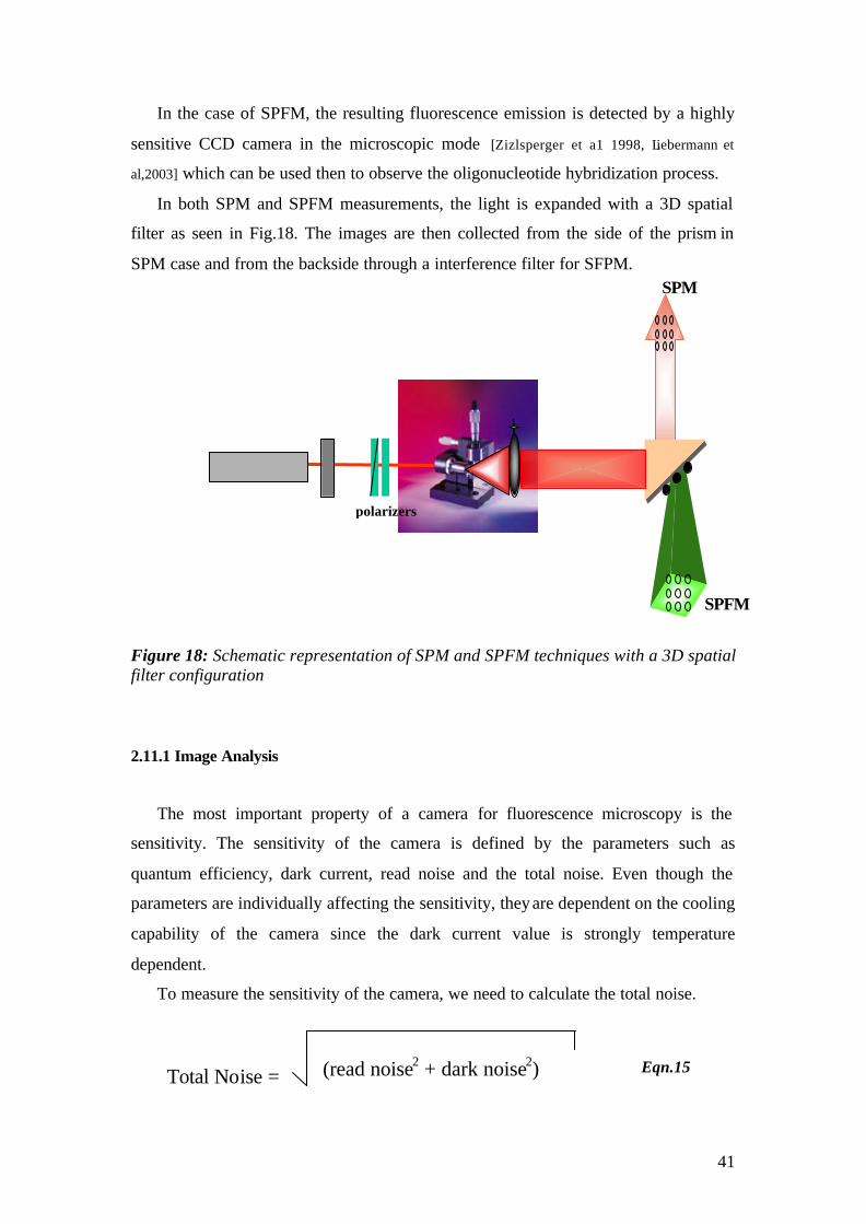
In both SPM and SPFM measurements, the light is expanded with a 3D spatial
filter as seen in Fig.18. The images are then collected from the side of the prism in
SPM case and from the backside through a interference filter for SFPM.
Figure 18: Schematic representation of SPM and SPFM techniques with a 3D spatial filter configuration
2.11.1 Image Analysis
The most important property of a camera for fluorescence microscopy is the
sensitivity. The sensitivity of the camera is defined by the parameters such as
quantum efficiency, dark current, read noise and the total noise. Even though the
parameters are individually affecting the sensitivity, they are dependent on the cooling
capability of the camera since the dark current value is strongly temperature
dependent.
To measure the sensitivity of the camera, we need to calculate the total noise.
SPFM
SPM
polarizers
Total Noise = (read noise2 + dark noise2) Eqn.15

42
Dark current is the charge that is thermally generated or in other word, it is the
charge accumulated within a pixel, in the absence of light. Dark current describes the
rate of generation of thermal electrons in a given CCD camera. High-performance
CCD camera systems reduce the dark noise by cooling the CCD with either
thermoelectric coolers (TECs), liquid nitrogen (LN2) or cryogenics camera
refrigeration during camera operation. For example dark current of a CooledSNAP
CCD camera is 5 e-/p/s at normal operating temperature while that value is 0.05 e-/p/s
at -30 °C. If these values are inserted in the equation to calculate the total noise for
normal operating temperature system, the value of the dark noise is increased and then
the total noise and as a result sensitivity decreases. For long exposure times, cooling
becomes very important. Especially for the observation of the kinetic binding of DNA
chains, a long term observation is needed to get reproducible association and
dissociation data.
Quantum efficiency is the measure of the effectiveness by which an imager
produces electronic charge from incident photons. Especially this is an important
property to perform low-light- level imaging. A good cooled CCD has a quantum
efficiency around 40-45%. Beside that, the pixel size defines the resolution.
Resolution of a CCD is a measure of how fine a detail can be detected in terms of
pixel.
When an image is quantified, the gray value is the main output to measure.
Average Gray value is the average of the pixel grayscale values contained in the
object.
(dark current) x (integration time)
Dark Noise = Eqn.16
Eqn.17

43
Total Gray Value is the sum of the grayscale values for all pixels contained in the
object. Also referred to as Integrated Gray Value.
Another function for the image analysis is the intensity profile of the image.
Intensity Profile is a function in the image analysis program MetaMorph which
creates an image that represents a source image's intensity levels as heights in a "3-D"
topographic display.
There are some other functions that are described below which have been used in
the SPFM studies and are important in the image analysis. Those are;
• Subtracting background: subtracts the background intensity level from
captured image.
• Measure Regions: measures and displays various intensity statistics of selected
regions in a stack or a live video image in gray value.
• Integrated Intensity: the sum of all intensity values for all pixels in the region.
• Line scans: measure of the intensity level for the selected region. For the
quantification of the array image, the line scan has an important role
Eqn.18 Total gray value =

44
3. MATERIALS AND METHODS
3.1 Instrumental
The experimental set up that has been used for the experiments is the
Kretschmann-Raether configuration. The set up has been built during the first year of
the work and modified for the microscopic purposes by replacing the detection
elements with CCDs.
The schematic representation of the set-up is given in Fig.1 and pictures of the
actual apparatus are given in fig.2. A Helium-Neon (HeNe) laser beam (Uniphase,
5mW, λ= 632.8 nm) passes through a chopper (frequency = 1331 MHz), which is
connected to a lock- in amplifier (EG&G). Then the beam passes through 2 polarizers
(Glan-Thompson), that can be used to tune intensity and polarization direction of the
beam. Between sample holder and polarizers, a programmable shutter can be added to
minimize the photo-bleaching in the spectroscopy mode. It allows the laser light to
pass through during the open time and after data points are recorded during the time
that given by a script, it is constantly blocked again.
Next, the beam is reflected off the base of the coupling prism (Schott, LASFN9,
n=1.85) and is focused by a lens (f = 50 mm, Owis) onto a collection lens and a
photo-diode detector, connected to the lock- in amplifier. The prism/sample and the
photo-detector are mounted on two co-axial goniometers, respectively, enabling an
independent tuning of the respective angular positions.
Surface plasmon microscopy (SPM) can be realized for monitoring laterally
structured surfaces or for parallel read-out of arrayed samples. Two modifications of
the set-up are necessary: a beam expander is assembled by an 10× objective lens, a
25, 15 or 10µm pinhole and a collimating lens resulting in a clean, parallel and
expanded beam for illuminating a larger surface area. The other modification replaces
the photo-diode detector by a monochromatic CCD camera (Hamamatsu, C5405-01)
equipped with an imaging lens (EHD, Zoom70 or Rodenstock f=50 mm). The CCD
camera is connected to a frame-grabber card for image transmission and recording.
The fluorescence detection unit is mounted towards the base of the prism, rotating
together with the prism (sample) at θ, while the photo-diode detecting the reflected
light rotates at 2θ. The fluorescence emission from the sample surface is collected by
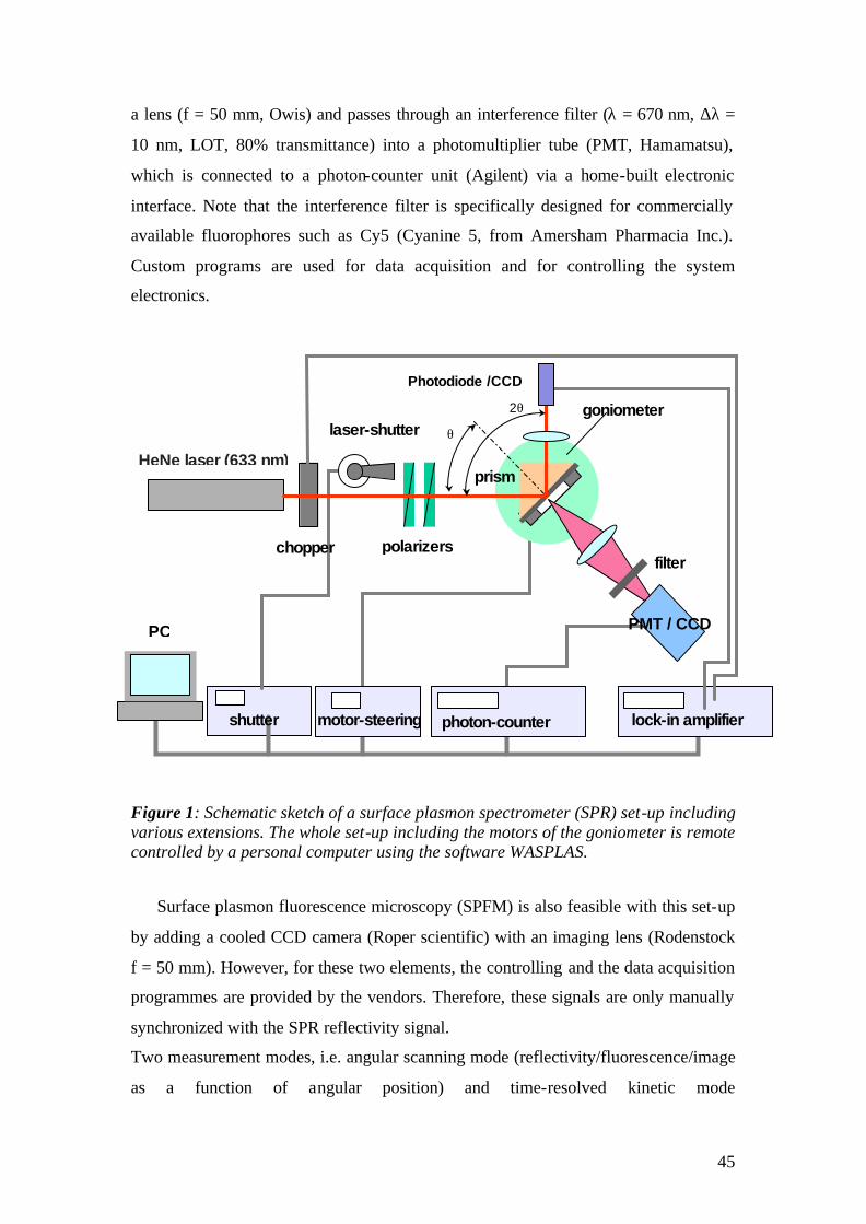
45
a lens (f = 50 mm, Owis) and passes through an interference filter (λ = 670 nm, ∆λ =
10 nm, LOT, 80% transmittance) into a photomultiplier tube (PMT, Hamamatsu),
which is connected to a photon-counter unit (Agilent) via a home-built electronic
interface. Note that the interference filter is specifically designed for commercially
available fluorophores such as Cy5 (Cyanine 5, from Amersham Pharmacia Inc.).
Custom programs are used for data acquisition and for controlling the system
electronics.
Figure 1: Schematic sketch of a surface plasmon spectrometer (SPR) set-up including various extensions. The whole set-up including the motors of the goniometer is remote controlled by a personal computer using the software WASPLAS.
Surface plasmon fluorescence microscopy (SPFM) is also feasible with this set-up
by adding a cooled CCD camera (Roper scientific) with an imaging lens (Rodenstock
f = 50 mm). However, for these two elements, the controlling and the data acquisition
programmes are provided by the vendors. Therefore, these signals are only manually
synchronized with the SPR reflectivity signal.
Two measurement modes, i.e. angular scanning mode (reflectivity/fluorescence/image
as a function of angular position) and time-resolved kinetic mode
HeNe laser (633 nm)
polarizers
Photodiode /CCD
filter
2θ goniometer
lock-in amplifier
PC
chopper
laser-shutter
PMT / CCD
shutter controller
prism
θ
photon-counter motor-steering
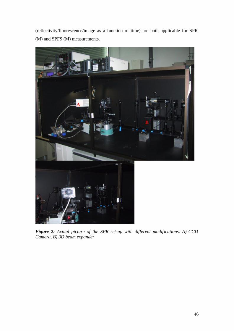
46
(reflectivity/fluorescence/image as a function of time) are both applicable for SPR
(M) and SPFS (M) measurements.
Figure 2: Actual picture of the SPR set-up with different modifications: A) CCD Camera, B) 3D beam expander
A
B
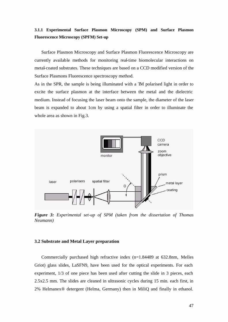
47
3.1.1 Experimental Surface Plasmon Microscopy (SPM) and Surface Plasmon
Fluorescence Microscopy (SPFM) Set-up
Surface Plasmon Microscopy and Surface Plasmon Fluorescence Microscopy are
currently available methods for monitoring real-time biomolecular interactions on
metal-coated substrates. These techniques are based on a CCD modified version of the
Surface Plasmons Fluorescence spectroscopy method.
As in the SPR, the sample is being illuminated with a TM polarised light in order to
excite the surface plasmon at the interface between the metal and the dielectric
medium. Instead of focusing the laser beam onto the sample, the diameter of the laser
beam is expanded to about 1cm by using a spatial filter in order to illuminate the
whole area as shown in Fig.3.
Figure 3: Experimental set-up of SPM (taken from the dissertation of Thomas Neumann)
3.2 Substrate and Metal Layer preparation
Commercially purchased high refractive index (n=1.84489 at 632.8nm, Melles
Griot) glass slides, LaSFN9, have been used for the optical experiments. For each
experiment, 1/3 of one piece has been used after cutting the slide in 3 pieces, each
2.5x2.5 mm. The slides are cleaned in ultrasonic cycles during 15 min. each first, in
2% Helmanex® detergent (Helma, Germany) then in MiliQ and finally in ethanol.

48
Before the slides are loaded into a thermal evaporation machine (Edwards, FL400
with ~2x10⁻⁶mbar UHV), they are dried under a stream of nitrogen and then placed
directly into the evaporation apparatus.
For standard SPR measurements, 53.5nm gold (99.99%, Balzers, Germany) was
deposited onto LaSFN9 glass substrates but since the experiments were carried out by
using a flow cell under saline buffer condition, additional ~ 1.5nm chromium layer
was evaporated first in order to increase the adhesion of the gold on the glass
substrate.
3.2.1 Self Assambled Monolayers (SAM) on gold
Self-assembled monolayers are known as molecular assemblies that are formed
spontaneously by immersion of a substrate into a solution of an active surfactant in an
organic solvent [Ulman, 1991]. From the thermodynamic point of view, several process
are known to promote the self assembly process on the surface: for example one
driving force could be physisorption. This process is not accompanied by a chemical
reaction but relies, e.g., on electrostatic interactions between adsorbed molecules. A
typical example is the alternating adsorption of polyelectrolyte layers of opposite
charge. SAMs are often further stabilized by interactions between neighboring
molecules in the film. Van der Walls interactions could be another example of
physisorption. Another driving force is chemisorption, which is based on the high
chemical affinity between the head group of the surfactant and the surface. These
interactions are strongly attractive and lead to the formation of a thermodynamically
favored covalent bond. As a result, molecules try to occupy every available binding
site on the surface as shown in Fig4-c.
During the present work, a binary mixture of alkene-thiols, except in studies in
chp.4.3.2, was routinely used to functionalize a gold surface. One of the molecules is
terminated with a biotin group for the subsequent streptavidin binding to the surface
architecture, while the other one which has a shorter chain length and is terminated
with a hydroxyl group that acts as a spacer to dilute the biotinylated species in control
of surface density. The chemical structures are shown in fig.4-a and b. The ratio of
spacer thiol to biotinylated thiol has been set at 9:1 in order to create optimized space
for the binding sites [Knoll, 2000]. The SAM was prepared ex-situ by immersion of a

49
gold slide in a 0.1 mM solution of thiols in EtOH overnight. After rinsing with EtOH,
the slide was dried in a nitrogen stream and mounted into the flow cell.
The typical picture for the chemisorption of thiols on gold is that the thiol loses its
hydrogen atom and becomes a thiolate covalently bound to the gold surface.
Two models for the reaction mechanism which only differ in the oxidant involved in
the reaction, which is either protons or oxygen are suggested in the literature [Ulman,
1991]
2H)I(AuSR2)0(Au2SHR2 +−−→+−
OH)I(AuSR2O21
)0(Au2SHR2 22 +−−→++−
(a). OH
HS (b) (c)
OHOH OHOHOH OHOH OHOHOHOH
OH
OH
OH
OH
OH
OHOH OHOHOH OHOH OHOH
anchor groupalkyl chainbiotin
Figure 4: Chemical structure of a) 1-mercapto-undecanole and b) 11-mercapto-(8-biotinamido-4, 7, dioxaoctyl-)-undecanoylamide, (c) Schematic of the self-assembly process. The anchor group, in this case S-H, has a strong chemical affinity to the gold surface. A covalent Au-S-bond is spontaneously formed by the mere exposure of the thiol solution to the gold surface. In the course of the reaction, all available binding sites on the gold surface are occupied by thiol molecules. The alkyl-chains adopt a parallel orientation with a uniform tilt angle of 30° relative to the surface normal. Such a highly ordered surface architecture meets perfectly the steric requirements for streptavidin binding (right cartoon).
O
Biotin moeity
HS O
N H
O O N
H
O S
N N H H
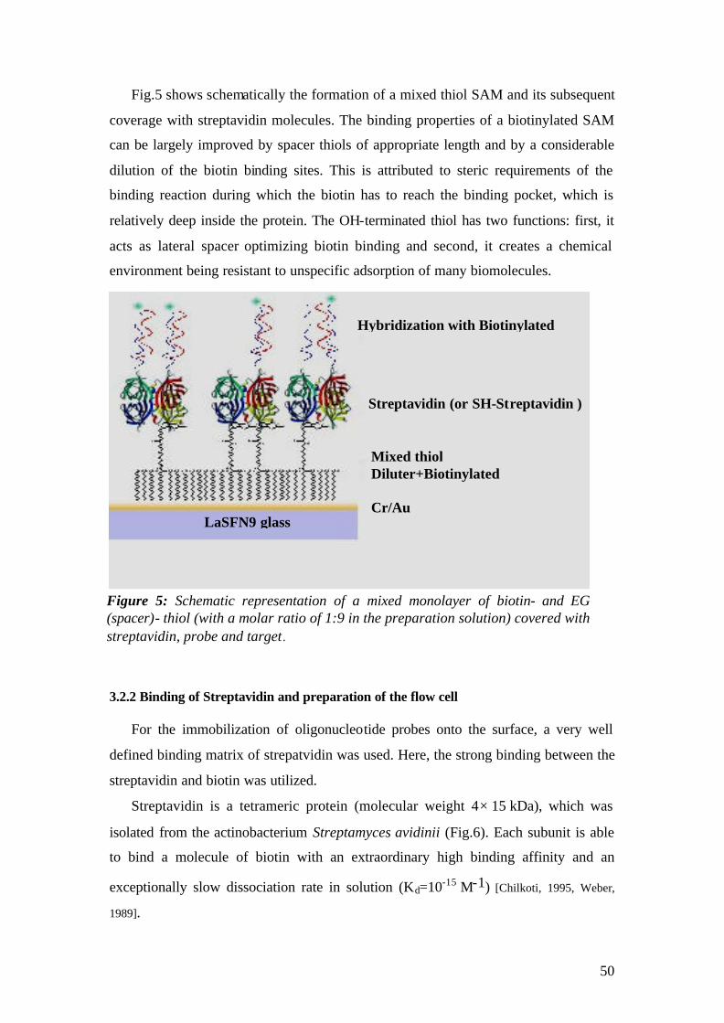
50
Fig.5 shows schematically the formation of a mixed thiol SAM and its subsequent
coverage with streptavidin molecules. The binding properties of a biotinylated SAM
can be largely improved by spacer thiols of appropriate length and by a considerable
dilution of the biotin binding sites. This is attributed to steric requirements of the
binding reaction during which the biotin has to reach the binding pocket, which is
relatively deep inside the protein. The OH-terminated thiol has two functions: first, it
acts as lateral spacer optimizing biotin binding and second, it creates a chemical
environment being resistant to unspecific adsorption of many biomolecules.
3.2.2 Binding of Streptavidin and preparation of the flow cell
For the immobilization of oligonucleotide probes onto the surface, a very well
defined binding matrix of strepatvidin was used. Here, the strong binding between the
streptavidin and biotin was utilized.
Streptavidin is a tetrameric protein (molecular weight 4 × 15 kDa), which was
isolated from the actinobacterium Streptamyces avidinii (Fig.6). Each subunit is able
to bind a molecule of biotin with an extraordinary high binding affinity and an
exceptionally slow dissociation rate in solution (Kd=10-15 M-1) [Chilkoti, 1995, Weber,
1989].
Mixed thiol Diluter+Biotinylated thiol
Streptavidin (or SH-Streptavidin )
Hybridization with Biotinylated
Cr/Au LaSFN9 glass
Figure 5: Schematic representation of a mixed monolayer of biotin- and EG (spacer)- thiol (with a molar ratio of 1:9 in the preparation solution) covered with streptavidin, probe and target .
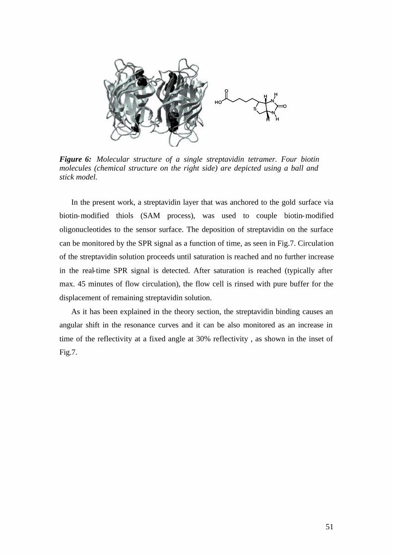
51
SOH
O
N
NH H
H
O
H
SOH
O
N
NH H
H
O
H
Figure 6: Molecular structure of a single streptavidin tetramer. Four biotin molecules (chemical structure on the right side) are depicted using a ball and stick model.
In the present work, a streptavidin layer that was anchored to the gold surface via
biotin-modified thiols (SAM process), was used to couple biotin-modified
oligonucleotides to the sensor surface. The deposition of streptavidin on the surface
can be monitored by the SPR signal as a function of time, as seen in Fig.7. Circulation
of the streptavidin solution proceeds until saturation is reached and no further increase
in the real-time SPR signal is detected. After saturation is reached (typically after
max. 45 minutes of flow circulation), the flow cell is rinsed with pure buffer for the
displacement of remaining streptavidin solution.
As it has been explained in the theory section, the streptavidin binding causes an
angular shift in the resonance curves and it can be also monitored as an increase in
time of the reflectivity at a fixed angle at 30% reflectivity , as shown in the inset of
Fig.7.
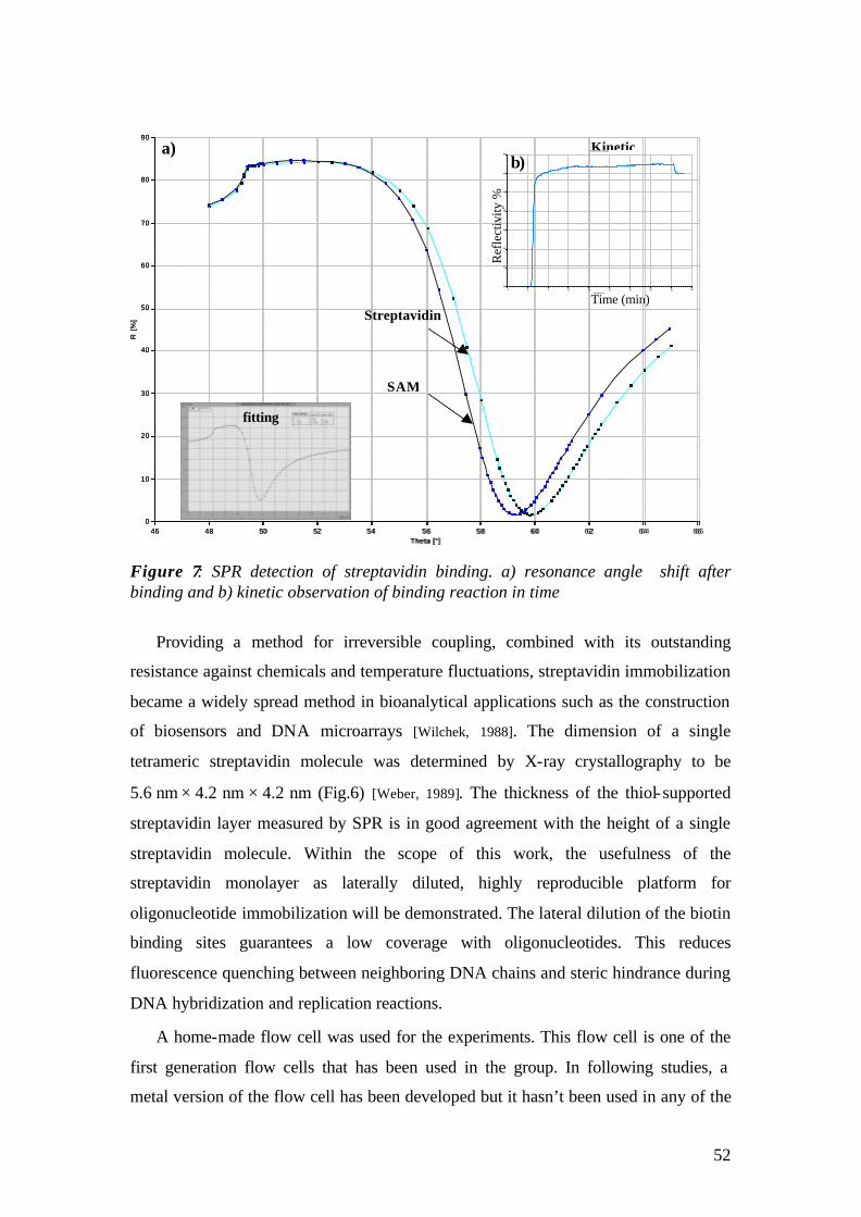
52
Figure 7: SPR detection of streptavidin binding. a) resonance angle shift after binding and b) kinetic observation of binding reaction in time
Providing a method for irreversible coupling, combined with its outstanding
resistance against chemicals and temperature fluctuations, streptavidin immobilization
became a widely spread method in bioanalytical applications such as the construction
of biosensors and DNA microarrays [Wilchek, 1988]. The dimension of a single
tetrameric streptavidin molecule was determined by X-ray crystallography to be
5.6 nm × 4.2 nm × 4.2 nm (Fig.6) [Weber, 1989]. The thickness of the thiol-supported
streptavidin layer measured by SPR is in good agreement with the height of a single
streptavidin molecule. Within the scope of this work, the usefulness of the
streptavidin monolayer as laterally diluted, highly reproducible platform for
oligonucleotide immobilization will be demonstrated. The lateral dilution of the biotin
binding sites guarantees a low coverage with oligonucleotides. This reduces
fluorescence quenching between neighboring DNA chains and steric hindrance during
DNA hybridization and replication reactions.
A home-made flow cell was used for the experiments. This flow cell is one of the
first generation flow cells that has been used in the group. In following studies, a
metal version of the flow cell has been developed but it hasn’t been used in any of the
Ref
lect
ivity
%
Time (min)
46 48 50 52 54 56 58 60 62 64 66Theta [°]
0
10
20
30
40
50
60
70
80
90R
[%
]Scan-Messung
46 48 50 52 54 56 58 60 62 64 66Theta [°]
0
10
20
30
40
50
60
70
80
90R
[%
]Scan-Messung
SAM
fitting
Streptavidin
- 5 0 5 10 15 20 25 30 35 40Zeit [min]
30
32
34
36
38
40
42
44
R [
%]
Kinetik-MessungKinetic a) b)

53
studies in this thesis due to the corrosive effect of NaOH used for regeneration
purposes.
Side and top views of the flow cell are shown in Fig.8. The cell is constructed
from a quartz plate (Herasil, Schott) with an inlet and an outlet (diameter=1 mm) at
the indicated positions. The circular inner part of the cell has a radius of 3 mm and a
height of 2 mm confining the volume to ~60 µl. In order to be able to image the whole
array, the same design of the flow cell with a larger diameter (~2.5mm) was used. The
flow cell is sandwiched between a quartz plate (Herasil, Schott) and a glass wafer
which is evaporation-coated with a thin gold film as described above. The gold
covered surface points towards the cell. The contact areas between these components
are sealed by Viton O-rings. A high refractive index prism (LaSFN9; n=1.845) is
mounted on top of the glass waver. In order to improve the coupling between the
incident light and the SP modes, the glass waver and prism are connected via a thin
film of refractive index-matching oil (n=1.7). The use of matching oil with a
refractive index lower than that of the prism is justified by the high vapour pressure of
oils exhibiting higher refractive indices. A metal sample holder keeps the sample in
place on the goniometer during the measurement. All measurements were performed
employing a constant flow rate of 2.5 ml/ min unless otherwise specified.
gold surface
quartz glass
index fluid glass slide
flow cell O-ring
prism
θ
peristaltic pump
sample
flow cell
Figure 8: Construction of the measurement chamber (left) and top view of the flow cell including a schematic of the circulation loop (right).
The flow cell is connected to a peristaltic pump (NovoChem) and the sample
reservoir using Tygon® tubes with an inner diameter of 0.76 mm. Thus a closed
circulation loop is formed which is disconnected during the injection phase. The total
volume of the loop for a 1mm diameter flow cell is around 300-400 µl, while the
larger one is around 700-800µL. Therefore injection volumes between 1-1.5 ml for
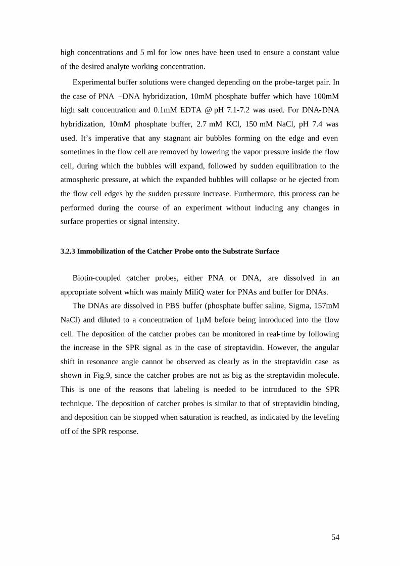
54
high concentrations and 5 ml for low ones have been used to ensure a constant value
of the desired analyte working concentration.
Experimental buffer solutions were changed depending on the probe-target pair. In
the case of PNA –DNA hybridization, 10mM phosphate buffer which have 100mM
high salt concentration and 0.1mM EDTA @ pH 7.1-7.2 was used. For DNA-DNA
hybridization, 10mM phosphate buffer, 2.7 mM KCl, 150 mM NaCl, pH 7.4 was
used. It’s imperative that any stagnant air bubbles forming on the edge and even
sometimes in the flow cell are removed by lowering the vapor pressure inside the flow
cell, during which the bubbles will expand, followed by sudden equilibration to the
atmospheric pressure, at which the expanded bubbles will collapse or be ejected from
the flow cell edges by the sudden pressure increase. Furthermore, this process can be
performed during the course of an experiment without inducing any changes in
surface properties or signal intensity.
3.2.3 Immobilization of the Catcher Probe onto the Substrate Surface
Biotin-coupled catcher probes, either PNA or DNA, are dissolved in an
appropriate solvent which was mainly MiliQ water for PNAs and buffer for DNAs.
The DNAs are dissolved in PBS buffer (phosphate buffer saline, Sigma, 157mM
NaCl) and diluted to a concentration of 1µM before being introduced into the flow
cell. The deposition of the catcher probes can be monitored in real- time by following
the increase in the SPR signal as in the case of streptavidin. However, the angular
shift in resonance angle cannot be observed as clearly as in the streptavidin case as
shown in Fig.9, since the catcher probes are not as big as the streptavidin molecule.
This is one of the reasons that labeling is needed to be introduced to the SPR
technique. The deposition of catcher probes is similar to that of streptavidin binding,
and deposition can be stopped when saturation is reached, as indicated by the leveling
off of the SPR response.
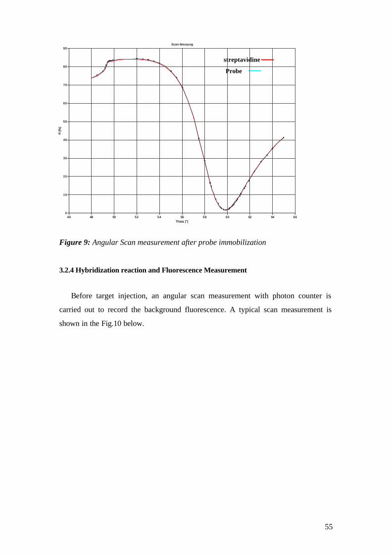
55
Figure 9: Angular Scan measurement after probe immobilization
3.2.4 Hybridization reaction and Fluorescence Measurement
Before target injection, an angular scan measurement with photon counter is
carried out to record the background fluorescence. A typical scan measurement is
shown in the Fig.10 below.
46 48 50 52 54 56 58 60 62 64 66Theta [°]
0
10
20
30
40
50
60
70
80
90
R [%
]
Scan-Messung
Probe
streptavidine
46 48 50 52 54 56 58 60 62 64 66Theta [°]
0
10
20
30
40
50
60
70
80
90
R [%
]
Scan-Messung

56
46 48 50 52 54 56 58 60 62 64 66Theta [°]
0
10
20
30
40
50
60
70
80
90
R [
%]
0
5.0E+4
1.0E+5
1.5E+5
2.0E+5
2.5E+5
3.0E+5
3.5E+5
Cou
nts
Scan-Messung
Figure 10: A typical SPR scan curve with the fluorescence (SPFS)
The fluorescence process was measured by increasing the angle of incidence
θincidence from 48 to 65° stepwise with ?θincidence= 0.1-0.5°. The angle of incidence
corresponding to the maximum fluorescence excitation (at θmax) can be easily
determined after the scan measurement and will be used as the fixed angle for kinetic
measurement for fluorescence. The experiments start by rinsing with buffer and then
recording a scan curve, which serves as the baseline of the experiment. In the single
kinetic experiment generally a 2ml volume of 100nM Cy5 dye labeled 11mer DNA
target solution was used. The first 500µl of the target solution was introduced into the
liquid handling system to replace the buffer solution from the flow cell and the
remaining 1.5ml were allowed to circulate within a closed loop during the experiment.
The measurement proceeds with a constant collection of the fluorescence intensity
data points with the help of a script, through which the shutter controller’s parameters
could be defined by the user. Usually the shutter was kept 3sec open in every data
point recorded in 5 min, to avoid bleaching of the chromophores.
Angle of incidence θ (degree)
Fluorescence intensity (cps) R
efle
ctiv
ity %
θmax
background
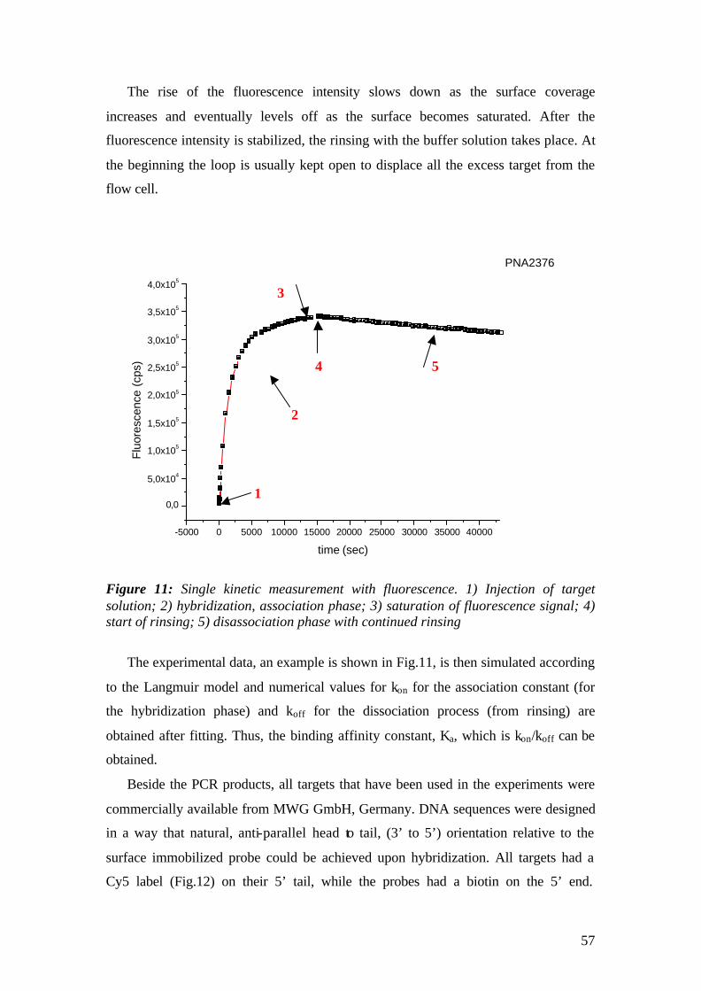
57
The rise of the fluorescence intensity slows down as the surface coverage
increases and eventually levels off as the surface becomes saturated. After the
fluorescence intensity is stabilized, the rinsing with the buffer solution takes place. At
the beginning the loop is usually kept open to displace all the excess target from the
flow cell.
-5000 0 5000 10000 15000 20000 25000 30000 35000 40000
0,0
5,0x10⁴
1,0x10⁵
1,5x10⁵
2,0x10⁵
2,5x10⁵
3,0x10⁵
3,5x10⁵
4,0x10⁵
Flu
ores
cenc
e (c
ps)
time (sec)
PNA2376
Figure 11: Single kinetic measurement with fluorescence. 1) Injection of target solution; 2) hybridization, association phase; 3) saturation of fluorescence signal; 4) start of rinsing; 5) disassociation phase with continued rinsing
The experimental data, an example is shown in Fig.11, is then simulated according
to the Langmuir model and numerical values for kon for the association constant (for
the hybridization phase) and koff for the dissociation process (from rinsing) are
obtained after fitting. Thus, the binding affinity constant, Ka, which is kon/koff can be
obtained.
Beside the PCR products, all targets that have been used in the experiments were
commercially available from MWG GmbH, Germany. DNA sequences were designed
in a way that natural, anti-parallel head to tail, (3’ to 5’) orientation relative to the
surface immobilized probe could be achieved upon hybridization. All targets had a
Cy5 label (Fig.12) on their 5’ tail, while the probes had a biotin on the 5’ end.
4
1
2
3
5

58
Depending on the purpose of the experiment, the target was designed to have either
full complementary base sequence to the probe (MM0, MisMatch0), a single base-pair
mismatched duplex (MM1) or a double base-pair mismatch duplex (MM2)
Figure 12: Chemical structure of Cy5 chromophore, which has its maximum absorbance at λ=649nm and emission at λ=670nm.
Due to the fact that all fluorescence measurements require highly sensitive signal
collection, some experimental considerations have to be kept in mind during the
experiment. Since a very small amount of stray light affects the fluorescence
background, the experimental set up is built in a black-box and the corners were
sealed with a black tape. Another consideration is the loss of the fluorescence signal
via quenching and bleaching. Self-bleaching occurs if the overall density of the
chromophores is too high. That process results in either re-absorbance or dissipation
of the fluorescence emission by neighbouring chromophores. This can be avoided
either by keeping the target concentration low or by reducing the density of binding
sites to ensure the separation between targets in solution and surface bound
chromophores. Photo-bleaching occurs when fluorescence emission is diminished due
to prolonged exposure to high energy excitations when the chromophore is chemically
of physically degraded. Photo-bleaching is a big problem especially in the
fluorescence microscopy experiments since the acqusition time is at least 20-25 sec.,
depending on the sensitivity of the CCD. Therefore either in the spectroscopy or in the
microscopy experiment, the laser light is blocked with the help of a shutter. Since the
titration experiments are longer than single kinetic experiments, the shutter control
becomes more crucial. That is why the closing time between two data points in that

59
kind of experiments is longer than that in a single kinetic experiment. Such strong
caution is needed not only because of the longer duration of the experiment, but also
in order to avoid self-bleaching of the chromophores due to the increase of the
surface-bound chromophore concentration in time.
A titration experiment is another method based on the Langmuir isotherm and
used for defining the binding properties of the oligonucletides. In this case, the surface
is being “decorated” by the target molecule starting from lower concentrations. The
surface probe architecture is allowed to be saturated by stepwise increase of the target
concentration according to the Langmuir isotherm. This condition has been obtained
by injection of the target solution with a specific concentration and by allowing
uninterrupted hybridization until the fluorescence signal reaches saturation. After
saturation, the target solution is replaced by the washing buffer and an angular
fluorescence scan is recorded. After the motor position is again tuned to the 30%
reflectivity angle, the second higher concentration is injected and the steps described
above repeated. This procedure is repeated until the fluorescence response no longer
shows a significant increase with increasing target concentration. The range of the
concentrations to be performed highly depends on the specific binding affinity
between surface the probe and the target. A titration experiment takes quite a long
time. Especially the first concentrations take a long time since the target binding
process at extreme low concentration is limited by mass transportation. The
possibility of material loss due to unspecific adsorption anywhere in the flow cell
during the circulation needs to be taken account at those extreme low concentrations,
e.g., pM as it is seen in Fig.13-a.
After the experimental data set is obtained, the fluorescence saturation values are
plotted against corresponding target concentration and the resulting plot is fitted to a
Langmuir isotherm (fig.13-b) in order to obtain the dissociation constant, Kd, which is
the reciprocal of the overall affinity constant Ka.

60
Figure 13: a) A typical titration experiment with a concentration range from pM to nM and b) obtaining the binding constant from Langmuir Isotherm fitting.
0 2000 4000 6000 8000 10000
0
50000
100000
150000
200000
250000
Data: Data1_BModel: Langmuir_iso Chi 2 = 306063608.32419R^2 = 0.96195 Rmax 214440 ±0Kd 66.63721
Flu
ores
cenc
e @
Sat
urat
ion
(cps
)
Concentration (pM)
PNA2367b)
0 1x10⁵ 2x10⁵ 3x10⁵ 4x10⁵ 5x10⁵ 6x10⁵ 7x10⁵
0
50000
100000
150000
200000
250000
Flu
ores
cenc
e (c
ps)
time (sec)
PNA2367
0.1pM 1pM 10pM
25pM
75pM
200pM
1nM
10nM
a)
0 50000 100000 150000 200000 250000
2000
4000
6000
8000
10000
Flu
ores
cenc
e (c
ps)
time (sec)
PNA2367
0.1 1
10
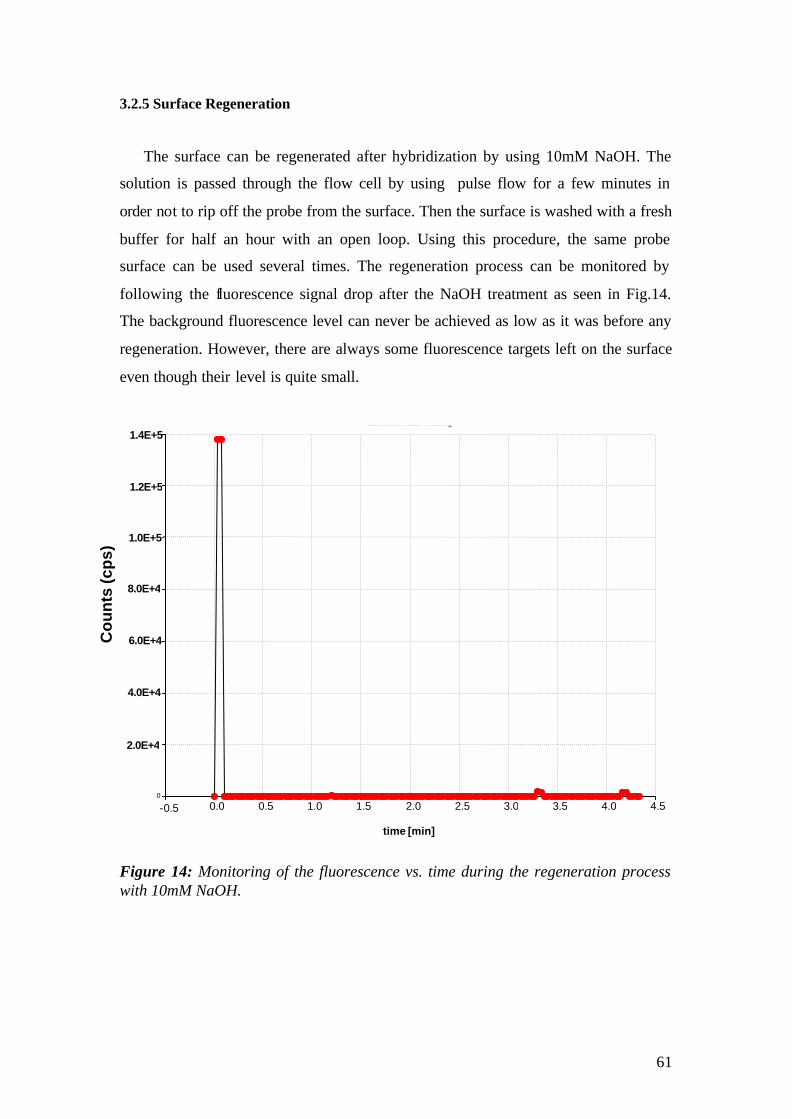
61
3.2.5 Surface Regeneration
The surface can be regenerated after hybridization by using 10mM NaOH. The
solution is passed through the flow cell by using pulse flow for a few minutes in
order not to rip off the probe from the surface. Then the surface is washed with a fresh
buffer for half an hour with an open loop. Using this procedure, the same probe
surface can be used several times. The regeneration process can be monitored by
following the fluorescence signal drop after the NaOH treatment as seen in Fig.14.
The background fluorescence level can never be achieved as low as it was before any
regeneration. However, there are always some fluorescence targets left on the surface
even though their level is quite small.
Figure 14: Monitoring of the fluorescence vs. time during the regeneration process with 10mM NaOH.
-0.5 0.0 0.5 1.0 1.5 2.0 2.5 3.0 3.5 4.0 4.5
time [min]
0
2.0E+4
4.0E+4
6.0E+4
8.0E+4
1.0E+5
1.2E+5
1.4E+5
Co
un
ts (c
ps)
Counter-Schreiber-Messung

62
3.3 Surface-Plasmon Fluorescence Miscroscopy – A Novel Platform for Array
Technology
3.3.1 Microarray preparation
Sample preparation steps involved basic glass slide cleaning, gold/chromium
evaporation, thiol/biothiol surface functionilization and then streptavidin and
biotinylated probe immobilization except for the SH-Streptavidin matrix. In later case,
instead of the thiol/biothiol step, thiolated streptavidin (SH-terminated Streptavidin,
Boehringer, Ingelheim, Germany) was used directly to the Au surface. The number of
the steps can be reduced using this approach but the fluorescent labeled target would
be brought closer to the metal surface and that will cause enhanced quenching by the
metal.
3.3.1.1 Array Fabrication
Cr/Au coated LaSFN9 glass slides were immersed into a OH-thiol/biotin-thiol
solution overnight, then washed with EtOH and incubated with 1µM Streptavidin for
more than an hour. Excess of streptavidin was washed away by MilliQ water and then
the samples were used immediately for spotting. A 1µM probe concentration has been
used for all arrays.
In the case of SH-Streptavidin, the freshly evaporated slide was incubated directly
in a 1µM SH-Streptavidin solution. It should be noted that, unless it’s not mentioned,
all the samples that were used in the experiments were prepared using the thiol
mixture/streptavidin/probe layer sequence.
The arrays have been prepared by using either an ink-jet piezo nanoplotter (cf.
Fig.4 in section 2.6.1), or a Pin- tool spotter (cf. Fig.5 in section 2.6.1) at room
temperature and 70% relative humidity conditions.
All arrays have been prepared by using PNA probes of different lengths and
mismatch carrying sequences in respect to the same target (MM0, MM1, MM2) given
in Table1 in section 4.3.

63
3.3.1.2 Array Characterization
SPM images were taken in air in order to determine the resonance angle from the
image contrast. In solution, however, the array usually was not detectable without
hybridization with the dye- labeled target due to low contrast.
3.3.2 Hybridization between PNA-probe and oligonucleotides-target
The sensor surface was functionalized by probe-PNAs of known sequences and
was exposed to an aqueous solution of the target-DNAs modified with Cy5
chromophore. A target can bind with a specific region to the probe sequence. The
length of the sequence will influence the specificity and sensitivity of the binding. The
rate constants and the affinity constants of the hybridization were measured for
different lengths of the sequence for both, MM0 and MM1 target-DNA, respectively
hybridizing to the probe-PNA strand in 10mM PB (10mM phosphate, 0.1 mM EDTA,
and 0.005 % Tween 20) buffer solution at room temperature.
The fluorescence increase was measured as a function of time after the target
molecules were injected until equilibrium was reached. After hybridization, a rinsing
process was performed by changing the fresh buffer solution continuously. Each
association and dissociation kinetics of hybridization was monitored by SPFM.
64
RESULTS
4. PNA-DNA Hybridization Observed in Real-Time
4.1 Surface Plasmon Field-Enhanced Fluorescence Spectroscopy (SPFS) studies
of PNA-DNA interaction on two-dimensional (planar) surfaces
In this chapter, we describe the PNA-DNA interaction quantified by the SPFS
technique. Different methods have been applied to describe the kinetic behaviour of
the duplex formation. Affinity constants of the each PNA were obtained from single
kinetic, titration and global analysis measurements and compared with their melting
temperature values determined in bulk solutions.
4.1.1 SPFS
Surface plasmon field–enhanced fluorescence spectroscopy (SPFS) uses the
enhanced electromagnetic field of a surface plasmon mode to excite surface confined
fluorophores. In our case, the evanescent field of a surface plasmon at the gold/water
interface is enhanced by a factor of 16 compared to incident field at the respective
resonance angle. It decays exponentially into the dielectric medium with a penetration
length of approximately 150 nm. Molecules in this evanescent layer alter the optical
properties of the interface and can be sensed by monitoring the changes in SPR
resonance minimum position. In the case of a molecule, carrying a fluorophore,
fluorescence emission will be excited by the plasmon field.
SPFS gives access to local refractive index change and the fluorophore
concentration simultaneously, it is thus a combinative technique, which gives more
precise information than the label- free technique SPR alone.
However, one has to take into account some limitations. In the SPFS measurement,
the fluorescence yield of a fluorophores near a metal exhibits highly pronounced
distance-dependent behaviour, as it was mentioned before in the theory section [Barnes,
1998]. If we look at the Fig.1, for separation distances, 20-30 nm, the fluorescence of
the fluorophore might be quenched or can be back-coupled as red-shifted re-radiation.
For the distances smaller that 20nm, the chromophore gives its energy back to the
metal layer as heat.

65
Figure 1: Decay channels for fluorescence emitted near a metallic surface A) non-radiative energy transfer, B) coupling of irradiated fluorescence light to SP modes, C) free emission of fluorescence.
Hence the effective fluorescence emission will be reduced. On the other hand, if
the distance between the metal layer and the fluorophore is increased further, the
fluorescence yield becomes weaker due to the fading evanescent field. This distance
dependent phenomena, however, might help to understand the conformation of the
surface bound molecules.
4.1.2 Experimental
4.1.2.1 Fluorescence monitoring
All the hybridization reactions were performed using Cy5 labeled targets which
were diluted by working buffer.
The fluorescence light emitted from dye- labeled probes was either monitored in
the scan or in the kinetic mode as described for the SPR spectra, with a PMT on the
backside of the flow cell switched on. If the use of fluorescent probes was limited to
surface reactions that were attributed to very low mass changes, the resonance angle
for SP excitation remained unchanged. As depicted in the SPFS scan spectrum before,
the fluorescence increased from the background value to a value determined by the
dye concentration. Thus, if the resonance curve of the SPs does not shift, a linear
relation between dye concentration and fluorescence intensity exists. The
quantification of the fluorescence signal in the kinetic mode is more complicated in
cases for which the resonance angle changes simultaneously with the surface
concentration of dye. Then, the intensity of the evanescent field of the SP changes for
a fixed angle of incidence and hence, the intensity of the excitation field. In this case,
Metal εm
Prism εp
Water εd
DyeD
ista
nce
d
(A) (B)
(C)
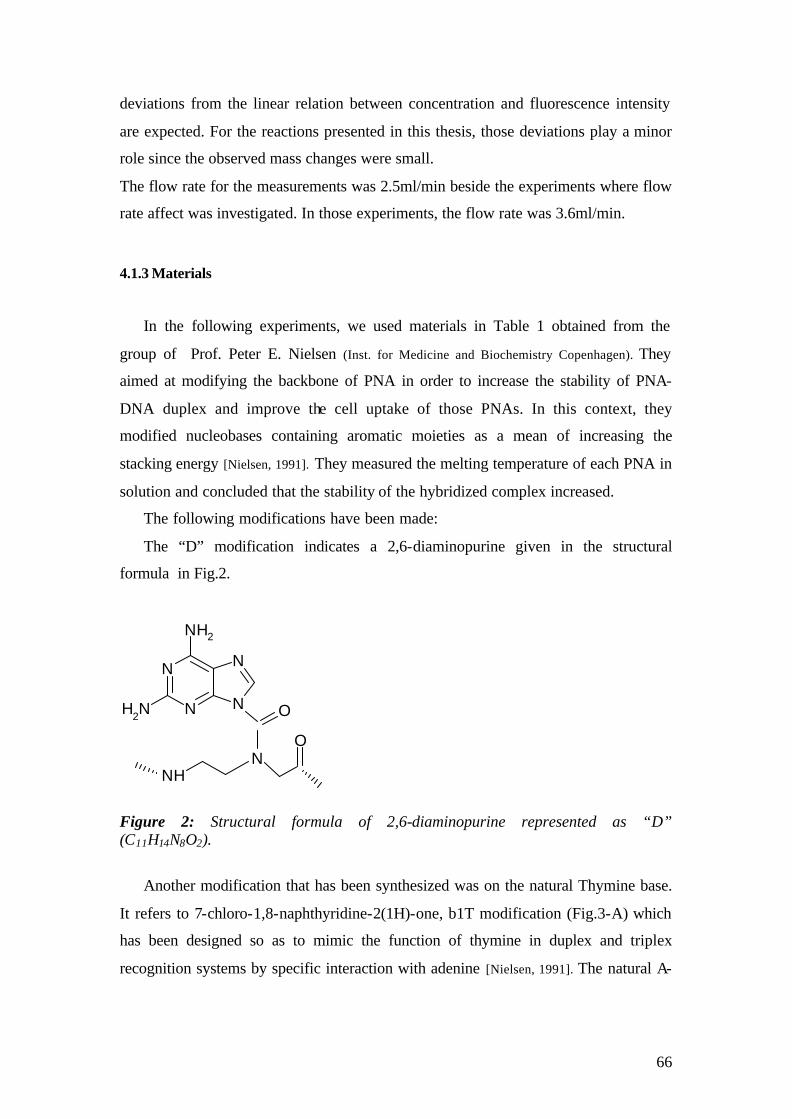
66
deviations from the linear relation between concentration and fluorescence intensity
are expected. For the reactions presented in this thesis, those deviations play a minor
role since the observed mass changes were small.
The flow rate for the measurements was 2.5ml/min beside the experiments where flow
rate affect was investigated. In those experiments, the flow rate was 3.6ml/min.
4.1.3 Materials
In the following experiments, we used materials in Table 1 obtained from the
group of Prof. Peter E. Nielsen (Inst. for Medicine and Biochemistry Copenhagen). They
aimed at modifying the backbone of PNA in order to increase the stability of PNA-
DNA duplex and improve the cell uptake of those PNAs. In this context, they
modified nucleobases containing aromatic moieties as a mean of increasing the
stacking energy [Nielsen, 1991]. They measured the melting temperature of each PNA in
solution and concluded that the stability of the hybridized complex increased.
The following modifications have been made:
The “D” modification indicates a 2,6-diaminopurine given in the structural
formula in Fig.2.
Figure 2: Structural formula of 2,6-diaminopurine represented as “D” (C11H14N8O2).
Another modification that has been synthesized was on the natural Thymine base.
It refers to 7-chloro-1,8-naphthyridine-2(1H)-one, b1T modification (Fig.3-A) which
has been designed so as to mimic the function of thymine in duplex and triplex
recognition systems by specific interaction with adenine [Nielsen, 1991]. The natural A-
N
NN
N
NH2
NH2 O
NNH
O

67
T base pair hybridization is shown in Fig.3-B. in both case, A-T and modified T-A
(Fig.4-A) have a specific recognition to adenine (Fig3-C).
Figure 3: A) Mimic of the neutral thymine nucleobase, 7-chloro-1,8-naphthyridine-2(1H)-one; The Watson-Crick base pair interaction B) between natural Adenin-Thymine, C) Adenine-Modified Thymine bases
A)
B) C)

68
Table 1: PNAs that were obtained from the Copenhagen group and the targets, which were commercially supplied from MWG, Germany.
Strands Sequence Tm
(°C)a ∆Tm (°C)b
∆Tm/mod (°C)b
PNA2361 5´-Biotin-(eg1)2-AGA GTC AGC TT-Lys-NH2
67.1 − −
PNA 2364 5´-Biotin-(eg1)2-DGA GTC AGC TT-Lys-NH2
68.3 1.2 1.2
PNA 2367 5´-Biotin-(eg1)2-DGD GTC AGC TT-Lys-NH2
73.4 6.3 3.2
PNA 2370 5´-Biotin-(eg1)2-DGD GTC DGC TT-Lys-NH2
77.1 10.0 3.3
PNA 2373 5´-Biotin-(eg1)2-AGA G(b1T)C AGC TT-Lys-NH2
69.2 2.1 2.1
PNA 2376 5´-Biotin-(eg1)2-AGA G(b1T)C AGC (b1T)T-Lys-NH2
70.2 3.1 1.1
PNA 2379 5´-Biotin-(eg1)2-AGA G(b1T)C AGC (b1T)(b1T)-Lys-NH2
71.2 4.1 1.4
Target Cy5-AAG CTG ACT CT-3`
SL15mer unspecific target
Cy5- CTAGTTCAGCAGCGA -3`
a. Duplex concentration is 5.0 µM in strands. b. The ‘+’ sign indicates an increase in the value with respect to the unmodified duplex. eg1: Ethylene Glycol spacer
One of the parameters that indicates the stability of the PNA-DNA duplex is the
melting temperature (Tm) of the PNAs. As it was found by Prof. Peter E. Nielsen’s
group [Nielsen et al., 2002] that the modification has shown an increase of the melting
temperatures corresponding to an increased of stability compared to the unmodified
PNA2361. The melting temperature and the temperature increase per modification are
in between 1.2 to 10 and 1.1 to 3.3 oC respectively.
Another parameter to describe the stability is the affinity constant (Ka). In the
following experiments Ka has been obtained using 3 independent measurements;
single kinetic measurement, titration measurement and global analysis measurements.
All experiments were performed in 10mM phosphate buffer containing 100mM NaCl

69
at pH 7.1-7.2. Single kinetic measurements were performed using 100nM target
unless otherwise mentioned.
The target used for the measurements has a Cy5 dye label, which is a negatively
charged molecule. On the other hand, Lysine which was inserted into the backbone in
order to increase the solubility of the PNA [Nielsen et al., 1991], is positively charged.
Therefore, first the effect of unspecific interaction between Lysine and the Cy5 dye
was investigated. A non-complementary 15mer target was injected and the
fluorescence signal monitored as it is shown in Fig.4. The intensity increases,
however, upon rinsing, the fluorescence dropped back to the background level. That
indicates that there is almost no unspecific binding.
Figure 4: Unspecific binding measurement between Lysine and dye.
4.1.4 Single kinetic measurements
Single kinetic measurements analyze the association and dissociation phases of
PNA-DNA hybridization. The association phase involves the hybridization process
with the target. After saturation is reached, rinsing is started. Thus the dissociation
phase is triggered.
0 2000 4000 6000 8000 10000 120000
2000
4000
6000
8000
10000
Flu
ores
cenc
e (c
ps)
time (sec)
PNA2370/target=100nM Cy5-labelled SL15mer MM0unspecific binding+Lysine-Cy5
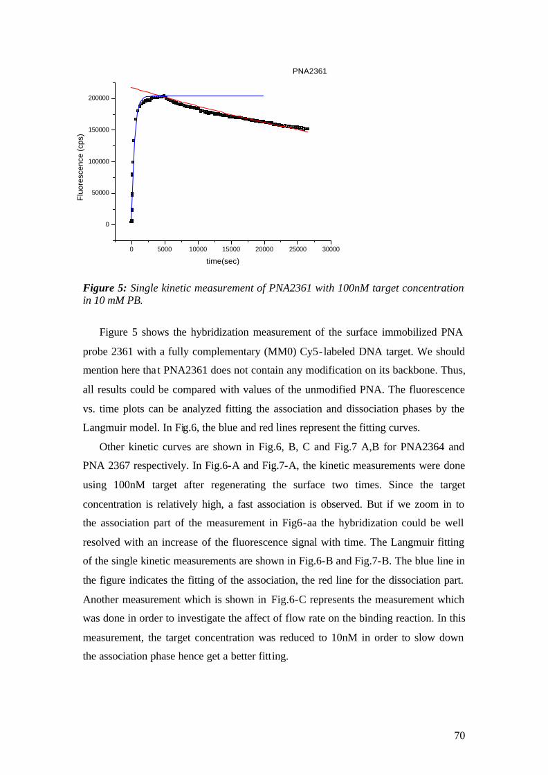
70
Figure 5: Single kinetic measurement of PNA2361 with 100nM target concentration in 10 mM PB.
Figure 5 shows the hybridization measurement of the surface immobilized PNA
probe 2361 with a fully complementary (MM0) Cy5- labeled DNA target. We should
mention here tha t PNA2361 does not contain any modification on its backbone. Thus,
all results could be compared with values of the unmodified PNA. The fluorescence
vs. time plots can be analyzed fitting the association and dissociation phases by the
Langmuir model. In Fig.6, the blue and red lines represent the fitting curves.
Other kinetic curves are shown in Fig.6, B, C and Fig.7 A,B for PNA2364 and
PNA 2367 respectively. In Fig.6-A and Fig.7-A, the kinetic measurements were done
using 100nM target after regenerating the surface two times. Since the target
concentration is relatively high, a fast association is observed. But if we zoom in to
the association part of the measurement in Fig6-aa the hybridization could be well
resolved with an increase of the fluorescence signal with time. The Langmuir fitting
of the single kinetic measurements are shown in Fig.6-B and Fig.7-B. The blue line in
the figure indicates the fitting of the association, the red line for the dissociation part.
Another measurement which is shown in Fig.6-C represents the measurement which
was done in order to investigate the affect of flow rate on the binding reaction. In this
measurement, the target concentration was reduced to 10nM in order to slow down
the association phase hence get a better fitting.
0 5000 10000 15000 20000 25000 30000
0
50000
100000
150000
200000
Flu
ores
cenc
e (c
ps)
time(sec)
PNA2361

71
Figure 6: A) Single kinetic measurement of PNA2364 and B) its Langmuir fit with the flow rate 2.5ml/min. C) same kinetic measurement with a faster flow rate, 3.6ml/min and using 10nM target concentration and zoomed-in plot of association (small graph)
0 5000 10000 15000 20000
0,0
5,0x10⁴
1,0x10⁵
1,5x10⁵
2,0x10⁵
Flu
ores
cenc
e (c
ps)
time(sec)
PNA2364/part of single kinetic
B)
C)
0 5000 10000 15000 20000
0
50000
100000
150000
200000
250000
PNA2364-10nM-3.6ml/min faster flow rate/Partial
time (sec)
Flu
ores
cenc
e (c
ps)
0 5000
0
90000
180000
A)
-10000 0 10000 20000 30000 40000 50000 60000 70000 80000
0
50000
100000
150000
200000
Flu
ores
cenc
e (c
ps)
time (sec)
PNA2364-100nM, after 2xregen
0 500 1000 1500 2000
0
50000
100000
150000
200000
Fluo
resc
ence
(cps
)time(sec)
PNA2364/part of single kineticaa)
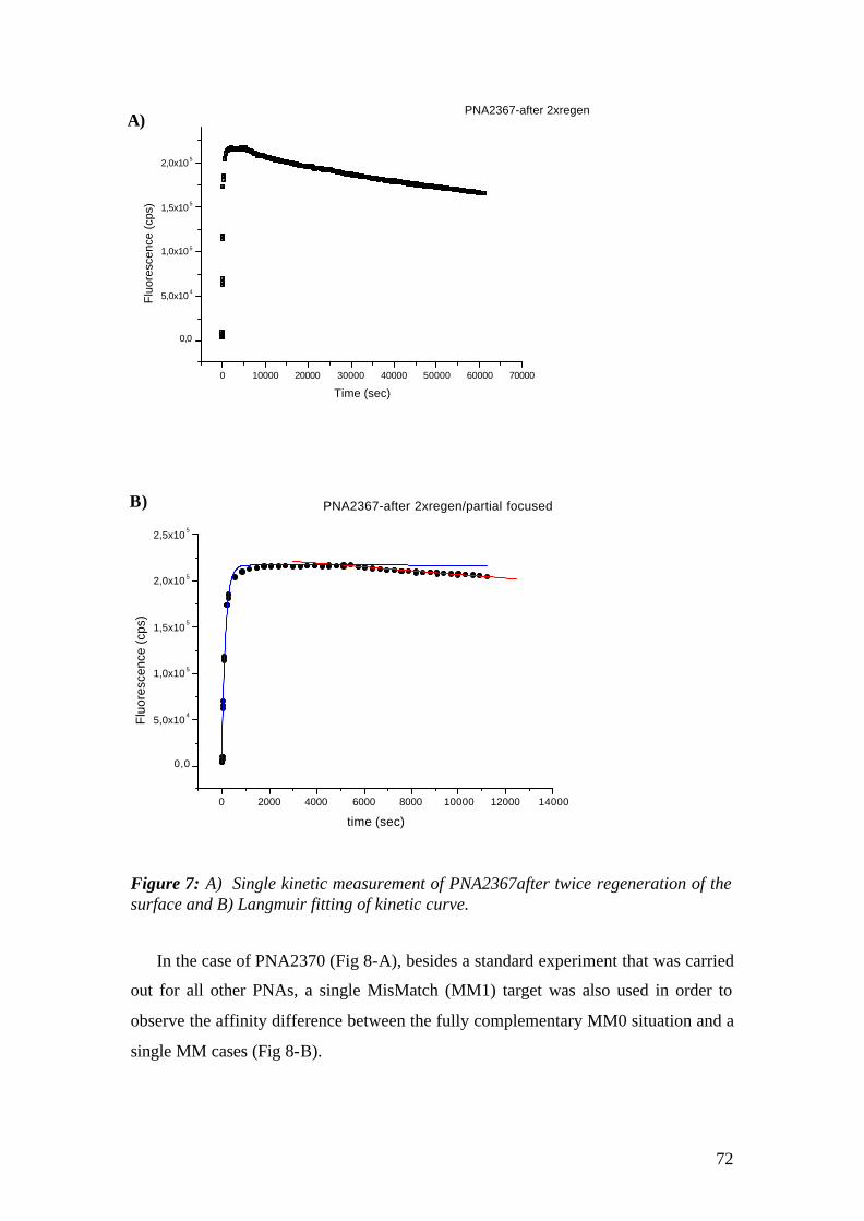
72
Figure 7: A) Single kinetic measurement of PNA2367after twice regeneration of the surface and B) Langmuir fitting of kinetic curve. In the case of PNA2370 (Fig 8-A), besides a standard experiment that was carried
out for all other PNAs, a single MisMatch (MM1) target was also used in order to
observe the affinity difference between the fully complementary MM0 situation and a
single MM cases (Fig 8-B).
0 2000 4000 6000 8000 10000 12000 14000
0,0
5,0x10⁴
1,0x10 5
1,5x10⁵
2,0x10 5
2,5x10⁵
Flu
ores
cenc
e (c
ps)
time (sec)
PNA2367-after 2xregen/partial focusedB)
0 10000 20000 30000 40000 50000 60000 70000
0,0
5,0x10⁴
1,0x10⁵
1,5x10⁵
2,0x10⁵
Flu
ores
cenc
e (c
ps)
Time (sec)
PNA2367-after 2xregenA)
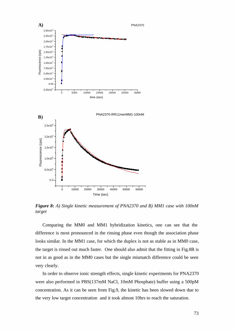
73
Figure 8: A) Single kinetic measurement of PNA2370 and B) MM1 case with 100nM target
Comparing the MM0 and MM1 hybridization kinetics, one can see that the
difference is most pronounced in the rinsing phase even though the association phase
looks similar. In the MM1 case, for which the duplex is not as stable as in MM0 case,
the target is rinsed out much faster. One should also admit that the fitting in Fig.8B is
not in as good as in the MM0 cases but the single mismatch difference could be seen
very clearly.
In order to observe ionic strength effects, single kinetic experiments for PNA2370
were also performed in PBS(137mM NaCl, 10mM Phosphate) buffer using a 500pM
concentration. As it can be seen from Fig.9, the kinetic has been slowed down due to
the very low target concentration and it took almost 10hrs to reach the saturation.
0 5000 10000 15000 20000 25000 30000-2,50x10
4
0,00
2,50x10 4
5,00x10⁴
7,50x10⁴
1,00x10⁵
1,25x10 5
1,50x10 5
1,75x10⁵
2,00x10⁵
2,25x10 5
2,50x10 5
Flu
ores
cenc
e (c
ps)
time (sec)
PNA2370A)
0 10000 20000 30000 40000 50000 60000
0,0
5,0x10⁴
1,0x10⁵
1,5x10⁵
2,0x10⁵
2,5x10⁵
Flu
ores
cenc
e (c
ps)
Time (sec)
PNA2370-RR11merMM1-100nMB)
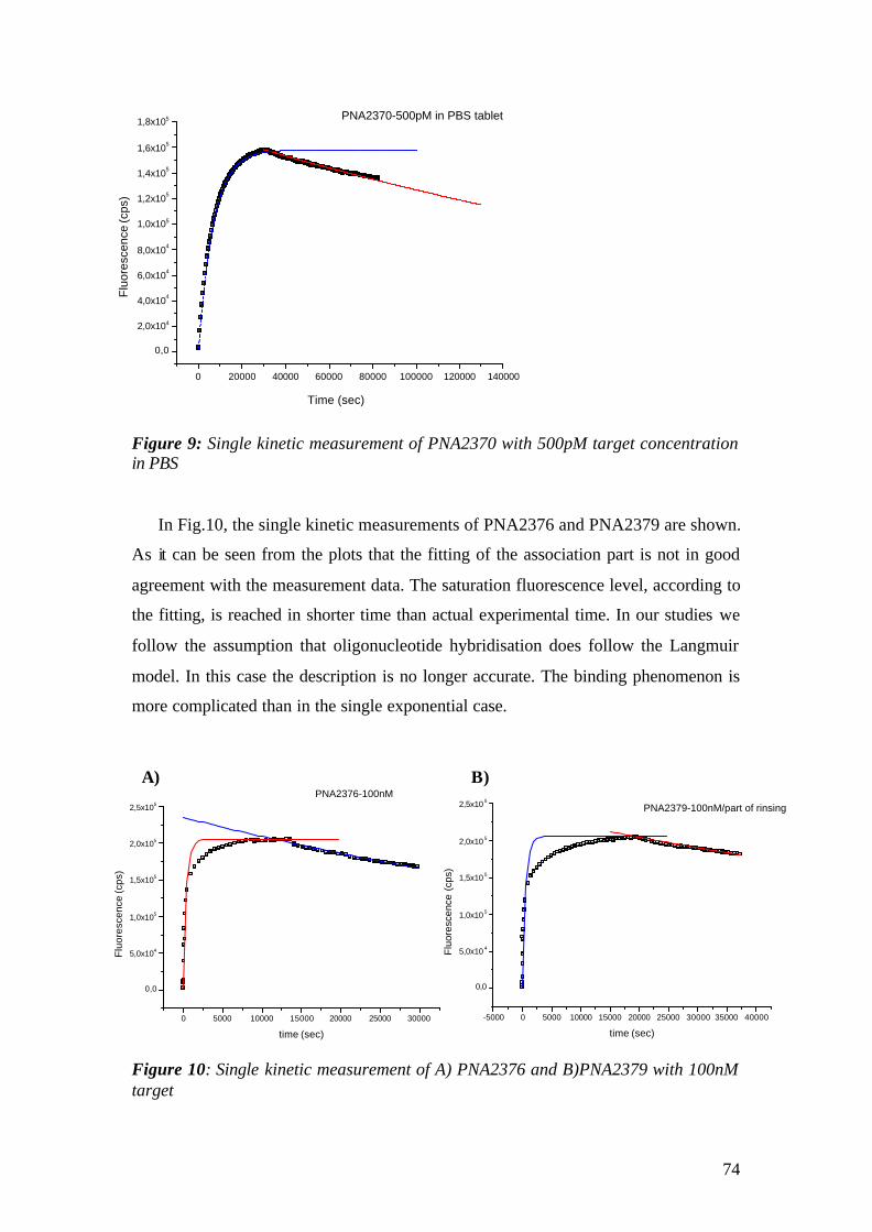
74
Figure 9: Single kinetic measurement of PNA2370 with 500pM target concentration in PBS In Fig.10, the single kinetic measurements of PNA2376 and PNA2379 are shown.
As it can be seen from the plots that the fitting of the association part is not in good
agreement with the measurement data. The saturation fluorescence level, according to
the fitting, is reached in shorter time than actual experimental time. In our studies we
follow the assumption that oligonucleotide hybridisation does follow the Langmuir
model. In this case the description is no longer accurate. The binding phenomenon is
more complicated than in the single exponential case.
Figure 10: Single kinetic measurement of A) PNA2376 and B)PNA2379 with 100nM target
0 20000 40000 60000 80000 100000 120000 140000
0,0
2,0x10⁴
4,0x10⁴
6,0x10⁴
8,0x10⁴
1,0x10⁵
1,2x10⁵
1,4x10⁵
1,6x10⁵
1,8x10⁵F
luor
esce
nce
(cps
)PNA2370-500pM in PBS tablet
Time (sec)
0 5000 10000 15000 20000 25000 30000
0,0
5,0x10⁴
1,0x10⁵
1,5x10⁵
2,0x10⁵
2,5x10⁵
Flu
ores
cenc
e (c
ps)
time (sec)
PNA2376-100nM
-5000 0 5000 10000 15000 20000 25000 30000 35000 40000
0,0
5,0x10 4
1,0x10 5
1,5x10 5
2,0x10 5
2,5x10 5
Flu
ores
cenc
e (c
ps)
time (sec)
PNA2379-100nM/part of rinsing
A) B)
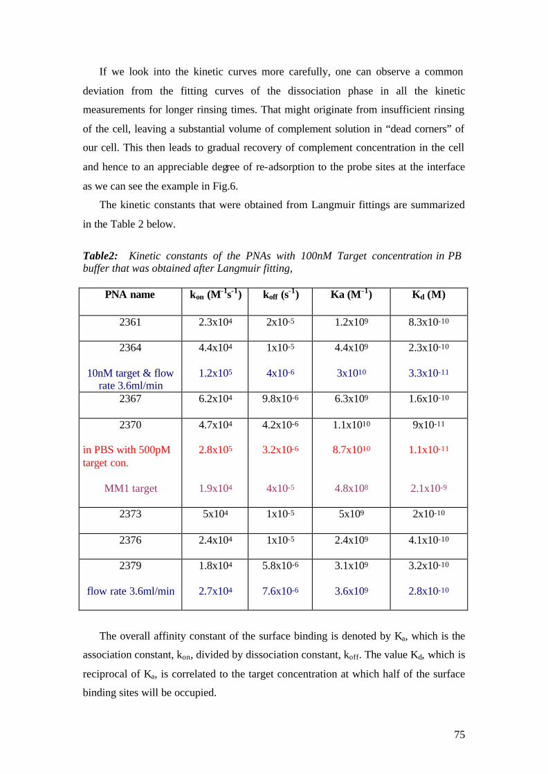
75
If we look into the kinetic curves more carefully, one can observe a common
deviation from the fitting curves of the dissociation phase in all the kinetic
measurements for longer rinsing times. That might originate from insufficient rinsing
of the cell, leaving a substantial volume of complement solution in “dead corners” of
our cell. This then leads to gradual recovery of complement concentration in the cell
and hence to an appreciable degree of re-adsorption to the probe sites at the interface
as we can see the example in Fig.6.
The kinetic constants that were obtained from Langmuir fittings are summarized
in the Table 2 below.
Table2: Kinetic constants of the PNAs with 100nM Target concentration in PB buffer that was obtained after Langmuir fitting,
PNA name kon (M-1s-1) koff (s-1) Ka (M-1) Kd (M)
2361 2.3x10⁴ 2x10⁻⁵ 1.2x10⁹
8.3x10⁻¹⁰
2364
10nM target & flow rate 3.6ml/min
4.4x10⁴
1.2x10⁵
1x10⁻⁵
4x10⁻⁶
4.4x10⁹
3x10¹⁰
2.3x10⁻¹⁰
3.3x10⁻¹¹
2367
6.2x10⁴
9.8x10⁻⁶
6.3x10⁹
1.6x10⁻¹⁰
2370
in PBS with 500pM target con.
MM1 target
4.7x10⁴
2.8x10⁵
1.9x10⁴
4.2x10⁻⁶
3.2x10⁻⁶
4x10⁻⁵
1.1x10¹⁰
8.7x10¹⁰
4.8x10⁸
9x10-11
1.1x10⁻¹¹
2.1x10⁻⁹
2373
5x10⁴ 1x10⁻⁵ 5x10⁹ 2x10⁻¹⁰
2376
2.4x10⁴ 1x10⁻⁵ 2.4x10⁹ 4.1x10⁻¹⁰
2379
flow rate 3.6ml/min
1.8x10⁴
2.7x10⁴
5.8x10⁻⁶
7.6x10⁻⁶
3.1x10⁹
3.6x10⁹
3.2x10⁻¹⁰
2.8x10⁻¹⁰
The overall affinity constant of the surface binding is denoted by Ka, which is the
association constant, kon, divided by dissociation constant, koff. The value Kd, which is
reciprocal of Ka, is correlated to the target concentration at which half of the surface
binding sites will be occupied.
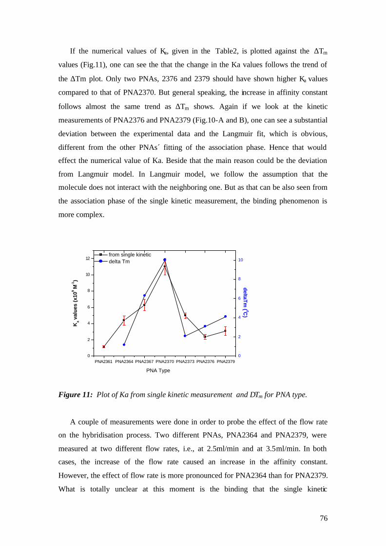
76
If the numerical values of Ka, given in the Table2, is plotted against the ∆Tm
values (Fig.11), one can see the that the change in the Ka values follows the trend of
the ∆Tm plot. Only two PNAs, 2376 and 2379 should have shown higher Ka values
compared to that of PNA2370. But general speaking, the increase in affinity constant
follows almost the same trend as ∆Tm shows. Again if we look at the kinetic
measurements of PNA2376 and PNA2379 (Fig.10-A and B), one can see a substantial
deviation between the experimental data and the Langmuir fit, which is obvious,
different from the other PNAs´ fitting of the association phase. Hence that would
effect the numerical value of Ka. Beside that the main reason could be the deviation
from Langmuir model. In Langmuir model, we follow the assumption that the
molecule does not interact with the neighboring one. But as that can be also seen from
the association phase of the single kinetic measurement, the binding phenomenon is
more complex.
PNA2361 PNA2364 PNA2367 PNA2370 PNA2373 PNA2376 PNA23790
2
4
6
8
10
12
PNA Type
Ka v
alue
s (x
109 M
-1)
from single kinetic delta Tm
0
2
4
6
8
10
deltaTm ( 0C
)
Figure 11: Plot of Ka from single kinetic measurement and ∆Tm for PNA type.
A couple of measurements were done in order to probe the effect of the flow rate
on the hybridisation process. Two different PNAs, PNA2364 and PNA2379, were
measured at two different flow rates, i.e., at 2.5ml/min and at 3.5ml/min. In both
cases, the increase of the flow rate caused an increase in the affinity constant.
However, the effect of flow rate is more pronounced for PNA2364 than for PNA2379.
What is totally unclear at this moment is the binding that the single kinetic

77
experiments with two different concentrations in the PNA 2364 result in a changed Ka
value in clear disagreement with the Langmuir picture. Some discrepancies in the
fitting of the association phase due to faster binding and not enough data points
collected (in order to avoid photobleaching) might also contribute to that result.
In the case of PNA2370, another measurement related to mismatch discrimination
was performed. As it can be seen from the Ka values, the difference between the
affinities of MM0 and MM1 is about 2 order of magnitude. The difference comes
from both, the association and the dissociation constants: in the case of MM1, the
target hybridisation with the probe is slower and the target dissociates faster upon
rinsing. That clearly indicates that mismatch discrimination by using PNA can be a
promising way for future applications.
4.1.5 Titration experiments
Titration experiments were performed to further elucidate the hybridization
behavior of the PNA probes. By this approach, we aimed to establishe a better
correlation of the values shown in Table 2. Titration experiments are also technically
significant because they offer a way to obtain Ka directly by quantifying the
correlation between the bulk target concentration and the surface cove rage. In a
titration experiment, the concentrations are chosen according to the Kd value of the
probe, obtained from single kinetic experiments. The starting concentration has to be
much lower than the Kd value with the final concentration being substantia lly higher
in order to fully saturate the probe surface. After reaching saturation, an angular scan
is performed to correlate the surface coverage with the obtained fluorescence
intensity. The maximum fluorescence values from the angular scan curve for each
concentrations are plotted against the concentration.
Fig.12-A, shows a titration experiment for PNA2361 along with the resulting plots
illustrating the conventional (Fig12-B) and the linearized (Fig12-C) relationship
between target concentration and corresponding saturation intensity. The range of the
target concentration that has been chosen for the titration experiment was defined
according to the Kd values obtained from the single kinetic measurements of each
PNA. As it was described before, the Kd value gives the target concentration at which
50% surface coverage is achieved. Since the Kd values of the PNAs are in the 10-10
range, starting target concentration in the pM range were chosen.
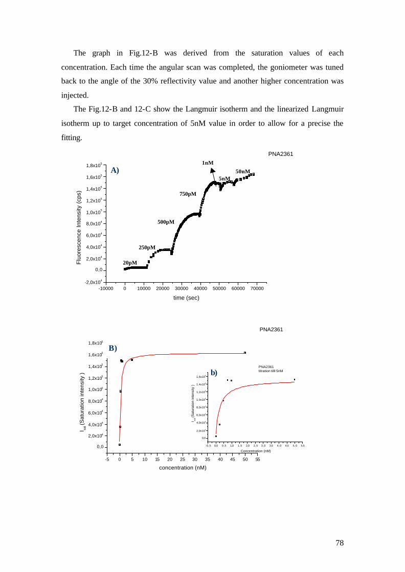
78
The graph in Fig.12-B was derived from the saturation values of each
concentration. Each time the angular scan was completed, the goniometer was tuned
back to the angle of the 30% reflectivity value and another higher concentration was
injected.
The Fig.12-B and 12-C show the Langmuir isotherm and the linearized Langmuir
isotherm up to target concentration of 5nM value in order to allow for a precise the
fitting.
-10000 0 10000 20000 30000 40000 50000 60000 70000-2,0x10⁴
0,0
2,0x10⁴
4,0x10⁴
6,0x10⁴
8,0x10⁴
1,0x10⁵
1,2x10⁵
1,4x10⁵
1,6x10⁵
1,8x10⁵
Flu
ores
cenc
e In
tens
ity (
cps)
time (sec)
PNA2361
20pM
250pM
500pM
750pM
1nM
5nM 50nM A)
-5 0 5 10 15 20 25 30 35 40 45 50 55
0,0
2,0x10⁴
4,0x10⁴
6,0x10⁴
8,0x10⁴
1,0x10⁵
1,2x10⁵
1,4x10⁵
1,6x10⁵
1,8x10⁵
I sat (
Sat
urat
ion
inte
nsity
)
concentration (nM)
PNA2361
-0,5 0,0 0,5 1,0 1,5 2,0 2,5 3,0 3,5 4,0 4,5 5,0 5,5
0,0
2,0x10⁴
4,0x10⁴
6,0x10⁴
8,0x10⁴
1,0x10⁵
1,2x10⁵
1,4x10⁵
1,6x10⁵
I sat (S
atur
atio
n in
tens
ity )
Concentration (nM)
PNA2361titration tilll 5nM
B)
b)

79
Figure 12: Titration curve of PNA2361 A) MM0 titration experiment B) conventional representation and C) linearized isotherm plots relating target concentrations with respective saturation intensity and b) and c) focused plots of B) and C) respectively.
As it can be seen from Fig12, a satisfying level of agreement is found between the
experimental data points and the fitting curve in the conventional plot 12-B. However,
discrepancies in the fitting can be seen more clearly if the curve is linearized.
The Langmuir isotherm can be also obtained from fluorescence scans taken after
each target concentration had reached saturation in the same titration measurement.
Since the fluorescence angular scan is following the surface coverage, the same
Langmuir picture can be seen.
Figure 13: Angular scan with fluorescence after saturation of each target concentration in the titration measurement.
4 4 4 6 4 8 5 0 5 2 5 4 5 6 5 8 6 0 6 2 6 4 6 6T h e t a [ ° ]
0
1 0
2 0
3 0
4 0
5 0
6 0
7 0
8 0
R [
%]
0
5 . 0 E + 4
1 . 0 E + 5
1 . 5 E + 5
2 . 0 E + 5
2 . 5 E + 5
3 . 0 E + 5
3 . 5 E + 5
Cou
nts
S c a n - M e s s u n g
a
b
c
d
e
f
g h
a) background b) 20pM c) 250pM d) 500pM g) 750pM e) 1nm f) 5nM h) 50nM
Angular scan (θ)
Counts (cps)
Ref
lect
ivit
y (%
)
Scan measurement
Imax
-5 0 5 10 15 20 25 30 35 40 45 50 55
0,0
5,0x10⁻⁵
1,0x10⁻⁴
1,5x10⁻⁴
2,0x10⁻⁴
2,5x10⁻⁴
3,0x10⁻⁴
3,5x10⁻⁴
Co/I fl (
nM/c
ps)
Concentration (nM)
-1 0 1 2 3 4 5 6 7
0,0
5,0x10⁻⁵
C)
c)
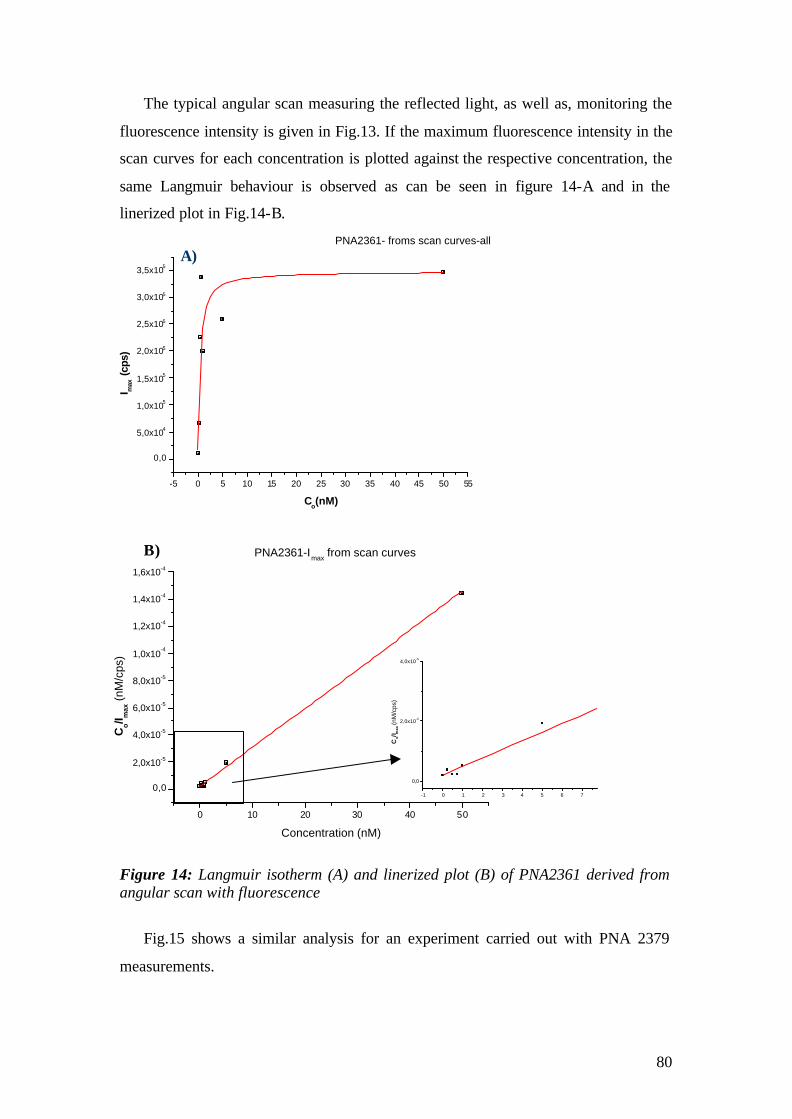
80
The typical angular scan measuring the reflected light, as well as, monitoring the
fluorescence intensity is given in Fig.13. If the maximum fluorescence intensity in the
scan curves for each concentration is plotted against the respective concentration, the
same Langmuir behaviour is observed as can be seen in figure 14-A and in the
linerized plot in Fig.14-B.
Figure 14: Langmuir isotherm (A) and linerized plot (B) of PNA2361 derived from angular scan with fluorescence
Fig.15 shows a similar analysis for an experiment carried out with PNA 2379
measurements.
-5 0 5 10 15 20 25 30 35 40 45 50 55
0,0
5,0x10⁴
1,0x10⁵
1,5x10⁵
2,0x10⁵
2,5x10⁵
3,0x10⁵
3,5x10⁵
I max
(cps
)
Co(nM)
PNA2361- froms scan curves-all
A)
0 10 20 30 40 50
0,0
2,0x10⁻⁵
4,0x10⁻⁵
6,0x10⁻⁵
8,0x10⁻⁵
1,0x10⁻⁴
1,2x10⁻⁴
1,4x10⁻⁴
1,6x10⁻⁴
Co/I m
ax (n
M/c
ps)
Concentration (nM)
PNA2361-Imax from scan curves
-1 0 1 2 3 4 5 6 7
0,0
2,0x10⁻⁵
4,0x10⁻⁵
Co/
I max
(nM
/cps
)
B)
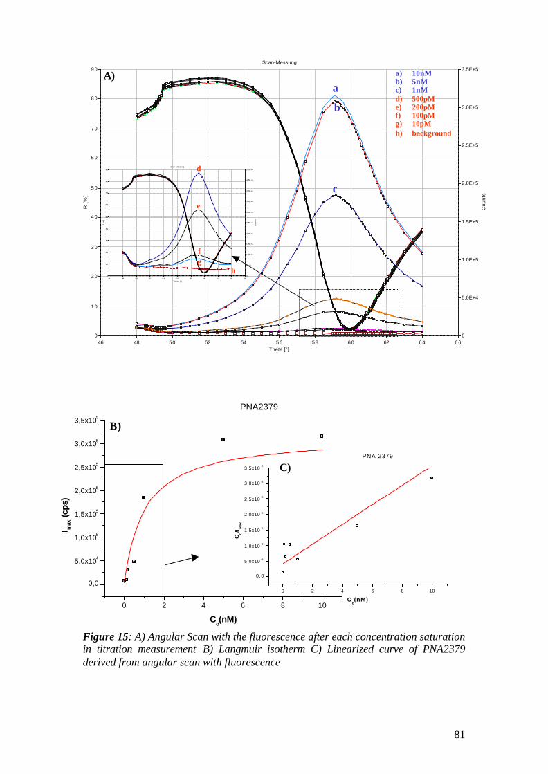
81
Figure 15: A) Angular Scan with the fluorescence after each concentration saturation in titration measurement B) Langmuir isotherm C) Linearized curve of PNA2379 derived from angular scan with fluorescence
0 2 4 6 8 10
0,0
5,0x10⁴
1,0x10⁵
1,5x10⁵
2,0x10⁵
2,5x10⁵
3,0x10⁵
3,5x10⁵
I max
(cp
s)
Co(nM)
PNA2379
0 2 4 6 8 10
0,0
5,0x10 -6
1,0x10 -5
1,5x10 -5
2,0x10 -5
2,5x10 -5
3,0x10 -5
3,5x10 -5
C0/I m
ax
Co(nM)
PNA 2379
B)
C)
46 48 50 52 54 56 58 60 62 64 66Theta [°]
0
10
20
30
40
50
60
70
80
90
R [
%]
0
5.0E+4
1.0E+5
1.5E+5
2.0E+5
2.5E+5
3.0E+5
3.5E+5
Cou
nts
Scan-Messung
a) 10nM b) 5nM c) 1nM d) 500pM e) 200pM f) 100pM g) 10pM h) background
a
b
c
46 48 5 0 52 5 4 5 6 58 60 6 2 64 66Theta [°]
0
1 0
2 0
3 0
4 0
5 0
6 0
7 0
8 0
9 0
R [
%]
0
5000
1.0E+4
1.5E+4
2.0E+4
2.5E+4
3.0E+4
3.5E+4
4.0E+4
4.5E+4
5.0E+4
Co
un
ts
Scan-Messung d
e
fg
h
A)

82
The fitting in Fig.15 is not in good agreement with the data. If we look at the scan
curve of the PNA2379, one can see that the increment in the Imax values of 10, 100
and 200pM samples are just above the background level. Because of those low
concentrations, the fitting shows some disagreement with the expected Langmuirian
behavior.
Equivalent titration curves for PNA2373 and the derived isotherms are given in
Fig.16A and B. Since the titration measurements are carried out using different
concentrations of the target, each step refers to the association phase of a single
kinetic measurement. Hence we can fit the association phase for each concentration
and obtain concentration dependent kon values. Since the disassociation is independent
of the concentration (according to the Langmuir model), koff values from a single
kinetic measurement were used in the calculation of the affinity constant. Different to
that approach, the koff values for PNA2370 were obtained from Langmuir fitting for
each rinsing step during the titration measurement. It can be seen from Fig.17 that the
koff values, indeed, do not change with concentration confirming the assumption made
above based on the Langmuir model predictions.
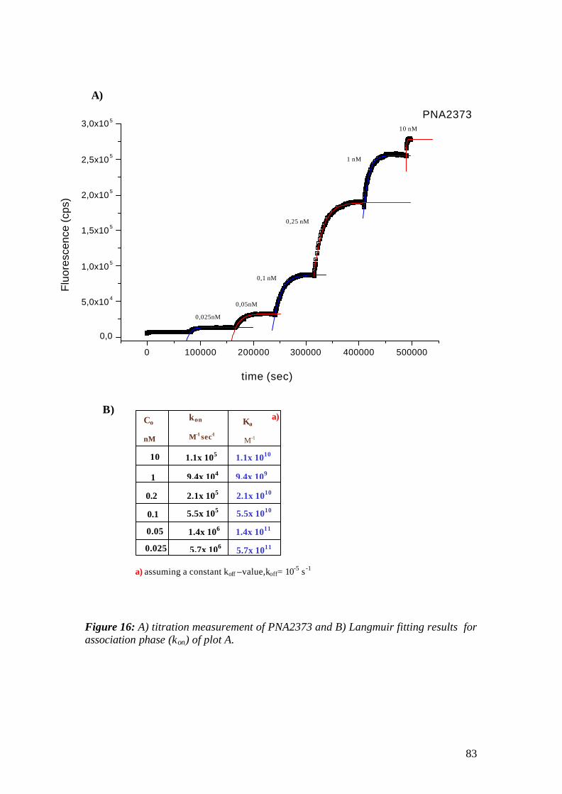
83
Figure 16: A) titration measurement of PNA2373 and B) Langmuir fitting results for association phase (kon) of plot A.
0 100000 200000 300000 400000 500000
0,0
5,0x10 4
1,0x10 5
1,5x10 5
2,0x10 5
2,5x10 5
3,0x10 5
Flu
ores
cenc
e (c
ps)
time (sec)
PNA2373
0,05nM
0,1 nM
0,25 nM
1 nM
10 nM
0,025nM
5.5x 10¹⁰
Ka
M-1
kon
M-1 sec-1
Co
nM
10
0.25
0.05
0.025
1.1x 10⁵ 1.1x 10¹⁰
9.4x 10⁴ 9.4x 10⁹
2.1x 10⁵ 2.1x 10¹⁰
1.4x 10⁶ 1.4x 10¹¹
5.7x 10¹¹ 5.7x 10⁶
1
0.1 5.5x 10⁵
a)
a) assuming a constant koff –value,koff= 10-5 s -1
A)
B)

84
Figure 17 : Titration measurement of PNA2370 and summary of the kon, koff values from the fitting of plot A and calculated affinity constant from kon/koff
The results from both titration measurements, i.e., based on saturation levels (Isat)
and on the max. intensity from the scan measurements, are summarized in Table 3.
Table 3: Affinity constant and half saturation value obtained from titration measurement for all PNAs
PNA name
Ka (M-1)
Kd (pM)
Ka (M-1)
Kd (pM) 2361 4x10
9 250 2.5 x10
9 400
2364 1.1x10¹⁰
92 1x10⁹ 1000
2367 1.3x10¹⁰
76 2.5x10¹⁰
40
2370 2.9x10⁹ 350 3x10
10 330
2373 5.6x10
9 180 5.9x10
9 170
2376 1.5x10
9 660 1.9x10
9 530
2379 1x10
9 1000 1x10
9 1000
The affinity constants obtained from the saturation values and the angular scans
show slight differences most likely as result of bulk contribution. If we looked again
back to the experimental procedure, the rinsing step starts right before the angular
From saturation value (Isat) From angular scan curves (Imax)
0 50000 100000 150000 200000 250000 300000-2,0x10⁴
0,0
2,0x10⁴
4,0x10⁴
6,0x10⁴
8,0x10⁴
1,0x10⁵
1,2x10⁵
1,4x10⁵
1,6x10⁵
1,8x10⁵
2,0x10⁵F
luor
esce
nce
(cps
)
time (sec)
PNA2370 all concentrations till 10nM
1
koff
sec-1
Ka
M-1
kon
M-1
sec-1
Co
nM
10
0,5
0,22
0,1
6.3x 10⁻⁶ 4.6x 10⁴ 7.3x 10⁹
7.14x 10 -6 1.3x 10⁵ 1.8x 10¹⁰
5.5x 10 -6 2.15x 10⁵ 3.9x 10¹⁰
6.3x 10 -6 6.4x 10⁵ 1x 10¹¹
6.3x 10 -6 3.2x 10¹¹ 2x 10⁶
0,1nM
0,22 nM
0,5 nM
1 nM
10 nM
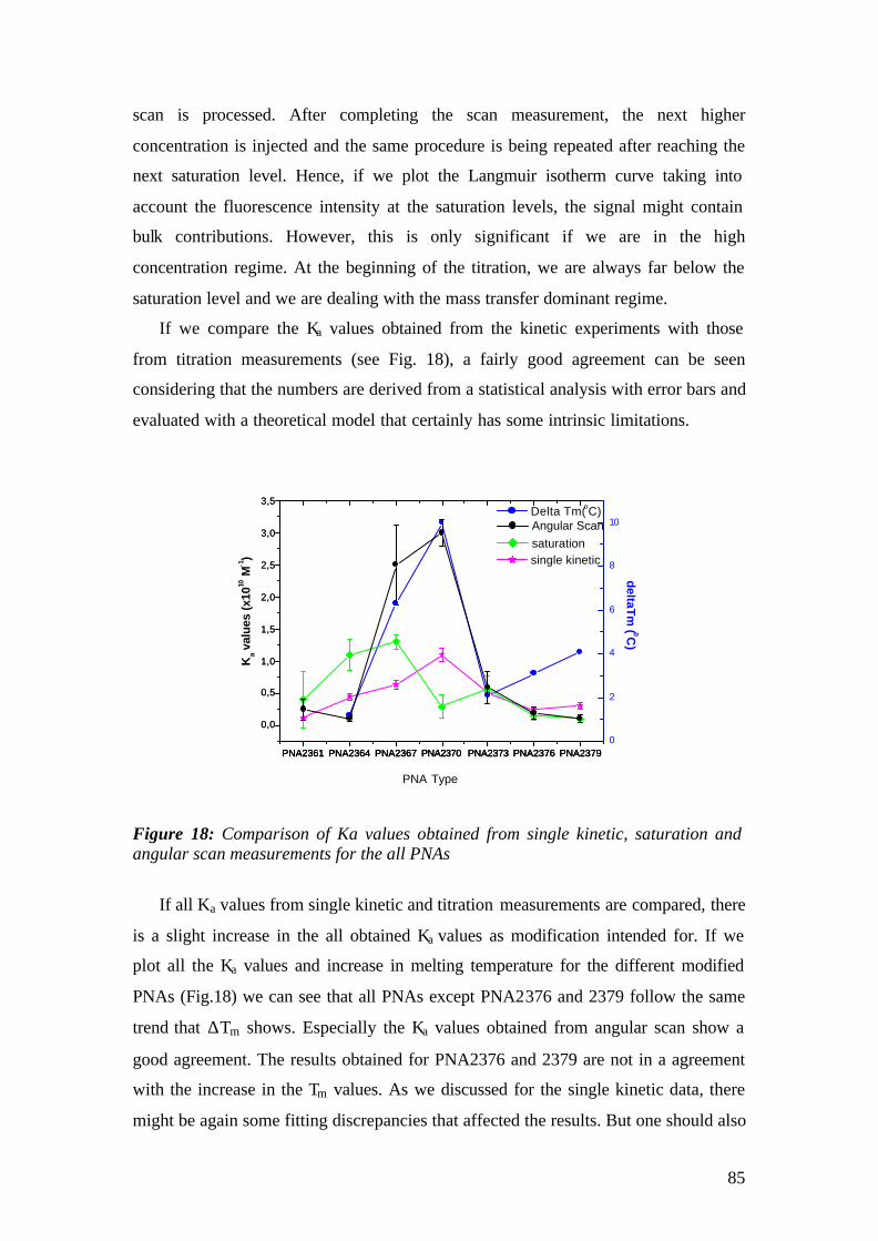
85
scan is processed. After completing the scan measurement, the next higher
concentration is injected and the same procedure is being repeated after reaching the
next saturation level. Hence, if we plot the Langmuir isotherm curve taking into
account the fluorescence intensity at the saturation levels, the signal might contain
bulk contributions. However, this is only significant if we are in the high
concentration regime. At the beginning of the titration, we are always far below the
saturation level and we are dealing with the mass transfer dominant regime.
If we compare the Ka values obtained from the kinetic experiments with those
from titration measurements (see Fig. 18), a fairly good agreement can be seen
considering that the numbers are derived from a statistical analysis with error bars and
evaluated with a theoretical model that certainly has some intrinsic limitations.
PNA2361 PNA2364 PNA2367 PNA2370 PNA2373 PNA2376 PNA2379
single kinetic
PNA Type
Ka v
alue
s (x
1010
M-1)
0
2
4
6
8
10 Delta Tm(oC)
deltaT
m ( 0C
)
PNA2361 PNA2364 PNA2367 PNA2370 PNA2373 PNA2376 PNA2379
0,0
0,5
1,0
1,5
2,0
2,5
3,0
3,5
saturation
PNA2361 PNA2364 PNA2367 PNA2370 PNA2373 PNA2376 PNA2379
0,0
0,5
1,0
1,5
2,0
2,5
3,0
3,5
Angular Scan
Figure 18: Comparison of Ka values obtained from single kinetic, saturation and angular scan measurements for the all PNAs
If all Ka values from single kinetic and titration measurements are compared, there
is a slight increase in the all obtained Ka values as modification intended for. If we
plot all the Ka values and increase in melting temperature for the different modified
PNAs (Fig.18) we can see that all PNAs except PNA2376 and 2379 follow the same
trend that ∆Tm shows. Especially the Ka values obtained from angular scan show a
good agreement. The results obtained for PNA2376 and 2379 are not in a agreement
with the increase in the Tm values. As we discussed for the single kinetic data, there
might be again some fitting discrepancies that affected the results. But one should also
86
mentioned that the hybridization process is more complicated than described by the
Langmuir model and there might be additional features happening during the
hybridization that our technique is unable to detect.
Other possibility is that our probe matrix could be dense in terms of space per
strand thus causing cross talk. Unfortunately, experiments with the diluted matrix
haven´t been performed. However, the diluted matrix affect has been studied by Dr.
Yao in the group in her PhD thesis and reduced cross talk between the neighboring
strands was observed.
Another fact related with the titration measurement is surface charges. After the
first concentration, the surface become occupied by target DNAs which bring
negative charges to the surface. If the next target concentration is injected, it has to
overcome this Coulombic barrier in order to find the probe strand. This makes the
binding process more complicated and might cause the disagreement with the
Langmuir model.
4.1.6 Global Analysis:
The Global analysis method is based on applying a non- linear least square
analysis and simultaneous fit to the association and disassociation phase data
generated for a range of DNA concentrations injected into the sample cell. This
method simply indicates that effects related to the probe surface, such as ionic
strength or bulk contribution, does not complicate the observed responses. Each
measurement is performed on a surface which is completely unoccupied by the target.
However, the affect of the regeneration of the surface should not be ignored.
How to do “Global fitting”:
1. Kinetic experiments are performed for ~5 concentrations (>half saturation), giving
10 minutes for the association, and 10 minutes for the dissociation (Fig.19) at a fixed
resonance angle for which the reflectivity is 30%;
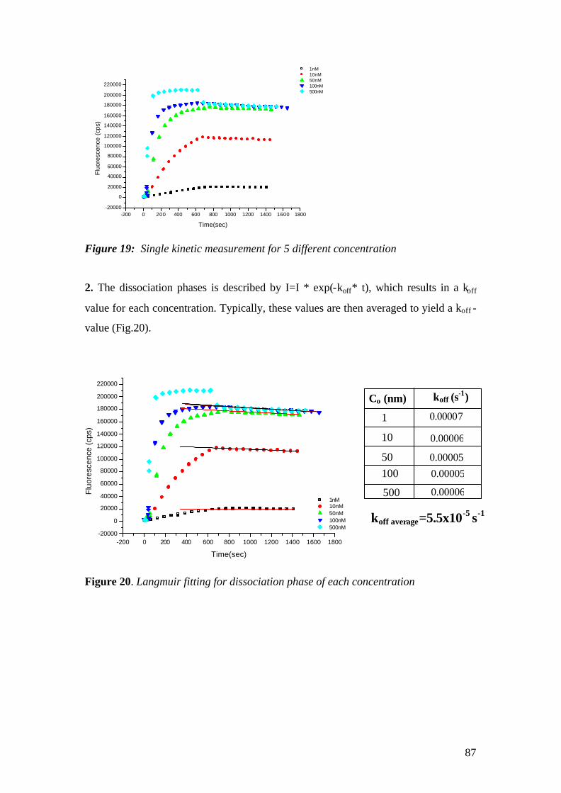
87
Figure 19: Single kinetic measurement for 5 different concentration
2. The dissociation phases is described by I=I * exp(-koff* t), which results in a koff
value for each concentration. Typically, these values are then averaged to yield a koff -
value (Fig.20).
Figure 20. Langmuir fitting for dissociation phase of each concentration
-200 0 200 400 600 800 1000 1200 1400 1600 1800-20000
0
20000
40000
60000
80000
100000
120000
140000
160000
180000
200000
220000
Flu
ores
cenc
e (c
ps)
Time(sec)
1nM 10nM 50nM 100nM 500nM
koff (s-1) Co (nm)
1
10
50 100
500
0.00005
0.00007
0.00006
0.00005
0.00006
koff average=5.5x10⁻⁵ s-1
-200 0 200 400 600 800 1000 1200 1400 1600 1800-20000
0
20000
40000
60000
80000
100000
120000
140000
160000
180000
200000
220000
Fluo
resc
ence
(cp
s)
Time(sec)
1nM 10nM 50nM 100nM 500nM
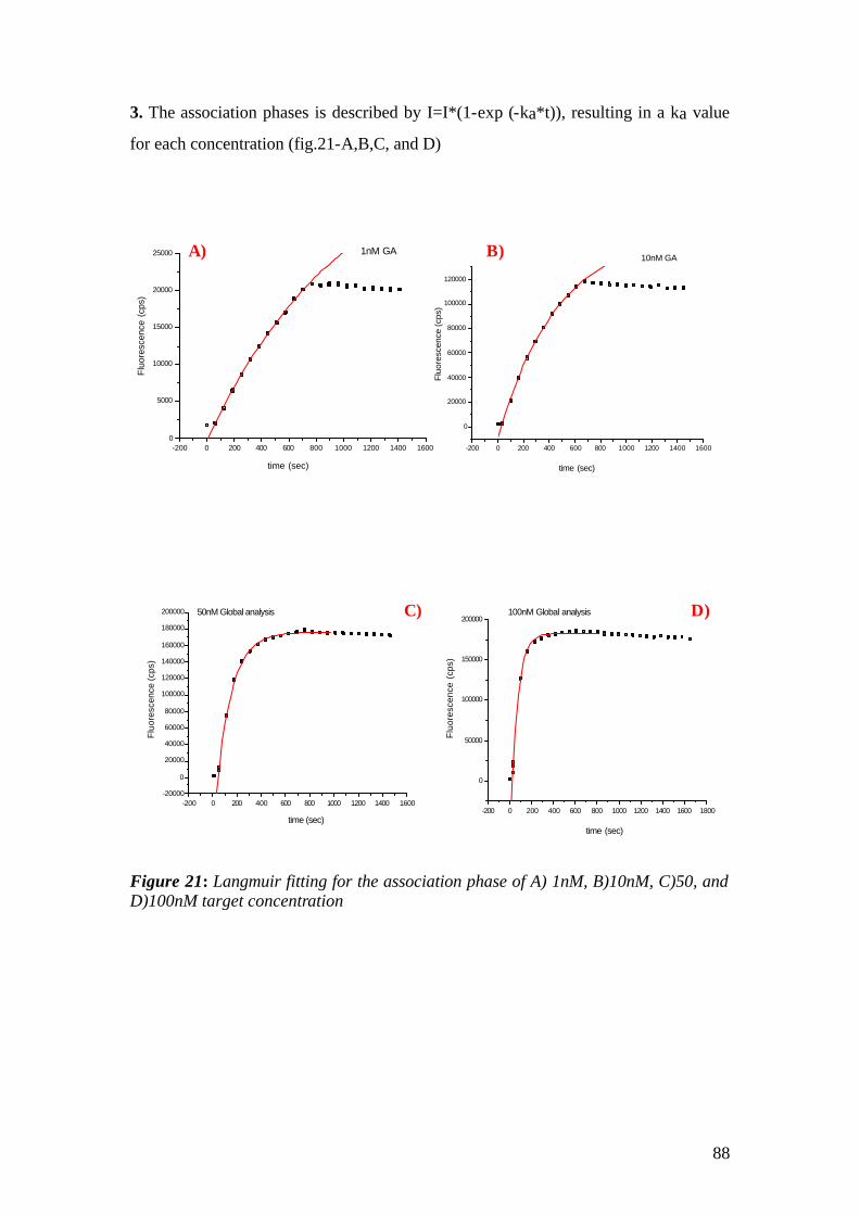
88
3. The association phases is described by I=I*(1-exp (-ka*t)), resulting in a ka value
for each concentration (fig.21-A,B,C, and D)
Figure 21: Langmuir fitting for the association phase of A) 1nM, B)10nM, C)50, and D)100nM target concentration
-200 0 200 400 600 800 1000 1200 1400 16000
5000
10000
15000
20000
25000
Flu
ores
cenc
e (c
ps)
time (sec)
1nM GA
-200 0 200 400 600 800 1000 1200 1400 1600
0
20000
40000
60000
80000
100000
120000
Flu
ores
cenc
e (c
ps)
time (sec)
10nM GAA) B)
-200 0 200 400 600 800 1000 1200 1400 1600-20000
0
20000
40000
60000
80000
100000
120000
140000
160000
180000
200000
Flu
ores
cenc
e (c
ps)
time (sec)
50nM Global analysis
-200 0 200 400 600 800 1000 1200 1400 1600 1800
0
50000
100000
150000
200000
Flu
ores
cenc
e (c
ps)
time (sec)
100nM Global analysisC) D)
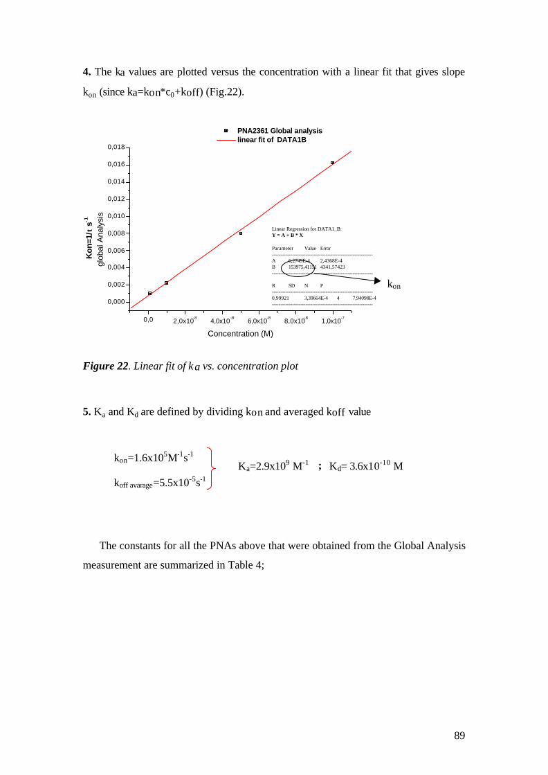
89
4. The ka values are plotted versus the concentration with a linear fit that gives slope
kon (since ka=kon*c0+koff) (Fig.22).
Figure 22. Linear fit of ka vs. concentration plot
5. Ka and Kd are defined by dividing kon and averaged koff value
The constants for all the PNAs above that were obtained from the Global Analysis
measurement are summarized in Table 4;
0,0 2,0x10⁻⁸
4,0x10⁻⁸
6,0x10⁻⁸
8,0x10⁻⁸
1,0x10⁻⁷
0,000
0,002
0,004
0,006
0,008
0,010
0,012
0,014
0,016
0,018
Kon
=1/τ
s-1
glob
al A
naly
sis
Linear Regression for DATA1_B:Y = A + B * X
Parameter Value Error------------------------------------------------------------A 6,2749E-4 2,4368E-4B 153975,41151 4341,57423------------------------------------------------------------
R SD N P------------------------------------------------------------0,99921 3,39664E-4 4 7,94098E-4------------------------------------------------------------
Concentration (M)
PNA2361 Global analysis linear fit of DATA1B
kon
kon=1.6x10⁵M-1s-1
koff avarage=5.5x10⁻⁵s-1
Ka=2.9x10⁹ M-1 Kd= 3.6x10⁻¹⁰ M ;

90
Table 4: Summary of the values that were obtained from Global Analysis for each
PNA
PNA name kon (M-1s-1) koff,avarage (s-1) Ka (M-1) Kd (pM)
2361 1.6x10⁵ 5.5x10⁻⁵ 2.9x10⁹ 360 2364
4.5x10⁴
2.6x10⁻⁵ 1.7x10⁹ 580
2367
7.7x10⁴ 4.5x10⁻⁵ 1.7x10⁹ 580
2370 5x10⁴ 3.4x10⁻⁵
1.5x10⁹ 680
2373
4.5x10⁴
2.8x10⁻⁵ 1.6x10⁹ 622
2376
2.4x10⁴ 6x10⁻⁵
4x10⁸ 2500
2379 2.1x10⁴ 8x10⁻⁵ 2.6x10⁸ 3800
If we compare the association constant obtained from the single kinetic
measurements with those from GA as plotted in Fig.23, a good correlation is being
observed, with a exception of PNA2361. For this system, the association constant
from the single measurement is almost an order of magnitude smaller than the one
obtained from the global analysis. However, the affinity constants, from two
measurements, are in the same order of magnitude.
PNA2361 PNA2364 PNA2367 PNA2370 PNA2373 PNA2376 PNA23790,0
0,5
1,0
1,5
2,0
sing
le k
on (x
105 M
-1s-1
)
from single kinetic from Global Analysis
PNA Type
Figure 23: Comparison of association constant, kon, obtained from Single Kinetic measurement and Global Analysis

91
We can do the same comparison for the affinity constants obtained from two
measurements. As we have seen in Fig.23, the association constant differs in some
cases, hence the Ka value will be effected. As can be seen in Fig.24 again, almost an
order of magnitude difference is observed. It is also clear that there is no correlation
between the affinity constants values which were obtained from single kinetic and
global analysis measurement. But if we reconsider the kon and koff values for two
measurements, one can see that the main difference comes from the dissociation rate
constant values. Since a fully complementary target is used, hence rather stable
duplexes are formed, 10min. rinsing phase is not sufficient to see significant
dissociation that can be analysed quantitatively.
PNA2361 PNA2364 PNA2367 PNA2370 PNA2373 PNA2376 PNA2379
0,0
0,5
1,0
1,5
2,0
2,5
3,0
Ka
from
sin
gle
kine
tic (
x101
0 M-1)
PNA Type
single kinetic
0,0
0,5
1,0
1,5
2,0
2,5
3,0
Ka from
Globa A
nalyses (x109 M
-1)
global analysis
Figure 24: Comparison of the affinity constants, Ka, obtained from Single Kinetic measurement and from Global Analysis
If we plot the ∆Tm and the Ka values for each PNA, as is done in Fig.25, no
correlation is observed.

92
PNA2361 PNA2364 PNA2367 PNA2370 PNA2373 PNA2376 PNA23790,0
0,5
1,0
1,5
2,0
2,5
3,0
Ka G
loba
l Ana
lysi
s(x1
09 M
-1)
PNA Type
Ka from Global Analysis
0
2
4
6
8
10
Delta Tm (Co)
delta Tm
(Co)
Figure 25: Ka from Global Analysis vs. ∆Tm
But if we have a close look to the overall picture in Fig.26 and plot all the Ka
values that we obtained from the 4 different calculations and compare them to the
difference in Tm, we can see that the increase in the change of Ka values only get
closer to the change in Tm values when we use the angular scan values while the
lowest Ka values were obtained with the global analysis method.
Figure 26: Plotting of Ka values obtained from Single kinetic, both Saturation and angular scan from titration measurements and Global Analysis measurement vs. ∆Tm
PNA2361 PNA2364 PNA2367 PNA2370 PNA2373 PNA2376 PNA23790,00,20,40,60,81,01,21,41,61,82,02,22,42,62,83,03,23,43,6
delta Tm
Ka (
M-1)x
1010
PNA Type
single kinetic
PNA2361 PNA2364 PNA2367 PNA2370 PNA2373 PNA2376 PNA23790,00,20,40,60,81,01,21,41,61,82,02,22,42,62,83,03,23,43,6
titration-saturation
PNA2361 PNA2364 PNA2367 PNA2370 PNA2373 PNA2376 PNA2379
0,20,40,60,81,01,21,41,61,82,02,22,42,62,83,03,23,43,6
titration scan
PNA2361 PNA2364 PNA2367 PNA2370 PNA2373 PNA2376 PNA23790,00,20,40,60,81,01,21,41,61,82,02,22,42,62,83,03,23,43,6
global analysis
0
2
4
6
8
10
delta Tm

93
As a conclusion, we can say that the PNA-DNA binding process is more
complicated than described by simple Langmuir model. Even though the bulk melting
temperature of the PNAs shows a correlation upon modification, PNAs behaves
differently when they are bound to the surface and the hybridization phenomenon
does not follow the simple Langmuirian behavior most of the time.
Molecular dynamic simulations [Sotiva et al,2000] indicate that the highly flexible
nature of the PNA backbone imposes energy penalties during the hybridization
interaction. The flexible nature of the PNA backbone makes it difficult for the
approaching DNA targets to relocate the recognition sites as compared to the DNA-
DNA hybridization interaction, where the charged nature of the DNA makes the
catcher probes stretched and thus, makes them easier accessible for the targets.
Another possibility is that there might be structural changes that are occurring during
the hybridization process. PNA is still a synthetic molecule that has a different
structure compared to DNA. Orozco and co-workers [Orozco et al.1998] state in their
studies that PNA molecules are not flexible enough that they can fit into any
oligonucleotide counterpart, and its interaction with DNA requires some
conformational changes. They have also shown that the internal energy of the PNA
backbone results in the distortion of the DNA backbone during the hybridization
process and they also emphasized that PNA demands a major change in the less
flexible DNA backbone. Normally during the DNA-DNA hybridization, the basic
structure of the individual DNA strands are altered via puckering of sugar units and
backbone stretching beside the recognition sequence affinity [Zubay et al.1995]. Even
though all those studies are performed in solution where the degrees of freedom are
much higher than on our restricted surface, the natural tendency for changing
conformation during the hybridization event might be more pronounced in our system
resulting with a deviation from the Langmuir behavior. However that limitation could
be avoided by using 3D dextran matrix in the future.
94
4.2 Surface Plasmon Fluorescence Microscopy (SPFM) studies of
PNA-DNA interaction on microarrays
4.2.1 Aim
The aim of this study is to investigate PNA-DNA hybridization with the materials
that have been discussed in chapter 4.1, using SPFM technique on an array platform.
We obtain the affinity constants, and investigate the correlation of Ka values with the
ones that were obtained from SPFS and Tm values. Since different PNAs have
different binding affinities to the same target, that should result in a SPFM experiment
in different intensity levels.
The materials are summarized in Table1 below as a remainder. The red color
letters represents the modifications that have been included in the backbone for
reasons that have been discussed in the chapter mentioned above. The code names are
given to the PNAs to simplify the names on the array according to the well numbers
that they were spotted to.
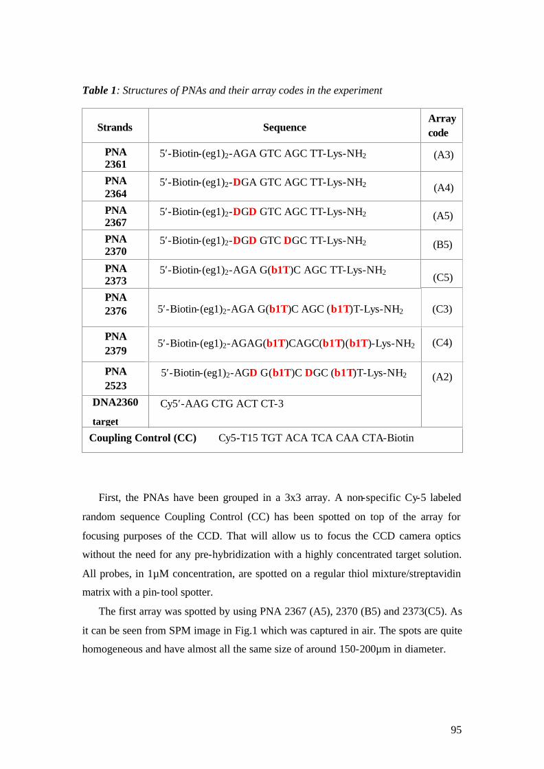
95
Table 1: Structures of PNAs and their array codes in the experiment
First, the PNAs have been grouped in a 3x3 array. A non-specific Cy-5 labeled
random sequence Coupling Control (CC) has been spotted on top of the array for
focusing purposes of the CCD. That will allow us to focus the CCD camera optics
without the need for any pre-hybridization with a highly concentrated target solution.
All probes, in 1µM concentration, are spotted on a regular thiol mixture/streptavidin
matrix with a pin- tool spotter.
The first array was spotted by using PNA 2367 (A5), 2370 (B5) and 2373(C5). As
it can be seen from SPM image in Fig.1 which was captured in air. The spots are quite
homogeneous and have almost all the same size of around 150-200µm in diameter.
(A2)
Strands
Sequence
PNA 2361
5′-Biotin-(eg1)2-AGA GTC AGC TT-Lys-NH2
PNA 2364
5′-Biotin-(eg1)2-DGA GTC AGC TT-Lys-NH2
PNA 2367
5′-Biotin-(eg1)2-DGD GTC AGC TT-Lys-NH2
PNA 2370
5′-Biotin-(eg1)2-DGD GTC DGC TT-Lys-NH2
PNA 2373
5′-Biotin-(eg1)2-AGA G(b1T)C AGC TT-Lys-NH2
PNA 2376
5′-Biotin-(eg1)2-AGA G(b1T)C AGC (b1T)T-Lys-NH2
PNA 2379
5′-Biotin-(eg1)2-AGAG(b1T)CAGC(b1T)(b1T)-Lys-NH2
DNA2360
target
Cy5′-AAG CTG ACT CT-3
Array code
(A3)
(A4)
(A5)
(B5)
(C5)
(C3)
(C4)
Coupling Control (CC) Cy5-T15 TGT ACA TCA CAA CTA-Biotin
PNA 2523
5′-Biotin-(eg1)2-AGD G(b1T)C DGC (b1T)T-Lys-NH2

96
In solution the array becomes invisible in SPM due to the low contrast. However,
a scan measurement was always done with SPM performed to determine the
resonance angle.
Figure 1: SPM image of Array 2A @ different resonance angle
Then the goniometer was tuned to θres and an interference filter was inserted in
front of the CCD camera in order to capture for fluorescence image. First the
background image with/without shutter open was captured as a reference that could be
subtracted from the actual images. Fig.2-A shows the background image, which is
captured with the laser blocked. The upper bright part of the image is back
illumination of the CCD sensor. Then the shutter was opened, the laser illuminated to
the sample and a background image was captured before any target injected. Fig.2-B
below shows the fluorescence image without any target hybridized. Only fluorescence
can be observed from the coupling control (CC) that was spotted for that purpose. The
acquisition time for the images was 30sec.
A) B)
C5 B5 A5
CC
500µm
3.5-4 mm
Figure 2: A) Background image B) SPFM image before any target injected
CC A) B)
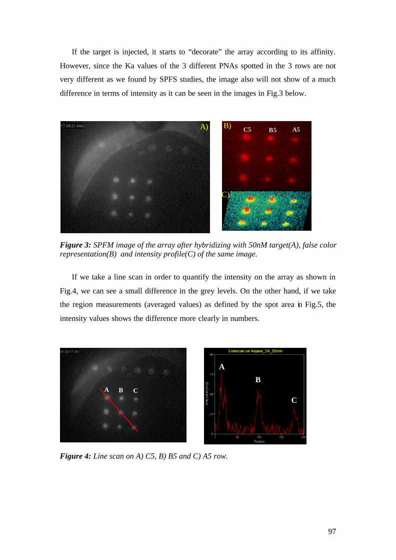
97
If the target is injected, it starts to “decorate” the array according to its affinity.
However, since the Ka values of the 3 different PNAs spotted in the 3 rows are not
very different as we found by SPFS studies, the image also will not show of a much
difference in terms of intensity as it can be seen in the images in Fig.3 below.
Figure 3: SPFM image of the array after hybridizing with 50nM target(A), false color representation(B) and intensity profile(C) of the same image.
If we take a line scan in order to quantify the intensity on the array as shown in
Fig.4, we can see a small difference in the grey levels. On the other hand, if we take
the region measurements (averaged values) as defined by the spot area in Fig.5, the
intensity values shows the difference more clearly in numbers.
Figure 4: Line scan on A) C5, B) B5 and C) A5 row.
C5 B5 A5 A) B)
C)
A
B
C A B C
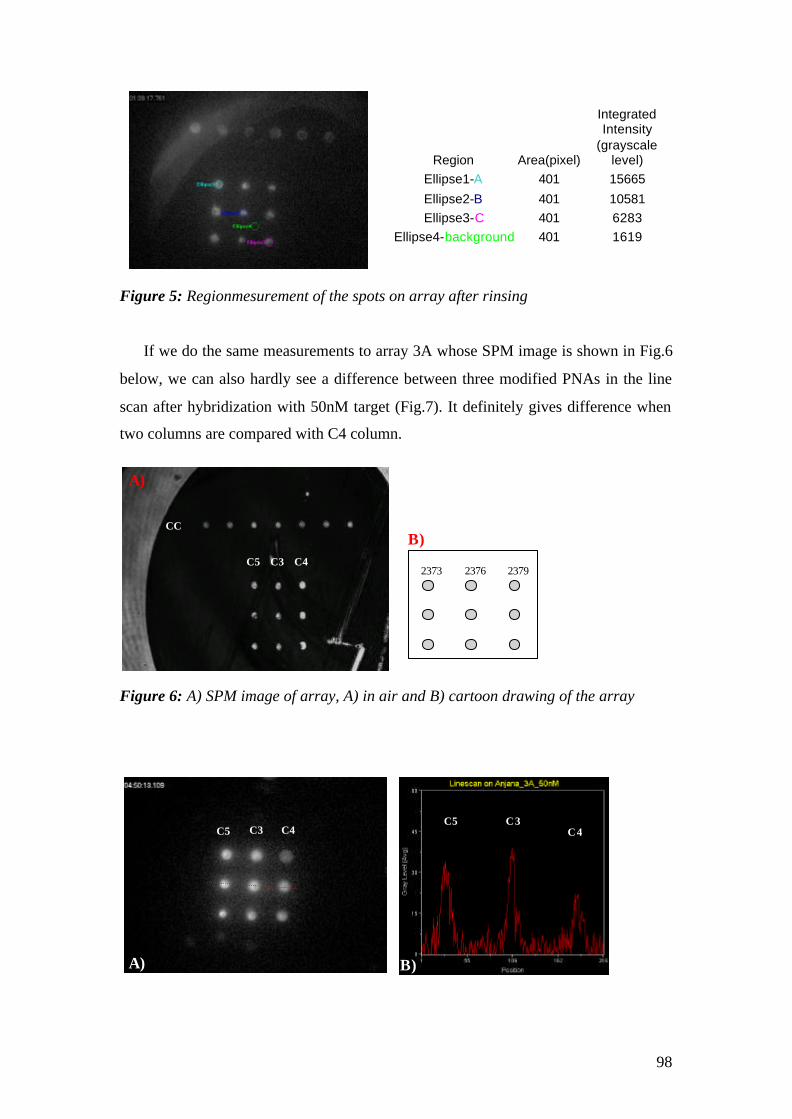
98
Figure 5: Regionmesurement of the spots on array after rinsing
If we do the same measurements to array 3A whose SPM image is shown in Fig.6
below, we can also hardly see a difference between three modified PNAs in the line
scan after hybridization with 50nM target (Fig.7). It definitely gives difference when
two columns are compared with C4 column.
Figure 6: A) SPM image of array, A) in air and B) cartoon drawing of the array
Region Area(pixel)
Integrated Intensity
(grayscale level)
Ellipse1-A 401 15665
Ellipse2-B 401 10581 Ellipse3-C 401 6283
Ellipse4-background 401 1619
C3 C5 C4 C3 C5
C4
A) B)
2373 2376 2379
A)
B) C3 C5 C4
CC
A)
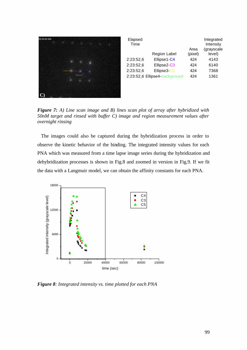
99
Elapsed Time
Region Label Area
(pixel)
Integrated Intensity
(grayscale level)
2:23:52,6 Ellipse1-C4 424 4143 2:23:52,6 Ellipse2-C3 424 6140 2:23:52,6 Ellipse3-C5 424 7368 2:23:52,6 Ellipse4-background 424 1361
Figure 7: A) Line scan image and B) lines scan plot of array after hybridized with 50nM target and rinsed with buffer C) image and region measurement values after overnight rinsing
The images could also be captured during the hybridization process in order to
observe the kinetic behavior of the binding. The integrated intensity values for each
PNA which was measured from a time lapse image series during the hybridization and
dehybridization processes is shown in Fig.8 and zoomed in version in Fig.9. If we fit
the data with a Langmuir model, we can obtain the affinity constants for each PNA.
0 20000 40000 60000 80000 1000000
6000
12000
18000
Inte
grat
ed in
tens
ity (g
rays
cale
leve
l)
time (sec)
C4 C3 C5
Figure 8: Integrated intensity vs. time plotted for each PNA
C)
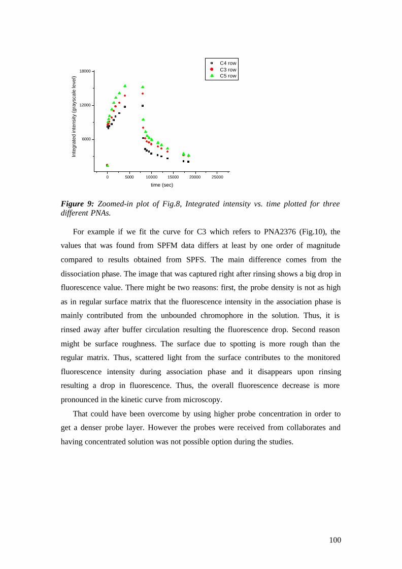
100
0 5000 10000 15000 20000 25000
6000
12000
18000In
tegr
ated
inte
nsity
(gra
ysca
le le
vel)
time (sec)
C4 row C3 row C5 row
Figure 9: Zoomed-in plot of Fig.8, Integrated intensity vs. time plotted for three different PNAs. For example if we fit the curve for C3 which refers to PNA2376 (Fig.10), the
values that was found from SPFM data differs at least by one order of magnitude
compared to results obtained from SPFS. The main difference comes from the
dissociation phase. The image that was captured right after rinsing shows a big drop in
fluorescence value. There might be two reasons: first, the probe density is not as high
as in regular surface matrix that the fluorescence intensity in the association phase is
mainly contributed from the unbounded chromophore in the solution. Thus, it is
rinsed away after buffer circulation resulting the fluorescence drop. Second reason
might be surface roughness. The surface due to spotting is more rough than the
regular matrix. Thus, scattered light from the surface contributes to the monitored
fluorescence intensity during association phase and it disappears upon rinsing
resulting a drop in fluorescence. Thus, the overall fluorescence decrease is more
pronounced in the kinetic curve from microscopy.
That could have been overcome by using higher probe concentration in order to
get a denser probe layer. However the probes were received from collaborates and
having concentrated solution was not possible option during the studies.
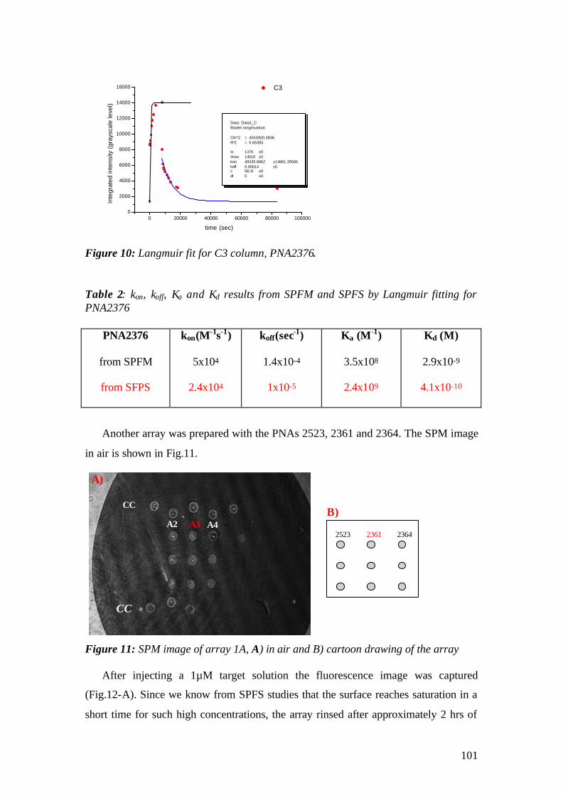
101
Figure 10: Langmuir fit for C3 column, PNA2376. Table 2: kon, koff, Ka and Kd results from SPFM and SPFS by Langmuir fitting for PNA2376
Another array was prepared with the PNAs 2523, 2361 and 2364. The SPM image
in air is shown in Fig.11.
Figure 11: SPM image of array 1A, A) in air and B) cartoon drawing of the array After injecting a 1µM target solution the fluorescence image was captured
(Fig.12-A). Since we know from SPFS studies that the surface reaches saturation in a
short time for such high concentrations, the array rinsed after approximately 2 hrs of
PNA2376
from SPFM
from SFPS
kon(M-1s-1)
5x10⁴
2.4x10⁴
koff(sec-1)
1.4x10⁻⁴
1x10⁻⁵
Ka (M-1)
3.5x10⁸
2.4x10⁹
Kd (M)
2.9x10⁻⁹
4.1x10⁻¹⁰
0 20000 40000 60000 80000 1000000
2000
4000
6000
8000
10000
12000
14000
16000
Data: Data1_CModel: langmuirkon Chi^2 = 4553920.3836R 2 = 0.65393 Io 1376 ±0Imax 14010 ±0kon 49335.8862 ±14881.35506koff 0.00014 ±0c 5E-8 ±0dt 0 ±0
Inte
grat
ed in
tens
ity (
gray
scal
e le
vel)
time (sec)
C3
A4 A3 A2
CC
CC
2523 2361 2364
A)
B)
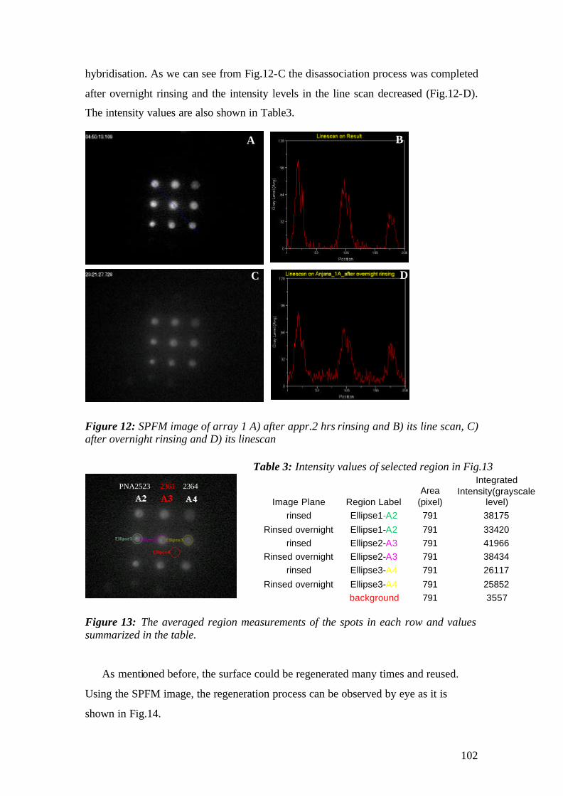
102
hybridisation. As we can see from Fig.12-C the disassociation process was completed
after overnight rinsing and the intensity levels in the line scan decreased (Fig.12-D).
The intensity values are also shown in Table3.
Figure 12: SPFM image of array 1 A) after appr.2 hrs rinsing and B) its line scan, C) after overnight rinsing and D) its linescan
Figure 13: The averaged region measurements of the spots in each row and values summarized in the table.
As mentioned before, the surface could be regenerated many times and reused.
Using the SPFM image, the regeneration process can be observed by eye as it is
shown in Fig.14.
Image Plane Region Label Area
(pixel)
Integrated Intensity(grayscale
level) rinsed Ellipse1-A2 791 38175
Rinsed overnight Ellipse1-A2 791 33420 rinsed Ellipse2-A3 791 41966
Rinsed overnight Ellipse2-A3 791 38434 rinsed Ellipse3-A4 791 26117
Rinsed overnight Ellipse3-A4 791 25852 background 791 3557
A B
C D
PNA2523 2361 2364
Table 3: Intensity values of selected region in Fig.13
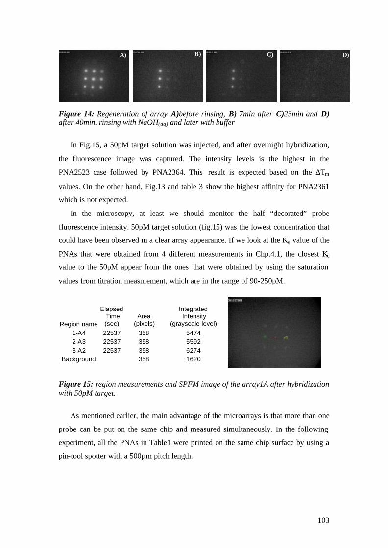
103
Figure 14: Regeneration of array A)before rinsing, B) 7min after C)23min and D) after 40min. rinsing with NaOH(aq) and later with buffer
In Fig.15, a 50pM target solution was injected, and after overnight hybridization,
the fluorescence image was captured. The intensity levels is the highest in the
PNA2523 case followed by PNA2364. This result is expected based on the ∆Tm
values. On the other hand, Fig.13 and table 3 show the highest affinity for PNA2361
which is not expected.
In the microscopy, at least we should monitor the half “decorated” probe
fluorescence intensity. 50pM target solution (fig.15) was the lowest concentration that
could have been observed in a clear array appearance. If we look at the Ka value of the
PNAs that were obtained from 4 different measurements in Chp.4.1, the closest Kd
value to the 50pM appear from the ones that were obtained by using the saturation
values from titration measurement, which are in the range of 90-250pM.
Figure 15: region measurements and SPFM image of the array1A after hybridization with 50pM target.
As mentioned earlier, the main advantage of the microarrays is that more than one
probe can be put on the same chip and measured simultaneously. In the following
experiment, all the PNAs in Table1 were printed on the same chip surface by using a
pin-tool spotter with a 500µm pitch length.
Region name
Elapsed Time (sec)
Area (pixels)
Integrated Intensity
(grayscale level) 1-A4 22537 358 5474 2-A3 22537 358 5592 3-A2 22537 358 6274
Background 358 1620
A) B) C) D)
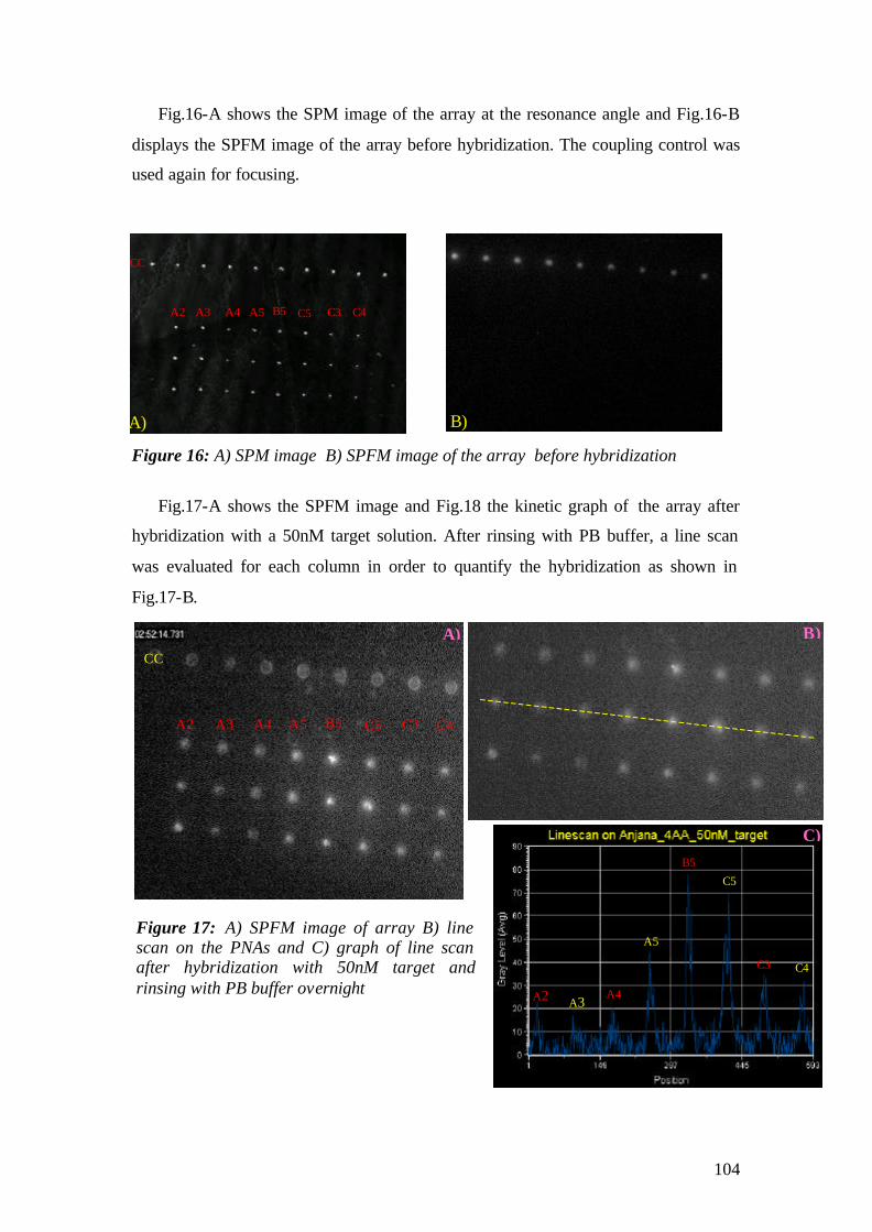
104
Fig.16-A shows the SPM image of the array at the resonance angle and Fig.16-B
displays the SPFM image of the array before hybridization. The coupling control was
used again for focusing.
Figure 16: A) SPM image B) SPFM image of the array before hybridization
Fig.17-A shows the SPFM image and Fig.18 the kinetic graph of the array after
hybridization with a 50nM target solution. After rinsing with PB buffer, a line scan
was evaluated for each column in order to quantify the hybridization as shown in
Fig.17-B.
Fig.17-B and 17-C.
Figure 17: A) SPFM image of array B) line scan on the PNAs and C) graph of line scan after hybridization with 50nM target and rinsing with PB buffer overnight
A) B)
A2 A3 A4
A5
B5
C5
C3 C4
C)
A2 A3 A4 A5 B5 C5 C3 C4
CC
A) B)
CC
A2 A3 A4 A5 B5 C5 C3 C4
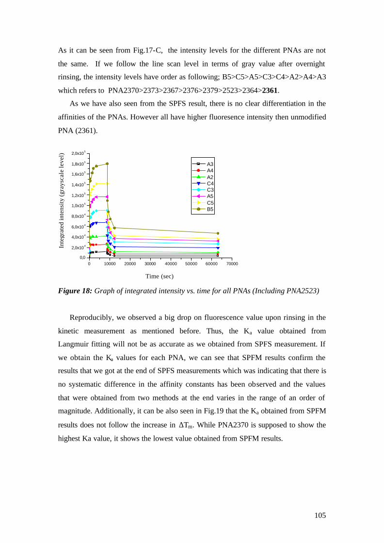
105
As it can be seen from Fig.17-C, the intensity levels for the different PNAs are not
the same. If we follow the line scan level in terms of gray value after overnight
rinsing, the intensity levels have order as following; B5>C5>A5>C3>C4>A2>A4>A3
which refers to PNA2370>2373>2367>2376>2379>2523>2364>2361.
As we have also seen from the SPFS result, there is no clear differentiation in the
affinities of the PNAs. However all have higher fluoresence intensity then unmodified
PNA (2361).
Figure 18: Graph of integrated intensity vs. time for all PNAs (Including PNA2523)
Reproducibly, we observed a big drop on fluorescence value upon rinsing in the
kinetic measurement as mentioned before. Thus, the Ka value obtained from
Langmuir fitting will not be as accurate as we obtained from SPFS measurement. If
we obtain the Ka values for each PNA, we can see that SPFM results confirm the
results that we got at the end of SPFS measurements which was indicating that there is
no systematic difference in the affinity constants has been observed and the values
that were obtained from two methods at the end varies in the range of an order of
magnitude. Additionally, it can be also seen in Fig.19 that the Ka obtained from SPFM
results does not follow the increase in ∆Tm. While PNA2370 is supposed to show the
highest Ka value, it shows the lowest value obtained from SPFM results.
0 10000 20000 30000 40000 50000 60000 700000,0
2,0x10⁴
4,0x10⁴
6,0x10⁴
8,0x10⁴
1,0x10⁵
1,2x10⁵
1,4x10⁵
1,6x10⁵
1,8x10⁵
2,0x10⁵
Inte
grat
ed in
tens
ity
time(sec)
A3 A4 A2 C4 C3 A5 C5 B5
Inte
grat
ed in
tens
ity (g
rays
cale
leve
l)
Time (sec)
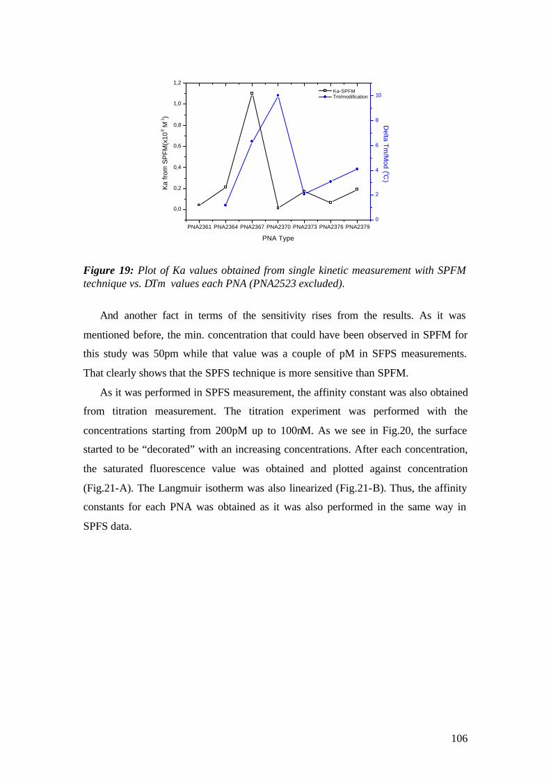
106
PNA2361 PNA2364 PNA2367 PNA2370 PNA2373 PNA2376 PNA2379
0,0
0,2
0,4
0,6
0,8
1,0
1,2 Ka-SPFM Tm/modification
PNA Type
Ka
from
SP
FM(x
108 M
-1)
0
2
4
6
8
10
Delta T
m/M
od ( oC)
Figure 19: Plot of Ka values obtained from single kinetic measurement with SPFM technique vs. ∆Tm values each PNA (PNA2523 excluded).
And another fact in terms of the sensitivity rises from the results. As it was
mentioned before, the min. concentration that could have been observed in SPFM for
this study was 50pm while that value was a couple of pM in SFPS measurements.
That clearly shows that the SPFS technique is more sensitive than SPFM.
As it was performed in SPFS measurement, the affinity constant was also obtained
from titration measurement. The titration experiment was performed with the
concentrations starting from 200pM up to 100nM. As we see in Fig.20, the surface
started to be “decorated” with an increasing concentrations. After each concentration,
the saturated fluorescence value was obtained and plotted against concentration
(Fig.21-A). The Langmuir isotherm was also linearized (Fig.21-B). Thus, the affinity
constants for each PNA was obtained as it was also performed in the same way in
SPFS data.
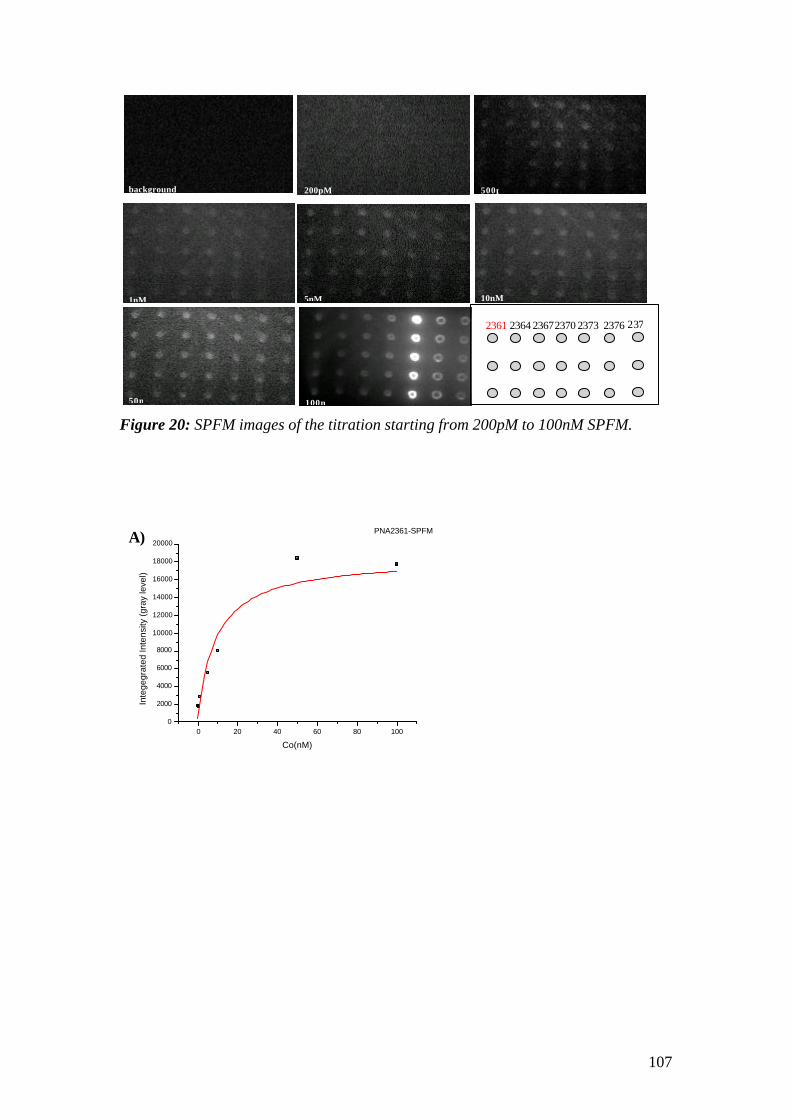
107
Figure 20: SPFM images of the titration starting from 200pM to 100nM SPFM.
0 20 40 60 80 1000
2000
4000
6000
8000
10000
12000
14000
16000
18000
20000
Inte
gegr
ated
Inte
nsity
(gra
y le
vel)
Co(nM)
PNA2361-SPFM
500p
5nM 1nM
50n
10nM
100n
background 200pM
2370 2373 2376 2361 2364 2367 2379
A)
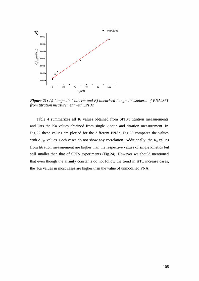
108
0 20 40 60 80 100
0,000
0,001
0,002
0,003
0,004
0,005
0,006C
0/I sat(n
M/a
.u)
C0(nM)
PNA2361
Figure 21: A) Langmuir Isotherm and B) linearized Langmuir isotherm of PNA2361 from titration measurement with SPFM
Table 4 summarizes all Ka values obtained from SPFM titration measurements
and lists the Ka values obtained from single kinetic and titration measurement. In
Fig.22 these values are plotted for the different PNAs. Fig.23 compares the values
with ∆Tm values. Both cases do not show any correlation. Additionally, the Ka values
from titration measurement are higher than the respective values of single kinetics but
still smaller than that of SPFS experiments (Fig.24). However we should mentioned
that even though the affinity constants do not follow the trend in ∆Tm increase cases,
the Ka values in most cases are higher than the value of unmodified PNA.
B)

109
Table 4: Affinity constanst and half saturation value obtained from single kinetic and titration measurement by SPFM for all PNAs
PNA2361 PNA2364 PNA2367 PNA2370 PNA2373 PNA2376 PNA2379
0
2
4
6
8
10
12
14
16
18
20
Ka from
SP
FM
single kinetic(x107 M
-1)K
a fr
om S
PF
M ti
trat
ion(
x107
M-1
)
PNA Type
SPFM titration
0
2
4
6
8
10
12
SPFM single kinetic
Figure 22: Ka values obtained from titration measurement and single kinetic measurements with SPFM for each PNA.
PNA name
Ka (M-1)
Kd (M)
Ka (M-1)
Kd (M) 2361 4.3 x10⁶
2.3 x10⁻⁷
1.1x10⁸
9.1 x10⁻⁹
2364 2.1 x10⁷ 4.8 x10⁻⁸ 1.1x10⁸ 9.1 x10⁻⁹
2367 1.1 x10⁸ 9.1 x10⁻⁹ 6.1x10⁷ 1.6 x10⁻⁸
2370 1.3 x10⁶ 7.7 x10⁻⁷ 3.6x10⁷ 9.1 x10⁻⁹
2373 1.7 x10⁷ 5.9 x10⁻⁸ 4.5x10⁷ 2.2 x10⁻⁸
2376 6.9 x10⁶ 1.5 x10⁻⁷ 6.6x10⁷ 1.5 x10⁻⁸
2379 1.9 x10⁷ 5.3x10⁻⁸ 3.5x10⁷ 2.9 x10⁻⁸
From single kinetic From saturation value (Isat)
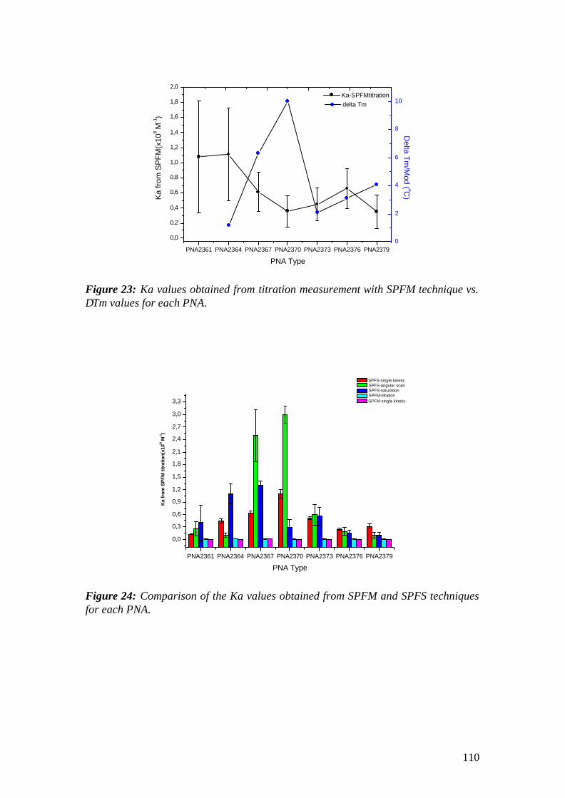
110
PNA2361 PNA2364 PNA2367 PNA2370 PNA2373 PNA2376 PNA2379
0,0
0,2
0,4
0,6
0,8
1,0
1,2
1,4
1,6
1,8
2,0
Delta T
m/M
od ( oC)K
a fr
om S
PF
M(x
108 M
-1)
PNA Type
Ka-SPFMtitration
0
2
4
6
8
10
delta Tm
Figure 23: Ka values obtained from titration measurement with SPFM technique vs. ∆Tm values for each PNA.
PNA2361 PNA2364 PNA2367 PNA2370 PNA2373 PNA2376 PNA2379
0,0
0,3
0,6
0,9
1,2
1,5
1,8
2,1
2,4
2,7
3,0
3,3
Ka
from
SP
FM t
itrat
ion(
x1010
M-1)
PNA Type
SPFS-single kinetic SPFS-angular scan SPFS-saturation SPFM-titration SPFM-single kinetic
Figure 24: Comparison of the Ka values obtained from SPFM and SPFS techniques for each PNA.
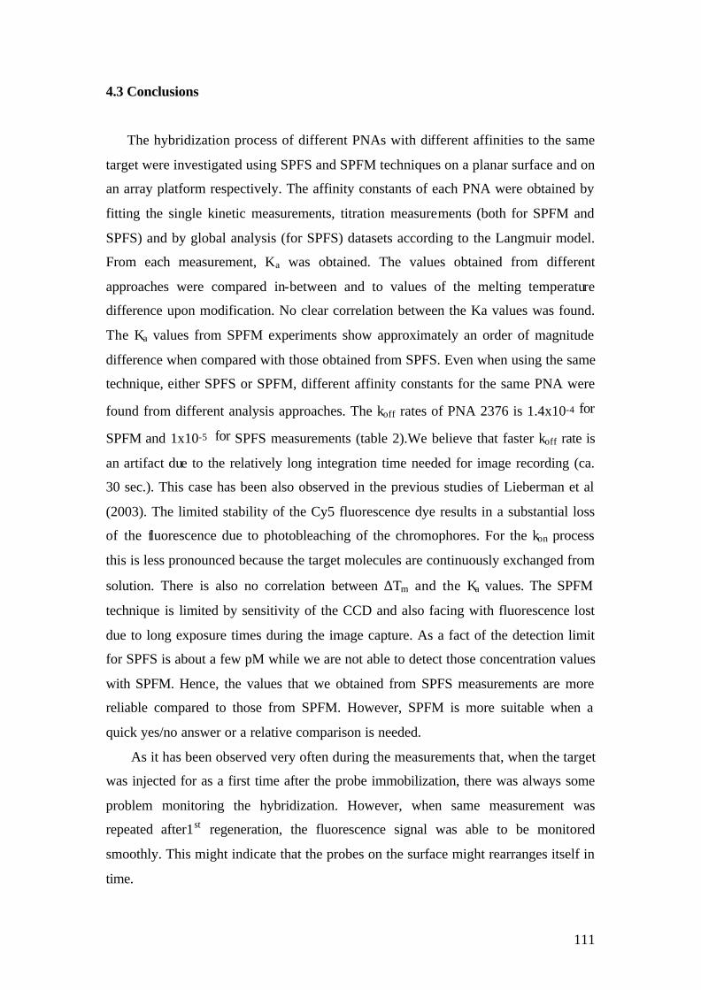
111
4.3 Conclusions
The hybridization process of different PNAs with different affinities to the same
target were investigated using SPFS and SPFM techniques on a planar surface and on
an array platform respectively. The affinity constants of each PNA were obtained by
fitting the single kinetic measurements, titration measurements (both for SPFM and
SPFS) and by global analysis (for SPFS) datasets according to the Langmuir model.
From each measurement, Ka was obtained. The values obtained from different
approaches were compared in-between and to values of the melting temperature
difference upon modification. No clear correlation between the Ka values was found.
The Ka values from SPFM experiments show approximately an order of magnitude
difference when compared with those obtained from SPFS. Even when using the same
technique, either SPFS or SPFM, different affinity constants for the same PNA were
found from different analysis approaches. The koff rates of PNA 2376 is 1.4x10⁻⁴ for
SPFM and 1x10⁻⁵ for SPFS measurements (table 2).We believe that faster koff rate is
an artifact due to the relatively long integration time needed for image recording (ca.
30 sec.). This case has been also observed in the previous studies of Lieberman et al
(2003). The limited stability of the Cy5 fluorescence dye results in a substantial loss
of the fluorescence due to photobleaching of the chromophores. For the kon process
this is less pronounced because the target molecules are continuously exchanged from
solution. There is also no correlation between ∆Tm and the Ka values. The SPFM
technique is limited by sensitivity of the CCD and also facing with fluorescence lost
due to long exposure times during the image capture. As a fact of the detection limit
for SPFS is about a few pM while we are not able to detect those concentration values
with SPFM. Hence, the values that we obtained from SPFS measurements are more
reliable compared to those from SPFM. However, SPFM is more suitable when a
quick yes/no answer or a relative comparison is needed.
As it has been observed very often during the measurements that, when the target
was injected for as a first time after the probe immobilization, there was always some
problem monitoring the hybridization. However, when same measurement was
repeated after1st regeneration, the fluorescence signal was able to be monitored
smoothly. This might indicate that the probes on the surface might rearranges itself in
time.

112
There were also no correlation observed between with ∆Tm values and the affinity
constants. ∆Tm values were measured by collaborators and they represent the stability
increase of the duplex PNA-DNA in solution. Since our technique is a surface
sensitive technique, the conformational change upon surface-immobilization might
effect the kinetic behavior of the PNAs resulting in the deviation in Ka values.
Addit ionally, as it was also mentioned earlier that the sharp decrease in the
fluorescence intensity upon rinsing as result of either low probe density or surface
roughness effects the dissociation curve. Thus, it gets very difficult to obtain a
meaningful Ka value out of a single kinetic measurement by SPFM.
113
5. Genetically Modified Organism (GMO) detection in food chain by
means of DNA-DNA and PNA-DNA Hybridization by Surface
Plasmon Fluorescence Spectorcopy (SPFM)
5.1 DNA-DNA Hybridization on a Biotin / Streptavidin Matrix
5.1.1 Aim
The presence of ingredients derived from GMOs in food production, in the market
is subject to number of European Regulations that stipulate which product consisting
of or containing GMO-derived ingredients should be labeled. In recent incidence,
according to reports [E.Kok et al,2002] where unapproved GMO varieties entered to EU
market played driving force role to develop more powerful tool for GMO detection
and identification in the food cha in in order to maintain this labeling requirements.
Our studies are very relevant since our approach can offer a sensitive method for
real-time analysis both a labelled and a non- labelled platform on an array bases. The
EU project (DNA-Track, OLK1-2000-01658) has the aim to detect GMO contents in the
food chain based on the DNA and PNA array technology. The collaborators are listed
in Appendix A. The limit for labelling which is 1% GMO content was the ultimate
aim of GMO detection in the food chain project and
This part of the study involves GMO detection based on a regular streptavidin
matrix as described in section. 3.2.1 and 3.2.2 by using a DNA probe and a DNA
target with 1 or 2 mismatches on the backbone.
The oligonucleotides that have been used as model system for spotting are shown
in Table 1. The biotinylated probes were obtained from MWG, Germany. The total
lengths of the probes are 30 bases with a 15mer T spacer and a specific 15mer
recognition sequence. The mismatches (MM) are placed in the middle of the
recognition sequence on the G base. For detection of GMOs, 2 kinds of amplicons
were prepared by polymerase chain reaction (PCR) method from natural soybean (SL)
and from genetically modified round-up ready soybean (RR) for detection of GMO.
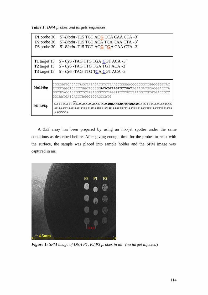
114
Table 1: DNA probes and targets sequences
A 3x3 array has been prepared by using an ink-jet spotter under the same
conditions as described before. After giving enough time for the probes to react with
the surface, the sample was placed into sample holder and the SPM image was
captured in air.
Figure 1: SPM image of DNA P1, P2,P3 probes in air- (no target injected)
P3 P1 P2
500µm
~ 4.5mm
P1 probe 30 5´-Biotin -T15 TGT ACG TCA CAA CTA -3´ P2 probe 30 5´-Biotin -T15 TGT ACA TCA CAA CTA -3´ P3 probe 30 5´-Biotin -T15 TGT ACG TGA CAA CTA -3´ T1 target 15 5´- Cy5 -TAG TTG TGA CGT ACA -3´ T2 target 15 5´- Cy5 -TAG TTG TGA TGT ACA -3´ T3 target 15 5´- Cy5 -TAG TTG TCA CGT ACA -3´
CGGCGGTCACACTACCTATAGACGTCTTAAGCGGGAACCCCGGGTCGGCCGGTTACTTGGTGGCTCCCCTGGCTCCCGGACATGTAGTGTTGATTGAAGATGCACGGACCTAGGCGCACCACTGGCTCTAGAGGGCCCTAGGTTCCCGCTTAAGGTCGTGTGACCGCCGGCAATGATCACCTAGGCTCGAGCCATG
Mu196bp
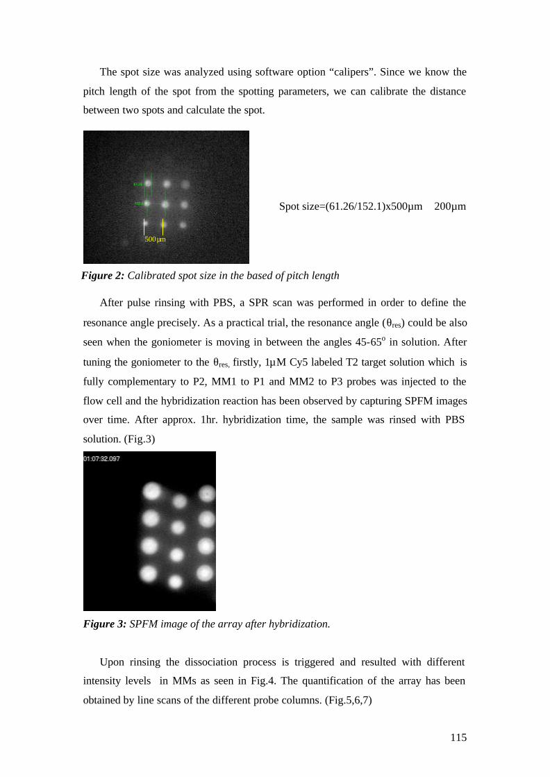
115
The spot size was analyzed using software option “calipers”. Since we know the
pitch length of the spot from the spotting parameters, we can calibrate the distance
between two spots and calculate the spot.
Spot size=(61.26/152.1)x500µm ≅ 200µm
After pulse rinsing with PBS, a SPR scan was performed in order to define the
resonance angle precisely. As a practical trial, the resonance angle (θres) could be also
seen when the goniometer is moving in between the angles 45-65o in solution. After
tuning the goniometer to the θres, firstly, 1µM Cy5 labeled T2 target solution which is
fully complementary to P2, MM1 to P1 and MM2 to P3 probes was injected to the
flow cell and the hybridization reaction has been observed by capturing SPFM images
over time. After approx. 1hr. hybridization time, the sample was rinsed with PBS
solution. (Fig.3)
Figure 3: SPFM image of the array after hybridization.
Upon rinsing the dissociation process is triggered and resulted with different
intensity levels in MMs as seen in Fig.4. The quantification of the array has been
obtained by line scans of the different probe columns. (Fig.5,6,7)
500µm
Figure 2: Calibrated spot size in the based of pitch length

116
Figure 4: SPFM picture of the array hybridized with 1µM T2 target and 13min. after rinsing with PBS.
Figure 5: Line scan of P2 row, which is MM0 for T2 target
Figure 6: Line scan of P1 row, which is MM1 for T2 target
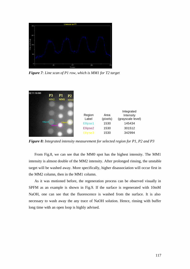
117
Figure 7: Line scan of P1 row, which is MM1 for T2 target
Figure 8: Integrated intensity measurement for selected region for P1, P2 and P3
From Fig.8, we can see that the MM0 spot has the highest intensity. The MM1
intensity is almost double of the MM2 intensity. After prolonged rinsing, the unstable
target will be washed away. More specifically, higher disassociation will occur first in
the MM2 column, then in the MM1 column.
As it was motioned before, the regeneration process can be observed visually in
SPFM as an example is shown in Fig.9. If the surface is regenerated with 10mM
NaOH, one can see that the fluorescence is washed from the surface. It is also
necessary to wash away the any trace of NaOH solution. Hence, rinsing with buffer
long time with an open loop is highly advised.
Region Label
Area (pixels)
Integrated Intensity
(grayscale level) Ellipse1 1530 145434
Ellipse2 1530 301512 Ellipse3 1530 342994
P3 MM2
P1 MM1
P2 MM0
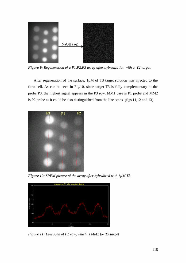
118
Figure 9: Regeneration of a P1,P2,P3 array after hybridization with a T2 target.
After regeneration of the surface, 1µM of T3 target solution was injected to the
flow cell. As can be seen in Fig.10, since target T3 is fully complementary to the
probe P3, the highest signal appears in the P3 row. MM1 case is P1 probe and MM2
is P2 probe as it could be also distinguished from the line scans (figs.11,12 and 13)
Figure 10: SPFM picture of the array after hybridized with 1µM T3
Figure 11: Line scan of P1 row, which is MM2 for T3 target
NaOH (aq)
P3 P1 P2
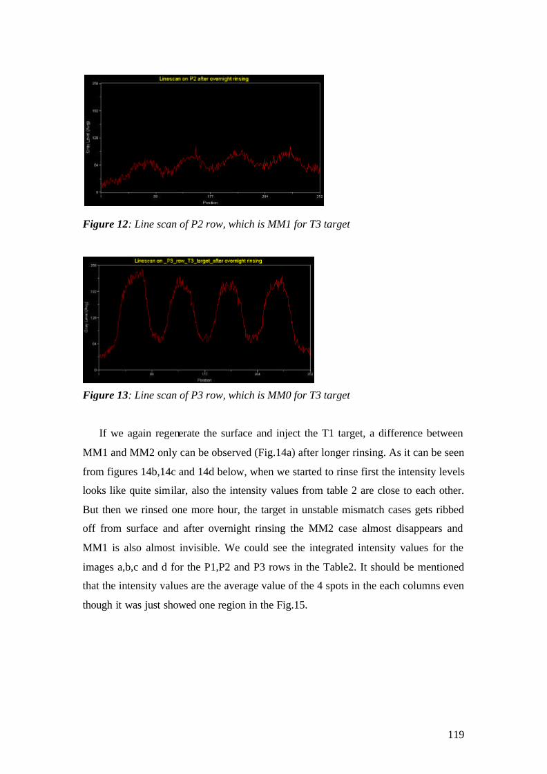
119
Figure 12: Line scan of P2 row, which is MM1 for T3 target
Figure 13: Line scan of P3 row, which is MM0 for T3 target
If we again regenerate the surface and inject the T1 target, a difference between
MM1 and MM2 only can be observed (Fig.14a) after longer rinsing. As it can be seen
from figures 14b,14c and 14d below, when we started to rinse first the intensity levels
looks like quite similar, also the intensity values from table 2 are close to each other.
But then we rinsed one more hour, the target in unstable mismatch cases gets ribbed
off from surface and after overnight rinsing the MM2 case almost disappears and
MM1 is also almost invisible. We could see the integrated intensity values for the
images a,b,c and d for the P1,P2 and P3 rows in the Table2. It should be mentioned
that the intensity values are the average value of the 4 spots in the each columns even
though it was just showed one region in the Fig.15.
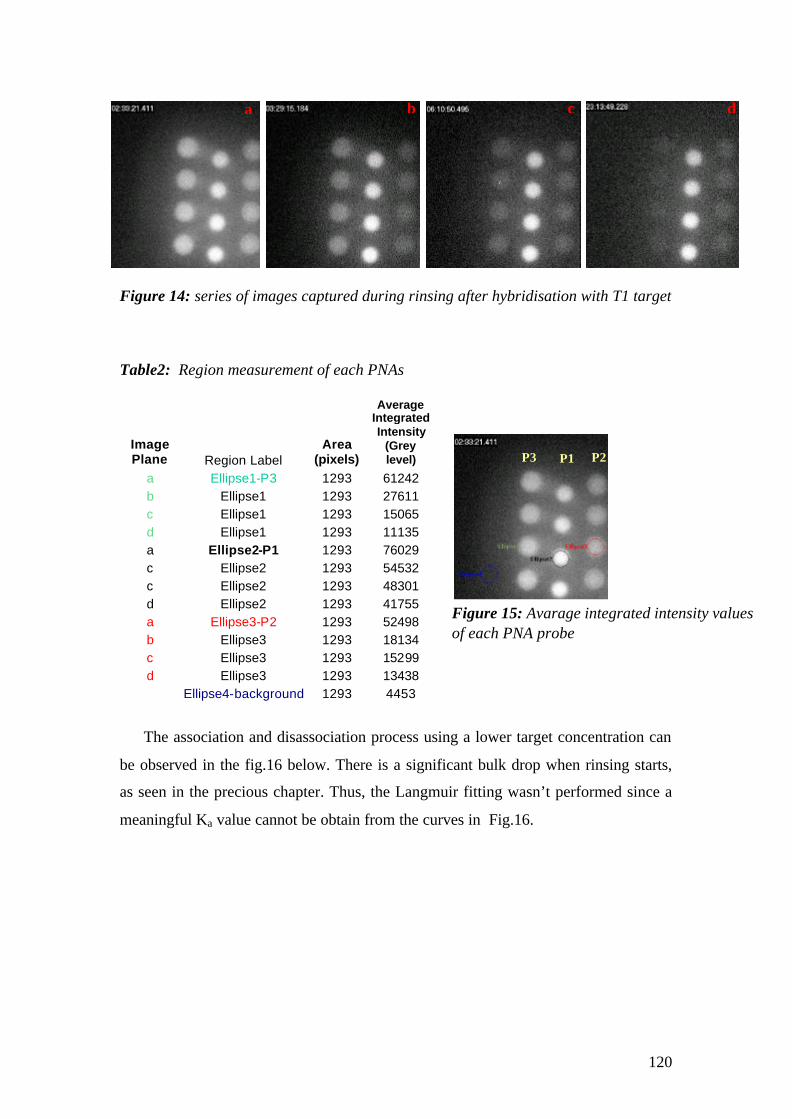
120
Figure 14: series of images captured during rinsing after hybridisation with T1 target
Table2: Region measurement of each PNAs
The association and disassociation process using a lower target concentration can
be observed in the fig.16 below. There is a significant bulk drop when rinsing starts,
as seen in the precious chapter. Thus, the Langmuir fitting wasn’t performed since a
meaningful Ka value cannot be obtain from the curves in Fig.16.
Image Plane Region Label
Area (pixels)
Average Integrated Intensity
(Grey level)
a Ellipse1-P3 1293 61242 b Ellipse1 1293 27611 c Ellipse1 1293 15065 d Ellipse1 1293 11135 a Ellipse2-P1 1293 76029 c Ellipse2 1293 54532 c Ellipse2 1293 48301 d Ellipse2 1293 41755 a Ellipse3-P2 1293 52498 b Ellipse3 1293 18134 c Ellipse3 1293 15299 d Ellipse3 1293 13438 Ellipse4-background 1293 4453
a b c d
P3 P1 P2
Figure 15: Avarage integrated intensity values of each PNA probe

121
0 20000 40000 60000 80000 100000
0
20000
40000
60000
80000
100000
120000in
tegr
ated
inte
nsity
Time (sec)
P1 P2 P3
Figure 16: Langmuir isotherm of P1(MM0),P2(MM1) and P3(MM2) probes after hybridisation with 100nM T1 target.
The homogeneity of the spots is also important for the quantification purposes.
We do statistics about spot-to-spot variation; we can see from the Table 3 that the
spots are quite homogenous although this is not always the usual case. The spot size
strongly dependent on the humidity during the spotting and probe concentration but
most of the probes are commercially supplied or received from the collaborators, it’s
difficult to get samples in very high concentrations as it was also mentioned earlier.
Table 3: Spot-to-spot variation
Beside the differentiation of the MMs, another aim of the project was to
investigate, if GMO can be detected on an array base using SPFM. In the following
chapter this detection will be also performed by using PNA .
Spot Label
Average Intensity
Intensity Standard
Dev
Intensity Signal/Noise
Integrated Intensity
119,016
53,4606
2,22623
293731
122,252
42,834
2,85409
241326
126,925
49,1318
2,58335
276315
125,303
51,7738
2,42019
268649
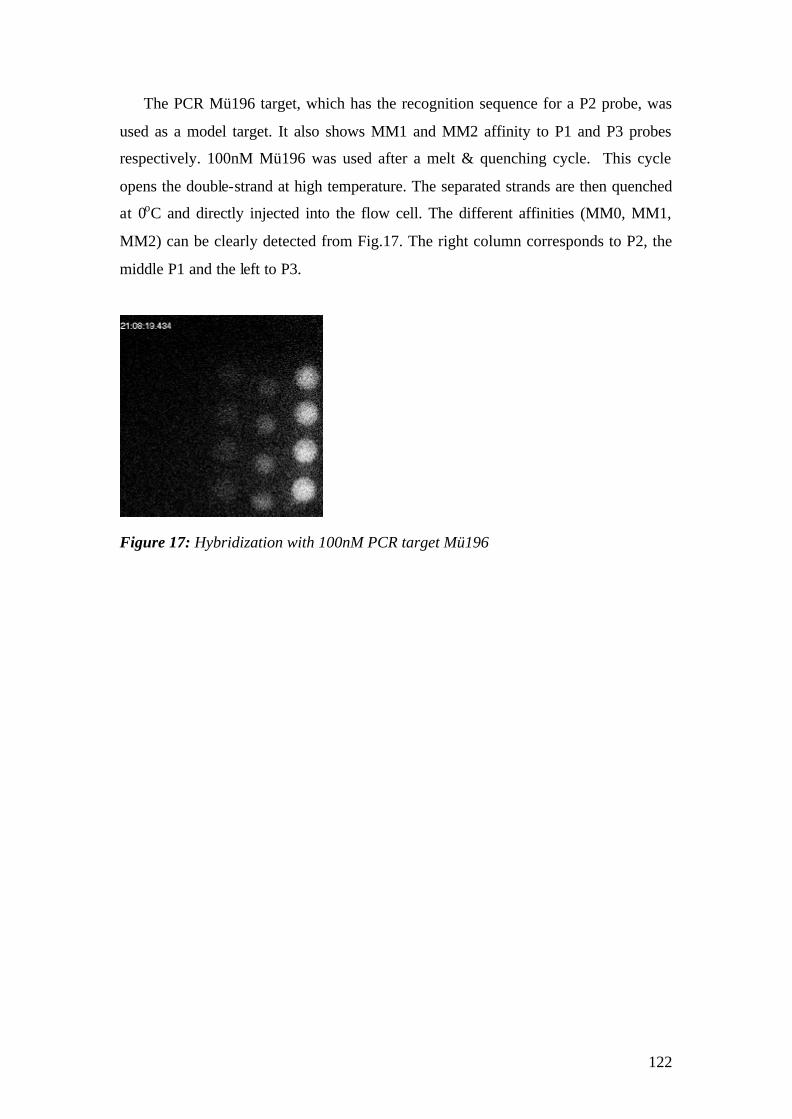
122
The PCR Mü196 target, which has the recognition sequence for a P2 probe, was
used as a model target. It also shows MM1 and MM2 affinity to P1 and P3 probes
respectively. 100nM Mü196 was used after a melt & quenching cycle. This cycle
opens the double-strand at high temperature. The separated strands are then quenched
at 0oC and directly injected into the flow cell. The different affinities (MM0, MM1,
MM2) can be clearly detected from Fig.17. The right column corresponds to P2, the
middle P1 and the left to P3.
Figure 17: Hybridization with 100nM PCR target Mü196

123
We now move from model systems to actual DNAs corresponding to GMO
relevant system.
The following DNA probes were designed according to the GMO sequences. The
array (Fig. 18) of the DNA probes listed in Table 2 was prepared and used for the
GMO detection.
Table 4: DNA probes and target sequences
RR15merMMO (Mismatch 0)
5`-TTT TTT TTT TTT TTT TGC TAG AGT CAG CTT-3`
RR15merMM1 (Mismatch 1)
5`-TTT TTT TTT TTT TTT TGC TAG AGC CAG CTT-3`
SL15merMM0 (Mismatch 0)
5´-TTT TTT TTT TTT TTT GAT CAA GTC GTC GCT-3´
SL15merMM1 (Mismatch 1)
5´-TTT TTT TTT TTT TTT GAT CAA GTT GTC GCT-3´
Target DNA15mer MM1 GMO RR125
Cy5- AAG CTG GCTCTAGCA -3'
DNA name Sequence
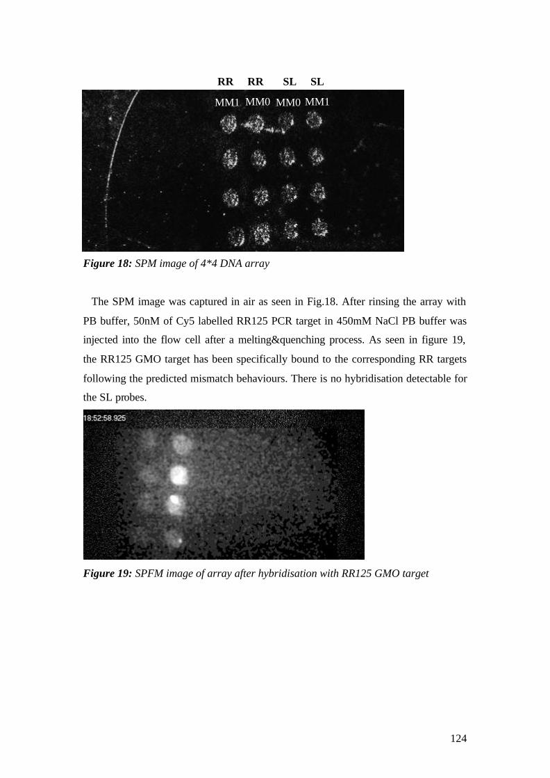
124
Figure 18: SPM image of 4*4 DNA array
The SPM image was captured in air as seen in Fig.18. After rinsing the array with
PB buffer, 50nM of Cy5 labelled RR125 PCR target in 450mM NaCl PB buffer was
injected into the flow cell after a melting&quenching process. As seen in figure 19,
the RR125 GMO target has been specifically bound to the corresponding RR targets
following the predicted mismatch behaviours. There is no hybridisation detectable for
the SL probes.
Figure 19: SPFM image of array after hybridisation with RR125 GMO target
RR RR SL SL
MM1 MM0 MM0 MM1
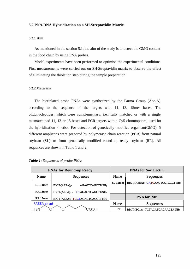
125
5.2 PNA-DNA Hybridization on a SH-Streptavidin Matrix
5.2.1 Aim
As mentioned in the section 5.1, the aim of the study is to detect the GMO content
in the food chain by using PNA probes.
Model experiments have been performed to optimise the experimental conditions.
First measurements were carried out on SH-Streptavidin matrix to observe the effect
of eliminating the thiolation step during the sample preparation.
5.2.2 Materials
The biotinlated probe PNAs were synthesized by the Parma Group (App.A)
according to the sequence of the targets with 11, 13, 15mer bases. The
oligonucleotides, which were complementary, i.e., fully matched or with a single
mismatch had 11, 13 or 15 bases and PCR targets with a Cy5 chromophore, used for
the hybridization kinetics. For detection of genetically modified organism(GMO), 5
different amplicons were prepared by polymerase chain reaction (PCR) from natural
soybean (SL) or from genetically modified round-up ready soybean (RR). All
sequences are shown in Table 1 and 2.
Table 1: Sequences of probe PNAs
BIOT - ( AEEA ) 2 - GATCAAGTCGTCGCT - NH 2 SL 15mer BIOT - ( AEEA ) 2 - AGAGTCAGCTT - NH 2
BIOT - ( AEEA ) 2 - CTAGAGTCAGCTT - NH 2
BIOT - ( AEEA ) 2 - TGCTAGAGTCAGCTT - NH 2
RR 11mer
RR 13mer
RR 15mer
Sequences Sequences Name Name
PNAs for Soy Lectin PNAs for Round - up Ready
BIOT - ( AEEA ) 2 - GATCAAGTCGTCGCT - NH 2 SL 15mer BIOT - ( AEEA ) 2 - AGAGTCAGCTT - NH 2
BIOT - ( AEEA ) 2 - CTAGAGTCAGCTT - NH 2
BIOT - ( AEEA ) 2 - TGCTAGAGTCAGCTT - NH 2
RR 11mer
RR 13mer
RR 15mer
Sequences Sequences Name Name
PNAs for Soy Lectin PNAs for Round - up Ready
Sequences Name
PNA for Mu
BIOT - (EG1) 9 - TGTACATCACAACTA - NH 2 P2 Sequences Name
PNA for Mu
BIOT - (EG1) 9 - TGTACATCACAACTA - NH 2 H2N O O COOH
*AEEA or eg1
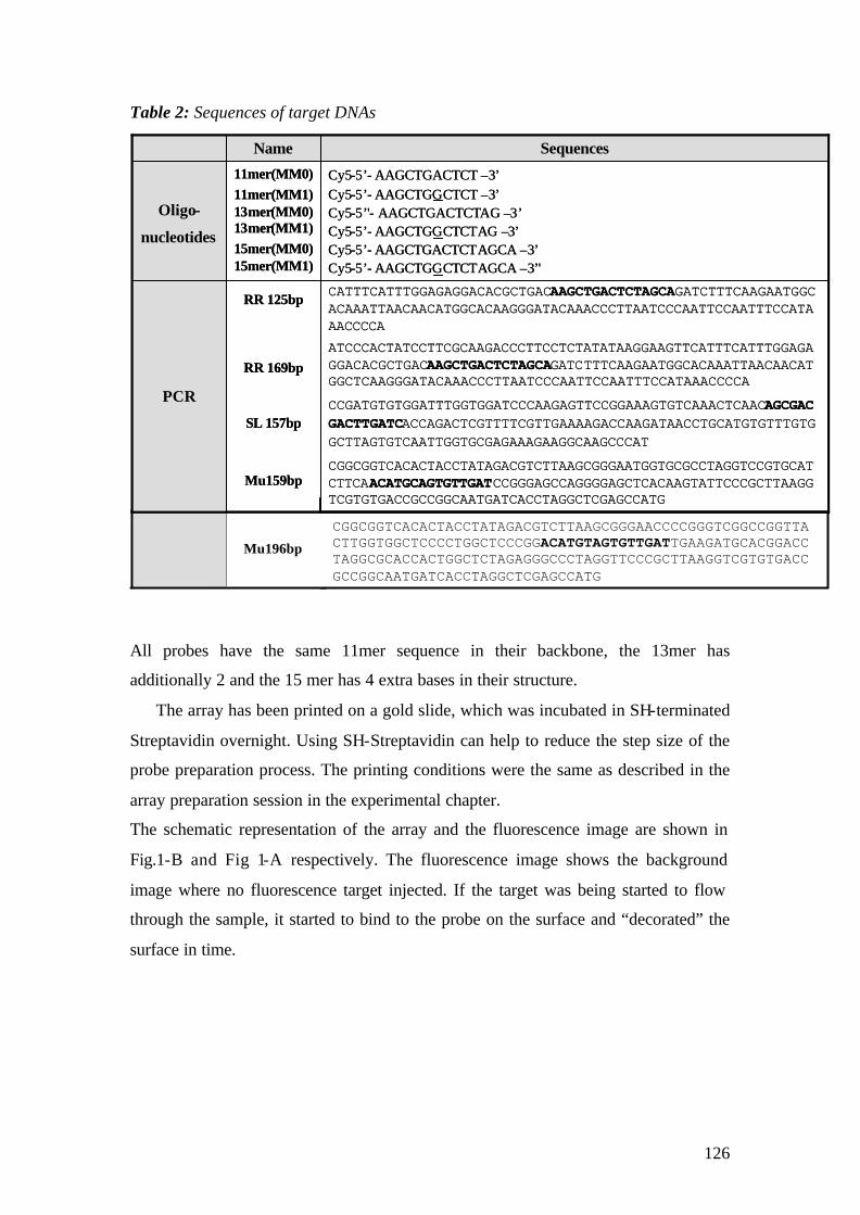
126
Table 2: Sequences of target DNAs
All probes have the same 11mer sequence in their backbone, the 13mer has
additionally 2 and the 15 mer has 4 extra bases in their structure.
The array has been printed on a gold slide, which was incubated in SH-terminated
Streptavidin overnight. Using SH-Streptavidin can help to reduce the step size of the
probe preparation process. The printing conditions were the same as described in the
array preparation session in the experimental chapter.
The schematic representation of the array and the fluorescence image are shown in
Fig.1-B and Fig 1-A respectively. The fluorescence image shows the background
image where no fluorescence target injected. If the target was being started to flow
through the sample, it started to bind to the probe on the surface and “decorated” the
surface in time. A)
CGGCGGTCACACTACCTATAGACGTCTTAAGCGGGAACCCCGGGTCGGCCGGTTACTTGGTGGCTCCCCTGGCTCCCGGACATGTAGTGTTGATTGAAGATGCACGGACCTAGGCGCACCACTGGCTCTAGAGGGCCCTAGGTTCCCGCTTAAGGTCGTGTGACCGCCGGCAATGATCACCTAGGCTCGAGCCATG
Mu196bp
CATTTCATTTGGAGAGGACACGCTGACAAGCTGACTCTAGCAGATCTTTCAAGAATGGCACAAATTAACAACATGGCACAAGGGATACAAACCCTTAATCCCAATTCCAATTTCCATAAACCCCAATCCCACTATCCTTCGCAAGACCCTTCCTCTATATAAGGAAGTTCATTTCATTTGGAGAGGACACGCTGACAAGCTGACTCTAGCAGATCTTTCAAGAATGGCACAAATTAACAACATGGCTCAAGGGATACAAACCCTTAATCCCAATTCCAATTTCCATAAACCCCA
CCGATGTGTGGATTTGGTGGATCCCAAGAGTTCCGGAAAGTGTCAAACTCAACAGCGACGACTTGATCACCAGACTCGTTTTCGTTGAAAAGACCAAGATAACCTGCATGTGTTTGTGGCTTAGTGTCAATTGGTGCGAGAAAGAAGGCAAGCCCAT
CGGCGGTCACACTACCTATAGACGTCTTAAGCGGGAATGGTGCGCCTAGGTCCGTGCATCTTCAACATGCAGTGTTGATCCGGGAGCCAGGGGAGCTCACAAGTATTCCCGCTTAAGGTCGTGTGACCGCCGGCAATGATCACCTAGGCTCGAGCCATG
RR 125bp
RR 169bp
SL 157bp
Mu159bp
PCR
11mer(MM0)11mer(MM1) 13mer(MM0)13mer(MM1)15mer(MM0)15mer(MM1)
Name
Cy5-5’- AAGCTGACTCT –3’Cy5-5’- AAGCTGGCTCT –3’Cy5-5’'- AAGCTGACTCTAG –3’Cy5-5’- AAGCTGGCTCTAG –3’Cy5-5’- AAGCTGACTCTAGCA –3’Cy5-5’- AAGCTGGCTCTAGCA –3’'
Oligo-
nucleotides
Sequences
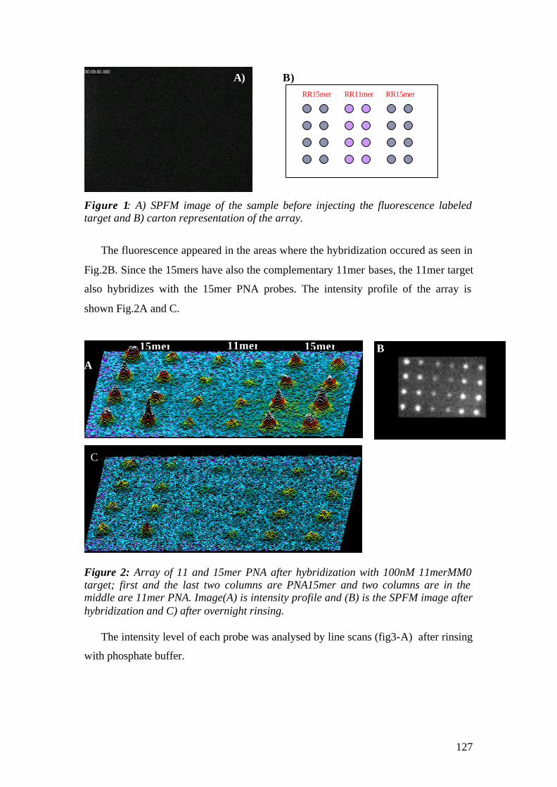
127
Figure 1: A) SPFM image of the sample before injecting the fluorescence labeled target and B) carton representation of the array.
The fluorescence appeared in the areas where the hybridization occured as seen in
Fig.2B. Since the 15mers have also the complementary 11mer bases, the 11mer target
also hybridizes with the 15mer PNA probes. The intensity profile of the array is
shown Fig.2A and C.
Figure 2: Array of 11 and 15mer PNA after hybridization with 100nM 11merMM0 target; first and the last two columns are PNA15mer and two columns are in the middle are 11mer PNA. Image(A) is intensity profile and (B) is the SPFM image after hybridization and C) after overnight rinsing. The intensity level of each probe was analysed by line scans (fig3-A) after rinsing
with phosphate buffer.
A
C
15mer 11mer 15mer B
RR15mer RR11mer RR15mer
B) A)
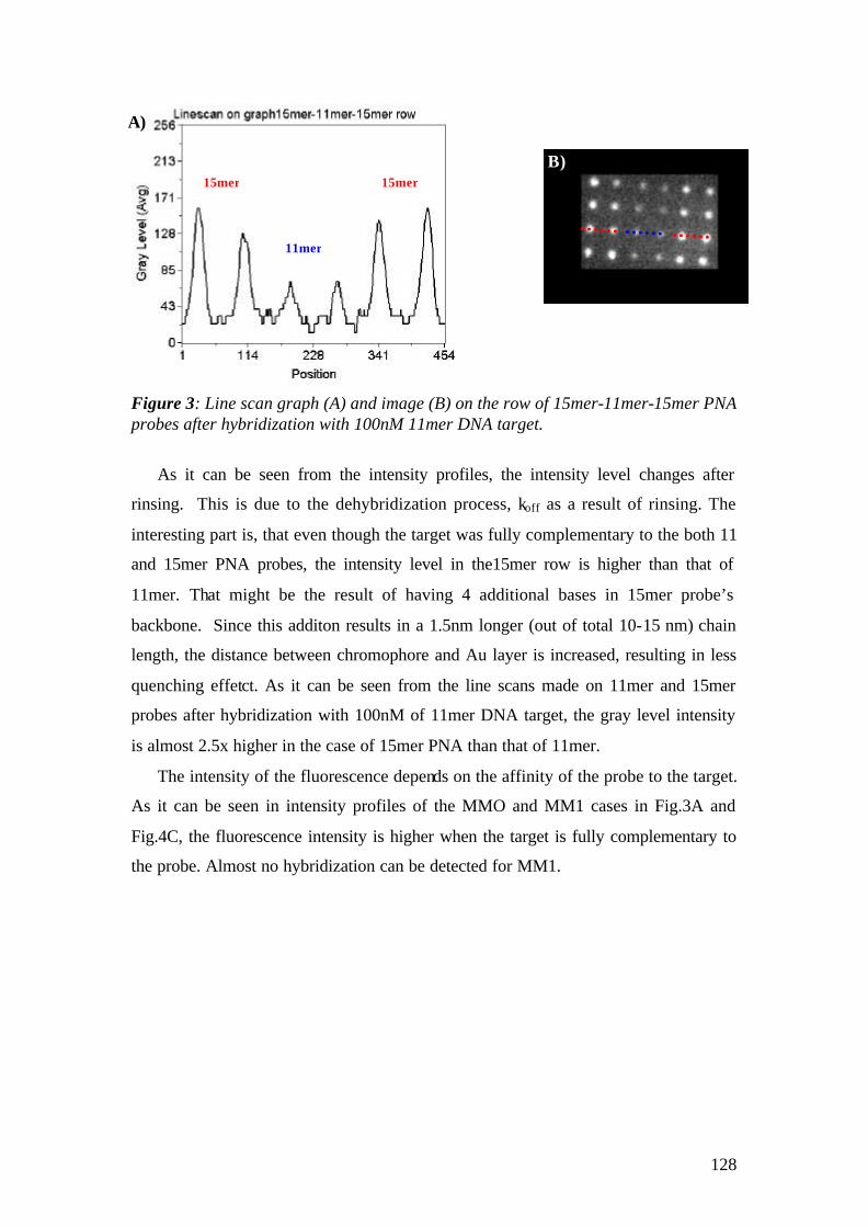
128
Figure 3: Line scan graph (A) and image (B) on the row of 15mer-11mer-15mer PNA probes after hybridization with 100nM 11mer DNA target.
As it can be seen from the intensity profiles, the intensity level changes after
rinsing. This is due to the dehybridization process, koff as a result of rinsing. The
interesting part is, that even though the target was fully complementary to the both 11
and 15mer PNA probes, the intensity level in the15mer row is higher than that of
11mer. That might be the result of having 4 additional bases in 15mer probe’s
backbone. Since this additon results in a 1.5nm longer (out of total 10-15 nm) chain
length, the distance between chromophore and Au layer is increased, resulting in less
quenching effetct. As it can be seen from the line scans made on 11mer and 15mer
probes after hybridization with 100nM of 11mer DNA target, the gray level intensity
is almost 2.5x higher in the case of 15mer PNA than that of 11mer.
The intensity of the fluorescence depends on the affinity of the probe to the target.
As it can be seen in intensity profiles of the MMO and MM1 cases in Fig.3A and
Fig.4C, the fluorescence intensity is higher when the target is fully complementary to
the probe. Almost no hybridization can be detected for MM1.
15mer
11mer
15mer B)
A)
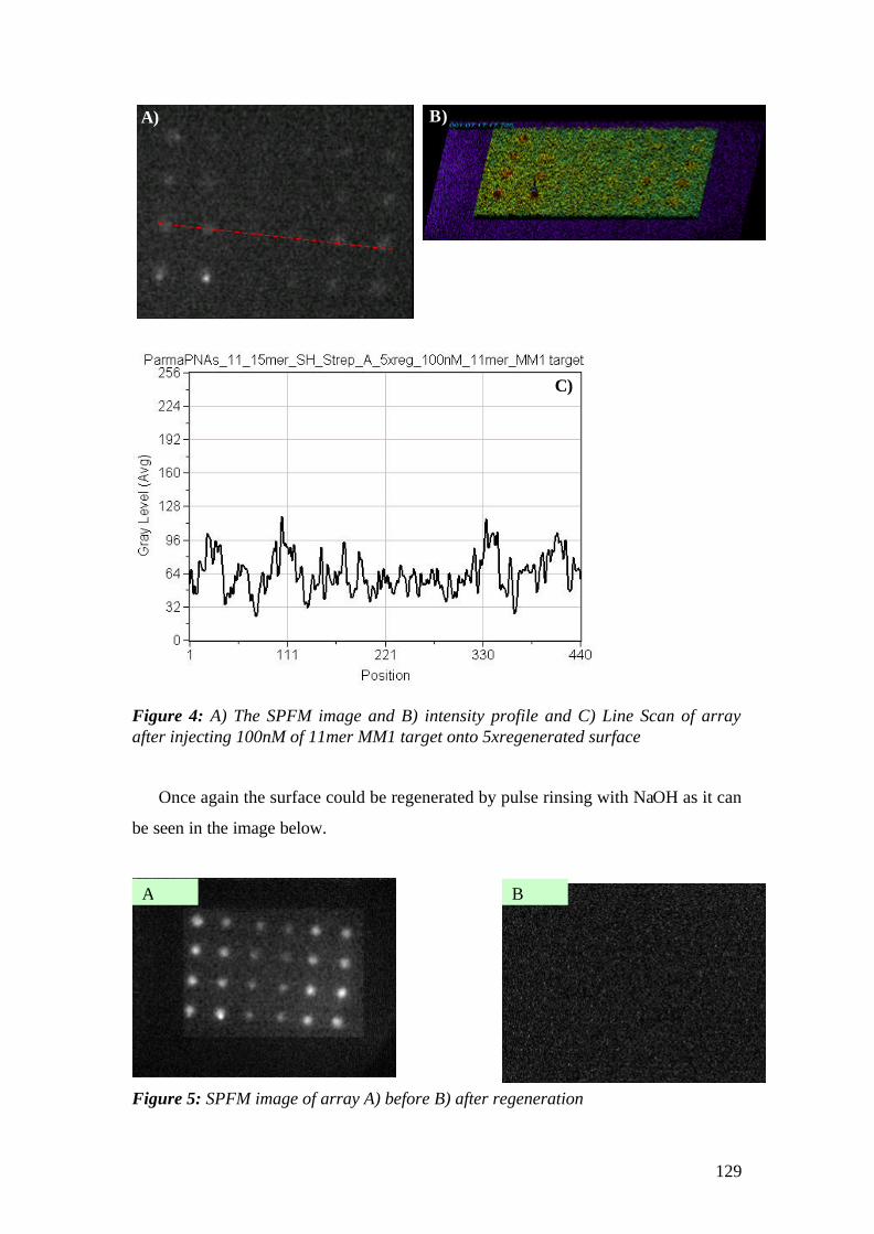
129
Figure 4: A) The SPFM image and B) intensity profile and C) Line Scan of array after injecting 100nM of 11mer MM1 target onto 5xregenerated surface Once again the surface could be regenerated by pulse rinsing with NaOH as it can
be seen in the image below.
Figure 5: SPFM image of array A) before B) after regeneration
B A
C)
A) B)

130
Two different SPFS measurement were performed in order to investigate the
importance of the SAM step for the fluorescence measurement in further experiments
design. For that purpose a RR11mer PNA probe and a RR15mer MM0 DNA target
were used. Both measurements were performed in 10mM phosphate buffer under the
same experimental conditions. The first measurement in Fig.6-A shows the
measurement with SH-Streptavidin and Fig.6-B with SAM/Streptavidin matrix by
using 100nM and 50nM target respectively. When we compare the two
measurements, we can easily see that the fluorescence signal differs in the SH-
streptavidin case in the rinsing step. Since the rinsing step is independent from the
target concentration, the only reason for this result might be quenching of the
fluorescence. Once the target solution is replaced with the pure buffer and the
dissociation of the targets from their probes leads to a decrease of the measured
fluorescence as a function of time by coupling their energy back to the metal layer.
Even though a MM0 target was used in both cases, the fluorescence intensity in the
SAM matrix case decreases slowly while the SH-Streptavidin case shows a sharper
decay. This effect cannot be observed in the association phase because relatively high
target concentration were used, there are always an exchange between bleached
chromophores and fresh ones from solution.
Figure 6: SPFS measurement of DNA RR15mer target hybridisation with PNA11mer probe immobilized onto A) SH-Streptavidin, B)biotinylated thiol/OH-thiol mixure/streptavidin matrixes
0 100 200 300 400 500
0
1x10⁵
2x10⁵
3x10⁵
4x10⁵
Flu
ores
cenc
e/cp
s
Time/min.
MM0
MM1
Rinsing
Rinsing
0 100 200 300 400 500
0
1x10⁵
2x10⁵
3x10⁵
4x10⁵
Flu
ores
cenc
e/cp
s
Time/min.
MM0
MM1
Rinsing
Rinsing
0 100 200 300 400 500
0,0
2,0x10⁴
4,0x10⁴
6,0x10⁴
8,0x10⁴
1,0x10⁵
Flu
ores
cenc
e (c
ps)
time (min)
PNARR11mer/100nM DNA15mer target
Rinsing
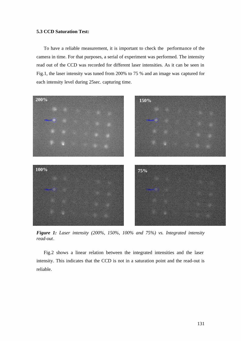
131
5.3 CCD Saturation Test:
To have a reliable measurement, it is important to check the performance of the
camera in time. For that purposes, a serial of experiment was performed. The intensity
read out of the CCD was recorded for different laser intensities. As it can be seen in
Fig.1, the laser intensity was tuned from 200% to 75 % and an image was captured for
each intensity level during 25sec. capturing time.
Figure 1: Laser intensity (200%, 150%, 100% and 75%) vs. Integrated intensity read-out.
Fig.2 shows a linear relation between the integrated intensities and the laser
intensity. This indicates that the CCD is not in a saturation point and the read-out is
reliable.
200% 150%
100% 75%
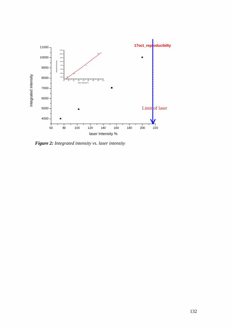
132
Figure 2: Integrated intensity vs. laser intensity
60 80 100 120 140 160 180 200 220
4000
5000
6000
7000
8000
9000
10000
11000
inte
grat
ed in
tens
ity
laser Intensity %
17oct_reproducibilty
6 0 80 100 120 140 160 180 200 220
4000
5000
6000
7000
8000
9000
10000
11000
inte
grat
ed in
tens
ity
laser Intensity %
Limit of laser

133
5.4 PNA-DNA Hybridization on a Biotin thiol / Streptavidin Matrix
5.4.1 Array A:
The following experiments were done as a model system for the combination of
mismatches and specific binding on a same chip. For that purposes, 11 and 15mer
PNA probes, that have mentioned in section 4.3.1 and the probes PNA P1, P2 and P3
(section 4.3.2), that have mismatches in their sequences to the same target have been
used.
Table 1: PNA probes and the complementary targets
The spotting was done by using an ink-jet spotter thiol/biotin-streptavidin
substrate. The humidity of the printing chamber was kept at 70% during the spotting
process. After allowing the probe to react with the streptavidin coated surface for
about 2 hrs, the sample was placed into a sample holder. Fig.1 shows the SPM image
of the array in air.
PNAs for Roundup Ready (RR probes)
11mer: Biotin-AEEA-AEEA- AGAGTCAGCTT -NH2 13mer: Biotin-AEEA-AEEA- CT AGAGTCAGCTT -NH2 15mer: Biotin-AEEA-AEEA- TG CT AGAGTCAGCTT -NH2
DNAs (target)
11mer: Cy5-5'- AAGCTGACTCT -3' 13mer: Cy5-5'- AAGCTGACTCTAG -3' 15mer: Cy5-5'- AAGCTGACTCTAGCA -3'
P1 probe 30 5´-Biotin -T15 TGT ACG TCA CAA CTA -3´ P2 probe 30 5´-Biotin -T15 TGT ACA TCA CAA CTA -3´ P3 probe 30 5´-Biotin -T15 TGT ACG TGA CAA CTA -3´ T1 target 15 5´- Cy5 -TAG TTG TGA CGT ACA -3´ T2 target 15 5´- Cy5 -TAG TTG TGA TGT ACA -3´ T3 target 15 5´- Cy5 -TAG TTG TCA CGT ACA -3´
PPNNAA
DDNNAA ttaarrggee ttss
H2N O O COOH*AEEA:
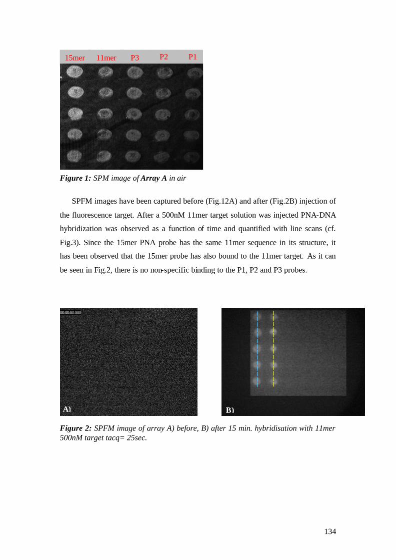
134
Figure 1: SPM image of Array A in air
SPFM images have been captured before (Fig.12A) and after (Fig.2B) injection of
the fluorescence target. After a 500nM 11mer target solution was injected PNA-DNA
hybridization was observed as a function of time and quantified with line scans (cf.
Fig.3). Since the 15mer PNA probe has the same 11mer sequence in its structure, it
has been observed that the 15mer probe has also bound to the 11mer target. As it can
be seen in Fig.2, there is no non-specific binding to the P1, P2 and P3 probes.
Figure 2: SPFM image of array A) before, B) after 15 min. hybridisation with 11mer 500nM target tacq= 25sec.
15mer P3 P2 P1 11mer
A) B)
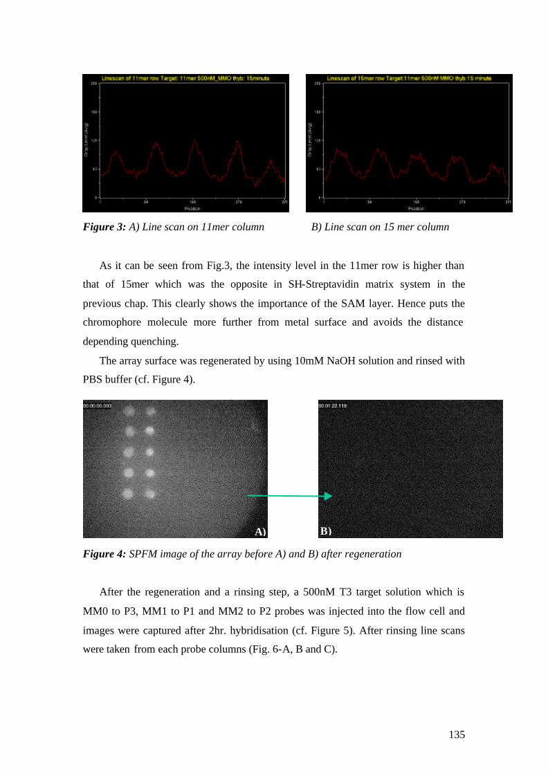
135
Figure 3: A) Line scan on 11mer column B) Line scan on 15 mer column
As it can be seen from Fig.3, the intensity level in the 11mer row is higher than
that of 15mer which was the opposite in SH-Streptavidin matrix system in the
previous chap. This clearly shows the importance of the SAM layer. Hence puts the
chromophore molecule more further from metal surface and avoids the distance
depending quenching.
The array surface was regenerated by using 10mM NaOH solution and rinsed with
PBS buffer (cf. Figure 4).
Figure 4: SPFM image of the array before A) and B) after regeneration
After the regeneration and a rinsing step, a 500nM T3 target solution which is
MM0 to P3, MM1 to P1 and MM2 to P2 probes was injected into the flow cell and
images were captured after 2hr. hybridisation (cf. Figure 5). After rinsing line scans
were taken from each probe columns (Fig. 6-A, B and C).
A) B)
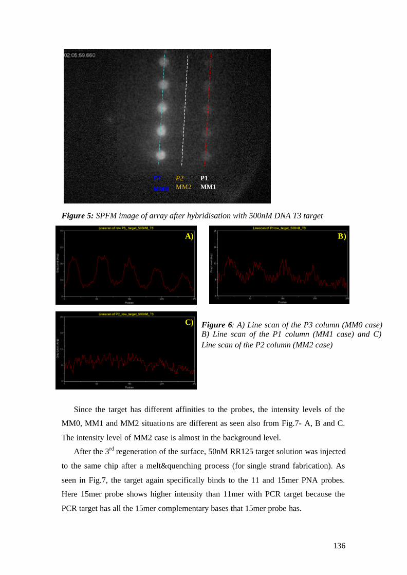
136
Figure 5: SPFM image of array after hybridisation with 500nM DNA T3 target
Since the target has different affinities to the probes, the intensity levels of the
MM0, MM1 and MM2 situations are different as seen also from Fig.7- A, B and C.
The intensity level of MM2 case is almost in the background level.
After the 3rd regeneration of the surface, 50nM RR125 target solution was injected
to the same chip after a melt&quenching process (for single strand fabrication). As
seen in Fig.7, the target again specifically binds to the 11 and 15mer PNA probes.
Here 15mer probe shows higher intensity than 11mer with PCR target because the
PCR target has all the 15mer complementary bases that 15mer probe has.
P3
MM0 P2 MM2
P1 MM1
Figure 6: A) Line scan of the P3 column (MM0 case) B) Line scan of the P1 column (MM1 case) and C) Line scan of the P2 column (MM2 case)
A) B)
C)
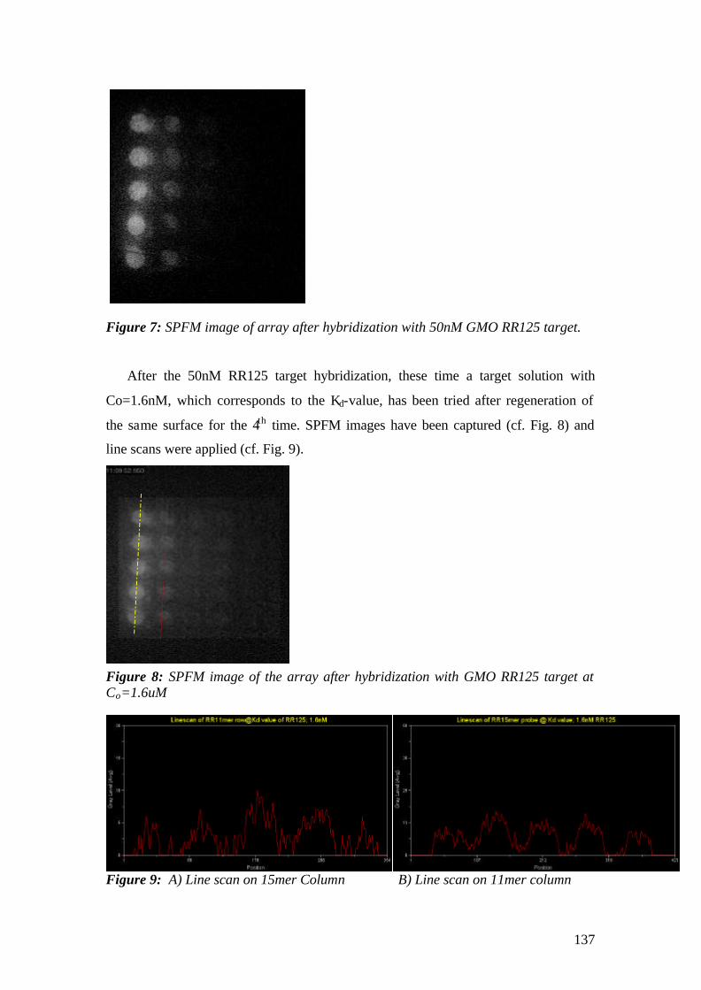
137
Figure 7: SPFM image of array after hybridization with 50nM GMO RR125 target.
After the 50nM RR125 target hybridization, these time a target solution with
Co=1.6nM, which corresponds to the Kd-value, has been tried after regeneration of
the same surface for the 4th time. SPFM images have been captured (cf. Fig. 8) and
line scans were applied (cf. Fig. 9).
Figure 8: SPFM image of the array after hybridization with GMO RR125 target at Co=1.6uM
Figure 9: A) Line scan on 15mer Column B) Line scan on 11mer column
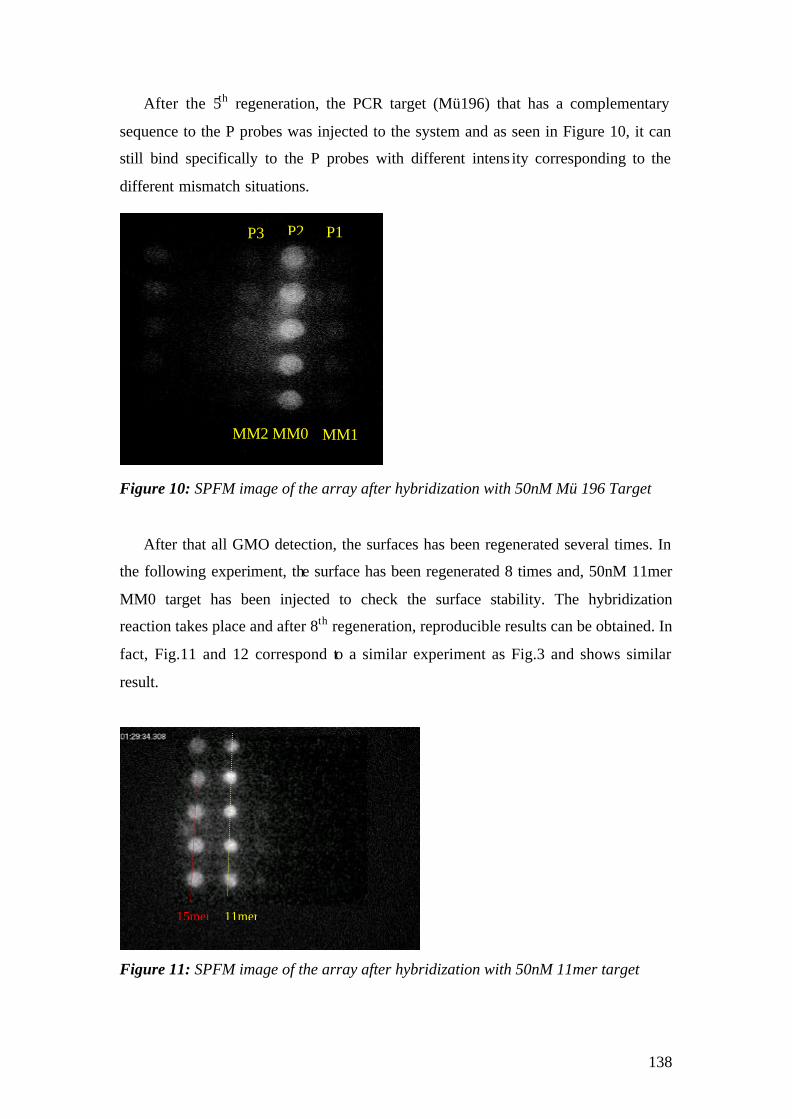
138
After the 5th regeneration, the PCR target (Mü196) that has a complementary
sequence to the P probes was injected to the system and as seen in Figure 10, it can
still bind specifically to the P probes with different intens ity corresponding to the
different mismatch situations.
Figure 10: SPFM image of the array after hybridization with 50nM Mü 196 Target
After that all GMO detection, the surfaces has been regenerated several times. In
the following experiment, the surface has been regenerated 8 times and, 50nM 11mer
MM0 target has been injected to check the surface stability. The hybridization
reaction takes place and after 8th regeneration, reproducible results can be obtained. In
fact, Fig.11 and 12 correspond to a similar experiment as Fig.3 and shows similar
result.
Figure 11: SPFM image of the array after hybridization with 50nM 11mer target
P3 P2 P1
MM2 MM0 MM1
15mer 11mer

139
Figure 12: Line Scans after hybridization with 50nM 11mer MM0 target on A) 15mer row B) 11mer row.
5.4.2 Array B:
All Parma PNAs have been spotted using a Pin-tool spotter under the same
conditions and having the same surface chemistry that has been described in the Array
A. This array represents the final goal of the project, which is determination of GMO
ingredient (RR target) from natural component (SL targets) in the food. The SPM
image of the array is shown in Fig.1.
Figure 1: SPM image of Array B in air (All Parma PNAs at 1µM probe concentration)
SL 15
SL 13
SL 11
Mis RR 15
RR 15
RR 13
RR 11
MisRR 13
Mis RR 11
A) B)
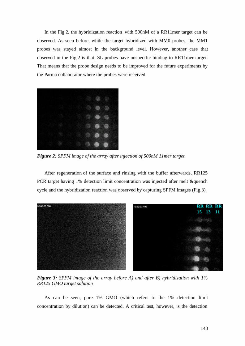
140
In the Fig.2, the hybridization reaction with 500nM of a RR11mer target can be
observed. As seen before, while the target hybridized with MM0 probes, the MM1
probes was stayed almost in the background level. However, another case that
observed in the Fig.2 is that, SL probes have unspecific binding to RR11mer target.
That means that the probe design needs to be improved for the future experiments by
the Parma collaborator where the probes were received.
Figure 2: SPFM image of the array after injection of 500nM 11mer target
After regeneration of the surface and rinsing with the buffer afterwards, RR125
PCR target having 1% detection limit concentration was injected after melt &quench
cycle and the hybridization reaction was observed by capturing SPFM images (Fig.3).
Figure 3: SPFM image of the array before A) and after B) hybridization with 1% RR125 GMO target solution
As can be seen, pure 1% GMO (which refers to the 1% detection limit
concentration by dilution) can be detected. A critical test, however, is the detection
RR 15
RR 13
RR 11
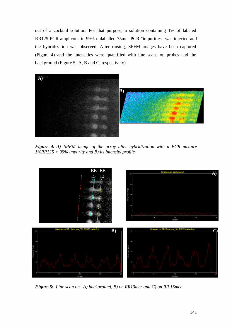
141
out of a cocktail solution. For that purpose, a solution containing 1% of labeled
RR125 PCR amplicons in 99% unlabelled 75mer PCR "impurities" was injected and
the hybridization was observed. After rinsing, SPFM images have been captured
(Figure 4) and the intensities were quantified with line scans on probes and the
background (Figure 5- A, B and C, respectively)
Figure 4: A) SPFM image of the array after hybridization with a PCR mixture 1%RR125 + 99% impurity and B) its intensity profile
Figure 5: Line scan on A) background, B) on RR13mer and C) on RR 15mer
RR 15
RR 13
A)
B) C)
A)
B)
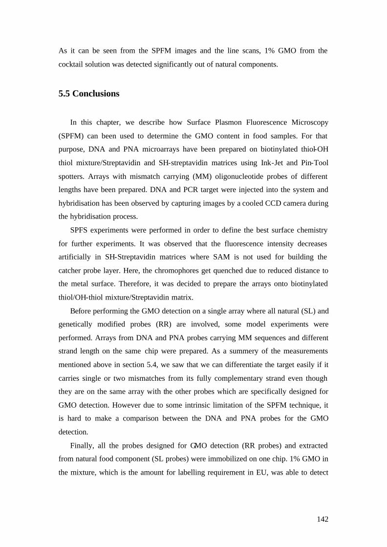
142
As it can be seen from the SPFM images and the line scans, 1% GMO from the
cocktail solution was detected significantly out of natural components.
5.5 Conclusions
In this chapter, we describe how Surface Plasmon Fluorescence Microscopy
(SPFM) can been used to determine the GMO content in food samples. For that
purpose, DNA and PNA microarrays have been prepared on biotinylated thiol-OH
thiol mixture/Streptavidin and SH-streptavidin matrices using Ink-Jet and Pin-Tool
spotters. Arrays with mismatch carrying (MM) oligonucleotide probes of different
lengths have been prepared. DNA and PCR target were injected into the system and
hybridisation has been observed by capturing images by a cooled CCD camera during
the hybridisation process.
SPFS experiments were performed in order to define the best surface chemistry
for further experiments. It was observed that the fluorescence intensity decreases
artificially in SH-Streptavidin matrices where SAM is not used for building the
catcher probe layer. Here, the chromophores get quenched due to reduced distance to
the metal surface. Therefore, it was decided to prepare the arrays onto biotinylated
thiol/OH-thiol mixture/Streptavidin matrix.
Before performing the GMO detection on a single array where all natural (SL) and
genetically modified probes (RR) are involved, some model experiments were
performed. Arrays from DNA and PNA probes carrying MM sequences and different
strand length on the same chip were prepared. As a summery of the measurements
mentioned above in section 5.4, we saw that we can differentiate the target easily if it
carries single or two mismatches from its fully complementary strand even though
they are on the same array with the other probes which are specifically designed for
GMO detection. However due to some intrinsic limitation of the SPFM technique, it
is hard to make a comparison between the DNA and PNA probes for the GMO
detection.
Finally, all the probes designed for GMO detection (RR probes) and extracted
from natural food component (SL probes) were immobilized on one chip. 1% GMO in
the mixture, which is the amount for labelling requirement in EU, was able to detect

143
specifically from the natural food component (SL) by using SPFM technique on an
array platform.
Using SPFM, we could easily detect 1% GMO out of a mixture. This value
corresponds to the amount, which requires labelling according to the EU laws.
Therefore we could show that the SPFM technique, presented in this work, is well
suitable for the detection of genetically modified genes in food chain. However, for
future SPFM experiments, it is important to consider the probe design.

144
List of Figures Chpt1-2 Figure 1: Schematic representation of the double helix (left) showing the minor and the major groove, a DNA single-strand illustrating the way the sugar units are linked via the H-bonding between specific Watson-Crick base pairs (right) and phosphodiester bridges (middle)…………………………………………………………. ..8 Figure 2: The structure of PNA and hybridization scheme with DNA strand………..10 Figure3: Target strand amplification by PCR (http://allserv.rug.ac.be/~avierstr/pdf/PCR.pdf)………………………………………... 14 Figure 4: Ink-jet spotter……………………………………………………………………..19 Figure 5: a) Pin Tool spotter and b)Tip position from surface)………………………..20 Figure 6: a) Solid pin, b) Split pin (www.pointech.com)………………………………..20 Figure 7: Effect of spotting solution on spot quality, right image is without spotting solution and the left one is with spotting solution (www.telechem.com)………………21 Figure 8: Jablonski energy level diagram………………………………………………...22 Figure 9: Schematic description of Langmuir adsorption. As it can be seen from the graph, the surface coverage is dependent on adsorption and desorption rate constants, kon and k off respectively………………………………………………………….26 Figure 10: The basic configuration for evanescent optics………………………………29 Figure 11: Schematic representation of reflected and transmitted P-polarized light at the interface between two optically different media …………………………………….30 Figure 12: Dispersion relation for A) free photons in a dielectric, B) free photons propagating in a coupling prism, SP1) surface plasmons at a metal/dielectric interface and SP2) surface plasmons after adsorption of an additional dielectric layer [Liebermann, 1999]. …………………………………………………………………………33 Figure 13 a) Reflection geometry for photons with a momentum kph at a metal/dielectric interface. The angle of incidence θ determines the absolute value of the momentum in z-direction, kph, x, that is relevant for surface plasmon excitation. b) Kretschmann configuration for momentum matching via prism coupling…………… 34 Figure 14: As it was described in the text above, resonant coupling is observed as a very pronounced drop in angular scan of the reflected light intensity at θR. θc is the critical angle for Total Internal Reflection (TIR)………………………………………..35

145
Figure 15: a) Scan curves of Biotin-Streptavidin binding onto biotinylated/OH-terminated thiol modified Au surface. The resonance angle shift is around 0.5 degree since streptavidin is a big bulk molecule which has molecular weight around 60K. b) kinetic curve of streptavidin binding onto same surface. The binding was observed at fixed resonance angle by following the reflective index change in time. …………………………………………………………………………………………………..36 Figure 16: Schematic drawing of a fluorophore positioned close to a metal/dielectric interface. Different fluorescence decay channels take place at different fluorophore/metal separation distances…………………………………………………...38 Figure 17: Schematic representation of SPM & SPFM set-up (from Rothenhäusler et al., 488, 1988, Nature)………………………………………………………………...……..40 Figure 18: Schematic representation of SPM and SPFM techniques with a 3D spatial filter configuration…………………………………………………………………...………41 Chpt.3 Figure 1: Schematic sketch of a surface plasmon spectrometer (SPR) set-up including various extensions. The whole set-up including the motors of the goniometer is remote controlled by a personal computer using the software WASPLAS………………………………………………………….………………………....45 Figure 2: Actual picture of the SPR set-up with different modifications: A) CCD Camera, B) 3D beam expander………………….………………………………………….46 Figure 3: experimental set-up of SPM (taken from dissertation of Thomas Neumann ……………………………………….………………………………………………..……….47 Figure 4: Chemical structure of a) 1-mercapto-undecanole and b) 11-mercapto-(8-biotinamido-4, 7, dioxaoctyl-)-undecanoylamide, (c) Schematic of the self-assembly process. The anchor group, in this case S-H, has a strong chemical affinity to the gold surface. A covalent Au-S-bond is spontaneously formed by the mere exposure of the thiol solution to the gold surface. In the course of the reaction, all available binding sites on the gold surface are occupied by thiol molecules. The alkyl-chains adopt a parallel orientation with a uniform tilt angle of 30° relative to the surface normal. Such a highly ordered surface architecture meets perfectly the steric requirements for streptavidin binding (right cartoon)………………………………………………………..49 Figure 5: Schematic representation of a mixed monolayer of biotin- and EG (spacer)- thiol (with a molar ratio of 1:9 in the preparation solution) covered with streptavidin, probe and target..…………………………………………………………….………………50 Figure 6: Molecular structure of a single streptavidin tetramer. Four biotin molecules (chemical structure on the right side) are depicted using a ball and stick model………………………………………………………………………………………...51 Figure 7: SPR detection of streptavidin binding. a) resonance angle shift after binding and b) kinetic observation of binding reaction in time………………………..52

146
Figure 8: Construction of the measurement chamber (left) and top view of the flow cell including a schematic of the circulation loop (right)……………………………….53 Figure 9:Angular Scan measurement after probe immobilization……………….……55 Figure 10: A typical SPR scan curve with the fluorescence (SPFS)…………………..56 Figure 11: Single kinetic measurement with fluorescence. 1) Injection of target solution; 2) hybridisation, association phase; 3) saturation of fluorescence signal; 4) start of rinsing; 5) disassociation phase with continued rinsing……………………….57 Figure 12: Chemical structure of Cy5 chromophore, which has its maximum absorbance at λ=649nm and emission at λ=670nm…………………………………….58 Figure 13: a) A typical titration experiment with a concentration range from pM to nM and b) obtaining the binding constant from Langmuir Isotherm fitting……..…...60 Figure 14: Monitoring of the fluorescence vs. time during the regeneration process with 10mM NaOH…………………………………………………………………………….61 Chpt4 Figure 1: Decay channels for fluorescence emitted near a metallic surface A) non-radiative energy transfer, B) coupling of irradiated fluorescence light to SP modes, C) free emission of fluorescence………………………………………………………………..65 Figure 2: Structural formula of 2,6-diaminopurine represented as “D” (C11H14N8O2). …………………………………………………………………………………66 Figure 3: A) Mimic of the neutral thymine nucleobase, 7-chloro-1,8-naphthyridine-2(1H)-one; The Watson-Crick base pair interaction B) between natural Adenin-Thymine, C) Adenine-Modified Thymine bases …………………………………………..67 . Figure 4: Unspecific binding measurement between Lysine and dye………………....69 Figure 5: Single kinetic measurement of PNA2361 with 100nM target concentration in 10 mM ……………………………………………………………………………………...70 Figure 6: A) Single kinetic measurement of PNA2364 and B) its Langmuir fit with the flow rate 2.5ml/min. C) same kinetic measurement with a faster flow rate, 3.6ml/min and using 10nM target concentration and zoomed-in plot of association (small graph)……………………………………………………… ………………………………...71 Figure 7: A) Single kinetic measurement of PNA2367after twice regeneration of the surface and B) Langmuir fitting of kinetic curve…………………………………………72 Figure 8: A) Single kinetic measurement of PNA2370 and B) MM1 case with 100nM target……………………………………………………………………………………………73

147
Figure 9: Single kinetic measurement of PNA2370 with 500pM target concentration in PBS …………………………………………………………………………………………74
Figure 10: Single kinetic measurement of A) PNA2376 and B)PNA2379 with 100nM target …………………………………………………………………………………………..74 Figure 11: Plot of Ka from single kinetic measurement vs. ∆Tm…………………….76 Figure 12: Titration curve of PNA2361 A) MM0 titration experiment B) conventional representation and C) linearized isotherm plots relating target concentrations with respective saturation intensity and b) and c) focused plots of B) and C) respectively……………………………………………………………………………….78-79 Figure 13: Angular scan with fluorescence after saturation of each target concentration in the titration measurement …………………………………………….79 Figure 14: Langmuir isotherm (A) and linerized plot (B) of PNA2361 derived from angular scan with fluorescence…………………………………………………………….80 Figure 15: A) Angular Scan with the fluorescence after each concentration saturation in titration measurement B) Langmuir isotherm C) Linearized curve of PNA2379 derived from angular scan with fluorescence……………………………………………..81 Figure 16: A) titration measurement of PNA2373 and B) Lanmuir fitting for association phase (kon) of plot A…………………………………………………………...83 Figure 17 : Titration measurement of PNA2370 and summary of the kon, koff values from the fitting of plot A and calculated affinity constant from kon/koff………………..84 Figure 18: Comparison of Ka values obtained from single kinetic, saturation and angular scan measurements for the all PNAs……………………………………………..85 Figure 19: Single kinetic measurement with 5 different concentration………………87 Figure 20. Langmuir fitting for dissociation phase of each concentration ………….87 Figure 21. Langmuir fitting for the association phase of A)1nM, B)10nM, C)50, and D)100nM target concentration……………………………………………………………...88 Figure 22. Linear fit of ka vs. concentration plot………………………………………..89 Figure 23: Comparison of association constant, kon, obtained from Single Kinetic measurement and Global Analysis…………………………………………………………90 Figure 24: Comparison of the affinity constants, Ka, obtained from Single Kinetic measurement and from Global Analysis…………………………………………………...91 Figure 25: Ka from Global Analysis vs. ∆Tm……………………………………………..92

148
Figure 26: Plotting of Ka values obtained from Single kinetic, both Saturation and angular scan from titration measurements and Global Analysis measurement vs. ∆Tm
…………………………………………………………………………………………………………………………………..…………………92 Chp4.2 Figure 1: SPM image of Array 2A. CC refers coupling control @ different resonance angle…………………………………………………………………………………………….96 Figure 2: A) Background image, B) SPFM image before any target injected……… 96 Figure 3: SPFM image of the array after hybridizing with 50nM target(A), false color representation(B) and intensity profile(C) of the same image…………………………97
Figure 4: Line scan on A) C5, B) B5 and C) A5 row…………………………………….97 Figure 5: Regionmesurement of the spots on array after rinsing………………………98 Figure 6: A) SPM image of array, A) in air and B) cartoon drawing of the array ….98 Figure 7: A) Line scan image and B) lines scan plot of array after hybridized with 50nM target and rinsed with buffer C) image and region measurement values after overnight rinsing………………………………………………………………………….98-99 Figure 8: Integrated intensity vs. time plotted for each PNA…………………………..99 Figure 9: Zoomed-in plot of Fig.8, Integrated intensity vs. time plotted for each PNA……………………………………………………………………………………………100 Figure 10: Langmuir Fit for C3 column…………………………………………………101 Figure 11: SPM image of array 1A, A) against air and B) cartoon drawing of the array………………………………………………………………………………………….101 Figure 12: SPFM image of array 1 A) after appr.2 hrs rinsing and B) its line scan, C) after overnight rinsing and D) its linescan………………………………………………102 Figure 13: The averaged region measurements of the spots in each row and values summarized in the table…………………………………………………………………….102 Figure 14: Regeneration of array A)before rinsing, B) 7min after C)23min and D) after 40min. rinsing with NaOH(aq) and later with buffer……………………………..103 Figure 15: region measurements and SPFM image of the array1A after hybridization with 50pM target…………………………………………………………………………….103 Figure 16: A) SPM image B) SPFM image of the array before hybridization…….104

149
Figure 17: A) SPFM image of array B) line scan on the PNAs and C) graph of line scan after hybridization with 50nM target and rinsing with PB buffer overnight….104 Figure 18: Graph of integrated intensity vs. time for all PNAs (Including PNA2523)
…………………………………………………………………………………………………105
Figure 19: Plot of Ka values obtained from single kinetic measurement with SPFM technique vs. ∆Tm values each PNA (PNA2523 excluded). …………………………..106 Figure 20: Cartoon representation of the array and SPFM images of the titration starting from 200pM to 100nM SPFM……………………………………………………107 Figure 21: A) Langmuir Isotherm and B) linearized Langmuir isotherm of PNA2361 from titration measurement with SPFM……………………………………………107-.108 Figure 22: Ka values obtained from titration measurement and single kinetic measurements with SPFM for each PNA……………………………………………….109 Figure 23: Ka values obtained from titration measurement with SPFM technique vs. ∆Tm values for each PNA………………………………………………………………….110 Figure 24: Comparison of the Ka values obtained from SPFM and SPFS techniques for each PNA. ………………………………………………………………………………..110 Chp5 Figure 1: SPM image of DNA P1, P2,P3 probes in air- (no target injected)…...…114
Figure 2: Calibrated spot size in the based of pitch length …………………………..115
Figure 3: SPFM image of the array after hybridization, just started to rinse………115
Figure 4: SPFM picture of the array hybridized with 1µM T2 target and 13min. after rinsing with PBS……………………………………………………………………………..116 Figure 5: Line scan of P2 row, which is MM0 for T2 target……………………….…116
Figure 6: Line scan of P1 row, which is MM1 for T2 target………………………….116
Figure 7: Line scan of P1 row, which is MM1 for T2 target………………………….117
Figure 8: Integrated intensity measurement for selected region for P1, P2 and P3.117
Figure 9: Regeneration of P1,P2,P3 array after hybridization with T2 target……..118
Figure 10: SPFM picture of the array after hybridized with 1µM T3……………….118
Figure 11: Line scan of P1 row, which is MM2 for T3 target………………………..118
Figure 12: Line scan of P2 row, which is MM1 for T3 target………………………...119
Figure 13: Line scan of P3 row, which is MM0 for T3 target………………………...119
Figure 14: series of images captured during rinsing after hybridisation with T3 target………………………………………………………………………………………….120 Figure 15: Avarage integrated intensity values of each PNA probe…………….…..120

150
Figure 16: Langmuir isotherm of P1(MM0),P2(MM1) and P3(MM2) probes after hybridisation with 100nM T1 target. ……………………………………………………..121 Figure 17: Hybridization with 100nM PCR target Mü196 …………………………..122 Figure 18: SPM image of 4*4 DNA array ……………………………………………...124
Figure 19: SPFM image of array after hybridisation with RR125 GMO target……124
Chpt5.2 Figure 1: A) SPFM image of the sample before injecting fluorescence labeled target and B) carton representation of the array……………………………………………….127 . Figure 2: Array of 11 and 15mer PNA after hybridization with 100nM 11merMM0 target; first and the last two columns are PNA15mer and two columns are in the middle are 11mer PNA. Image(A) is intensity profile and (B) is the SPFM image after hybridization and C) after overnight rinsing………………………………………….…127 Figure 3: Line scan graph (A) and image (B) on the row of 15mer-11mer-15mer PNA probes after hybridization with 100nM 11mer DNA target……………………………128 Figure 4: A) The SPFM image and B) intensity profile and C) Line Scan of array after injecting 100nM of 11mer MM1 target onto 5xregenerated surface…………..129 Figure 5: SPFM image of array A) before B) after regeneration ……………………129 Figure 6: SPFS measurement of DNA RR15mer target hybridisation with PNA11mer probe immobilized onto A) SH-Streptavidin, B)biotinylated thiol/OH-thiol mixure/streptavidin matrixes………………………………………………………………130 Chpt5.3 Figure 1: Laser intensity (200%, 150%, 100% and 75%) vs. Integrated intensity read-out………………………………………………………………………………………131 Figure 2: Integrated intensity vs. laser intensity………………………………………..132 Chpt5.4.1 Figure 1: SPM image of Array A in air………………………………………………….134
Figure 2: SPFM image of array A) before, B) after 15 min. hybridisation with 11mer 500nM target tacq= 25sec………………………………………………………………....134 Figure 3: A) Line scan on 11mer column ,B) Line scan on 15 mer column………...135
Figure 4: SPFM image of the array before A) and B) after regeneration ………….135
Figure 5: SPFM image of array after hybridisation with 500nM DNA T3 target….136
Figure 6: A) Line scan of the P3 column (MM0 case) B) Line scan of the P1 column
and (MM1 case) C) Line scan of the P2 column (MM2 case) ………………………..136

151
Figure 7: SPFM image of array after hybridization with 50nM GMO RR125
targe…………………………………………………………………………………………...137
Figure 8: SPFM image of the array after hybridization with GMO RR125 target at Co=1.6uM…………………………………………………………………………………….137
Figure 9: A) Line scan on 15mer Column ,B) Line scan on 11mer column………. 137
Figure 10: SPFM image of the array after hybridization with 50nM Mü 196
Target………………………………………………………………………………………1389
Figure 11: SPFM image of the array after hybridization with 50nM
11mertTarget…………………………………………………………………………………138
Figure 12: Line Scans after hybridization with 50nM 11mer MM0 target on A) 15mer row B) 11mer row………………………………………………………………………….139 Chpt5.4.2 Figure 1: SPM image of Array B against air (All Parma PNAs @ 1µM probe concentration)………………………………………………………………………………..139 Figure 2: SPFM image of the array after injection of 500nM 11mer target………..140
Figure 3: SPFM image of the array before A) and after B) hybridization with 1% RR125 GMO target solution……………………………………………………………….140 Figure 4: A) SPFM image of the array after hybridization with a PCR mixture 1%RR125 + 99% impurity and B) its intensity profile…………………………………141 Figure 5: Line scan on A) background, B) on RR13mer and C) on RR 15mer ..,141

152
List of Tables Table 1: PNAs that were obtained from the Copenhagen group and the targets which were commercially supplied from MWG, Germany……………………………………..68 Table2: Kinetic constants of the PNAs with 100nM Target concentration in PB buffer that was obtained after Langmuir fitting,………………………………...75 Table 3: Affinity constant and half saturation value obtained from titration measurement for all PNAs ……………………………………………………..84 Table 4: Summary of the values that were obtained from Global Analysis for each PNA…………………………………………………………………………………90 Chpt4.2 Table 1: Structures of PNAs and their array codes in the experiment………………..95 Table 2: kon, koff, Ka and Kd results from SPFM and SPFS by Langmuir fitting…...101
Table 3: Intensity values of selected region in Fig.13………………………………….102
Table 4: Affinity constanst and half saturation value obtained from single kinetic and titration measurement by SPFM for all PNAs…………………………………………...109 Chpt 5 Table 1: DNA probes and targets sequences…………………………………………….114 Table2: Region measurement of each PNAs……………………………………………120 Table 3: Spot-to-spot variation……………………………………………………………121 Table 4: DNA probes and target sequences …………………………………………….123
Chpt.5.2
Table 1: Sequences of probe PNAs……………………………………………………… 125 Table 2: Sequences of target DNAs…………………………………………………….. 126
Chpt5.4
Table 1: PNA probes and the complementary targets……………………………..133

153


![Surface plasmon-enhanced nanoscopy of intracellular … · 2019. 9. 4. · [1–3]. Conventional fluorescence microscopy has also been combined with prior information on molecular](https://img.dokumen.tips/doc/110x75/5fcad6152859e536e226f4af/surface-plasmon-enhanced-nanoscopy-of-intracellular-2019-9-4-1a3-conventional.jpg)