Embed Size (px)
Citation preview
4368 VOLUME 17J O U R N A L O F C L I M A T E
q 2004 American Meteorological Society
Surface Fluxes and Ocean Coupling in the Tropical Intraseasonal Oscillation
ERIC D. MALONEY
College of Oceanic and Atmospheric Sciences, Oregon State University, Corvallis, Oregon
ADAM H. SOBEL
Department of Applied Physics and Applied Mathematics, and Department of Earth and Environmental Sciences,Columbia University, New York, New York
(Manuscript received 26 January 2004, in final form 18 May 2004)
ABSTRACT
Sensitivity of tropical intraseasonal variability to mixed layer depth is examined in the modified NationalCenter for Atmospheric Research Community Atmosphere Model 2.0.1 (CAM), with relaxed Arakawa–Schubertconvection, coupled to a slab ocean model (SOM) whose mixed layer depth is fixed and geographically uniform,but varies from one experiment to the next. Intraseasonal west Pacific precipitation variations during borealwinter are enhanced relative to a fixed-SST (infinite mixed layer depth) simulation for mixed layer depths from5 to 50 m, with a maximum at 20 m [interestingly, near the observed value in the regions where the Madden–Julian oscillation (MJO) is active], but are strongly diminished in the 2-m depth simulation. This nonmonotonicityof intraseasonal precipitation variance with respect to mixed layer depth was predicted by Sobel and Gildorusing a highly idealized model. Further experiments with the same idealized model help to interpret resultsderived from the modified NCAR CAM.
A sensitivity study shows that the convection–surface flux feedback [wind-induced surface heat exchange(WISHE)] is important to the intraseasonal variability in the CAM. This helps to explain the behavior of the2-m SOM simulation and the agreement with the idealized model. Although intraseasonal SST variations arestronger in the 2-m SOM simulation than in any of the other simulations, these SST variations are phased insuch a way as to diminish the amplitude of equatorial latent heat flux variations. Reducing the mixed layerdepth is thus nearly equivalent to eliminating WISHE, which in this model reduces intraseasonal variability.The WISHE mechanism in the model is nonlinear and occurs in a region of mean low-level westerlies.
Since a very shallow mixed layer is effectively similar to wet land, it is suggested that the mechanism describedhere may explain the local minimum in MJO amplitude observed over the Maritime Continent region.
1. Introduction
In this study, we examine the sensitivity of the Mad-den–Julian oscillation (MJO; Madden and Julian 1994),in an atmospheric general circulation model (GCM)coupled to a slab ocean model, to the depth of the oceanmixed layer. We are able to explain some interestingqualitative features of the simulated MJO’s amplitudedependence on mixed layer depth using additional GCMsensitivity studies and comparisons with a much simplermodel. These results shed some light on the basic dy-namics of the MJO in this GCM.
Significant intraseasonal variations of sea surfacetemperature (SST) accompany the MJO, forced byocean–atmosphere heat exchange variations (e.g., Ka-wamura 1988; Krishnamurti et al. 1988). IntraseasonalSST variations greater than 18C have been observed
Corresponding author address: Eric D. Maloney, College of Oce-anic and Atmospheric Sciences, Oregon State University, 104 OceanAdmin. Bldg., Corvallis, OR 97331-5503.E-mail: [email protected]
over the western Pacific Ocean in association with thestrongest MJO events (Weller and Anderson 1996).Such intraseasonal SST variations may then feed backon the atmosphere, playing a significant role in MJOvariability. Many previous studies have noted at least amodest improvement in the simulation of intraseasonalvariability, compared to fixed-SST simulations, whenan atmospheric GCM is coupled to an interactive ocean(Flatau et al. 1997; Waliser et al. 1999; Gualdi et al.1999; Maloney and Kiehl 2002; Kemball-Cook et al.2002; Inness and Slingo 2003, among others). Severalstudies using models of intermediate or lower com-plexity have attempted to explain the role of ocean cou-pling on intraseasonal time scales (e.g., Wang and Xie1998; Sobel and Gildor 2003).
Watterson (2002) found that when the Common-wealth Scientific and Industrial Research Organisationatmospheric GCM was coupled to mixed layer oceansof varying depth, both the amplitude and eastward prop-agation speed of intraseasonal variability in velocity po-tential at 200 hPa monotonically increased as mixed
15 NOVEMBER 2004 4369M A L O N E Y A N D S O B E L
layer depth decreased. A simulation with a 10-m deepmixed layer—the shallowest used in the study—pro-duced the most realistic phase speeds, but larger thanobserved variance at intraseasonal time scales. Watter-son attributed the increase in phase speed with decreas-ing mixed layer depth to the reduced thermal inertia ofthe ocean and consequently the tendency for positiveSST anomalies to develop rapidly to the east of en-hanced intraseasonal convection. Watterson also sug-gested that these SST anomalies force increased surfaceconvergence within regions of positive MJO convectiveanomalies via the mechanism of Lindzen and Nigam(1987), thereby strengthening MJO convection and am-plifying the model MJO signal.
Sobel and Gildor (2003, hereafter SG03) proposed asimple zero-dimensional model in order to understandsome aspects of coupled intraseasonal variability. Theirmodel consists of an atmospheric model, based on theNeelin–Zeng quasi-equilibrium tropical circulationmodel (QTCM; Neelin and Zeng 2000), but with severaladditional strong simplifications (most notably, the re-striction to a single horizontal location and neglect ofall horizontal advection terms). This simple atmospherewas coupled to a slab ocean model (SOM). In certainparameter regimes, the steady solutions of this modelare linearly unstable, leading to spontaneous coupledoscillations on intraseasonal time scales. In isolation(i.e., in the absence of an MJO) these oscillations canbe thought of as single-point SST ‘‘hot spots’’ that de-velop during periods of clear skies, strong surface short-wave radiative heating, and low surface latent heat fluxand are then shut down by the high surface latent heatflux and reduced shortwave radiation associated withthe deep convection, which eventually develops in re-sponse to the high SST, as observed (e.g., Waliser 1996;Sud et al. 1999). The growth rate of these oscillationsin the SG03 model actually increases as the mixed layerdepth increases. However, when the model is put in astable part of parameter space (arguably the appropriateregime to represent observations) and forced with animposed intraseasonal oscillation in atmospheric heat-ing—representing the MJO, which we expect to orga-nize the intraseasonal variability in reality (Lau and Sui1997; Hendon and Glick 1997; Jones et al. 1998; Fasulloand Webster 1999, 2000)—the amplitude of the modelresponse is a nonmonotonic function of mixed layerdepth. A monotonic increase in intraseasonal variancewith decreasing mixed layer depth [as found by Wat-terson (2002)] occurs down to depths of 10–20 m intheir model, but the variance reaches a maximum at thatvalue and then decreases as mixed layer depth decreases.We will show that nonmonotonic behavior also occursin an atmospheric GCM coupled to an SOM, with theamplitude maximum occurring near the 10–20-m pre-dicted value.
The coupled variability in the SG03 model is due toa combination of radiative–convective feedbacks (e.g.,Lee et al. 2001; Raymond 2001; Bretherton and Sobel
2002; Lin and Mapes 2004, hereafter LMJAS) and sur-face flux–convective feedbacks (Neelin et al. 1987;Emanuel 1987). We expect the GCM to reproduce thenonmonotonic behavior only if at least one of thesefeedbacks is important in the simulated MJO. The sur-face flux feedback [wind-induced surface heat exchange(WISHE), Emanuel 1987] turns out to be important inthe GCM that we use, as is verified by a sensitivitystudy in which we turn off WISHE. The WISHE mech-anism in the model appears to be nonlinear and occursin a region of mean low-level westerlies.
Section 2 will describe the modified version of theNational Center for Atmospheric Research (NCAR)Community Atmospheric Model 2.0.1 (CAM2.0.1) andthe slab ocean model used in this study and will brieflydescribe the zero-dimensional model developed bySG03. The limited observational datasets used in thisstudy will also be described. Section 3 will describeequatorial precipitation, surface flux, and SST variabil-ity in coupled model sensitivity experiments in whichSOMs of depths of 50 m, 20 m, 10 m, 5 m, and 2 mare coupled to the modified NCAR CAM2.0.1. Theseresults will also be compared to a climatological SSTsimulation with latent heat fluxes set at climatologicalvalues, elucidating the effects of WISHE on the simu-lation of intraseasonal convective variability. Resultsusing the zero-dimensional model of SG03 will also bepresented and compared to those from the GCM. Section4 describes zonal wind variability and the horizontalstructure of the model MJO. Section 5 presents a sum-mary of major conclusions and some plans for futurework.
2. Model and data description
a. The NCAR CAM2.0.1
The atmospheric GCM that we use in this study is amodified version of the NCAR CAM2.0.1 (Kiehl andGent 2004). The CAM2.0.1 is the atmosphere compo-nent of the NCAR Community Climate System Model2, a stable non-flux-corrected earth system model thatprovides state-of-the-art climate simulations. The deepconvection parameterization of Zhang and McFarlane(1995) used in the standard version of CAM2.0.1 pro-duces very weak tropical intraseasonal variability, ashas been documented in previous versions of the NCARCAM (e.g., Maloney and Hartmann 2001). We havereplaced the Zhang and McFarlane convection schemewith the relaxed Arakawa–Schubert (RAS) convectionscheme of Moorthi and Suarez (1992). The RAS pa-rameterization produces more realistic intraseasonalvariability in previous versions of the NCAR CAM thanthe standard deep convection scheme (e.g., Maloney andKiehl 2002). This improvement of intraseasonal vari-ability by changing convection parameterization dem-onstrates that factors other than ocean coupling are alsoimportant for producing realistic intraseasonal variabil-
4370 VOLUME 17J O U R N A L O F C L I M A T E
TABLE 1. Descriptions of CAM2.0.1 simulations.
Simulation Description
ControlSOM.50mSOM.20mSOM.10mSOM.5mSOM.2mNo-WISHE
Climatological SST50-m slab ocean20-m slab ocean10-m slab ocean5-m slab ocean2-m slab ocean
Climatological SSTand latent heat fluxes
ity in atmospheric models (e.g., Grabowski 2003; Rand-all et al. 2003).
The version of RAS that we use allows deep con-vective rainfall to evaporate into the environment asdescribed in Sud and Molod (1988). The cooling causedby this rainfall evaporation does not, however, explicitlydrive parameterized dynamic downdrafts. The Hack(1994) convection parameterization is retained to sim-ulate shallow convection as in the standard version ofCAM2.0.1.
We integrate CAM2.0.1 at T42 horizontal resolutionduring all experiments, which approximately corre-sponds to a grid resolution of 2.88 latitude by 2.88 lon-gitude. Twenty-six levels in the vertical are resolved,and the model time step is 20 minutes.
b. The slab ocean model
We use a simple SOM based on the formulation ofHansen et al. (1984):
]Tr C h 5 F 1 Q, (1)o o ]t
where T is the slab ocean temperature, ro is the densityof seawater (constant), Co is the heat capacity of sea-water (constant), h is the slab ocean depth, F is the netatmosphere to ocean heat flux, and Q is the oceanicmixed layer heat flux (the ‘‘Q flux’’) and is used toaccount for processes such as ocean mixing and advec-tion that cannot be simulated by the simple thermody-namic SOM. Here h is prescribed to be horizontallyinvariant within the domain of the SOM (the manner inwhich h varies among experiments is described below);F includes surface latent heat, sensible heat, shortwaveradiative, and longwave radiative fluxes; and Q is cal-culated as the residual oceanic heat flux needed to satisfythe heat balance in (1) using climatological monthlysurface heat fluxes derived from a control simulationforced by observed climatological SSTs. This model isnearly identical to that used in Maloney and Kiehl(2002), except that their model prescribed spatiallyvarying mixed layer depth.
The SOM is fully applied from 308N to 308S, andclimatological SSTs are used poleward of 408. The in-fluence of the slab ocean model is tapered exponentiallybetween 308 and 408, ensuring that no strong SST gra-dients are artificially created by the model near 308Nand 308S. An examination of SST climatologies andinstantaneous values verifies this (not shown).
The design of Q is such that the SST climatology inthe SOM simulations remains similar to that in the con-trol simulation. Deviations of the SST climatology fromthe control simulation tend to be most pronounced forshallow mixed layer depths. For example, a SOM sim-ulation using 2-m h is described below. This simulationis characterized by climatological wintertime SSTs thatare more than 18C cooler than the control over parts ofthe tropical Indian Ocean. To ensure that these SST
biases are not responsible for the changes in intrasea-sonal variability described in this paper, we conductedtwo additional 2-m h SOM simulations with an addedterm on the right-hand side of (1) that damps back tothe control simulation SST climatology. These runswere conducted with damping time scales of 10 and 20days, harder adjustments than the 50-day damping timescale applied in Waliser et al. (1999). Biases in the SSTclimatology were substantially reduced in these simu-lations as compared to the undamped 2-m SOM simu-lation, although the character of intraseasonal variabilitydid not substantially change from the undamped sim-ulation. We are therefore confident that variations inintraseasonal variability among the SOM simulationsdescribed below are not due to variations in the meanclimate. This will be discussed further in section 4.
c. Description of GCM simulations
A 15-yr CAM2.0.1 control simulation forced by ob-served climatological seasonal cycle SSTs was con-ducted. We hereafter refer to this simulation as the ‘‘con-trol’’ simulation. The climatological surface fluxes fromthis simulation were used to determine the oceanic Qflux in simulations in which the CAM2.0.1 is coupledto SOMs of different depths as in (1). SOM simulationsusing ocean depths of 50 m, 20 m, 10 m, 5 m, and2 m were conducted. Each SOM simulation was initiatedwith a 5- year spinup to ensure that the model attaineda stable climate. The SOM simulations were then in-tegrated an additional 15 years, the period for whichresults are presented in this paper.
An additional 15-yr CAM2.0.1 simulation was con-ducted that used observed seasonal cycle SSTs but inwhich, over the oceans, surface latent heat fluxes wereset to their seasonally varying climatological valuesfrom the control simulation (over land, fluxes were com-puted interactively in the normal way). We refer to thissimulation as the No-WISHE simulation, although tech-nically more than just the influence of wind speed var-iations on surface latent heat flux is removed (in thecontrol simulation, the influence of low-level specifichumidity variations on tropical intraseasonal surface la-tent heat flux variations is small). GCM simulations aresummarized in Table 1.
15 NOVEMBER 2004 4371M A L O N E Y A N D S O B E L
d. Sobel and Gildor model
The simple model of SG03 is based on the quasi-equilibrium tropical circulation model (QTCM) of Nee-lin and Zeng (2000) but makes a number of additionalsimplifying assumptions. Only a single horizontal lo-cation is represented, making the model a single-columnmodel. As the vertical structure of all variables is fixed,essentially a ‘‘first baroclinic mode’’ in the case of ve-locity and temperature, the model is really zero-dimen-sional. Horizontal gradients of both temperature andmoisture are neglected, so there are no horizontal ad-vection terms. Additionally, temperature is assumedconstant in time. The temperature is thus a given con-stant in the model, consistent with the ‘‘weak temper-ature gradient’’ (WTG) approximation (e.g., Sobel andBretherton 2000; Sobel et al. 2001; Majda and Klein2003). The model equations are
M d 5 P 2 R, (2)s
]qb̂ 2 M d 5 E 2 P, and (3)q]t
]TSC 5 S 2 E. (4)]t
Equation (2) is for the atmospheric temperature T, butT does not appear because of the WTG approximation;q is the specific humidity times the latent heat of va-porization of water (assumed constant) and divided bythe heat capacity for air so that q has units of degrees.Both represent deviations from fixed reference profiles.Here P, R, and E are precipitation, radiative cooling,and evaporation from the sea surface, respectively; Ms
and Mq are the dry static stability and gross moisturestratification, both of which are taken as constant. Keep-ing Ms fixed is consistent with WTG, while SG03 arguedthat keeping Mq fixed is appropriate because it sup-presses an artificial positive feedback resulting from theneglect of horizontal moisture advection: b̂ is a constantof order unity; d is the upper-level divergence, whichby the fixed vertical structure of all variables is pro-portional to the vertical velocity; Ts is the SST and Cis a bulk heat capacity proportional to the mixed layerdepth; and S is the surface forcing, including ocean heattransport and the net surface energy flux excluding thesurface latent heat flux.
Equation (2) states that adiabatic cooling (warming)balances the net diabatic heating (cooling) given by thenet residual of convective heating and radiative cooling,(3) states that the vertically integrated specific humiditytendency plus moisture convergence equals surfaceevaporation minus precipitation, and (4) states that theSST tendency is proportional to the difference betweenthe net surface forcing (ocean heat transport plus surfaceradiation) and the surface evaporation. Surface sensibleheat flux variations are neglected in (2) and (4).
Precipitation, or equivalently convective heating, isparameterized by the simplified Betts–Miller scheme:
q 2 TP 5 H(q 2 T ) , (5)
t c
where H is the Heaviside function and tc is a specifiedconvective time scale. Evaporation is parameterized bya bulk formula,
q* 2 b qs sE 5 (6)t E
in which is the saturation specific humidity at Ts; bsq*sis the value of the moisture basis function at the surfacepressure (which happens to be exactly 1 in the modelwe use here); and tE is an exchange time scale, in prin-ciple a function of the surface wind speed and exchangecoefficient: tE was kept constant by SG03 but is allowedto vary below to represent forcing by variable surfacewinds associated with the MJO.
The radiative cooling is parameterized byclrR 5 R 2 rP. (7)
The clear-sky radiative cooling, Rclr, is constant. Thesecond term models the greenhouse effect of high cloudsas proportional to the precipitation with a coefficient r.The surface forcing is modeled by
clrS 5 S 2 rP (8)
in which S clr is the clear-sky value and the term rPmodels the shortwave cloud–radiative feedback; oceanheat transport and the surface longwave flux are as-sumed constant. Use of the same coefficient r in (7) and(8) assumes that longwave and shortwave effects of highclouds cancel at the top of the atmosphere, as is ap-proximately observed in an averaged sense (Ramana-than et al. 1989; Harrison et al. 1990; Kiehl 1994; Hart-mann et al. 2001). Lin and Mapes (LMJAS) have re-cently found that at the intraseasonal time scales thecancellation is less complete, with shortwave pertur-bations being somewhat larger than longwave ones. Wedo not incorporate this new finding into the model.
SG03 argued that r could be considered to representthe effects of both cloud–radiative and surface flux feed-backs since perturbations in surface fluxes are nearly inphase with those in convection on intraseasonal timescales. As long as the coefficient r is equal in (7) and(8), cloud–radiative perturbations function like surfaceflux perturbations, exchanging energy between theocean and atmosphere with no net flux at the top of theatmosphere. Since tE was kept fixed in SG03, the wind-induced surface flux variations were not included in E,so it was consistent to lump them into the rP terms in(7) and (8). In this study, we consider r to representcloud–radiative effects only, allow tE to vary, and thususe the value r 5 0.15, roughly consistent with the range0.1–0.15 found by LMJAS, as opposed to the largercontrol value of 0.25 used by SG03 to represent botheffects.
SG03 showed that the stability of this model is highlysensitive to r and tc, with instability to intraseasonal
4372 VOLUME 17J O U R N A L O F C L I M A T E
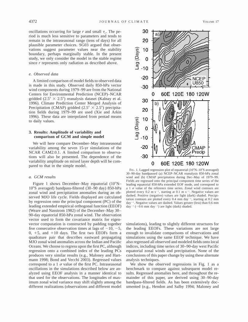
FIG. 1. Lagged regression plot of equatorial (108N–108S averaged)30–90-day bandpassed (a) NCEP–NCAR reanalysis 850-hPa zonalwind and (b) CMAP precipitation during Dec–May of 1979–99.Fields are regressed onto the principal component time series of theleading equatorial 850-hPa extended EOF mode, and correspond toa 1 s value of the reference time series. Zonal wind contours areplotted every 0.2 m s21, starting at 0.1 m s21. Negative values aredashed. Positive (negative) values are light (dark) shaded. Precipi-tation contours are plotted every 0.4 mm day21, starting at 0.2 mmday21. Negative values are dashed. Values greater (less) than 0.6 mmday21 (20.6 mm day21) are light (dark) shaded.
oscillations occurring for large r and small tc. The pe-riod is much less sensitive to parameters and tends toremain in the intraseasonal range (tens of days) for allplausible parameter choices. SG03 argued that obser-vations suggest parameter values near the stabilityboundary, perhaps marginally stable. In the presentstudy, we only consider the model in the stable regimesince r represents only radiation as described above.
e. Observed data
A limited comparison of model fields to observed datais made in this study. Observed daily 850-hPa vectorwind components during 1979–99 are from the NationalCenters for Environmental Prediction (NCEP)–NCARgridded (2.58 3 2.58) reanalysis dataset (Kalnay et al.1996). Climate Prediction Center Merged Analysis ofPrecipitation (CMAP) gridded (2.58 3 2.58) precipita-tion fields during 1979–99 are used (Xie and Arkin1996). These data are interpolated from pentad meansto daily values.
3. Results: Amplitude of variability andcomparison of GCM and simple model
We will here compare December–May intraseasonalvariability among the seven 15-yr simulations of theNCAR CAM2.0.1. A limited comparison to observa-tions will also be presented. The dependence of thevariability amplitude on mixed layer depth will be com-pared to that in the simple model.
a. GCM results
Figure 1 shows December–May equatorial (108N–108S averaged) bandpass-filtered (30–90 day) 850-hPazonal wind and precipitation anomalies during an ob-served MJO life cycle. Fields displayed are calculatedby regression onto the principal component (PC) of theleading extended empirical orthogonal function (EEOF)(Weare and Nasstrom 1982) of the December–May 30–90-day equatorial 850-hPa zonal wind. The observationvector used to form the covariance matrix for eigen-vector computation is constructed by padding togetherfive consecutive observation times at lags of 210, 25,0, 15, and 110 days. The first two EEOFs form aquadrature pair that describes eastward propagatingMJO zonal wind anomalies across the Indian and PacificOceans. We choose to regress upon the first PC, althoughregression onto a combined index of the leading PCsproduces very similar results (e.g., Maloney and Hart-mann 1998; Bond and Vecchi 2003). Regressed valuescorrespond to a 1 s value of the first PC. Intraseasonaloscillations in the simulations described below are an-alyzed using EEOF analysis in a manner identical tothat used for the observations. The longitudes of max-imum zonal wind variance may shift slightly among thedifferent realizations (observations and different model
simulations), leading to slightly different structures forthe leading EEOFs. These variations are not largeenough to invalidate comparisons of observations andsimulations using the same EEOF technique. We havealso regressed all observed and modeled fields onto localindices, including time series of 30–90-day west Pacificequatorial zonal winds and precipitation. None of theconclusions of this paper change by using these alternateanalysis techniques.
We show the observed regressions in Fig. 1 as abenchmark to compare against subsequent model re-sults. Regressed anomalies here, and throughout the re-mainder of this paper, are derived using 30–90-daybandpass-filtered fields. As has been extensively doc-umented (e.g., Hendon and Salby 1994; Maloney and
15 NOVEMBER 2004 4373M A L O N E Y A N D S O B E L
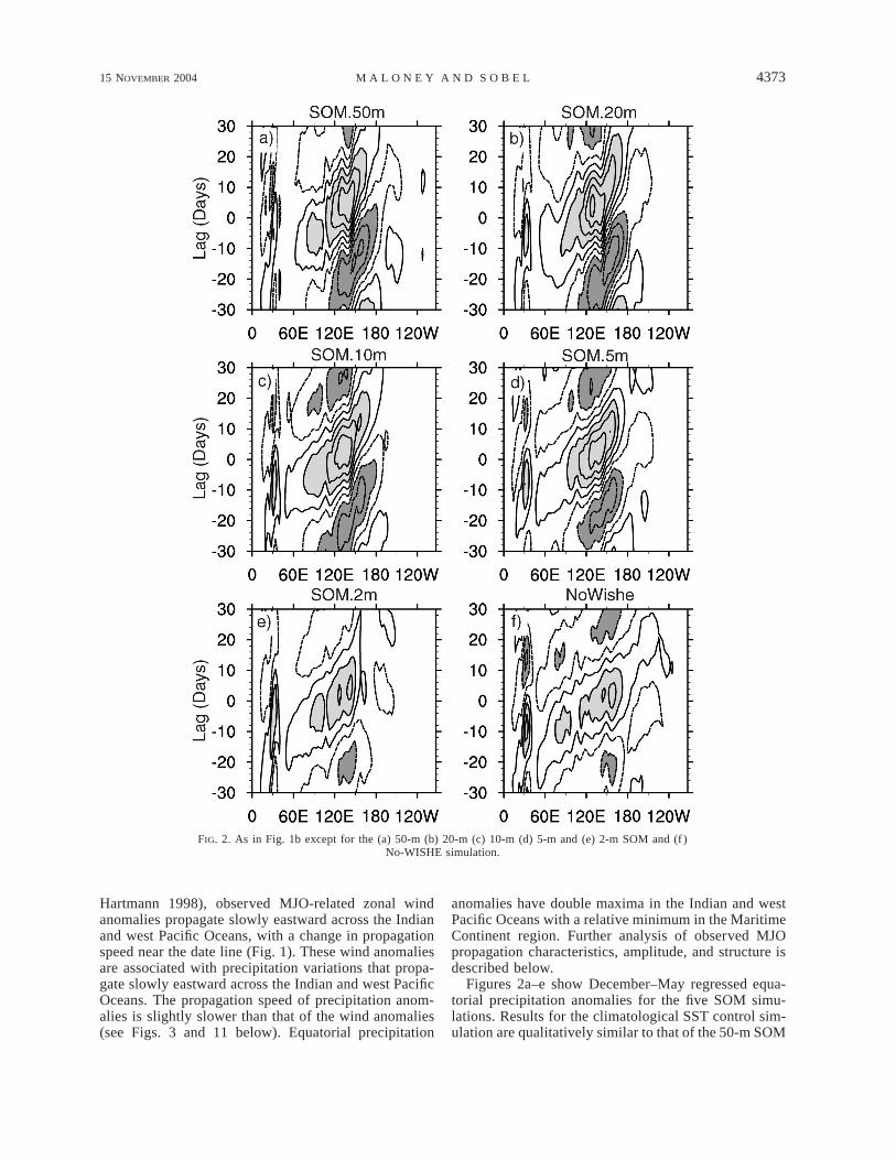
FIG. 2. As in Fig. 1b except for the (a) 50-m (b) 20-m (c) 10-m (d) 5-m and (e) 2-m SOM and (f )No-WISHE simulation.
Hartmann 1998), observed MJO-related zonal windanomalies propagate slowly eastward across the Indianand west Pacific Oceans, with a change in propagationspeed near the date line (Fig. 1). These wind anomaliesare associated with precipitation variations that propa-gate slowly eastward across the Indian and west PacificOceans. The propagation speed of precipitation anom-alies is slightly slower than that of the wind anomalies(see Figs. 3 and 11 below). Equatorial precipitation
anomalies have double maxima in the Indian and westPacific Oceans with a relative minimum in the MaritimeContinent region. Further analysis of observed MJOpropagation characteristics, amplitude, and structure isdescribed below.
Figures 2a–e show December–May regressed equa-torial precipitation anomalies for the five SOM simu-lations. Results for the climatological SST control sim-ulation are qualitatively similar to that of the 50-m SOM
4374 VOLUME 17J O U R N A L O F C L I M A T E
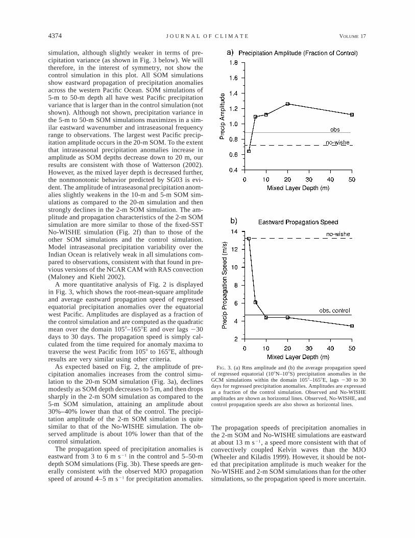
FIG. 3. (a) Rms amplitude and (b) the average propagation speedof regressed equatorial (108N–108S) precipitation anomalies in theGCM simulations within the domain 1058–1658E, lags 230 to 30days for regressed precipitation anomalies. Amplitudes are expressedas a fraction of the control simulation. Observed and No-WISHEamplitudes are shown as horizontal lines. Observed, No-WISHE, andcontrol propagation speeds are also shown as horizontal lines.
simulation, although slightly weaker in terms of pre-cipitation variance (as shown in Fig. 3 below). We willtherefore, in the interest of symmetry, not show thecontrol simulation in this plot. All SOM simulationsshow eastward propagation of precipitation anomaliesacross the western Pacific Ocean. SOM simulations of5-m to 50-m depth all have west Pacific precipitationvariance that is larger than in the control simulation (notshown). Although not shown, precipitation variance inthe 5-m to 50-m SOM simulations maximizes in a sim-ilar eastward wavenumber and intraseasonal frequencyrange to observations. The largest west Pacific precip-itation amplitude occurs in the 20-m SOM. To the extentthat intraseasonal precipitation anomalies increase inamplitude as SOM depths decrease down to 20 m, ourresults are consistent with those of Watterson (2002).However, as the mixed layer depth is decreased further,the nonmonotonic behavior predicted by SG03 is evi-dent. The amplitude of intraseasonal precipitation anom-alies slightly weakens in the 10-m and 5-m SOM sim-ulations as compared to the 20-m simulation and thenstrongly declines in the 2-m SOM simulation. The am-plitude and propagation characteristics of the 2-m SOMsimulation are more similar to those of the fixed-SSTNo-WISHE simulation (Fig. 2f) than to those of theother SOM simulations and the control simulation.Model intraseasonal precipitation variability over theIndian Ocean is relatively weak in all simulations com-pared to observations, consistent with that found in pre-vious versions of the NCAR CAM with RAS convection(Maloney and Kiehl 2002).
A more quantitative analysis of Fig. 2 is displayedin Fig. 3, which shows the root-mean-square amplitudeand average eastward propagation speed of regressedequatorial precipitation anomalies over the equatorialwest Pacific. Amplitudes are displayed as a fraction ofthe control simulation and are computed as the quadraticmean over the domain 1058–1658E and over lags 230days to 30 days. The propagation speed is simply cal-culated from the time required for anomaly maxima totraverse the west Pacific from 1058 to 1658E, althoughresults are very similar using other criteria.
As expected based on Fig. 2, the amplitude of pre-cipitation anomalies increases from the control simu-lation to the 20-m SOM simulation (Fig. 3a), declinesmodestly as SOM depth decreases to 5 m, and then dropssharply in the 2-m SOM simulation as compared to the5-m SOM simulation, attaining an amplitude about30%–40% lower than that of the control. The precipi-tation amplitude of the 2-m SOM simulation is quitesimilar to that of the No-WISHE simulation. The ob-served amplitude is about 10% lower than that of thecontrol simulation.
The propagation speed of precipitation anomalies iseastward from 3 to 6 m s21 in the control and 5–50-mdepth SOM simulations (Fig. 3b). These speeds are gen-erally consistent with the observed MJO propagationspeed of around 4–5 m s21 for precipitation anomalies.
The propagation speeds of precipitation anomalies inthe 2-m SOM and No-WISHE simulations are eastwardat about 13 m s21, a speed more consistent with that ofconvectively coupled Kelvin waves than the MJO(Wheeler and Kiladis 1999). However, it should be not-ed that precipitation amplitude is much weaker for theNo-WISHE and 2-m SOM simulations than for the othersimulations, so the propagation speed is more uncertain.
15 NOVEMBER 2004 4375M A L O N E Y A N D S O B E L
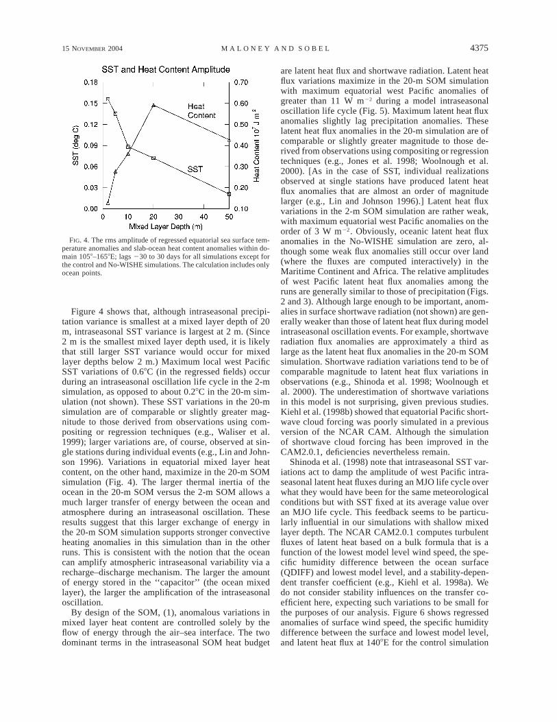
FIG. 4. The rms amplitude of regressed equatorial sea surface tem-perature anomalies and slab-ocean heat content anomalies within do-main 1058–1658E; lags 230 to 30 days for all simulations except forthe control and No-WISHE simulations. The calculation includes onlyocean points.
Figure 4 shows that, although intraseasonal precipi-tation variance is smallest at a mixed layer depth of 20m, intraseasonal SST variance is largest at 2 m. (Since2 m is the smallest mixed layer depth used, it is likelythat still larger SST variance would occur for mixedlayer depths below 2 m.) Maximum local west PacificSST variations of 0.68C (in the regressed fields) occurduring an intraseasonal oscillation life cycle in the 2-msimulation, as opposed to about 0.28C in the 20-m sim-ulation (not shown). These SST variations in the 20-msimulation are of comparable or slightly greater mag-nitude to those derived from observations using com-positing or regression techniques (e.g., Waliser et al.1999); larger variations are, of course, observed at sin-gle stations during individual events (e.g., Lin and John-son 1996). Variations in equatorial mixed layer heatcontent, on the other hand, maximize in the 20-m SOMsimulation (Fig. 4). The larger thermal inertia of theocean in the 20-m SOM versus the 2-m SOM allows amuch larger transfer of energy between the ocean andatmosphere during an intraseasonal oscillation. Theseresults suggest that this larger exchange of energy inthe 20-m SOM simulation supports stronger convectiveheating anomalies in this simulation than in the otherruns. This is consistent with the notion that the oceancan amplify atmospheric intraseasonal variability via arecharge–discharge mechanism. The larger the amountof energy stored in the ‘‘capacitor’’ (the ocean mixedlayer), the larger the amplification of the intraseasonaloscillation.
By design of the SOM, (1), anomalous variations inmixed layer heat content are controlled solely by theflow of energy through the air–sea interface. The twodominant terms in the intraseasonal SOM heat budget
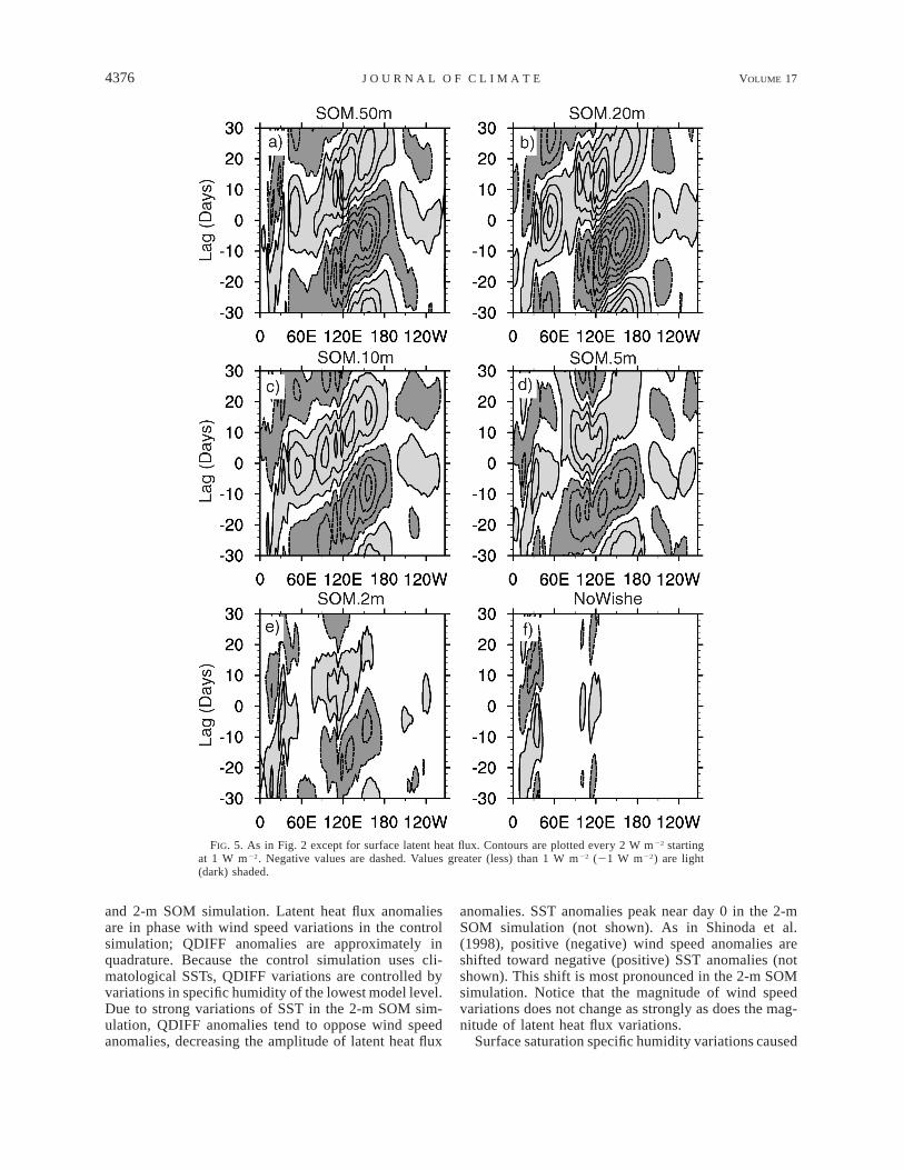
are latent heat flux and shortwave radiation. Latent heatflux variations maximize in the 20-m SOM simulationwith maximum equatorial west Pacific anomalies ofgreater than 11 W m22 during a model intraseasonaloscillation life cycle (Fig. 5). Maximum latent heat fluxanomalies slightly lag precipitation anomalies. Theselatent heat flux anomalies in the 20-m simulation are ofcomparable or slightly greater magnitude to those de-rived from observations using compositing or regressiontechniques (e.g., Jones et al. 1998; Woolnough et al.2000). [As in the case of SST, individual realizationsobserved at single stations have produced latent heatflux anomalies that are almost an order of magnitudelarger (e.g., Lin and Johnson 1996).] Latent heat fluxvariations in the 2-m SOM simulation are rather weak,with maximum equatorial west Pacific anomalies on theorder of 3 W m22. Obviously, oceanic latent heat fluxanomalies in the No-WISHE simulation are zero, al-though some weak flux anomalies still occur over land(where the fluxes are computed interactively) in theMaritime Continent and Africa. The relative amplitudesof west Pacific latent heat flux anomalies among theruns are generally similar to those of precipitation (Figs.2 and 3). Although large enough to be important, anom-alies in surface shortwave radiation (not shown) are gen-erally weaker than those of latent heat flux during modelintraseasonal oscillation events. For example, shortwaveradiation flux anomalies are approximately a third aslarge as the latent heat flux anomalies in the 20-m SOMsimulation. Shortwave radiation variations tend to be ofcomparable magnitude to latent heat flux variations inobservations (e.g., Shinoda et al. 1998; Woolnough etal. 2000). The underestimation of shortwave variationsin this model is not surprising, given previous studies.Kiehl et al. (1998b) showed that equatorial Pacific short-wave cloud forcing was poorly simulated in a previousversion of the NCAR CAM. Although the simulationof shortwave cloud forcing has been improved in theCAM2.0.1, deficiencies nevertheless remain.
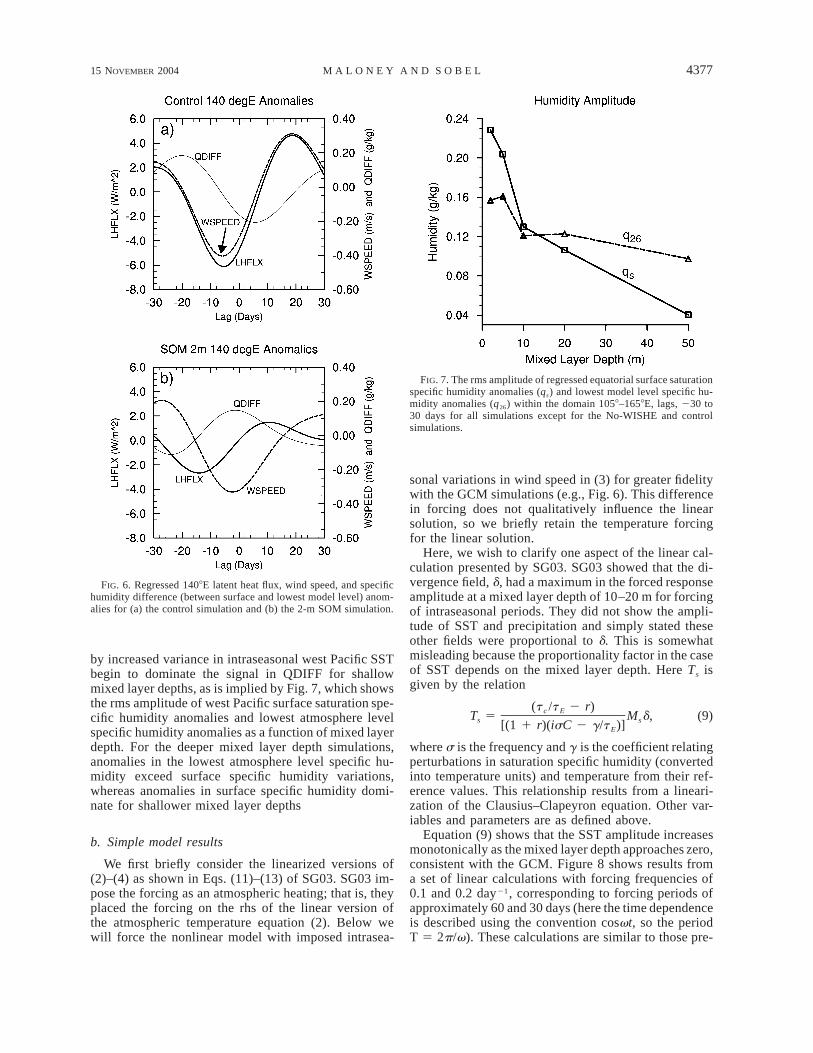
Shinoda et al. (1998) note that intraseasonal SST var-iations act to damp the amplitude of west Pacific intra-seasonal latent heat fluxes during an MJO life cycle overwhat they would have been for the same meteorologicalconditions but with SST fixed at its average value overan MJO life cycle. This feedback seems to be particu-larly influential in our simulations with shallow mixedlayer depth. The NCAR CAM2.0.1 computes turbulentfluxes of latent heat based on a bulk formula that is afunction of the lowest model level wind speed, the spe-cific humidity difference between the ocean surface(QDIFF) and lowest model level, and a stability-depen-dent transfer coefficient (e.g., Kiehl et al. 1998a). Wedo not consider stability influences on the transfer co-efficient here, expecting such variations to be small forthe purposes of our analysis. Figure 6 shows regressedanomalies of surface wind speed, the specific humiditydifference between the surface and lowest model level,and latent heat flux at 1408E for the control simulation
4376 VOLUME 17J O U R N A L O F C L I M A T E
FIG. 5. As in Fig. 2 except for surface latent heat flux. Contours are plotted every 2 W m22 startingat 1 W m22. Negative values are dashed. Values greater (less) than 1 W m22 (21 W m22) are light(dark) shaded.
and 2-m SOM simulation. Latent heat flux anomaliesare in phase with wind speed variations in the controlsimulation; QDIFF anomalies are approximately inquadrature. Because the control simulation uses cli-matological SSTs, QDIFF variations are controlled byvariations in specific humidity of the lowest model level.Due to strong variations of SST in the 2-m SOM sim-ulation, QDIFF anomalies tend to oppose wind speedanomalies, decreasing the amplitude of latent heat flux
anomalies. SST anomalies peak near day 0 in the 2-mSOM simulation (not shown). As in Shinoda et al.(1998), positive (negative) wind speed anomalies areshifted toward negative (positive) SST anomalies (notshown). This shift is most pronounced in the 2-m SOMsimulation. Notice that the magnitude of wind speedvariations does not change as strongly as does the mag-nitude of latent heat flux variations.
Surface saturation specific humidity variations caused
15 NOVEMBER 2004 4377M A L O N E Y A N D S O B E L
FIG. 6. Regressed 1408E latent heat flux, wind speed, and specifichumidity difference (between surface and lowest model level) anom-alies for (a) the control simulation and (b) the 2-m SOM simulation.
FIG. 7. The rms amplitude of regressed equatorial surface saturationspecific humidity anomalies (qs) and lowest model level specific hu-midity anomalies (q26) within the domain 1058–1658E, lags, 230 to30 days for all simulations except for the No-WISHE and controlsimulations.
by increased variance in intraseasonal west Pacific SSTbegin to dominate the signal in QDIFF for shallowmixed layer depths, as is implied by Fig. 7, which showsthe rms amplitude of west Pacific surface saturation spe-cific humidity anomalies and lowest atmosphere levelspecific humidity anomalies as a function of mixed layerdepth. For the deeper mixed layer depth simulations,anomalies in the lowest atmosphere level specific hu-midity exceed surface specific humidity variations,whereas anomalies in surface specific humidity domi-nate for shallower mixed layer depths
b. Simple model results
We first briefly consider the linearized versions of(2)–(4) as shown in Eqs. (11)–(13) of SG03. SG03 im-pose the forcing as an atmospheric heating; that is, theyplaced the forcing on the rhs of the linear version ofthe atmospheric temperature equation (2). Below wewill force the nonlinear model with imposed intrasea-
sonal variations in wind speed in (3) for greater fidelitywith the GCM simulations (e.g., Fig. 6). This differencein forcing does not qualitatively influence the linearsolution, so we briefly retain the temperature forcingfor the linear solution.
Here, we wish to clarify one aspect of the linear cal-culation presented by SG03. SG03 showed that the di-vergence field, d, had a maximum in the forced responseamplitude at a mixed layer depth of 10–20 m for forcingof intraseasonal periods. They did not show the ampli-tude of SST and precipitation and simply stated theseother fields were proportional to d. This is somewhatmisleading because the proportionality factor in the caseof SST depends on the mixed layer depth. Here Ts isgiven by the relation
(t /t 2 r)c ET 5 M d, (9)s s[(1 1 r)(isC 2 g/t )]E
where s is the frequency and g is the coefficient relatingperturbations in saturation specific humidity (convertedinto temperature units) and temperature from their ref-erence values. This relationship results from a lineari-zation of the Clausius–Clapeyron equation. Other var-iables and parameters are as defined above.
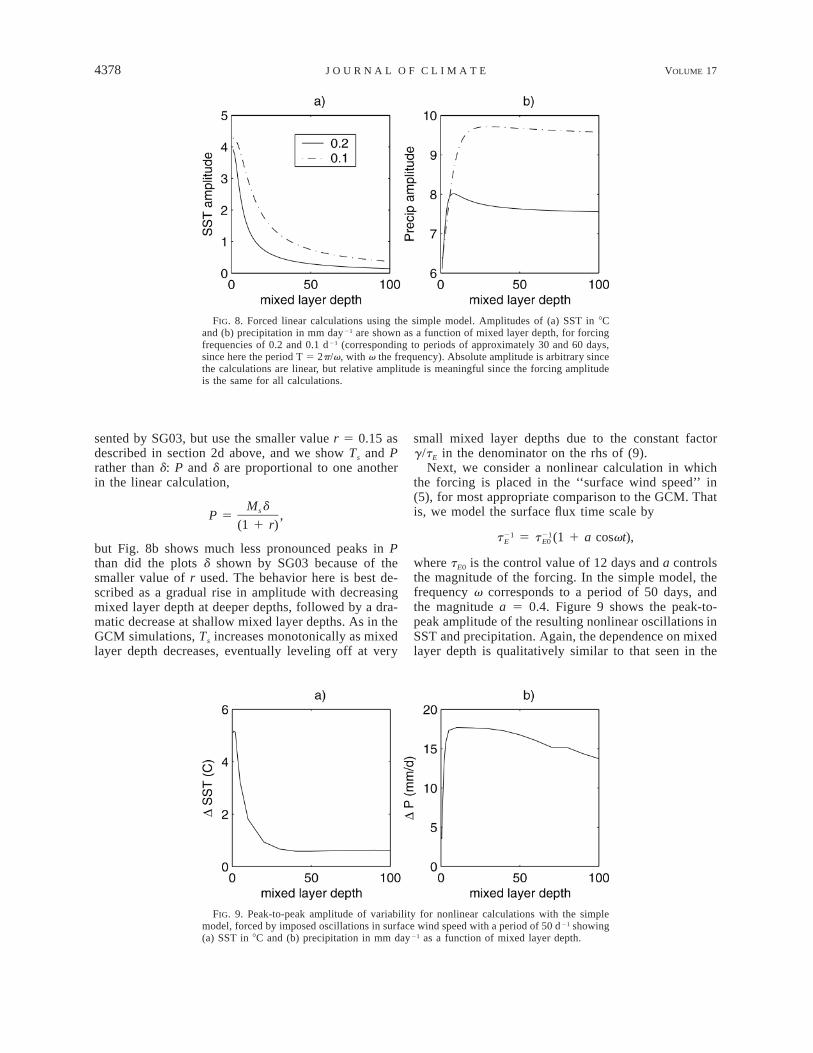
Equation (9) shows that the SST amplitude increasesmonotonically as the mixed layer depth approaches zero,consistent with the GCM. Figure 8 shows results froma set of linear calculations with forcing frequencies of0.1 and 0.2 day21, corresponding to forcing periods ofapproximately 60 and 30 days (here the time dependenceis described using the convention cosvt, so the periodT 5 2p/v). These calculations are similar to those pre-
4378 VOLUME 17J O U R N A L O F C L I M A T E
FIG. 8. Forced linear calculations using the simple model. Amplitudes of (a) SST in 8Cand (b) precipitation in mm day21 are shown as a function of mixed layer depth, for forcingfrequencies of 0.2 and 0.1 d21 (corresponding to periods of approximately 30 and 60 days,since here the period T 5 2p/v, with v the frequency). Absolute amplitude is arbitrary sincethe calculations are linear, but relative amplitude is meaningful since the forcing amplitudeis the same for all calculations.
FIG. 9. Peak-to-peak amplitude of variability for nonlinear calculations with the simplemodel, forced by imposed oscillations in surface wind speed with a period of 50 d21 showing(a) SST in 8C and (b) precipitation in mm day21 as a function of mixed layer depth.
sented by SG03, but use the smaller value r 5 0.15 asdescribed in section 2d above, and we show Ts and Prather than d: P and d are proportional to one anotherin the linear calculation,
M dsP 5 ,(1 1 r)
but Fig. 8b shows much less pronounced peaks in Pthan did the plots d shown by SG03 because of thesmaller value of r used. The behavior here is best de-scribed as a gradual rise in amplitude with decreasingmixed layer depth at deeper depths, followed by a dra-matic decrease at shallow mixed layer depths. As in theGCM simulations, Ts increases monotonically as mixedlayer depth decreases, eventually leveling off at very
small mixed layer depths due to the constant factorg/tE in the denominator on the rhs of (9).
Next, we consider a nonlinear calculation in whichthe forcing is placed in the ‘‘surface wind speed’’ in(5), for most appropriate comparison to the GCM. Thatis, we model the surface flux time scale by
21 21t 5 t (1 1 a cosvt),E E0
where tE0 is the control value of 12 days and a controlsthe magnitude of the forcing. In the simple model, thefrequency v corresponds to a period of 50 days, andthe magnitude a 5 0.4. Figure 9 shows the peak-to-peak amplitude of the resulting nonlinear oscillations inSST and precipitation. Again, the dependence on mixedlayer depth is qualitatively similar to that seen in the
15 NOVEMBER 2004 4379M A L O N E Y A N D S O B E L
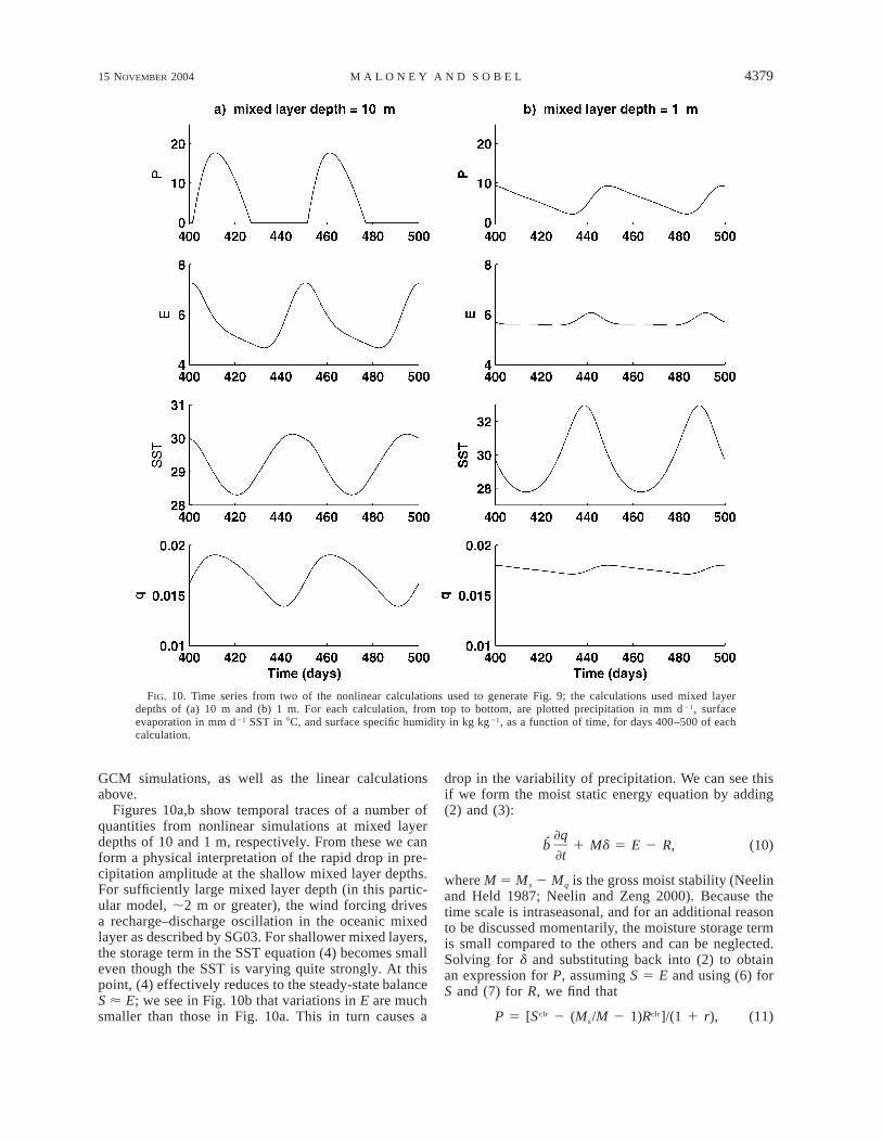
FIG. 10. Time series from two of the nonlinear calculations used to generate Fig. 9; the calculations used mixed layerdepths of (a) 10 m and (b) 1 m. For each calculation, from top to bottom, are plotted precipitation in mm d21, surfaceevaporation in mm d21 SST in 8C, and surface specific humidity in kg kg21, as a function of time, for days 400–500 of eachcalculation.
GCM simulations, as well as the linear calculationsabove.
Figures 10a,b show temporal traces of a number ofquantities from nonlinear simulations at mixed layerdepths of 10 and 1 m, respectively. From these we canform a physical interpretation of the rapid drop in pre-cipitation amplitude at the shallow mixed layer depths.For sufficiently large mixed layer depth (in this partic-ular model, ;2 m or greater), the wind forcing drivesa recharge–discharge oscillation in the oceanic mixedlayer as described by SG03. For shallower mixed layers,the storage term in the SST equation (4) becomes smalleven though the SST is varying quite strongly. At thispoint, (4) effectively reduces to the steady-state balanceS ø E; we see in Fig. 10b that variations in E are muchsmaller than those in Fig. 10a. This in turn causes a
drop in the variability of precipitation. We can see thisif we form the moist static energy equation by adding(2) and (3):
]qb̂ 1 Md 5 E 2 R, (10)
]t
where M 5 Ms 2 Mq is the gross moist stability (Neelinand Held 1987; Neelin and Zeng 2000). Because thetime scale is intraseasonal, and for an additional reasonto be discussed momentarily, the moisture storage termis small compared to the others and can be neglected.Solving for d and substituting back into (2) to obtainan expression for P, assuming S 5 E and using (6) forS and (7) for R, we find that
clr clrP 5 [S 2 (M /M 2 1)R ]/(1 1 r),s (11)
4380 VOLUME 17J O U R N A L O F C L I M A T E
which shows that precipitation is constant in this limit.Accordingly, we see that the precipitation varies muchless for a 1-m SOM than for a 10-m SOM. In fact, the10-m SOM has periods of zero precipitation, but the 1-m SOM does not. If precipitation is nonzero at all times,a strong constraint is placed on the moisture field, q.During periods when P . 0, the Betts–Miller scheme(5) relaxes q strongly toward T, which is constant byWTG. If there are periods of zero precipitation, thenduring those periods q does not feel this constraint, andcan vary more. Thus, we see much smaller q variationsin Fig. 10b than in 10a. This helps to justify our neglectof the tendency term in the above discussion.
The end result of this argument is that, in the shallowmixed layer case, q and E are both approximately heldto constant values while the wind speed varies in aprescribed way. The only possibility then is for toq*svary by changing SST within the constraints providedby the other three variables in (6). In other words, SSTmust vary in such a way as to reduce surface latent heatflux variations.
The GCM results are qualitatively consistent withthese simple model results. The essential mechanism ofthe precipitation variance reduction at small mixed layerdepth is the same in both models. We see the strongreduction in surface evaporation variations in the 2-mGCM simulation in Fig. 5. On the other hand, the mixedlayer depth dependence of the surface air humidity inthe GCM (Fig. 7) is not entirely consistent with thesimple model’s behavior. The variance in surface airhumidity increases monotonically as mixed layer depthdecreases, whereas in the simple model the former de-creases as the latter reaches very small values. None-theless, the surface air humidity variance increases moreslowly than does the variance saturation humidity of thesea surface in the GCM. This presumably indicates someregulation of the surface air humidity by deep convec-tion (despite the lack of parameterized downdrafts inthe convection scheme), as in the simple model. In bothmodels, the SST responds to keep surface evaporationvariations small in the face of large surface wind var-iations and constrained surface air humidity variations.
To some degree, the reduction in amplitude (both inthe GCM and simple model) as the mixed layer becomesvery shallow should be expected, given that the vari-ability depends on energy exchange between the at-mosphere and ocean. In the ‘‘swamp’’ limit (zero mixedlayer depth), there can be no energy exchange. Neelinet al. (1987) showed in a GCM simulation that theWISHE mechanism was rendered inoperative in theswamp limit. The most important new result here, per-haps, is the explicit demonstration that neither the fixed-SST nor the swamp limits yields the maximum ampli-tude, but rather that the maximum occurs near the ob-served mixed layer depth in the regions where the MJOis active.
c. Discussion: Relevance to observations
Our simple SOM with fixed, uniform mixed layerdepth is a primitive substitute for the real ocean. Weview our sensitivity tests with this model, in which themixed layer depth is varied, as valuable primarily forthe insight they give us into the coupled MJO dynamicsin the GCM. It is difficult to imagine a fully convincingobservational test of the above results since the dramaticdependence of precipitation variability on mixed layerdepth only occurs at mixed layer depths of a few metersor less, smaller than those ever (to our knowledge) ob-served in the ocean regions where the MJO is active.However, wet land is somewhat like a very shallowocean mixed layer in that it has minimal heat capacityand a small Bowen ratio. The dependence on mixedlayer depth found here may help explain the local min-imum in MJO amplitude that is observed in the MaritimeContinent. During austral summer when the MJO ismost active, it is the rainy season over the MaritimeContinent and the landmasses are presumably fairly wet.The land may be considered comparable to a very shal-low mixed layer, which our simulations suggest shouldlead to a drop in MJO amplitude.
This does not preclude that other factors may con-tribute to the local amplitude minimum, such as thetopography associated with the Indonesian mountainranges or the strong diurnal component of convectionover land (e.g., Zhang and Hendon 1997). (The strongdiurnal cycle over land is actually closely related to themechanism that we described for the weakening of theMJO. The diurnal cycle is also a forced recharge–dis-charge oscillation. Land has small heat capacity, so thehigh-frequency diurnal cycle is strong while the low-frequency MJO is weak.) We would like to test theseideas in future work, for example, by performing GCMsimulations in which the Indonesian islands are retained,but with their surface elevations set to zero. Unfortu-nately, the GCM used here is not ideal for these studies;its amplitude minimum is not particularly well defineddue to unrealistically weak MJO variability in the IndianOcean (e.g., Fig. 2).
4. Results: Zonal wind and horizontal structure inthe GCM simulations
Interestingly, equatorial zonal wind variability exhib-its somewhat different behavior than precipitation var-iability among the model simulations. Figure 11 showsthe same quantitative analysis of equatorial amplitudeand propagation speed as in Fig. 3 except for 850-hPazonal wind. Zonal wind anomalies in the SOM simu-lation and No-WISHE simulations are either slightlylarger or similar to those in the control simulation. Al-though precipitation anomalies in the 2-m SOM and No-WISHE simulations are much weaker than the control(Fig. 3), the same is not true of zonal wind anomalies.All simulations have stronger than observed zonal wind
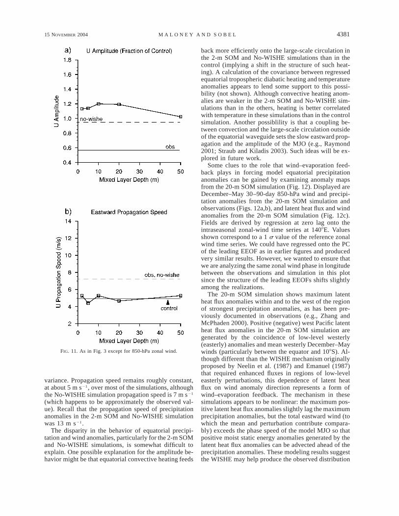
15 NOVEMBER 2004 4381M A L O N E Y A N D S O B E L
FIG. 11. As in Fig. 3 except for 850-hPa zonal wind.
variance. Propagation speed remains roughly constant,at about 5 m s21, over most of the simulations, althoughthe No-WISHE simulation propagation speed is 7 m s21
(which happens to be approximately the observed val-ue). Recall that the propagation speed of precipitationanomalies in the 2-m SOM and No-WISHE simulationwas 13 m s21.
The disparity in the behavior of equatorial precipi-tation and wind anomalies, particularly for the 2-m SOMand No-WISHE simulations, is somewhat difficult toexplain. One possible explanation for the amplitude be-havior might be that equatorial convective heating feeds
back more efficiently onto the large-scale circulation inthe 2-m SOM and No-WISHE simulations than in thecontrol (implying a shift in the structure of such heat-ing). A calculation of the covariance between regressedequatorial tropospheric diabatic heating and temperatureanomalies appears to lend some support to this possi-bility (not shown). Although convective heating anom-alies are weaker in the 2-m SOM and No-WISHE sim-ulations than in the others, heating is better correlatedwith temperature in these simulations than in the controlsimulation. Another possiblility is that a coupling be-tween convection and the large-scale circulation outsideof the equatorial waveguide sets the slow eastward prop-agation and the amplitude of the MJO (e.g., Raymond2001; Straub and Kiladis 2003). Such ideas will be ex-plored in future work.
Some clues to the role that wind–evaporation feed-back plays in forcing model equatorial precipitationanomalies can be gained by examining anomaly mapsfrom the 20-m SOM simulation (Fig. 12). Displayed areDecember–May 30–90-day 850-hPa wind and precipi-tation anomalies from the 20-m SOM simulation andobservations (Figs. 12a,b), and latent heat flux and windanomalies from the 20-m SOM simulation (Fig. 12c).Fields are derived by regression at zero lag onto theintraseasonal zonal-wind time series at 1408E. Valuesshown correspond to a 1 s value of the reference zonalwind time series. We could have regressed onto the PCof the leading EEOF as in earlier figures and producedvery similar results. However, we wanted to ensure thatwe are analyzing the same zonal wind phase in longitudebetween the observations and simulation in this plotsince the structure of the leading EEOFs shifts slightlyamong the realizations.
The 20-m SOM simulation shows maximum latentheat flux anomalies within and to the west of the regionof strongest precipitation anomalies, as has been pre-viously documented in observations (e.g., Zhang andMcPhaden 2000). Positive (negative) west Pacific latentheat flux anomalies in the 20-m SOM simulation aregenerated by the coincidence of low-level westerly(easterly) anomalies and mean westerly December–Maywinds (particularly between the equator and 108S). Al-though different than the WISHE mechanism originallyproposed by Neelin et al. (1987) and Emanuel (1987)that required enhanced fluxes in regions of low-leveleasterly perturbations, this dependence of latent heatflux on wind anomaly direction represents a form ofwind–evaporation feedback. The mechanism in thesesimulations appears to be nonlinear: the maximum pos-itive latent heat flux anomalies slightly lag the maximumprecipitation anomalies, but the total eastward wind (towhich the mean and perturbation contribute compara-bly) exceeds the phase speed of the model MJO so thatpositive moist static energy anomalies generated by thelatent heat flux anomalies can be advected ahead of theprecipitation anomalies. These modeling results suggestthe WISHE may help produce the observed distribution
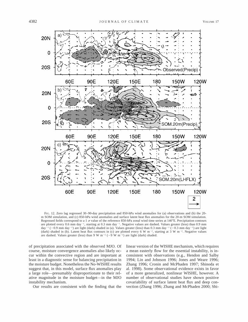
4382 VOLUME 17J O U R N A L O F C L I M A T E
FIG. 12. Zero lag regressed 30–90-day precipitation and 850-hPa wind anomalies for (a) observations and (b) the 20-m SOM simulation, and (c) 850-hPa wind anomalies and surface latent heat flux anomalies for the 20-m SOM simulation.Regressed fields correspond to a 1 s value of the reference 850-hPa zonal wind time series at 1408E. Precipitation contoursare plotted every 0.6 mm day21, starting at 0.3 mm day21. Negative values are dashed. Values greater (less) than 0.9 mmday21 (20.9 mm day21) are light (dark) shaded in (a). Values greater (less) than 0.3 mm day21 (20.3 mm day21) are light(dark) shaded in (b). Latent heat flux contours in (c) are plotted every 6 W m22, starting at 3 W m22. Negative valuesare dashed. Values greater (less) than 9 W m22 (29 W m22) are light (dark) shaded.
of precipitation associated with the observed MJO. Ofcourse, moisture convergence anomalies also likely oc-cur within the convective region and are important atleast in a diagnostic sense for balancing precipitation inthe moisture budget. Nonetheless the No-WISHE resultssuggest that, in this model, surface flux anomalies playa large role—presumably disproportionate to their rel-ative magnitude in the moisture budget—in the MJOinstability mechanism.
Our results are consistent with the finding that the
linear version of the WISHE mechanism, which requiresa mean easterly flow for the essential instability, is in-consistent with observations (e.g., Hendon and Salby1994; Lin and Johnson 1996; Jones and Weare 1996;Zhang 1996; Cronin and McPhaden 1997; Shinoda etal. 1998). Some observational evidence exists in favorof a more generalized, nonlinear WISHE, however. Anumber of observational studies have shown positivecovariability of surface latent heat flux and deep con-vection (Zhang 1996; Zhang and McPhaden 2000; Shi-
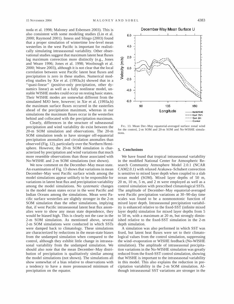
15 NOVEMBER 2004 4383M A L O N E Y A N D S O B E L
FIG. 13. Mean Dec–May equatorial-averaged surface zonal windfor the control, 2-m SOM and 20-m SOM and No-WISHE simula-tions.
noda et al. 1998; Maloney and Esbensen 2003). This isalso consistent with some modeling studies (Lin et al.2000; Raymond 2001). Inness and Slingo (2003) foundthat a proper simulation of wintertime low-level meanwesterlies in the west Pacific is important for realisti-cally simulating intraseasonal variability. Other obser-vational studies suggest that maximum latent heat fluxeslag maximum convection more distinctly (e.g., Jonesand Weare 1996; Jones et al. 1998; Woolnough et al.2000; Weare 2003), although it is not clear that the localcorrelation between west Pacific latent heat fluxes andprecipitation is zero in these studies. Numerical mod-eling studies by Xie et al. (1993a,b) showed that in a‘‘quasi-linear’’ (positive-only precipitation, other dy-namics linear) as well as a fully nonlinear model, un-stable WISHE modes could occur on resting basic states.Their WISHE modes are somewhat different from thesimulated MJO here, however; in Xie et al. (1993a,b)the maximum surface fluxes occurred in the easterliesahead of the precipitation maximum, whereas in oursimulations the maximum fluxes occur in the westerliesbehind and collocated with the precipitation maximum.
Clearly, differences in the structure of subseasonalprecipitation and wind variability do exist between the20-m SOM simulation and observations. The 20-mSOM simulation tends to have stronger off-equatorialprecipitation anomalies and circulation anomalies thanobserved (Fig. 12), particularly over the Northern Hemi-sphere. However, the 20-m SOM simulation is char-acterized by precipitation and wind variations that muchmore resemble observations than those associated withNo-WISHE and 2-m SOM simulations (not shown).
We now comment on the December–May mean state.An examination of Fig. 13 shows that variations in meanDecember–May west Pacific surface winds among themodel simulations appear unlikely to be responsible forvariations in latent heat flux and precipitation variabilityamong the model simulations. No systematic changesin the model mean states occur in the west Pacific andIndian Oceans among the simulations. Mean west Pa-cific surface westerlies are slightly stronger in the 2-mSOM simulation than the other simulations, implyingthat, if west Pacific intraseasonal latent heat flux anom-alies were to show any mean state dependence, theywould be biased high. This is clearly not the case in the2-m SOM simulation. As mentioned above, several2-m SOM simulations were conducted in which SSTswere damped back to climatology. These simulationsare characterized by reductions in the mean-state biasesfrom the undamped simulation when compared to thecontrol, although they exhibit little change in intrasea-sonal variability from the undamped simulation. Weshould also note that the mean December–May distri-bution of precipitation is qualitatively similar amongthe model simulations (not shown). The simulations allshow somewhat of a bias relative to observations witha tendency to have a more pronounced minimum ofprecipitation on the equator.
5. Conclusions
We have found that tropical intraseasonal variabilityin the modified National Center for Atmospheric Re-search Community Atmosphere Model 2.0.1 (NCARCAM2.0.1) with relaxed Arakawa–Schubert convectionis sensitive to mixed layer depth when coupled to a slabocean model (SOM). Mixed layer depths of 50 m,20 m, 10 m, 5 m, and 2 m were employed as well as acontrol simulation with prescribed climatological SSTs.The amplitude of December–May equatorial-averagedwest Pacific precipitation variations at 30–90-day timescales was found to be a nonmonotonic function ofmixed layer depth. Intraseasonal precipitation variabil-ity is enhanced relative to the fixed-SST (infinite mixedlayer depth) simulation for mixed layer depths from 5to 50 m, with a maximum at 20 m, but strongly dimin-ished relative to the fixed-SST simulation in the 2-mdepth simulation.
A simulation was also performed in which SST wasfixed, but latent heat fluxes were set to their climato-logical values from the control simulation, suppressingthe wind–evaporation or WISHE feedback (No-WISHEsimulation). The amplitude of intraseasonal precipita-tion variations in the No-WISHE simulation was greatlyreduced from the fixed-SST control simulation, showingthat WISHE is important to the intraseasonal variabilityin this model. This also explains the reduction in pre-cipitation variability in the 2-m SOM simulation. Al-though intraseasonal SST variations are stronger in the
4384 VOLUME 17J O U R N A L O F C L I M A T E
2-m SOM simulation than in any of the other simula-tions, the surface flux variations are smaller in the 2-mSOM simulations than in any of the others. For intra-seasonal variations, 2 m is close to the ‘‘swamp’’ limitin which WISHE is eliminated, which in this model hasthe effect of weakening equatorial convective variabil-ity. The control simulation and the SOM coupled sim-ulations with mixed layer depths greater than 2 m pro-duce near-equatorial intraseasonal precipitation varia-tions that more closely resemble observations than the2-m or No-WISHE simulations.
The nonmonotonic dependence of precipitation var-iability on mixed layer depth was predicted by SG03using a highly idealized model. Further experiments aredescribed here with the same idealized model, whichhelp to interpret results derived from the modifiedNCAR CAM2.0.1. When the nonlinear SG03 model isplaced in a stable regime and forced with intraseasonalsurface wind speed variations, changing the mixed layerdepth has an effect very similar to that in the GCM withregard to both the amplitude and the structure of thevariability.
This study has been an exercise in understanding thedynamics of the simulated MJO more than an attempt toprove any particular point about the real MJO. Doing thelatter is difficult in GCM studies since different modelsmay (and do) lead to different results. However, we canmake a few suggestions about observed variability:
1) To the extent that exchange of energy between oceanand atmosphere is important to the MJO (whethervia surface fluxes or cloud–radiative effects), the en-hancement to the MJO resulting from ocean couplingcan be expected to maximize at a particular mixedlayer depth. Our results (and those of SG03) suggestthat this depth is close to the observed value in theactive MJO regions, so the real system is close tooptimally tuned for this coupled enhancement to theMJO.
2) We hypothesize that the MJO amplitude minimumin the Maritime Continent region may result fromthe inhibition of the coupled recharge–discharge os-cillation there due to the presence of land, which, ifit is wet, is approximately equivalent to an ocean ofzero depth.
3) A nonlinear version of the WISHE mechanism, oc-curring on a westerly mean state, is important to thesimulated MJO in at least one reasonably state-of-the-art GCM, suggesting that a similar mechanismmay operate in reality.
Acknowledgments. We would like to thank CeciliaBitz for providing the slab ocean model and for relateddiscussions. We would like to thank George Kiladis andWojciech Grabowski for their thorough and insightfulreviews of the manuscript. Xie–Arkin precipitation andNCEP–NCAR reanalysis data were provided by theNOAA–CIRES Climate Diagnostics Center, Boulder,
Colorado. Supercomputing resources were provided bythe National Center for Atmospheric Research, Boulder,Colorado. Eric Maloney was supported by the ClimateDynamics Program of the National Science Foundationunder Grant ATM-0327460. Adam Sobel acknowledgessupport for this work from National Science FoundationGrant DMS-01-39830 and a fellowship from the Davidand Lucile Packard Foundation. Any opinions, findings,conclusions, or recommendations expressed in this pa-per are those of the authors and do not necessarily reflectthe views of the sponsors.
REFERENCES
Bond, N. A., and G. A. Vecchi, 2003: The influence of the Madden–Julian oscillation on precipitation in Oregon and Washington.Wea. Forecasting, 18, 600–613.
Bretherton, C. S., and A. H. Sobel, 2002: A simple model of a con-vectively coupled Walker circulation using the weak temperaturegradient approximation. J. Climate, 15, 2907–2920.
Cronin, M. F., and M. J. McPhaden, 1997: The upper ocean heatbalance in the western equatorial Pacific warm pool during Sep-tember–December 1992. J. Geophys. Res., 102, 27 567–27 587.
Emanuel, K. A., 1987: An air–sea interaction model of intraseasonaloscillations in the tropics. J. Atmos. Sci., 44, 2324–2340.
Fasullo, J., and P. J. Webster, 1999: Warm pool SST variability inrelation to the surface energy balance. J. Climate, 12, 1292–1305.
——, and ——, 2000: Atmospheric and surface variations duringwesterly wind bursts in the tropical western Pacific. Quart. J.Roy. Meteor. Soc., 126, 899–924.
Flatau, M., P. J. Flatau, P. Phoebus, and P. P. Niiler, 1997: The feedbackbetween equatorial convection and local radiative and evapo-rative processes: The implications for intraseasonal oscillations.J. Atmos. Sci., 54, 2373–2386.
Grabowski, W. W., 2003: MJO-like coherent structure: Sensitivitysimulations using the Cloud-Resolving Convection Parameteri-zation (CRCP). J. Atmos. Sci., 60, 847–864.
Gualdi, S., A. Navarra, and M. Fischer, 1999: The tropical intrasea-sonal oscillation in a coupled ocean–atmosphere general circu-lation model. Geophys. Res. Lett., 26, 2973–2976.
Hack, J. J., 1994: Parameterization of moist convection in the Na-tional Center for Atmospheric Research Community ClimateModel (CCM2). J. Geophys. Res., 99, 5551–5568.
Hansen, J., A. Lacis, D. Rind, G. Russell, P. Stone, I. Fung, R. Ruedy,and J. Lerner, 1984: Climate sensitivity: Analysis of feedbackmechanisms in climate processes and sensitivity. Climate Pro-cesses and Climate Sensitivity, Geophys. Monogr., No. 29, Amer.Geophys. Union, 130–163.
Harrison, E. F., P. Minnis, B. R. Barkstrom, V. Ramanathan, R. D.Cess, and G. G. Gibson, 1990: Seasonal variation of cloud-ra-diative forcing derived from the Earth Radiation Budget Ex-periment. J. Geophys. Res., 95, 18 687–18 703.
Hartmann, D. L., L. A. Moy, and Q. Fu, 2001: Tropical convectionand the energy balance at the top of the atmosphere. J. Climate,14, 4495–4511.
Hendon, H. H., and M. L. Salby, 1994: The life cycle of the Madden–Julian oscillation. J. Atmos. Sci., 51, 2225–2237.
——, and J. Glick, 1997: Intraseasonal air–sea interaction in thetropical Indian and Pacific Oceans. J. Climate, 10, 647–661.
Inness, P. M., and J. M. Slingo, 2003: Simulation of the Madden–Julian oscillation in a coupled general circulation model. Part I:Comparison with observations and an atmosphere-only GCM.J. Climate, 16, 345–364.
Jones, C., and B. C. Weare, 1996: The role of low-level moistureconvergence and ocean latent heat fluxes in the Madden–Julian
15 NOVEMBER 2004 4385M A L O N E Y A N D S O B E L
oscillation: An observational analysis using ISCCP data andECMWF analyses. J. Climate, 9, 3086–3104.
——, D. E. Waliser, and C. Gautier, 1998: The influence of the Mad-den–Julian oscillation on ocean surface heat fluxes and sea sur-face temperature. J. Climate, 11, 1057–1072.
Kalnay, E., and Coauthors, 1996: The NCEP/NCAR 40-Year Re-analysis Project. Bull. Amer. Meteor. Soc., 77, 437–471.
Kawamura, R., 1988: Intraseasonal variability of sea surface tem-perature over the tropical western Pacific. J. Meteor. Soc. Japan,66, 1007–1012.
Kemball-Cook, S., B. Wang, and X. Fu, 2002: Simulation of theintraseasonal oscillation in the ECHAM-4 model: The impact ofcoupling with an ocean model. J. Atmos. Sci., 59, 1433–1453.
Kiehl, J. T., 1994: On the observed near cancellation between long-wave and shortwave cloud-forcing in tropical regions. J. Climate,7, 559–565.
——, and P. R. Gent, 2004: The Community Climate System Model,version 2. J. Climate, 17, 3666–3682.
——, J. J. Hack, G. B. Bonan, B. A. Boville, D. L. Williamson, andP. J. Rasch, 1998a: The National Center for Atmospheric Re-search Community Climate Model: CCM3. J. Climate, 11, 1131–1149.
——, ——, and J. W. Hurrell, 1998b: The energy budget of the NCARCommunity Climate Model: CCM3. J. Climate, 11, 1151–1178.
Krishnamurti, T. N., D. K. Oosterhof, and A. V. Mehta, 1988: Air–sea interaction on the time scale of 30–50 days. J. Atmos. Sci.,45, 1304–1322.
Lau, K.-M., and C.-H. Sui, 1997: Mechanisms of short-term sea sur-face temperature regulation: Observations during TOGACOARE. J. Climate, 10, 465–472.
Lee, M. I., I.-S. Kang, J.-M. Kim, and B. E. Mapes, 2001: Influenceof cloud–radiation interaction on simulating the tropical intra-seasonal oscillation in an atmospheric general circulation model.J. Geophys. Res., 106, 14 219–14 233.
Lin, J., and B. E. Mapes, 2004: Radiation budget of the tropicalintraseasonal oscillations. J. Atmos. Sci, 61, 2050–2062.
——, J. D. Neelin, and N. Zeng, 2000: Maintenance of tropical in-traseasonal variability: Impact of wind–evaporation feedbackand midlatitude storms. J. Atmos. Sci., 57, 2793–2823.
Lin, X., and R. H. Johnson, 1996: Kinematic and thermodynamiccharacteristics of the flow over the western Pacific warm poolduring TOGA COARE. J. Atmos. Sci., 53, 695–715.
Lindzen, R. S., and S. Nigam, 1987: On the role of sea surfacetemperature gradients in forcing low-level winds and conver-gence in the tropics. J. Atmos. Sci., 44, 2418–2436.
Madden, R. A., and P. R. Julian, 1994: Observations of the 40–50-day tropical oscillation—A review. Mon. Wea. Rev., 122, 814–837.
Majda, A. J., and R. Klein, 2003: Systematic multiscale models forthe Tropics. J. Atmos. Sci., 60, 393–408.
Maloney, E. D., and D. L. Hartmann, 1998: Frictional moisture con-vergence in a composite life cycle of the Madden–Julian oscil-lation. J. Climate, 11, 2387–2403.
——, and ——, 2001: The sensitivity of intraseasonal variability inthe NCAR CCM3 to changes in convective parameterization. J.Climate, 14, 2015–2034.
——, and J. T. Kiehl, 2002: Intraseasonal eastern Pacific precipitationand SST variations in a GCM coupled to a slab ocean model.J. Climate, 15, 2989–3007.
——, and S. K. Esbensen, 2003: The amplification of east PacificMadden–Julian oscillation convection and wind anomalies dur-ing June–November. J. Climate, 16, 3482–3497.
Moorthi, S., and M. J. Suarez, 1992: Relaxed Arakawa–Schubert: Aparameterization of moist convection for general circulationmodels. Mon. Wea. Rev., 120, 978–1002.
Neelin, J. D., and I. M. Held, 1987: Modeling tropical convergencebased on the moist static energy budget. Mon. Wea. Rev., 115,3–12.
——, and N. Zeng, 2000: A quasi-equilibrium tropical circulationmodel formulation. J. Atmos. Sci., 57, 1741–1766.
——, I. M. Held, and K. H. Cook, 1987: Evaporation–wind feedbackand low-frequency variability in the tropical atmosphere. J. At-mos. Sci., 44, 2341–2348.
Ramanathan, V., R. D. Cess, E. F. Harrison, P. Minnis, B. R. Bark-strom, E. Ahmad, and D. Hartmann, 1989: Cloud-radiative forc-ing and climate: Results from the Earth Radiation Budget Ex-periment. Science, 243, 57–63.
Randall, D., M. Khairoutdinov, A. Arakawa, and W. Grabowski, 2003:Breaking the cloud-parameterization deadlock. Bull. Amer. Me-teor. Soc., 84, 1547–1564.
Raymond, D. J., 2001: A new model of the Madden–Julian oscillation.J. Atmos. Sci., 58, 2807–2819.
Shinoda, T., H. H. Hendon, and J. Glick, 1998: Intraseasonal vari-ability of surface fluxes and sea surface temperatures in thetropical western Pacific and Indian Oceans. J. Climate, 11, 1685–1702.
Sobel, A. H., and C. S. Bretherton, 2000: Modeling tropical precip-itation in a single column. J. Climate, 13, 4378–4392.
——, and H. Gildor, 2003: A simple time-dependent model of SSThotspots. J. Climate, 16, 3978–3992.
——, J. Nilsson, and L. M. Polvani, 2001: The weak temperaturegradient approximation and balanced tropical moisture waves.J. Atmos. Sci., 58, 3650–3665.
Straub, K. H., and G. N. Kiladis, 2003: Interactions between theboreal summer intraseasonal oscillation and higher frequencytropical wave activity. Mon. Wea. Rev., 131, 781–796.
Sud, Y. C., and A. Molod, 1988: The roles of dry convection, cloud–radiation feedback processes and the influence of recent im-provements in the parameterization of convection in the GLAGCM. Mon. Wea. Rev., 116, 2366–2387.
——, G. K. Walker, and K.-M. Lau, 1999: Mechanisms regulatingsea-surface temperatures and deep convection in the tropics.Geophys. Res. Lett., 26, 1019–1022.
Waliser, D. E., 1996: Formation and limiting mechanisms for veryhigh sea surface temperatures: Linking the dynamics and ther-modynamics. J. Climate, 9, 161–188.
——, K. M. Lau, and J.-H. Kim, 1999: The influence of coupled seasurface temperatures on the Madden–Julian oscillation: A modelperturbation experiment. J. Atmos. Sci., 56, 333–358.
Wang, B., and X. Xie, 1998: Coupled modes of the warm pool climatesystem. Part I: The role of air–sea interaction in maintaining theMadden–Julian oscillation. J. Climate, 11, 2116–2135.
Watterson, I. G., 2002: The sensitivity of subannual and intraseasonaltropical variability to model ocean mixed layer depth. J. Geo-phys. Res., 107, 4020, doi:10.1029/2001JD000671.
Weare, B. C., 2003: Composite singular value decomposition analysisof moisture variations associated with the Madden–Julian os-cillation. J. Climate, 16, 3779–3792.
——, and J. S. Nasstrom, 1982: Examples of extended empiricalorthogonal function analysis. Mon. Wea. Rev., 110, 481–485.
Weller, R. A., and S. P. Anderson, 1996: Surface meteorology andair–sea fluxes in the western equatorial Pacific warm pool duringthe TOGA Coupled Ocean–Atmosphere Response Experiment.J. Climate, 9, 1959–1990.
Wheeler, M., and G. N. Kiladis, 1999: Convectively coupled equa-torial waves: Analysis of clouds and temperature in the wave-number–frequency domain. J. Atmos. Sci., 56, 374–399.
Woolnough, S. J., J. M. Slingo, and B. J. Hoskins, 2000: The rela-tionship between convection and sea surface temperatures onintraseasonal timescales. J. Climate, 13, 2086–2104.
Xie, P., and P. A. Arkin, 1996: Analyses of global monthly precipi-tation using gauge observations, satellite estimates, and numer-ical model predictions. J. Climate, 9, 840–858.
Xie, S.-P., A. Kubokawa, and K. Hanawa, 1993a: Evaporation–windfeedback and the organizing of tropical convection on the plan-etary scale. Part I: Quasi-linear instability. J. Atmos. Sci., 50,3873–3883.

4386 VOLUME 17J O U R N A L O F C L I M A T E
——, ——, and ——,1993b: Evaporation–wind feedback and theorganizing of tropical convection on the planetary scale. Part II:Nonlinear evolution. J. Atmos. Sci., 50, 3884–3893.
Zhang, C., 1996: Atmospheric intraseasonal variability at the surface inthe tropical western Pacific Ocean. J. Atmos. Sci., 53, 739–758.
——, and N. A. McFarlane, 1995: Sensitivity of climate simulationsto the parameterization of cumulus convection in the Canadian
Climate Centre General Circulation Model. Atmos.–Ocean, 33,407–446.
——, and H. H. Hendon, 1997: Propagating and standing componentsof the intraseasonal oscillation in tropical convection. J. Atmos.Sci., 54, 741–752.
——, and M. J. McPhaden, 2000: Intraseasonal surface cooling inthe equatorial western Pacific. J. Climate, 13, 2261–2276.