Net ecosystem fluxes of isoprene over tropical South ...difficult especially where ecosystem diversity is high, for example, tropical rainforests. Parameterized variability of isoprene

Net ecosystem fluxes of isoprene over tropical South America

inferred from Global Ozone Monitoring Experiment (GOME)

observations of HCHO columns

Michael P. Barkley,1 Paul I. Palmer,1 Uwe Kuhn,2,3 Juergen Kesselmeier,2

Kelly Chance,4 Thomas P. Kurosu,4 Randall V. Martin,4,5 Detlev Helmig,6

and Alex Guenther7

Received 24 January 2008; revised 17 June 2008; accepted 22 July 2008; published 17 October 2008.

[1] We estimate isoprene emissions over tropical South America during 1997–2001using column measurements of formaldehyde (HCHO) from the Global Ozone MonitoringExperiment (GOME) satellite instrument, the GEOS-Chem chemistry transport model,and the MEGAN (Model of Emissions of Gases and Aerosols from Nature) bottom-upisoprene inventory. GEOS-Chem is qualitatively consistent with in situ ground-basedand aircraft concentration profiles of isoprene and HCHO, and GOME HCHO column data(r = 0.41; bias = +35%), but has less skill in reproducing wet season observations.Observed variability of GOME HCHO columns over South America is determinedlargely by isoprene and biomass burning. We find that the column contributionsfrom other biogenic volatile organic compounds (VOC) are typically smallerthan the column fitting uncertainty. HCHO columns influenced by biomass burningare removed using Along Track Scanning Radiometer (ATSR) firecounts and GOME NO2

columns. We find that South America can be split into eastern and western regions,with fires concentrated over the eastern region. A monthly mean linear transfer function,determined by GEOS-Chem, is used to infer isoprene emissions from observed HCHOcolumns. The seasonal variation of GOME isoprene emissions over the western regionis broadly consistent with MEGAN (r = 0.41; bias = �25%), with largest isopreneemissions during the dry season when the observed variability is consistent with knowledgeof temperature dependence. During the wet season, other unknown factors playa significant role in determining observed variability.

Citation: Barkley, M. P., P. I. Palmer, U. Kuhn, J. Kesselmeier, K. Chance, T. P. Kurosu, R. V. Martin, D. Helmig, and A. Guenther

(2008), Net ecosystem fluxes of isoprene over tropical South America inferred from Global Ozone Monitoring Experiment (GOME)

observations of HCHO columns, J. Geophys. Res., 113, D20304, doi:10.1029/2008JD009863.

1. Introduction

[2] Tropical terrestrial ecosystems are a significant sourceof biogenic volatile organic compounds (BVOCs). Thedominant nonmethane BVOC is isoprene (C5H8), whichrepresents almost half of the global annual nonmethaneVOC flux [Guenther et al., 1995, 2006]. Tropical ecosystemscontribute nearly 75% of the global atmospheric isoprene

budget [Guenther et al., 2006], reflecting a year-longgrowing season, warm temperatures, and high solar insola-tion. The high VOC loading and favorable atmosphericconditions (high concentrations of the hydroxyl radical,OH) ensures that the tropics also exert considerable influ-ence on global tropospheric photochemistry [Andreae andCrutzen, 1997]. Isoprene has a strong influence on theoxidation capacity of the atmospheric boundary layer[Poisson et al., 2000; Monson and Holland, 2001], andcan contribute to the formation of tropospheric ozone[Wang and Shallcross, 2000; Sanderson et al., 2003] andbe a precursor of secondary organic aerosol [Claeys et al.,2004; Henze and Seinfeld, 2006], thereby playing a signif-icant role in determining Earth’s climate. Isoprene emis-sions also represent a significant loss of fixed carbon fromthe terrestrial biosphere, relative to the net biome produc-tivity [Kesselmeier et al., 2002a].[3] Global and regional isoprene emissions, determined

by bottom-up models constrained by sparse in situ data, arepoorly known [Guenther et al., 1995, 2006; Potter et al.,

JOURNAL OF GEOPHYSICAL RESEARCH, VOL. 113, D20304, doi:10.1029/2008JD009863, 2008ClickHere

for

FullArticle

1School of GeoSciences, University of Edinburgh, Edinburgh, UK.2Biogeochemistry Department, Max Planck Institute for Chemistry,

Mainz, Germany.3Now at Agroscope Reckenholz-Taenikon Research Station, Zurich,

Switzerland.4Atomic and Molecular Physics Division, Harvard-Smithsonian Center

for Astrophysics, Cambridge, Massachusetts, USA.5Department of Physics and Atmospheric Science, Dalhousie

University, Halifax, Nova Scotia, Canada.6INSTAAR, University of Colorado, Boulder, Colorado, USA.7Biosphere-Atmosphere Interactions Group, Atmospheric Chemistry

Division, NCAR, Boulder, Colorado, USA.

Copyright 2008 by the American Geophysical Union.0148-0227/08/2008JD009863$09.00

D20304 1 of 24

http://dx.doi.org/10.1029/2008JD009863

2001; Purves et al., 2004]. Bottom-up isoprene modelsextrapolate in situ point concentration and/or exchange/fluxmeasurements to regional and continental scales usingforestry inventory data and satellite based land cover. Theextrapolation from point measurements to the observedspectra of plant species, age and growing conditions isdifficult especially where ecosystem diversity is high, forexample, tropical rainforests. Parameterized variability ofisoprene fluxes due to changing environmental conditions,such as temperature and photosynthetic active radiation(PAR), are determined using empirical algorithms that havebeen developed largely from greenhouse measurements ofvegetation indigenous to the midlatitudes. Bottom-up emis-sions are consequently most accurate over temperateregions (of order 50% uncertainty), where most in situmeasurement campaigns have occurred, and least reliableover tropical latitudes where data are sparse owing in partto inaccessibility.[4] Here we focus on BVOC emissions over tropical

South America, particularly over the Amazon Basin. Overthis region, measured daytime isoprene emission ratesrange from 1500 to 9800 mg m2 h�1 (see Table 1), withsignificant unexplained differences between the wet anddry seasons [Kuhn et al., 2004b]. We loosely define the wetand dry seasons (on a continental scale) as December–Mayand August–November, respectively, while acknowledgingregional and interannual variability [Liebmann andMarengo,2001]. Without significant additional sampling of isoprenefluxes and concentrations over this region (and the tropicsin general) bottom-up isoprene emission inventories willremain quantitatively unreliable on regional and continentalscales.[5] In this paper we explore the top-down constraints on

isoprene emissions over tropical South America fromsatellite column measurements of formaldehyde (HCHO)from the Global Ozone Monitoring Experiment (GOME)[Chance et al., 2000; Palmer et al., 2001, 2003, 2006].Formaldehyde is a high-yield product of VOC oxidation.Its atmospheric abundance is determined by the balancebetween production from the oxidation of VOCs and lossesfrom oxidation by OH and photolysis, leading to a lifetimeof a few hours. Formaldehyde columns measured fromspace therefore provide constraints on the reactive VOCemissions. In the remote atmosphere, the oxidation of CH4

provides a relatively uniform concentration of HCHO butin the continental planetary boundary layer the oxidation ofshort-lived VOCs significantly enhance HCHO above theCH4 uniform background. Previous studies using GOME

HCHO data have focused on North America and easternAsian and showed that isoprene is largely responsible forobserved variability in HCHO columns during summer-time [Palmer et al., 2003, 2006; Abbot et al., 2003; Milletet al., 2006; Fu et al., 2007]. Shim et al. [2005] used theGEOS-Chem chemistry transport model (CTM) [Bey et al.,2001] driven by GEOS-STRAT meteorological data[Schubert et al., 1993] and biogenic emissions from theGlobal Emission Inventory Activity (GEIA) database[Guenther et al., 1995] to conduct a global inversion ofGOME HCHO column data from 1996 to 1997 and showedthat over South America the model HCHO columns corre-lated reasonably well with the data (r = 0.6); from thatcorrelation they estimated isoprene emissions of 106 Tg C/afor that region.[6] Biomass burning is a significant source of HCHO

over the tropics, and we pay particular attention toremoving this contribution from observed variability ofHCHO columns by using GOME measurements of nitrogendioxide (NO2) and firecounts from the Along-Track Scan-ning Radiometer (ATSR) on board the ERS-2 spacecraft.Here we present the first interpretation of the seasonal andinterannual variability of HCHO over South America anduse these data to infer BVOC emissions, taking intoaccount the distinct wet and dry seasons over this region.Resulting BVOC emissions inferred from GOME representnet canopy-atmosphere fluxes that are directly applicable to(1) CTMs that do not include a detailed treatment of within-canopy chemistry and physics, and (2) flux measurementsmade above the forest canopy.[7] In the next section we describe the GOME column data

and discuss the approach we adopt to identify and remove thebiomass burning contributions to observed HCHO columnvariability. In section 3, we briefly describe the GEOS-ChemCTM and the MEGAN isoprene emission inventory. Insection 4, we use ground-based and airborne profiles ofisoprene and HCHO over South America to evaluateMEGAN andGEOS-Chem. In section 5 we detail the methodused to infer isoprene emissions from HCHO columns andpresent an error analysis of resulting top-down isopreneemissions. In section 6 we discuss differences between thetop-down GOME and bottom-up MEGAN isoprene emis-sions, and conclude the paper in section 7.

2. HCHO Columns From the GOME Instrument

2.1. Retrieval of HCHO Vertical Columns

[8] The GOME instrument, a passive UV-Vis nadir-viewing spectrometer, measures sunlight scattered by the

Table 1. Estimates and Direct Measurements of Isoprene Fluxes Within the Tropical Amazon Rain Forest

StudyIsoprene Flux(mg m�2 h�1) Location Comment

Jacob and Wofsy [1988]a 1580 Duke forest reserve, 10 km north of Manaus, Brazil Average flux (0800–1800 LT)Davis et al. [1994]a 3630 ± 1400 Duke forest reserve, 10 km north of Manaus, Brazil Average flux (0800–1500 LT)Helmig et al. [1998] 3000–8200 �500 km west of Iquitos, Peru Average flux (1000–1800 LT)Rinne et al. [2002] 2400 Floresta Nacional do Tapajos, Para, Brazil Normalized flux

(T = 30�C, PAR = 1100 mmol m�2 s�1)Greenberg et al. [2004] 5300 Balbina, 150 km north of Manaus, Brazil Maximum flux

9800 Reserva Biologica do Jaru, Rondonia, Brazil2200 Tapajos Forest, Para, Brazil

Kuhn et al. [2007] 2380 ± 1800 K34 tower 60 km NNW of Manaus, Brazil Average flux (1000–1500 LT)Karl et al. [2007] 7800 ± 2300 60 km NNW of Manaus, Brazil Average noon flux

aThe Jacob and Wofsy [1988] and Davis et al. [1994] estimates were determined from the same observational data set.

D20304 BARKLEY ET AL.: TROPICAL SOUTH AMERICA BVOC EMISSIONS

2 of 24

D20304

atmosphere and/or reflected from the surface, covering thespectral range 240–790 nm at moderate spectral resolution(0.2–0.4 nm) [Burrows et al., 1999]. It was launched inApril 1995 aboard the ERS-2 spacecraft into a polar Sun-synchronous orbit (100 min period) crossing the Equator,on its descending node, at 1030 local time (LT), achievingglobal coverage within 3 days. GOME makes three (east-west) forward scans, each with a spatial resolution of 40 �320 km2, and a back scan; we do not use the back scan data inthis study. Here, we outline the three-step methodologyadopted to determined vertical columns of HCHO.[9] 1. Slant columns of HCHO are retrieved by directly

fitting radiances at 336–356 nm [Chance et al., 2000]. Themean fitting uncertainty is 4 � 1015 molec cm�2, but apossible +17% bias in the retrieval exists because of errorsin the HCHO absorption cross section [Fu et al., 2007;Gratien et al., 2007].[10] 2. Spectral artifacts introduced by the instrument

diffuser plate degrade the quality of the measured solarirradiance spectra creating a bias in the retrieved slantcolumns that varies according the solar reference spectraused [Richter and Wagner, 2001; Palmer et al., 2003, 2006;Shim et al., 2005]. This bias is estimated and removed byattributing it to the difference between observed and modelHCHO columns over the remote Pacific, where HCHO isdetermined largely by CH4 oxidation and relatively wellunderstood. We account for the latitudinal and scan angledependence of the diffuser plate bias, following Palmer et al.[2006], and discard orbital data corrupted by poor qualitysolar radiance spectra. These data quality steps discardapproximately 30% of GOME retrievals but effectivelyremoves anomalous features from the observed distributions.[11] 3. Vertical columns are calculated from slant columns

using air mass factors (AMFs) that account for Rayleigh,aerosol and cloud scattering, and surface albedo [Palmer etal., 2001, 2003;Martin et al., 2002]. By including scatteringinto the AMF calculation the AMF becomes sensitive to thevertical distribution of the atmospheric species being studied(shape factor), which we determine using the GEOS-ChemCTM. We use the LIDORT radiative transfer model for theradiative transfer calculations (scattering weights) [Spurr etal., 2001]. Cloud information for each GOME observationis retrieved using the GOMECAT algorithm [Kurosu et al.,1999], which uses the Polarization Measurement Devices(PMDs) to determine cloud fraction, and O2 A bandradiances to retrieve cloud top pressure and optical thick-ness. Scenes that have cloud coverage >40% are excluded.Using a stricter cloud threshold does not significantly affectthe GOME HCHO column statistics. The UV surface albedois taken from a climatological database constructed fromover 5 years of GOME measurements [Koelemeijer et al.,2003].[12] Clouds are the main source of uncertainty in the

AMF calculation, estimated to create errors of 20–30%[Martin et al., 2002; Millet et al., 2006]. AMF errors fromuncertainties in the HCHO shape factor, albedo and aerosolsare smaller (<10%), unless the aerosol loading is very high,for example, biomass burning scenes [Palmer et al., 2006;Millet et al., 2006]. Under such conditions the AMFbecomes much more sensitive to the relative verticaldistributions of the aerosols and the HCHO [Fu et al.,

2007]. The total error on the HCHO AMF is estimated tobe �30% [Palmer et al., 2006].[13] Previous studies have calculated monthly mean

AMFs from a single model year and applied them to theentire GOME data set [e.g., Abbot et al., 2003; Palmer etal., 2006; Fu et al., 2007]. In this analysis, we computeAMFs for each individual GOME scene (1997–2001)using GEOS-Chem (daily) HCHO and (monthly) aerosolsfields simulated for the nominal year 2000 (see section 4.2).The variation in the calculated monthly mean AMFs overtropical South America during 1997–2001 is small (notshown), varying between 0.92–1.12. Interannual variabilityis negligible.

2.2. Separation of Biogenic and Pyrogenic HCHO

[14] Figure 1 shows the monthly mean GOME HCHOslant column distributions over tropical South America for1997–2001, averaged on to the GEOS-Chem 2� � 2.5�horizontal grid. The HCHO distributions exhibit a seasonalcycle with observed columns highest (>3� 1016 molec/cm�2)during August–October over central Brazil, reflecting sea-sonal burning during the dry season; outside this period theHCHO columns are much lower. In addition, the columnsare particularly noisy over southeastern Brazil, comparedwith other regions, as they are affected by the South AtlanticAnomaly (SAA) [Heirtzler, 2002]. The SAA is an anoma-lous weak area of the Earth’s geomagnetic field wheretrapped energetic charged particles cause damage to satellitecomponents [Stassinopoulos and Raymond, 1988]. TheSAA degrades all GOME trace gas retrievals throughoutthe year, with HCHO slant column uncertainties on average60% greater than elsewhere.[15] HCHO is released into the atmosphere by incomplete

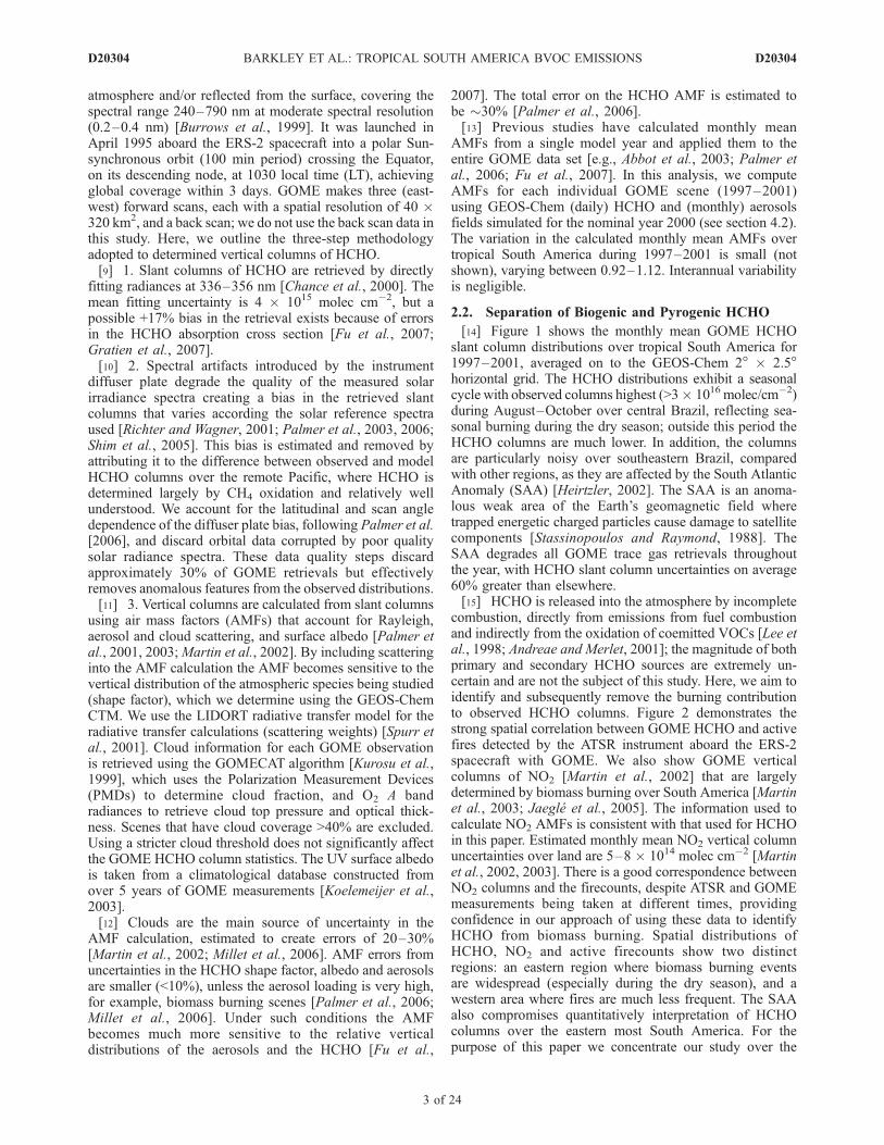
combustion, directly from emissions from fuel combustionand indirectly from the oxidation of coemitted VOCs [Lee etal., 1998; Andreae and Merlet, 2001]; the magnitude of bothprimary and secondary HCHO sources are extremely un-certain and are not the subject of this study. Here, we aim toidentify and subsequently remove the burning contributionto observed HCHO columns. Figure 2 demonstrates thestrong spatial correlation between GOME HCHO and activefires detected by the ATSR instrument aboard the ERS-2spacecraft with GOME. We also show GOME verticalcolumns of NO2 [Martin et al., 2002] that are largelydetermined by biomass burning over South America [Martinet al., 2003; Jaegle et al., 2005]. The information used tocalculate NO2 AMFs is consistent with that used for HCHOin this paper. Estimated monthly mean NO2 vertical columnuncertainties over land are 5–8 � 1014 molec cm�2 [Martinet al., 2002, 2003]. There is a good correspondence betweenNO2 columns and the firecounts, despite ATSR and GOMEmeasurements being taken at different times, providingconfidence in our approach of using these data to identifyHCHO from biomass burning. Spatial distributions ofHCHO, NO2 and active firecounts show two distinctregions: an eastern region where biomass burning eventsare widespread (especially during the dry season), and awestern area where fires are much less frequent. The SAAalso compromises quantitatively interpretation of HCHOcolumns over the eastern most South America. For thepurpose of this paper we concentrate our study over the


3 of 24

D20304

western region where we remove the residual burning signalfrom the observed HCHO columns.[16] Figure 3 shows the corresponding time series of the

monthly mean HCHO slant columns and NO2 verticalcolumns over the eastern region defined by Figure 2 wherethere is active burning. There is a strong temporal correla-tion (r = 0.8) as the amount of HCHO and NO2 in theatmosphere peaks about 1–2 months after the maximumfrequency in active fires (which typically occurs at thebeginning of August). Enhanced HCHO production fromelevated isoprene emissions during August–October (whentemperatures and light levels are highest) and release ofHCHO from smouldering fires will contribute to this slightphase lag [Yokelson et al., 1997]. Sampling and instrumen-tal issues associated with the firecount data, such asnighttime measurements and inclusion of nonvegetationfires [Mota et al., 2006], will also likely contribute to thisphase difference.[17] We adopt a two-step approach to ensure that

pyrogenic contributions to observed HCHO columns areremoved from subsequent analysis of GOME data. First,the ATSR firecount data are mapped on to the GEOS-Chemgrid (2� � 2.5�), and HCHO data falling in grid pointswhere there is active fire are excluded from subsequentanalysis. We recognize the shortcomings of the firecount

data [Mota et al., 2006] but they nevertheless providevaluable information on the location and frequency ofactive fires. Second, we use elevated NO2 columns as amarker of biomass burning to discard corresponding HCHOcolumns. We use the 1997–2001 monthly mean time seriesof NO2 columns (Figure 3) to determine a columnthreshold, above which indicates biomass burning. Withinthe burning season, defined here as August–November,both the HCHO and NO2 peak simultaneously. The meanNO2 during this season is 1.2 � 1015 molec cm�2, whilstin the rest of the year it is less than half this value.We employaNO2 threshold of 0.8� 1015molec cm�2, determined by thetime series. Outside the burning season the monthly meanNO2 columns rarely exceed this threshold level.

3. Modeling HCHO Columns Over TropicalSouth America

3.1. GEOS-Chem Chemistry Transport ModelFramework

[18] GEOS-Chem is a global 3-D chemistry transportmodel (v7.04), applied here to simulate O3-NOx-VOC-aerosol for the interpretation of HCHO columns from theGOME instrument. The model is forced with assimilatedmeteorological data from the Goddard Earth Observing

Figure 1. Monthly mean GOME HCHO slant columns (molec cm�2) over tropical South America forJanuary–December 1997–2001, averaged on the GEOS-Chem 2� � 2.5� grid. The GOME data are for1000–1200 local time (LT) and correspond to observations with cloud cover �40%. No measurementsare available for February, November, and December of 2001. HCHO column data southeast of the blackline are compromised by the South Atlantic Anomaly (section 2.2).


4 of 24

D20304

System (GEOS-4) of the NASA Global Modelling andAssimilation Office (GMAO) [Bey et al., 2001]. TheGEOS-4 data have a 6-hour temporal resolution (3-hourfor surface variables and mixing depths) and a 1� � 1.25�horizontal resolution. There are 55 hybrid eta levels thatextend from the surface to 0.01 hPa. The boundary layer upto 2 km is resolved by 5 layers with midpoints at 58, 249,615, 1197 and 1986 m for a column based at sea level. Weuse the model at 2� � 2.5� horizontal grid and with 30 etalevels, with levels above �50 hPa lumped together.

[19] The chemistry mechanism, based on work byHorowitz et al. [1998], has approximately 80 species and300 reactions, and includes modifications by Bey et al.[2001], Fiore et al. [2002], Martin et al. [2003] and Parket al. [2004]. It includes a detailed representation of oxida-tion pathways for five nonmethane hydrocarbons (ethane,propane, lumped >C3 alkanes, lumped >C2 alkenes andisoprene). Under low NOx conditions (<0.1 ppb), astypically found in tropical ecosystems away from regionsof burning [Jacob and Bakwin, 1992; Andreae et al.,

Figure 2. Monthly mean (left) GOME HCHO slant columns and (right) GOME NO2 vertical columnsaveraged on the GEOS-Chem 2� � 2.5� grid for August–October 1997. Active burning, detected by theATSR instrument, is shown by grey diamonds. The distinct fire spatial distributions allow tropical SouthAmerica to be split into an eastern region where biomass burning is very common, and a western regionwhere wild fires are less prominent (black boxes).


5 of 24

D20304

2002], the HCHO molar yields predicted by GEOS-Chemand the Master Chemical Mechanism (MCM v3.01) [Blosset al., 2005] after 1 day, are 0.95 and 1.6 respectively,comprising 66% and 68% of their ultimate HCHO yields[Palmer et al., 2006]. This provides confidence that we canrelate observed HCHO column variability to emissions ofisoprene under low NOx conditions. However, these modelHCHO yields from isoprene oxidation at low NOx concen-trations are considerably uncertain, reflecting current uncer-tainties in the chemistry. Production of HCHO from a- andb-pinenes and methylbutenol (MBO) are parameterizedusing MCM calculations [Palmer et al., 2006]. Previousstudies of HCHO columns over North America showed thatHCHO columns from monoterpenes and MBO were indis-tinguishable from noise in the column measurements[Palmer et al., 2006]. We assessed the contribution ofmonoterpenes and MBO to HCHO columns over tropicalSouth America by performing a sensitivity simulationwithout their HCHO production. Similarly, we find theiremissions contribute only a small fraction of the HCHOcolumn (not shown), comparable in magnitude to thespectral fitting uncertainty of GOME HCHO columns.

3.2. Emissions Inventories

[20] Biomass burning emissions, for 15 species includingHCHO, are from the Global Fire Emission Databaseversion 2 (GFEDv2) [Giglio et al., 2003, 2006; van derWerf et al., 2006]. The GFED inventory uses 1� � 1�monthly carbon emissions (g C m�2), determined usingsatellite firecount data and the CASA biogeochemicalmodel [Potter et al., 1993], that are scaled by tracerspecific emissions factors [Andreae and Merlet, 2001], asa function of vegetation type, to produce an estimate ofthat tracer’s biomass burning emissions (which are sub-sequently regridded to the GEOS-Chem grid). During1997–2001 GFED estimates of global emissions of HCHOare 1.55–2.81 Tg C, of which 0.13–0.35 Tg C originates

from the eastern and western regions over tropical SouthAmerica (Figure 2). Anthropogenic emissions are describedby Park et al. [2004].[21] Biogenic emissions of isoprene, monoterpenes and

methylbutenol (MBO) are based on the Model of Emis-sions of Gases and Aerosols from Nature (MEGAN)[Guenther et al., 2006]. Emissions of limonene, a BVOCwith a potentially large but unquantified HCHO time-dependent yield, are not considered in this study as theyonly comprise 2–10% of the total monoterpene speciesover the Amazon Basin [Kesselmeier et al., 2000, 2002b].[22] MEGAN contains significant improvements to the

base emission factors and driving algorithms in relation tothe GEIA inventory [Guenther et al., 1995]. Isopreneemissions E in MEGAN are parameterized as

E ¼ E0 � gT � gPAR � gLAI � gAge � gSM � r; ð1Þ

where E0 is the baseline emission factor for standardconditions (in mg of isoprene m�2 h�1), which is adjustedto the local environmental conditions by dimensionless‘‘activity’’ factors that correct for variations in leaftemperature gT (as a function both of the currenttemperature and the average over the last 15 days),photosynthetically active radiation (PAR) gPAR, leaf areaindex gLAI, leaf age gAge and soil moisture gSM. Each of theactivity factors are normalized to standard conditions (airtemperature = 303 K, PAR = 1500 mmol m�2 s�1, leaf areaindex = 5, soil moisture = 0.3 m3 m�3). The effect of soilmoisture gSM is not taken into account in the currentGEOS-Chem implementation of MEGAN. A recent studyhas shown that gSM is close to unity over tropical SouthAmerica throughout the year [Muller et al., 2008]. Isopreneproduction and losses within the vegetation canopy itself,represented by the normalized ratio r, are also notimplemented (i.e., r = 1).

Figure 3. Time series of the monthly mean gridded GOME HCHO slant columns (dotted light greyline) and GOME NO2 vertical columns (solid black line), over the eastern region during 1997–2001,calculated using only grid squares in which wild fires occur. The corresponding total number of ATSRfirecounts is shown by the dashed dark grey line. The NO2 threshold of 0.8 � 1015 molec cm�2 used toidentify biomass burning is shown as the solid horizontal black line. The beginning (August) and end(November) of the burning season is indicated by the solid vertical black lines.


6 of 24

D20304

[23] In standard GEOS-Chem simulations, the baselineMEGAN isoprene emission factors are regridded from 1� �1� to the GEOS-Chem horizontal resolutions and driven by3-hourly surface air temperatures (at 2 m height), and bydiffuse and direct PAR from GEOS-4. Variations in LAI arebased on monthly mean values for the year 2000, derivedfrom the Advanced Very High Resolution Radiometer(AVHRR) [Myneni et al., 1997].

4. Model Evaluation

[24] In this section, we evaluate the ability of MEGANand GEOS-Chem to reproduce observed isoprene andHCHO concentrations from aircraft [Kuhn et al., 2007],balloon [Helmig et al., 1998], and tower [Kesselmeier etal., 2002b; Trostdorf et al., 2004] platforms over tropicalSouth America (validation data are summarized in Table 2;measurement locations are shown in Figure 4). The readershould be aware that the balloon measurements of Helmiget al. [1998] have been used to construct the MEGANisoprene emission inventory over South America. Toprovide the reader with some idea of the uncertaintyassociated with regional modeling of isoprene emissionswe have included in this section four model runs that use

different versions of MEGAN and different temperaturefields to drive MEGAN.[25] 1. MEGAN v2004 uses base emission factors E0,

downloaded from the National Centre for AtmosphericResearch (NCAR) website in 2004 (referenced online asMEGANv1; http:/bai.acd.ucar.edu/Megan/index.shtml),driven by the air temperature 2 m above the surface, T(0).The v2004 map is based on 7 field studies conducted in theAmazon between 1979 and 2000 [Guenther et al., 2006].[26] 2. MEGAN v2004 T(1) is the same asMEGAN v2004

but is driven by temperature in the first model layer, T(1).Mature rainforest canopies can be as high at 40–50 m, whichis comparable with the thickness of the first GEOS-Chemmodel layer (�100 m). T(1) is on average 1.6 K lower thanT(0), and represent a 6-hour average instead of a 3-houraverage.[27] 3. MEGAN v2006 uses base emission factors

downloaded from NCAR in 2006 (referenced online asMEGANv2), driven by the surface air temperature. Thev2006 emission factors are based on the original v2004map, but include updates from (1) an additional 5 studiesconducted between 2000 and 2004 in Amazonia and theGuyanas, and (2) more recent vegetation distribution mapsthat indicate a high fraction of isoprene emitting species (e.g.,

Figure 4. Site locations of the in situ measurements (symbols) used to validate GEOS-Chem (section 4)and to construct the MEGAN bottom-up inventory [Guenther et al., 2006] (black orthogonal crosses).The solid black line represents the division between the east and west regions defined in Figure 2.

Table 2. Summary of the Validation Data Used to Assess GEOS-Chem

LocationRainforest

TypeSpeciesMeasured

SamplingPeriod

SamplingPlatforma Reference

�500 km west of Iquitos, Peru Primary Isoprene July 1996 Tethered Balloon Helmig et al. [1998]Tapajos National Forest, Brazil Primary Isoprene 2002 Tower (�59 m) Trostdorf et al. [2004]60 km NNW of Manaus, Brazil Mature Isoprene July 2001 Aircraft Kuhn et al. [2007]Tower A, Rebio Jaru, Rondonia, Brazil Primary HCHO May, Oct 1999 Tower (24–52 m) Kesselmeier et al. [2002b]IBAMA, Rebio Jaru, Rondonia, Brazil Secondary HCHO May, Oct 1999 Scaffold (8–10 m) Kesselmeier et al. [2002b]

aThe sampling heights for the towers and scaffold are shown in brackets.


7 of 24

D20304

bamboo, palm) in regions such as the Brazil/Peru border[Guenther et al., 2006].[28] 4. MEGAN v2006 T(1) uses the v2006 emission

factors, as described above, but driven with the temperatureof the first model layer, T(1).[29] Figure 5 shows in general v2006 isoprene emission

factors are larger than those from v2004, with the exceptionof Southeast Brazil. The largest differences occur over theBrazil-Peru border, along the east coast over Guyana,Suriname and French Guiana, and over a transect over Brazilwhich approximately follows the Rio Tapajos and RioJuruena rivers (reflecting observations madewithin the RebioJaru ecological reserve [see, e.g., Greenberg et al., 2004]).[30] For each individual data set we sampled the model at

the time and location of the data. For computationalexpediency, we ran the model at a reduced spatial resolutionof 4� � 5�. All individual model runs were spun up for atleast 2 months from initial conditions, based on previous(6 month) model runs, to let the tracer distributions stabilize.

4.1. Isoprene: Vertical Profiles and Seasonal Cycle

[31] Helmig et al. [1998] determined vertical profiles ofisoprene and four monoterpenes during 7–15 July 1996

over the Peruvian Amazon, approximately 500 km west ofIquitos, by collecting air samples onto solid adsorbentcartridge packages that were attached to a balloon andtether line. These experiments resulted in 10 verticalisoprene profiles between the surface (2 m) and up to1600 m height within a primary tropical forest site, ofaverage canopy height 20–30 m. Figure 6 shows a generalgood agreement between the isoprene in six selectedprofiles and simulations from the MEGANv2004 T(1)model; the other simulations show a significant positivebias. In contrast to the in situ measurements, which show arapid decay of isoprene at approximately 1500 m, themodels exhibit a much slower decline with altitude asconcentrations are well-mixed in the PBL. This disagree-ment either suggests that (1) isoprene is being consumedabove the PBL faster (at this location) than currentlysimulated or (2) more likely reflects the difference in thePBL heights of the in situ point measurements (<1500 m)and the relatively coarse model grid square (1500–2000 m).[32] Kuhn et al. [2007] employed an automated VOC

sampler onboard an EMB 1001B1 aircraft, to sample theabove-canopy atmosphere over the central Amazon basin

Figure 5. (top) The annual MEGAN isoprene emission factors (mg of isoprene m�2 h�1) normalized tostandard conditions, on 1� � 1� grid, downloaded from NCAR in (left) 2004 and (middle) 2006, and(right) their difference (v2006–v2004). (bottom) The corresponding GEOS-Chem HCHO verticalcolumns (molec cm�2) computed for August 2000, sampled at the same time and location of individualGOME observations with cloud cover �40%, averaged onto the GEOS-Chem 2� � 2.5� grid. Themaximum difference between the HCHO columns is 1.8 � 1016 molec cm�2.


8 of 24

D20304

during 5–17 July 2001. Figure 7 shows that the observa-tions and the models agree on the confinement of isopreneto the lowermost 1500 m of the atmosphere, though theobservations show a faster decline with altitude near thesurface than the model, reflecting errors in model chemis-try and transport. The best agreement to the observations isfound with MEGANv2004, particularly with the T(1)temperature correction, with average positive model biasof 1–2 ppb. The MEGANv2006 models significantlyoverestimate the observed isoprene concentrations.[33] Figure 8 shows the only (almost) complete observed

seasonal cycle of isoprene concentrations currently avail-able over the Amazon Basin at Tapajos National Forest,Brazil [Trostdorf et al., 2004]. The observations show astrong seasonal variation with high isoprene concentrations(3–5 ppbv) in both the wet and dry seasons, separated bylower concentrations (1 ppbv) during a wet to dry transi-tional period (June–July). The measurements also showthat isoprene concentrations are typically 30% higher in thedry season than the wet season, the reason for which isunresolved. Trostdorf et al. [2004] suggest it is linked withwater availability but it is also possible that changes invegetation phenology are responsible [Kesselmeier, 2004;Kuhn et al., 2004a]. Dry season isoprene concentrationincreases of 100% have been observed elsewhere in theAmazon [Kesselmeier et al., 2002b]. The models are

generally unable to reproduce this pronounced seasonalcycle, with model isoprene concentrations much higher thanobservations. MEGAN v2004 produces a much closer matchto the observations than MEGAN v2006, reproducing theobserved variability in the dry season but having a positivebias during the rest of the year. The MEGAN v2004 T(1)simulation fails to capture the dry season isoprene mixingratios but more accurately estimates the annual mean and hasan overall negative bias of 1%, compared with MEGANv2004 (27%), MEGAN v2006 (60%) and MEGAN v2006T(1) (41%) model runs. Model bias is defined here, andelsewhere in the paper, as

bias ¼ 1001

n

Xni¼1

Qmi � Qo

i

max Qmi ;Q

oið Þ ; ð2Þ

where Qim and Qi

o are the model and observed quantitiesrespectively [Balkanski et al., 1993]. On the basis of theseavailable observations the MEGAN v2004 T(1) simulationproduces the closest match to the observed isoprene mixingratios over central Amazonia.

4.2. HCHO: Season Cycle

[34] Here, we examine model and observed surfaceHCHO concentrations at two towers within the Rebio Jaruecological reserve, located 100 km north of Ji-Parana in the

Figure 6. Comparison of model isoprene profiles (ppb) with six of the in situ tethered balloonmeasurements, observed within the Peruvian Amazon (4.58�S, 77.4�W) during July 1996 [Helmig et al.,1998]. Observations are shown in black, alongside the respective MEGAN v2004 (green), MEGANv2004 T(1) (blue), MEGAN v2006 (red), and MEGAN v2006 T(1) (yellow) model simulations.


9 of 24

D20304

Figure 7. Comparison of model isoprene profiles (ppb) from the four MEGAN simulations (section 4)with aircraft observations over central Amazon (approximately 60 km NNW of Manaus, Brazil), duringJuly 2001 [Kuhn et al., 2007]. All aircraft flights took place during the morning (1000–1200 LT), with atypical flight pattern consisting of a continuous spiral upward from >50 m to >3000 m in altitude,followed by a stepwise spiral descent within the vicinity of the K34 tower (2.58�S, 60.20�W) located inthe Reserva Biologica do Cuieiras forest reservation.

Figure 8. Comparison of model isoprene mixing ratios, corresponding to 1000–1200 LT (sampleddaily), with in situ tower measurements (sampling height �60 m) made within the National Forest ofTapajos (3.0�S, 54.9�W), Brazil, during 2002 [Trostdorf et al., 2004]. The model simulations are:MEGAN v2004 (green), MEGAN v2004 T(1) (blue), MEGAN v2006 (red), and MEGAN v2006 T(1)(yellow) (section 4).


10 of 24

D20304

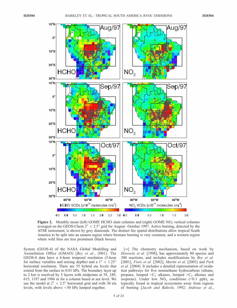
state of Rondonia, Brazil [Kesselmeier et al., 2002b].Measurements of HCHO concentrations were made duringthe ‘‘wet-to-dry’’ (April–May) and ‘‘dry-to-wet’’ (September–October) transition periods of 1999, as part of theLBA-EUSTACH-1 and LBA-EUSTACH-2 campaigns,respectively [Andreae et al., 2002], providing someinsight into the seasonal cycle. One tower (hereinafterknown as Tower A) was located within the Rebio Jaru naturereserve (10�0405500S, 61�5504800W), and the other tower waslocated at the Brazilian Environmental Protection AgencyInstituto Brasileiro de Meio Ambiente e Recursos Renova-veis (IBAMA) camp (10�0804300S, 61�5402700W). Tower Awas situated within primary rainforest and the IBAMA towerwas located at the edge of secondary forest; canopy heightswere 25–45m and 8–15m respectively. The sampling intakeheights for the HCHO observations used within this workwere 52 m (Tower A) and �10 m (IBAMA).[35] Figure 9 shows that the model and observed con-

centrations are generally higher by a factor of 2–3 in the‘‘dry-to-wet’’ period. The model generally has a positivebias in the ‘‘wet-to-dry’’ months (especially at the IBAMAtower), but shows reasonable agreement during the ‘‘dry-to-wet’’ months. MEGAN v2004 T(1) HCHO concentra-tions are the most consistent with observed values. We findthat MEGAN v2004 and MEGAN v2006 T(1) HCHOconcentrations are almost indistinguishable. ObservedHCHO concentrations show a strong diurnal cycle, withvalues peaking in late afternoon and decreasing close to zeroduring night, reflecting the diurnal cycle of isoprene emis-sion and its photochemical destruction, and uptake of HCHOby vegetation and soils [Jacob and Wofsy, 1988; Kuhn et al.,2002; Rottenberger et al., 2004]. Model HCHO concentra-tions have a similar diurnal cycle, but HCHO remainsrelatively high during nighttime. We attribute this to themodel nighttime boundary layer falling below the thicknessof the first model layer (�130 m). Above the boundary layer,nighttime isoprene concentrations are assumed to be com-parable to daytime values [Rasmussen and Khalil, 1988].This nighttime excess of isoprene can be converted toHCHO via reaction with O3 and the nitrate radical NO3.Simulated and observed isoprene mixing ratios at theIBAMA camp (not shown) exhibit the same characteristicsof the respective HCHO data sets.[36] Figure 10 shows that monthly mean GOME HCHO

vertical columns over western South America (defined inFigure 2) peak in the March (wet season) and August–September (dry season), with very low HCHO columns(close to values determined solely by CH4 oxidation)during a transition period in May. The low HCHO columnsobserved in May are suggestive of a dramatic reduction inHCHO production and are consistent with the low HCHOmixing ratios observed at the IBAMA and tower A sites(Figure 9). Dry season columns are typically 20% higherthan wet season columns. This seasonal cycle is consistentwith that of isoprene concentrations shown above inFigure 8. Owing to the fire-screening procedure, the annualand dry season mean HCHO columns over the westernzone are 23% and 66% lower than the corresponding meancolumns over the eastern region, respectively.[37] Model HCHO columns are generally higher than

observed values and do not reproduce the observed seasonalcycle, with columns gradually increasing during May–July

reaching a peak in the dry season. Table 3 shows that theannual mean model biases (exclusive of active burningregions) range from 35 to 56%, depending on the modelused, with the MEGAN v2004 T(1) simulation providingthe best fit to observed columns. The model bias is smallerwhen both east and west regions are considered together,although the spatial correlation with the GOME HCHOcolumns is worse. Two possible reasons for the positivemodel bias include (1) the MEGAN isoprene emissions aretoo high, and (2) physical processes (e.g., dry deposition,turbulent mixing) and also above and within-canopy chem-istry is inadequately represented in the model (section 6).In the latter case, the use of the newer (higher) v2006emission factors, will amplify this model shortcomingleading to a larger model bias (even if the emission factorsare considered to be more accurate). Compared with GEIA[Guenther et al., 1995], the isoprene emissions over thewestern region predicted by the MEGAN v2004 T(1) andv2006 T(1) simulations are, on average, 30% and 54%higher. However, tropical rainforest emissions in GEIA arebased on ambient isoprene concentration measurementsfrom only a single study [Zimmerman et al., 1988] andare therefore much more uncertain.[38] The MEGAN v2004 T(1) model generally provides

the closest match to observed concentrations of isopreneand HCHO, and will be used in subsequent model calcu-lations performed at an increased 2� � 2.5� horizontalresolution. The higher-resolution simulation was initializedby a 6-month spin up from July to December of 1999, andthen restarted to run through January to December of 2000.The HCHO shape factors and aerosol fields, used tocalculate the GOME AMFs (section 2.1), are taken fromthis simulation.

5. Isoprene Emissions Inferred From HCHOColumns

5.1. Methodology

[39] The method adopted to infer VOC emissions fromHCHO columns is based on mass balance and followsPalmer et al. [2003]. VOCs emitted into the column at arate Ei (atom C cm�2 s�1) are oxidized producing HCHOwith a per carbon yield Yi, with HCHO losses by oxidationand photolysis denoted by the first-order column-integratedloss rate constant kHCHO (s�1). Assuming steady stateconditions, and neglecting horizontal transport, the resultingHCHO column W, and its relation to parent VOC emissions,is given by

W ¼ 1

kHCHO

Xi

YiEi: ð3Þ

Horizontal transport spatially smears this local relationshipby an amount that depends on the wind speed, the rate ofproduction of HCHO from parent VOCs and the lifetime ofHCHO. VOCs with large emissions, high HCHO yieldsand short lifetimes will generally determine the variabilityof HCHO columns, with long-lived VOCs (e.g., CH4)largely determining background concentrations. Previousstudies over North America in summertime have shownthat isoprene, with a lifetime of approximately an hour anda HCHO yield of 0.3–0.4 C�1 depending on NOx


11 of 24

D20304

concentrations, have a spatial smearing length of <100 km[Palmer et al., 2003, 2006]. This length scale iscomparable with the horizontal dimensions of GOMEpixels (40 � 320 km2), suggesting that observed variabilityof GOME HCHO is determined largely by isopreneoxidation [Palmer et al., 2003, 2006; Millet et al., 2006].Other short-lived biogenic VOCs with similar HCHO

yields, such as a- and b-pinene, have a delayed productionof HCHO due to the acetone oxidation intermediate,leading to a smearing length of many 100s km.[40] Over the Amazon, model emissions of monoterpenes

and MBO are typically an order and 3 orders of magnitudeless than the emissions of isoprene, respectively. Figure 10shows that isoprene is the primary driver for variability of

Figure 9. Comparison of model HCHO mixing ratios with in situ tower measurements made within theRebio Jaru ecological reserve, Rondonia, Brazil, at the IBAMA camp (10�0804300S, 61�5402700W)(top three panels) and at the Tower A site (10�0405500S, 61�5504800W) (bottom three panels), over differentsampling periods during 1999 [Kesselmeier et al., 2002b]. Blue and red dots denote morning andafternoon observations, respectively. See section 4.2 for further details.


12 of 24

D20304

model HCHO columns over tropical South America awayfrom biomass burning, and is supported by our analysis ofobserved NO2, HCHO and firecount data (section 2.2).[41] To infer isoprene emissions from GOME HCHO

observations, we linearly regress model isoprene emissionsEMEGAN (atom C cm�2 s�1) and HCHO columns WGEOS

(molec cm�2) that have been sampled at the time andlocation of each GOME observation and averaged on themodel 2� � 2.5� grid,

WGEOS ¼ SEMEGAN þ B: ð4Þ

The slope S (s) represents the HCHO column producedfrom the emission of isoprene, and the intercept B representsthe HCHO background from the oxidation of longer-livedVOCs. The transfer function used to estimate isopreneemissions that are consistent with observed HCHO columnscan be inferred by transposing equation (4) and using modelvalues of S and B,

EGOME ¼ WGOME � B

S: ð5Þ

Table 3. Comparison of GEOS-Chem and GOME HCHO Vertical Columns for 2000 Over Tropical South Americaa

Month

Biasb (%) Correlation rb

v2004 v2004 T(1) v2006 v2006 T(1) CORR v2004 v2004 T(1) v2006 v2006 T(1) CORR

Jan 23.1 (23.3) 15.1 (14.1) 29.6 (35.4) 21.8 (26.6) 9.3 (9.9) 0.36 (0.50) 0.38 (0.53) 0.27 (0.48) 0.30 (0.50) 0.48 (0.77)Feb 29.7 (30.6) 20.5 (20.8) 35.1 (44.1) 26.6 (35.0) 10.9 (11.9) 0.41 (0.76) 0.41 (0.75) 0.32 (0.75) 0.33 (0.45) 0.45 (0.82)March 48.7 (46.8) 43.1 (39.6) 53.9 (55.6) 48.6 (49.5) 37.5 (33.9) 0.15 (0.41) 0.17 (0.44) 0.19 (0.38) 0.21 (0.26) 0.26 (0.60)April 59.3 (59.2) 55.1 (54.5) 62.0 (66.1) 57.8 (61.6) 45.6 (47.2) 0.40 (0.50) 0.40 (0.51) 0.40 (0.48) 0.42 (0.48) 0.48 (0.61)May 48.1 (53.5) 43.3 (49.3) 51.4 (60.3) 46.4 (56.2) 33.3 (40.5) 0.30 (0.29) 0.32 (0.33) 0.24 (0.25) 0.26 (0.42) 0.42 (0.50)June 60.3 (67.1) 56.5 (63.4) 64.3 (72.8) 60.8 (69.5) 50.0 (57.1) 0.43 (0.45) 0.43 (0.46) 0.41 (0.43) 0.42 (0.49) 0.49 (0.56)July 31.4 (34.3) 24.1 (26.1) 40.3 (46.0) 33.3 (38.2) 14.7 (15.3) 0.21 (0.30) 0.23 (0.32) 0.18 (0.27) 0.19 (0.32) 0.32 (0.46)Aug 39.0 (46.6) 29.0 (36.1) 51.0 (59.7) 42.5 (51.0) 14.2 (20.3) 0.55 (0.55) 0.57 (0.58) 0.51 (0.51) 0.52 (0.64) 0.64 (0.66)Sept 33.3 (39.3) 21.8 (27.2) 46.4 (53.9) 36.4 (43.6) 9.3 (13.7) 0.65 (0.67) 0.69 (0.71) 0.58 (0.61) 0.62 (0.79) 0.79 (0.85)Oct 48.5 (52.4) 38.0 (42.3) 56.0 (59.9) 50.2 (54.7) 23.1 (27.6) 0.61 (0.57) 0.65 (0.60) 0.59 (0.55) 0.60 (0.77) 0.77 (0.74)Nov 42.2 (48.8) 33.9 (40.4) 49.8 (59.6) 42.5 (52.4) 20.3 (26.8) 0.42 (0.56) 0.45 (0.59) 0.35 (0.51) 0.38 (0.56) 0.56 (0.72)Dec 44.0 (39.6) 37.3 (32.5) 52.6 (50.9) 46.3 (44.1) 22.6 (16.6) 0.18 (0.42) 0.19 (0.42) 0.18 (0.42) 0.19 (0.24) 0.24 (0.54)

Mean 42.3 (45.1) 34.8 (37.2) 49.4 (55.5) 42.8 (48.5) 24.3 (26.7) 0.39 (0.50) 0.41 (0.52) 0.35 (0.47) 0.37 (0.49) 0.49 (0.65)aTropical South America is defined as the western and eastern regions shown in Figure 2.bModel biases (equation (7)) and correlations are for the MEGAN v2004, MEGAN v2004 T(1), MEGAN v2006, and rc corrected (CORR) simulations

respectively (sections 4 and 5.2), relative to the HCHO vertical columns observed by GOME (calculated using AMFs from the corresponding model run).Values in parentheses are for the western region alone.

Figure 10. Monthly mean GEOS-Chem and GOME HCHO vertical columns (molec cm�2) overwestern South America (Figure 2) calculated using fire-free regions (section 2.2). The ±1-s standarddeviation are shown on the GOME mean (black). The v2004, v2004 T(1), v2006, and v2006 T(1) modelsimulations are shown by the purple, blue, dark green, and yellow lines, respectively. A sensitivity runwithout any isoprene emissions (OFF) is given by the light green line. The HCHO columns from the rccorrected simulation (CORR) (discussed in section 5) are shown in red.


13 of 24

D20304

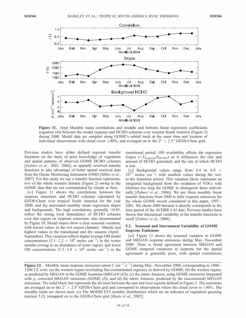
Previous studies have either defined regional transferfunctions on the basis of prior knowledge of vegetationand spatial patterns of observed GOME HCHO columns[Palmer et al., 2003, 2006], or spatially resolved transferfunctions to take advantage of better spatial resolved datafrom the Ozone Monitoring Instrument (OMI) [Millet et al.,2007]. For this study we use a transfer function representa-tive of the whole western domain (Figure 2) owing to theGOME data that are not contaminated by clouds or fires.[42] Figure 11 shows the correlations between the

isoprene emissions and HCHO columns calculated byGEOS-Chem over tropical South America for the year2000, and the associated monthly mean regression slopesand backgrounds. The high correlations, generally >0.85,reflect the strong local dependence of HCHO columnsover this region on isoprene emissions, also demonstratedby Figure 10. Model slopes show a clear seasonal variation,with lowest values in the wet season (January–March) andhighest values in the transitional and dry seasons (April–September). This variation reflects higher average OHmodelconcentrations (2.1–2.2 � 106 molec cm�3) in the wettermonths (owing to an abundance of water vapor), and lowerOH concentrations (1.3–1.8 � 106 molec cm�3) in the

transitional period. OH availability affects the regressionslopes (�YIsoprene/kHCHO) as it influences the rate andamount of HCHO generated, and the rate at which HCHOis lost.[43] Background values range from 4.4 to 6.9 �

1015 molec cm�2, with smallest values during the wet-to-dry transition period. This variation likely represents anintegrated background from the oxidation of VOCs withlifetimes too long for GOME to distinguish them individ-ually [Palmer et al., 2006]. We use these monthly lineartransfer functions from 2000 to infer isoprene emissions forthe whole GOME record considered in this paper, 1997–2001. We chose 2000 because it directly corresponds to thetime period of the AVHRR LAI data. Previous studies haveshown that interannual variability in the transfer functions issmall [Palmer et al., 2006].

5.2. Seasonal and Interannual Variability of GOMEIsoprene Emissions

[44] Figure 12 shows the seasonal variation in GOMEand MEGAN isoprene emissions during May–November2000. There is broad agreement between MEGAN andGOME temporal variations in isoprene but the spatialagreement is generally poor, with spatial correlations

Figure 11. (top) Monthly mean correlations and (middle and bottom) linear regression coefficients(equation (4)) between the model isoprene and HCHO columns over western South America (Figure 2)during 2000. Model data are sampled along GOME’s orbital track at the same time and location ofindividual observations with cloud cover �40%, and averaged on to the 2� � 2.5� GEOS-Chem grid.

Figure 12. Monthly mean isoprene emissions (atom C cm�2 s�1) during May–November 2000, corresponding to 1000–1200 LT, over: (a) the western region (excluding fire-contaminated regions), as derived by GOME; (b) the western region,as predicted by MEGAN at the GOME locations (MEGAN (G)); (c) the entire Amazon, using GOME emissions integratedwith rc corrected MEGAN emissions (GOME (I)); and (d) the entire Amazon, predicted by the (uncorrected) MEGANemissions. The solid black line represents the division between the east and west regions defined in Figure 2. The emissionsare averaged on to the 2� � 2.5� GEOS-Chem grid and correspond to observations where the cloud cover is �40%. Themonthly totals are shown inset. (e) The MODIS EVI monthly distributions which are an indicator of vegetation greening(section 5.2), remapped on to the GEOS-Chem grid [Huete et al., 2002].


14 of 24

D20304

typically <0.4. Spatial correlations between MEGAN andGOME, during August and September when emissionspeak, are much higher with values of 0.7 and 0.6, respec-tively. GOME and MEGAN agree on higher isopreneemissions during the dry season, determined in MEGAN

by the higher temperatures and light levels [Guenther et al.,1995]. MEGAN predicts much greater emissions thanGOME, over west Brazil during August–October. MEGANgenerally has a positive bias, with the bias larger in the dryseason than the wet season (Table 4).

Figure 12


15 of 24

D20304

[45] To develop a contiguous distribution of isopreneemissions over tropical South America for subsequent modelcalculations we combine MEGAN and GOME isopreneemissions, filling in undetermined grid squares (excludedbecause of biomass burning) using the model emissions. Wetake into account that MEGAN estimates isoprene emittedfrom the canopy foliage, whereas GOME infers the netisoprene flux emitted from above the forest canopy, i.e.,including above and within-canopy chemistry and physics,by approximating a canopy production and loss ratio, relativeto the model, rc,

r rc ¼EGOME � EMEGAN

EMEGAN

; ð6Þ

where EGOME and EMEGAN are the observed and modelisoprene emissions at each model grid square, respectively.The ratio rc reflects not only losses within the canopy butalso possible inadequately parameterized or poorly con-strained GEOS-Chem model processes (e.g., turbulentmixing, missing chemical sinks) within the PBL.[46] For each individual cloud-free GOME observation

we calculate a ‘‘corrected’’ MEGAN isoprene emissionsusing (EMEGAN)c = EMEGAN + (EMEGAN � rc). Values of rcrange �0.99 to 0.95. Monthly mean correction factors wereapplied to model grid points where rc was unable to becalculated, and additionally to those grid boxes falling in theeastern region (where burning is widespread and rc isconsidered only as a first approximation). Monthly meanrc values range from �0.25 to �0.44; the average monthlycorrection is �0.36. The correction factors are significantlygreater than current in-canopy loss estimates (�10%)[Guenther et al., 2006; Kuhn et al., 2007; Karl et al., 2007].[47] Figure 12 shows the contiguous isoprene distribution

determined by GOME and MEGAN for 2000. Note thatusing monthly mean rc to scale MEGAN isoprene emis-sions over the eastern region does not alter the spatialdistribution of emissions, reflected by spatial correlationsgiven in Table 4. We find that MEGAN isoprene emissionsare 33% higher than the emissions inferred from GOME(Table 4). During the dry season, the highest isopreneemitting areas are over central and western Amazon and

along the Brazilian borders with Peru and Bolivia. Figure 12also shows that variations in MEGAN and GOME isopreneemissions are consistent with variations in the EnhancedVegetation Index (EVI), an indicator of vegetation greening,determined from the MODIS sensor [Justice et al., 1998;Huete et al., 2002]. The average spatial correlation duringthe dry season, between the EVI and the GOME andMEGAN isoprene emissions are 0.57 and 0.64 respectively(over the combined eastern and western regions; seeTable 4). Recent studies have documented an average25% increase in EVI over the Amazon basin during thedry season when temperatures and level of sunlight aregenerally higher than the rest of the year [Huete et al., 2006;Saleska et al., 2007], suggesting that sunlight has moreinfluence on mature rainforest productivity than previouslythought. Deep rooting of mature plant species ensuresaccess to soil water throughout the year [Nepstad et al.,1994; da Rocha et al., 2004], so unless vegetation experi-ence severe drought stress isoprene emissions are unlikelyto be significantly affected [Pegoraro et al., 2006].[48] Figure 13 shows the contiguous GOME/MEGAN

isoprene emissions over 1997–2001. There is little year-to-year variation in the seasonal distribution of emissions overthis period, with emissions generally increasing from Mayand peaking in August and September, consistent with theseasonal variation in HCHO columns (Figure 1, section 2.2).The Amazon Basin (western Brazil) consistently has thelargest emissions, with emissions over the Guyannas, Peruand the northwestern countries generally lower. The highestannual isoprene emissions occur in El Nino years (1997/1998), owing to the associated warmer temperatures, inagreement with previous studies [e.g., Lathiere et al., 2006;Muller et al., 2008].[49] Figure 14 shows that including GOME isoprene

emissions in GEOS-CHEM improves the agreement betweenmodel and observed HCHO column, with the mean modelbias reduced from 35% to 24% and the spatial correlationincreased slightly from 0.41 to 0.46 (Table 3). If we consideronly the less noisy observed columns over the westernregion, the GOME isoprene emissions reduce the meanmodel bias from 36% to 25% and increase the spatial

Table 4. Summary of the GOME and MEGAN Isoprene Emissions for the Year 2000 Over Tropical South Americaa

Month

Monthly Totals (Tg C)

Bias (%) Correlation

EVI Correlationb

GOMEc MEGANd GOMEc MEGANd

Jan 19.2 (7.9) 24.9 (9.9) 19.3 (9.2) 0.71 (0.31) – – – –Feb 13.1 (3.0) 18.0 (4.2) 25.8 (21.4) 0.88 (0.60) 0.58 (0.45) 0.62 (0.57)March 11.4 (4.0) 15.7 (4.7) 27.5 (9.3) 0.70 (0.29) 0.46 (0.30) 0.60 (0.73)April 8.2 (2.5) 16.2 (4.5) 47.2 (31.6) 0.82 (0.46) 0.46 (0.24) 0.58 (0.57)May 12.4 (4.3) 21.9 (8.0) 37.8 (30.2) 0.72 (0.14) 0.43 (0.20) 0.53 (0.43)June 13.4 (4.5) 20.2 (6.8) 29.6 (19.8) 0.81 (0.33) 0.49 (0.11) 0.55 (0.38)July 12.6 (5.9) 19.1 (9.1) 28.4 (20.9) 0.72 (0.27) 0.45 (0.12) 0.68 (0.70)Aug 20.0 (8.2) 31.3 (13.0) 33.5 (30.3) 0.93 (0.70) 0.54 (0.36) 0.58 (0.50)Sept 23.0 (9.6) 33.6 (14.3) 27.8 (23.5) 0.90 (0.60) 0.58 (0.24) 0.63 (0.61)Oct 22.1 (6.1) 38.8 (11.0) 41.0 (37.3) 0.91 (0.49) 0.55 (0.14) 0.60 (0.48)Nov 11.6 (4.8) 19.3 (8.4) 36.1 (32.5) 0.78 (0.47) 0.59 (0.30) 0.74 (0.71)Dec 14.3 (3.6) 25.2 (6.2) 42.5 (36.2) 0.80 (0.23) 0.50 (�0.02) 0.66 (0.69)Mean 15.1 (5.4) 23.7 (8.3) 33.0 (25.2) 0.81 (0.41) 0.47 (0.20) 0.56 (0.53)

aTropical South America is defined as the western and eastern regions shown in Figure 2. Values in parentheses correspond to data over the westernregion alone (exclusive of fire-contaminated regions).

bThe correlation of the GOME and MEGAN isoprene emissions with the MODIS Enhanced Vegetation Index (EVI) (section 5.2).cThe GOME emissions are integrated with the rc corrected MEGAN values (section 5.2). Data over the western region correspond to top-down GOME

emissions only.dMEGAN emissions are taken from the v2004 T(1) simulation (section 4.2).


16 of 24

D20304

Figure

13.

Monthly

meanGOME-derived

isopreneem

issions(atom

Ccm

�2s�

1),

correspondingto

1000–1200LT,

integratedwithther c-correctedMEGAN

emissions(section5.2),over

tropical

South

AmericaduringMay

–Novem

ber

1997–2000.Theem

issionsareaveraged

onto

the2��

2.5�GEOS-Chem

gridandcorrespondto

observationswherethe

cloudcover

is�40%.Themonthly

totalsareshowninset.Thesolidblack

linerepresentsthedivisionbetweentheeastand

westregionsdefined

inFigure

2.


17 of 24

D20304

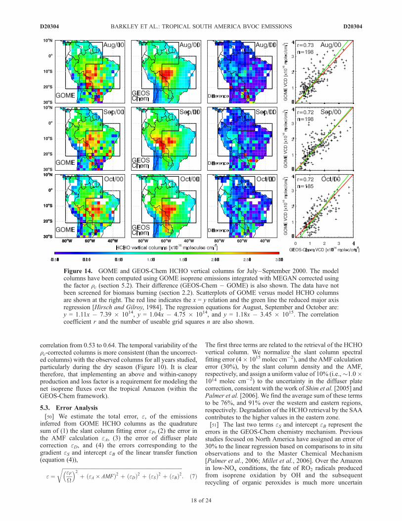
correlation from 0.53 to 0.64. The temporal variability of therc-corrected columns is more consistent (than the uncorrect-ed columns) with the observed columns for all years studied,particularly during the dry season (Figure 10). It is cleartherefore, that implementing an above and within-canopyproduction and loss factor is a requirement for modeling thenet isoprene fluxes over the tropical Amazon (within theGEOS-Chem framework).

5.3. Error Analysis

[50] We estimate the total error, e, of the emissionsinferred from GOME HCHO columns as the quadraturesum of (1) the slant column fitting error eF, (2) the error inthe AMF calculation eA, (3) the error of diffuser platecorrection eD, and (4) the errors corresponding to thegradient eS and intercept eB of the linear transfer function(equation (4)),

e ¼ffiffiffiffiffiffiffiffiffiffiffiffiffiffiffiffiffiffiffiffiffiffiffiffiffiffiffiffiffiffiffiffiffiffiffiffiffiffiffiffiffiffiffiffiffiffiffiffiffiffiffiffiffiffiffiffiffiffiffiffiffiffiffiffiffiffiffiffiffiffiffiffiffiffiffiffiffiffiffiffiffiffiffiffiffiffiffiffiffiffiffiffiffiffiffiffiffieFW

� �2

þ eA � AMFð Þ2 þ eDð Þ2 þ eSð Þ2 þ eBð Þ2r

: ð7Þ

The first three terms are related to the retrieval of the HCHOvertical column. We normalize the slant column spectralfitting error (4� 1015 molec cm�2), and the AMF calculationerror (30%), by the slant column density and the AMF,respectively, and assign a uniform value of 10% (i.e.,�1.0�1014 molec cm�2) to the uncertainty in the diffuser platecorrection, consistent with the work of Shim et al. [2005] andPalmer et al. [2006]. We find the average sum of these termsto be 76%, and 91% over the western and eastern regions,respectively. Degradation of the HCHO retrieval by the SAAcontributes to the higher values in the eastern zone.[51] The last two terms eS and intercept eB represent the

errors in the GEOS-Chem chemistry mechanism. Previousstudies focused on North America have assigned an error of30% to the linear regression based on comparisons to in situobservations and to the Master Chemical Mechanism[Palmer et al., 2006; Millet et al., 2006]. Over the Amazonin low-NOx conditions, the fate of RO2 radicals producedfrom isoprene oxidation by OH and the subsequentrecycling of organic peroxides is much more uncertain

Figure 14. GOME and GEOS-Chem HCHO vertical columns for July–September 2000. The modelcolumns have been computed using GOME isoprene emissions integrated with MEGAN corrected usingthe factor rc (section 5.2). Their difference (GEOS-Chem � GOME) is also shown. The data have notbeen screened for biomass burning (section 2.2). Scatterplots of GOME versus model HCHO columnsare shown at the right. The red line indicates the x = y relation and the green line the reduced major axisregression [Hirsch and Gilroy, 1984]. The regression equations for August, September and October are:y = 1.11x � 7.39 � 1014, y = 1.04x � 4.75 � 1014, and y = 1.18x � 3.45 � 1015. The correlationcoefficient r and the number of useable grid squares n are also shown.


18 of 24

D20304

[Palmer et al., 2003, 2006]. We therefore assign a higherestimate of 60% to the error in the regression gradient eS toreflect the incomplete knowledge of the more complexoxidation pathways, acknowledging that this estimate maybe conservative. We allocate an error of 15% to represent theuncertainty in the HCHO background, eB, from the oxidationof CH4 and other unparameterized or unknown VOCs.[52] Using these assigned values we calculate a total error

in the GOME isoprene emissions, derived over the westernregion, of about 98%. Errors associated with isopreneemissions inferred from GOME data over the easternregion, where we have used the average rc values (derivedfrom the western region), are much higher (>100%).Despite these top-down isoprene emissions being uncertainby at least a factor of 2 they are still comparable withcurrent bottom-up inventories whose emission estimatescan vary by at least a factor of 2 to 3 depending on thedriving variable data employed [Guenther et al., 2006].

5.4. What Controls Variations in Isoprene EmissionsOver the Amazon?

[53] Variations in isoprene emissions are predominatelydriven by fluctuations in temperature. Within MEGAN, thetemperature variability is parameterized by the activityfactor gT (equation (1)), which is defined as

gT ¼ Eopt � CT2 � exp CT1xð ÞCT2 � CT1 1� exp CT2xð Þð Þ ; ð8Þ

where x = (1/Topt � 1/T)/R with T the leaf temperature (K), Ris the gas constant, Eopt is the maximum value for gT, andTopt is the temperature at which gT = Eopt. Both CT1 = 76 ‘�1

MPa�1 mol and CT2 = 160 ‘�1 MPa�1 mol are empiricalcoefficients representing the activation and deactivationenergies of isoprene emissions, respectively [Guenther et al.,1999, 2006]. The functional form of equation (8) exponen-tially increases isoprene emissions with increasing leaftemperatures up to a maximum Topt, above which there is arapid fall-off reflecting a breakdown in leaf biochemistry[Singsaas and Sharkey, 2000]. Topt and Eopt are also afunction of the mean 24-hour average temperature (K) overthe past 15 days, T15 [Guenther et al., 1999],

Eopt ¼ 1:9 � expð0:125 T15 � 301:0ð ÞÞ ð9Þ

Topt ¼ 316:0þ 0:5 T15 � 301:0ð Þ: ð10Þ

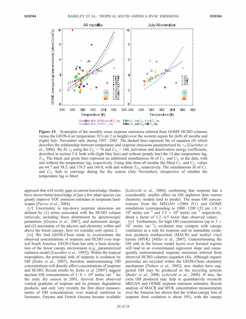
Figure 15 illustrates the dependence of the monthly meanisoprene emissions, inferred from GOME HCHO columnsover the western domain, as a function of the GEOS-4monthly mean T(1) air temperature used here as a proxyfor the current and average leaf temperatures over the past15 days, T and T15 respectively. The data show significantscatter and attempts to fit an exponential curve relating T(1)to GOME isoprene emissions were unsuccessful. Usingonly data from July–November of each year (nominal dryseason) we obtain a more significant relationship with airtemperature, although there remain several outliers. Weobtain a better fit to the data if we neglect T15. Including this15-day temperature lag yields a stronger exponentialdependence that appears more suited to the variation in theaverage emissions over all months. Fitted CT1 and CT2

values, using all data, are 64.7 and 58.5, and 176.5 and

166.0, with and without T15 respectively. The fittedactivation and deactivation energies are therefore smallerand larger than the standard values of Guenther et al. [2006],respectively. The simultaneous fit of CT1 and CT2 fails toconverge using the dry season data (July–November),irrespective of whether the temperature lag is fitted.[54] Monthly mean isoprene emissions outside of the dry

season vary considerably despite only small variations intemperature (�3 K), suggesting that during these monthsother factors are responsible for a large percentage of theobserved variability. The large variation in the observed wetseason emissions is also not explained with variations inPAR; although PAR is higher during the dry season its rangeof variability is typically the same during the wet and drymonths (�25–30 W m�2). Previous studies of in situ dataover the Amazon have concluded that water availability andchanges in leaf physiology and phenology also play a largerole in determining isoprene emission [Kuhn et al., 2004a,2004b] but their relative importance is a subject of continuingstudy. A recent study using MEGAN, driven at 0.5� � 0.5�resolution using ECMWF reanalyses, showed that includingprecipitation and soil moisture activity factors cannot rec-oncile model and observed isoprene fluxes over the Ama-zon during the wet season [Muller et al., 2008]. We find nosignificant correlation with the monthly mean GOMEisoprene emissions over western Amazonia with rainfall,PAR or soil moisture (not shown), suggesting that eitherGOME data are unsuitable (e.g., coarse horizontal resolu-tion, uncertainty) to study these local processes, or thatother, possibly nonenvironmental, forcings (e.g., leaf phys-iology) are driving observed variability.

6. Reconciling Bottom-Up and Top-DownIsoprene Emission Estimates

[55] There are notable differences between (1) MEGANbottom-up isoprene emissions and top-down isoprene emis-sions inferred from GOME, and (2) GEOS-Chem andobserved measurements of isoprene and HCHO. Here, weoffer some explanations that might help to reconcile thesediscrepancies.[56] Uncertainties in bottom-up isoprene emission models

generally arise from errors in emission factors, incorrect andincomplete parameterizations of activity factors, and uncer-tainties in the driving meteorological fields. As discussedabove, emission factors over South America (and in generaltropical ecosystems) are particularly uncertain, reflecting apaucity of in situ measurements with which to test anddevelop models over these region. The use of a single basalemission factor to represent isoprene emission over an entiregrowing season has already been shown to be inadequate forcertain tropical plant species [Kuhn et al., 2004a, 2004b].The large variation in the top-down isoprene emissionsoutside the dry season suggest it is determined by externalfactors other than temperature and light. Improved under-standing of plant physiological and phenological changes,and their possible incorporation into MEGAN, represents anavenue where more effort needs to be invested. Highbiodiversity of tropical ecosystems means that scaling upsparse, detailed point measurements is subject to largeerrors. A sustained programme of field measurements thatcatalogue emissions from tropical vegetation is the only


19 of 24

D20304

approach that will rectify gaps in current knowledge. Studieshave shown better knowledge of just a few plant species cangreatly improve VOC emission estimates in temperate land-scapes [Purves et al., 2004].[57] Uncertainty in top-down isoprene emissions are

defined by (1) errors associated with the HCHO columnretrievals, including those determined by spectroscopicparameters [Gratien et al., 2007], and instrument design,and (2) uncertainty of the physics and chemistry within andabove the forest canopy; here we consider only option 2.[58] We find GEOS-Chem tends to overestimate the

observed concentrations of isoprene and HCHO over trop-ical South America. GEOS-Chem has only a basic descrip-tion of the forest canopy environment (e.g., parameterizedradiation model [Guenther et al., 1995]). Within the tropicaltroposphere, the principal sink of isoprene is oxidation byOH [Kuhn et al., 2007]; therefore underestimating OHconcentrations will directly affect concentrations of isopreneand HCHO. Recent results by Kuhn et al. [2007] suggestdaytime OH concentrations of 3–8 � 106 molec cm�3 forthe early dry season in 2001, derived from observedvertical gradients of isoprene and its primary degradationproducts; and only very recently the first direct measure-ments of OH concentrations over tropical rainforest inSuriname, Guyana and French Guyana became available

[Lelieveld et al., 2008], confirming that isoprene has aconsiderably smaller effect on OH depletion than currentchemistry models tend to predict. The mean OH concen-trations from the MEGAN v2004 T(1) and GOMEsimulations (corresponding to 1000–1200 LT) are 1.8 �106 molec cm�3 and 2.5 � 106 molec cm�3 respectively,about a factor of 1.2–4.5 lower than observed values.[59] Furthermore, for high OH concentrations (up to 3 �

107 molec cm�3), oxidation may compete with canopyventilation as a sink for isoprene and its immediate oxida-tion products methacrolein (MACR) and methyl vinylketone (MVK) [Millet et al., 2007]. Underestimating theOH sink in the lowest model layers over forested regionswill lead to an overestimated regression slope and conse-quently underestimated isoprene emissions inferred fromobserved HCHO columns (equation (4)). Although organicperoxides are recycled within the GEOS-Chem chemistrymechanism [Palmer et al., 2003], new studies have sug-gested OH may be produced in the recycling process[Butler et al., 2008; Lelieveld et al., 2008]. If true, theextra OH produced may help to quantitatively reconcileMEGAN and GOME isoprene emission estimates. Recentanalysis of MACR and MVK concentration measurementsover the Amazon has shown that the within-canopy loss ofisoprene from oxidation is about 10%, with the canopy

Figure 15. Scatterplot of the monthly mean isoprene emissions inferred from GOME HCHO columnsversus the GEOS-4 air temperature T(1) (at 2 m height) over the western region for (left) all months and(right) July–November only during 1997–2001. The dashed lines represent fits of equation (8) whichdescribes the relationship between temperature and isoprene emissions parameterized by gT [Guenther etal., 2006]. We fit gT using the CT1 = 76 and CT2 = 160, activation and deactivation energy coefficients,described in section 5.4, both with (light blue line) and without (purple line) the 15-day temperature lag,T15. The black and green lines represent an additional simultaneous fit of CT1 and CT2 to the data, withand without the temperature lag, respectively. Using data from all months the fitted CT1 and CT2 valuesare 64.7 and 58.5, and 176.5 and 166.0, with and without T15, respectively. The simultaneous fit of CT1

and CT2 fails to converge during the dry season (July–November), irrespective of whether thetemperature lag is fitted.


20 of 24

D20304

ventilation rate much faster than the oxidation loss rate[Kuhn et al., 2007; Karl et al., 2007].[60] Observed vertical gradients of isoprene within forests

show very low near-surface isoprene concentrations [Kuhnet al., 2002], suggesting isoprene uptake at the forest floor.Field and laboratory studies indicate a biological sink ofisoprene sink exists within forest soils [Cleveland andYavitt, 1997, 1998], the magnitude and extent of whichremains unknown within tropical ecosystems. The magni-tude of a forest soil sink would also be susceptible toenvironmental forcings, such as drought stress [Pegoraroet al., 2006].[61] The direct exchange of HCHO between the atmo-

sphere and tropical vegetation is also poorly quantified,though in normal and high ambient aldehyde concentra-tions trees are most likely to act as sinks [Kondo et al.,1998]. Branch enclosure measurements at the Rebio Jaruecological reserve, demonstrated aldehyde uptake canoccur via leaf stomata and deposition to the leaf cuticles[Rottenberger et al., 2004]. Whilst the branch enclosuremeasurements also showed direct aldehyde emissions (atlow ambient concentrations), deposition of HCHO wasdominant in both wet and dry seasons, suggesting thattropical forests act as a direct sink for HCHO. It is likelythat the magnitude of both these sinks, however, may besmall in comparison to isoprene and HCHO losses throughoxidation and photolysis.[62] Our simple analysis of net canopy losses of isoprene

inferred from GOME, parameterized by the downscalingfactor rc applied to MEGAN (section 5.2), ranges from 25–44%, is much larger than estimates inferred from in situmeasurements [Kuhn et al., 2007; Karl et al., 2007], whichmay reflect uncertainties in the inference of top-downemissions and the inability of GEOS-Chem to representin-canopy processes.

7. Summary

[63] We have used a 6-year (1997–2001) data set ofHCHO columns from the Global Ozone MonitoringExperiment satellite instrument, in conjunction with theMEGAN bottom-up isoprene inventory and the GEOS-ChemCTM, to determine top-down isoprene emission estimatesover tropical South America. Bottom-up isoprene emissioninventories are particularly poorly quantified over tropicalecosystems, reflecting a sparsity of in situ data, high biodi-versity and inaccessibility. Space-borne measurements canhelp overcome many of these shortcomings.[64] Inferring isoprene emissions from HCHO columns

over tropical South America is significantly compromisedby (1) noise introduced to observed column over southeastSouth America from the SAA and (2) the source of HCHOfrom biomass burning. Both of these effects are mostpronounced over the eastern parts of the Amazon. For thisreason, we focus our study over the western region of SouthAmerica and extrapolate findings to the eastern regions. Weidentify and remove measurements compromised by activeburning that have been identified using ATSR firecountsand coincident GOME NO2 columns.[65] In the low NOx environment found over tropical

ecosystems, we find that isoprene largely determines theobserved variability in HCHO columns, with emissions of

a- and b-pinenes contributing only to the uniform back-ground, reflecting the production of the relatively long-lived acetone intermediate. Four different configurations ofthe GEOS-Chem/MEGAN models have been comparedwith in situ and aircraft isoprene and HCHO concentrationmeasurements over the Amazon. In general, model concen-trations have a positive bias that may reflect missing in-canopy chemistry. Uptake of isoprene by forest soils anddirect exchange of HCHO with vegetation are also possiblesink mechanisms that may be underestimated. Of the fourmodel configurations, it was determined that MEGANv2004 emission factors, driven by the temperature of thefirst GEOS-Chem model layer, produced the closest matchto the in situ measurements. This model, MEGAN v2004T(1), was subsequently used to determine the transferfunction that infers isoprene emissions from observedHCHO columns.[66] The resulting seasonal and year-to-year variations in

the isoprene emissions inferred from GOME show that thehighest-emitting region is consistently the Amazon basinwithin western Brazil. The emissions peak during the dryseason (August–November) and lower in the wet season. Inthe dry season, inferred emissions are consistent with thetemperature dependence predicted by MEGAN. Outside thedry season, other factors appear to also play a large role indetermining observed variability, however, we have notbeen able to identify a significant correlation with likelyfactors such as precipitation or soil moisture.[67] In general, GOME isoprene emissions are lower

than those predicted by MEGAN, reflecting partly thatGOME estimates represent net ecosystem fluxes whileMEGAN predicts leaf-level canopy emissions. Crudelyaccounting for net above and within-canopy losses, requiresMEGAN v2004 T(1) isoprene emissions to be reduced by33%. Differences between GOME and MEGAN can alsobe attributed to errors in the HCHO column retrieval and toerrors associated with the chemistry mechanism that deter-mines the transfer function. We calculate the total errorassociated with GOME isoprene emissions to be of order100%.[68] Future work will focus on using HCHO column

data from newer space-borne sensors that have 40 timesbetter spatial resolution and daily coverage, for example,OMI aboard NASA’s Aura satellite and GOME-2 aboardthe European MetOp platform. Using these sensors will(1) increase the number of cloud-free scenes that will improvethe signal-to-noise of averaged quantities; (2) improve thedifferentiation between biogenic and pyrogenic sources ofHCHO; and (3) broaden the process studies that can beachieved. A greater number of observations permits betterspatially resolved transfer functions [e.g., Millet et al.,2007]. However, as isoprene takes approximately an hourto produce (1 � 1/e) of its ultimate HCHO yield, itsaverage smearing length is about 100 km [Palmer et al.,2003]. Therefore, despite the higher resolution of newsensors 100 km may represent the spatial limit for inferringtop-down isoprene emissions estimates using the linearregression approach, beyond which a more formal inver-sion scheme would be required [Palmer et al., 2007].

[69] Acknowledgments. This work was supported by the NationalEnvironment Research Council (NERC research grant NE/D001471). The


21 of 24

D20304

authors would like to thank Tzung-May Fu, Dylan Millet, and RobertYantosca for useful help and advice. The GEOS-Chem model is managed atHarvard University with support from the NASA Atmospheric ChemistryModelling and Analysis Program. The authors would also like to thankKamel Didan and Alfredo Huete for providing the EVI data and the ESAportal for providing the ATSR firecounts.

ReferencesAbbot, D. S., P. I. Palmer, R. V. Martin, K. V. Chance, D. J. Jacob, andA. Guenther (2003), Seasonal and interannual variability of NorthAmerican isoprene emissions as determined by formaldehyde columnmeasurements from space, Geophys. Res. Lett., 30(17), 1886,doi:10.1029/2003GL017336.

Andreae, M. O., and P. J. Crutzen (1997), Atmospheric aerosols: Biogeo-chemical sources and role in atmospheric chemistry, Science, 276,1052–1058, doi:10.1126/science.276.5315.1052.

Andreae, M. O., and P. Merlet (2001), Emission of trace gases and aerosolsfrom biomass burning, Global Biogeochem. Cycles, 15(4), 955–966,doi:10.1029/2000GB001382.

Andreae, M. O., et al. (2002), Biogeochemical cycling of carbon, water,energy, trace gases, and aerosols in Amazonia: The LBA-EUSTACH ex-periments, J. Geophys. Res., 107(D20), 8066, doi:10.1029/2001JD000524.

Balkanski, Y. J., D. J. Jacob, G. M. Gardiner, W. C. Graustein, andK. K. Turekian (1993), Transport and residence times of troposphericaerosol inferred from a gloal three-dimensional simulation of 210Pb,J. Geophys. Res., 98(D11), 20,573–20,586, doi:10.1029/93JD02456.

Bey, I., et al. (2001), Global modeling of tropospheric chemistry withassimilated meteorology: Model description and evaluation, J. Geophys.Res., 106(D19), 23,073–23,096, doi:10.1029/2001JD000807.

Bloss, C., et al. (2005), Development of a detailed chemical mechanism(MCMv3.1) for the atmospheric oxidation of aromatic hydrocarbons,Atmos. Chem. Phys., 5, 641–664.

Burrows, J. P., et al. (1999), The Global Ozone Monitoring Experiment(GOME): Mission concept and first scientific results, J. Atmos. Sci., 56,151–175.

Butler, T. M., D. Taraborrelli, C. Bruhl, H. Fischer, H. Harder, M. Martinez,J. Williams, M. G. Lawrence, and J. Lelieveld (2008), Improved simula-tion of isoprene oxidation chemistry with the ECHAM5/MESSy chem-istry-climate model: Lessons from the GABRIEL airborne fieldcampaign, Atmos. Chem. Phys., 8, 4529–4546.

Chance, K., P. I. Palmer, R. J. D. Spurr, R. V. Martin, T. P. Kurosu, andD. J. Jacob (2000), Satellite observations of formaldehyde over NorthAmerica from GOME, Geophys. Res. Lett., 27(21), 3461 – 3464,doi:10.1029/2000GL011857.

Claeys, M., et al. (2004), Formation of secondary organic aerosols throughphotooxidation of isoprene, Science, 303, 1173–1176, doi:10.1126/science.1092805.

Cleveland, C. C., and J. B. Yavitt (1997), Consumption of atmosphericisoprene in soil, Geophys. Res. Lett., 24(19), 2379–2382, doi:10.1029/97GL02451.

Cleveland, C. C., and J. B. Yavitt (1998), Microbial consumption of atmo-spheric isoprene in a temperate forest soil, Appl. Environ. Microbiol.,64(1), 172–177.

da Rocha, H. R., M. L. Goulden, S. D. Miller, M. C. Menton, L. D. V. O.Pinto, H. C. de Freitas, and A. M. S. Figueira (2004), Seasonality ofwater and heat fluxes over a tropical forest in eastern Amazonia, Ecol.Appl., 14(4), supplement, S22–S32.

Davis, K. J., D. H. Lenschow, and P. R. Zimmerman (1994), Biogenicnonmethane hydrocarbon emissions estimated from tethered balloonobservations, J. Geophys. Res., 99(D12), 25,587–25,598, doi:10.1029/94JD02009.

Fiore, A. M., D. J. Jacob, I. Bey, R. M. Yantosca, B. D. Field, and J. G.Wilkinson (2002), Background ozone over the United States in summer:Origin and contribution to pollution episodes, J. Geophys. Res.,107(D15), 4275, doi:10.1029/2001JD000982.

Fu, T.-M., D. J. Jacob, P. I. Palmer, K. Chance, Y. X. Wang, B. Barletta,D. R. Blake, J. C. Stanton, and M. J. Pilling (2007), Space-based for-maldehyde measurements as constraints on volatile organic compoundemissions in east and south Asia and implications for ozone, J. Geophys.Res., 112, D06312, doi:10.1029/2006JD007853.

Giglio, L., J. Descloitres, C. O. Justice, and Y. J. Kaufman (2003), Anenhanced contextual fire detection algorithm for MODIS, Remote Sens.Environ., 87(2–3), 273–282.

Giglio, L., G. R. van der Werf, J. T. Randerson, G. J. Collatz, andP. Kasibhatla (2006), Global estimation of burned area using MODISactive fire observations, Atmos. Chem. Phys., 6, 957–974.

Gratien, A., B. Picquet-Varrault, J. Orphal, E. Perraudin, J.-F. Doussin, andJ.-M. Flaud (2007), Laboratory intercomparison of the formaldehydeabsorption cross sections in the infrared (1660–1820 cm�1) and ultra-

violet (300–360 nm) spectral regions, J. Geophys. Res., 112, D05305,doi:10.1029/2006JD007201.

Greenberg, J. P., A. Guenther, G. Petron, C. Wiedinmeyer, O. Vega, L. V.Gatti, J. Tota, and G. Fisch (2004), Biogenic VOC emissions fromforested Amazonian landscapes, Global Change Biol., 10, 651–662,doi:10.1111/j.1529-8817.2003.00758.x.

Guenther, A., et al. (1995), A global model of natural volatile organiccompound emissions, J. Geophys. Res., 100(D5), 8873 – 8892,doi:10.1029/94JD02950.

Guenther, A., B. Baugh, G. Brasseur, J. Greenberg, P. Harley, L. Klinger,D. Serca, and L. Vierling (1999), Isoprene emission estimates and uncer-tainties for the Central African EXPRESSO study domain, J. Geophys.Res., 104(D23), 30,625–30,639.

Guenther, A., T. Karl, P. Harley, C. Wiedinmyer, P. I. Palmer, and C. Geron(2006), Estimates of global terrestrial isoprene emissions using MEGAN(Model of Emissions of Gases and Aerosols from Nature), Atmos. Chem.Phys., 6, 3181–3210.

Heirtzler, J. R. (2002), The future of the South Atlantic anomaly andimplications for radiation damage in space, J. Atmos. Sol. Terr. Phys.,64(16), 1701–1708.

Helmig, D., et al. (1998), Vertical profiling and determination of landscapefluxes of biogenic non-methane hydrocarbons within the planetaryboundary layer in the Peruvian Amazon, J. Geophys. Res., 103(D19),25,519–25,532, doi:10.1029/98JD01023.

Henze, D. K., and J. H. Seinfeld (2006), Global secondary organic aerosolfrom isoprene oxidation, Geophys. Res. Lett., 33, L09812, doi:10.1029/2006GL025976.

Hirsch, R. M., and E. J. Gilroy (1984), Methods of fitting a straight line todata: Examples in water resources, Water Resour. Bull., 20, 705–711.

Horowitz, L. W., J. Liang, G. M. Gardner, and D. J. Jacob (1998), Export ofreactive nitrogen from North America during summertime: Sensitivity tohydrocarbon chemistry, J. Geophys. Res., 103(D11), 13,451–13,476,doi:10.1029/97JD03142.

Huete, A., K. Didan, T. Miura, E. P. Rodriguez, X. Gao, and L. G. Ferreira(2002), Overview of the radiometric and biophysical performance of theMODIS vegetation indices, Remote Sens. Environ., 83(1–2), 195–213.

Huete, A. R., K. Didan, Y. E. Shimabukuro, P. Ratana, S. R. Saleska,L. R. Hutyra, W. Yang, R. R. Nemani, and R. Myneni (2006), Amazonrainforests green-up with sunlight in dry season, Geophys. Res. Lett., 33,L06405, doi:10.1029/2005GL025583.

Jacob, D. J., and P. S. Bakwin (1992), Cycling of NOx in tropical forestcanopies, in Microbial Production and Consumption of GreenhouseGases, edited by W. B. Whitman, pp. 237–253, Am. Soc. of Microbiol.,Washington D. C.

Jacob, D. J., and S. C. Wofsy (1988), Photochemistry of biogenic emissionsover the Amazon Forest, J. Geophys. Res., 93(D2), 1477 – 1486,doi:10.1029/88JD01582.

Jaegle, L., L. Steinberger, R. V. Martin, and K. Chance (2005), Globalpartitioning of NOx sources using satellite observations: Relative rolesof fossil fuel combustion, biomass burning and soil emissions, FaradayDiscuss., 130, 407–423, doi:10.1039/b502128f.

Justice, C. O., et al. (1998), The Moderate Resolution Imaging Spectro-radiometer (MODIS): Land remote sensing for global change research,IEEE Trans. Geosci. Remote Sens., 36, 1228–1249.

Karl, T., A. Guenther, R. J. Yokelson, J. Greenberg, M. Potosnak,D. R. Blake, and P. Artaxo (2007), The tropical forest and fire emissionsexperiment: Emission, chemistry, and transport of biogenic volatileorganic compounds in the lower atmosphere over Amazonia, J. Geophys.Res., 112, D18302, doi:10.1029/2007JD008539.

Kesselmeier, J. (2004), Interactive comment on ‘‘Seasonal cycles ofisoprene concentrations in the Amazonian rainforest’’ by C. R. Trostdorfet al., Atmos. Chem. Phys. Discuss., 4, S528–S530.

Kesselmeier, J., et al. (2000), Atmospheric volatile organic compounds(VOC) at a remote tropical forest site in central Amazonia, Atmos.Environ., 34(24), 4063–4072.

Kesselmeier, J., et al. (2002a), Volatile organic compound emissions inrelation to plant carbon fixation and the terrestrial carbon budget, GlobalBiogeochem. Cycles, 16(4), 1126, doi:10.1029/2001GB001813.

Kesselmeier, J., et al. (2002b), Concentrations and species composition ofatmospheric volatile organic compounds (VOCs) as observed during thewet and dry season in Rondonia (Amazonia), J. Geophys. Res.,107(D20), 8053, doi:10.1029/2000JD000267.

Koelemeijer, R. B. A., J. F. de Haan, and P. Stammes (2003), A database ofspectral surface reflectivity of the Earth in the range 335–772 nm derivedfrom 5.5 years of GOME observations, J. Geophys. Res., 108(D2), 4070,doi:10.1029/2002JD002429.

Kondo, T., K. Hasegawa, R. Uchida, and M. Onishi (1998), Absorption ofatmospheric C2-C5 aldehydes by various tree species and their toleranceto C2-C5 aldehydes, Sci. Total Environ., 224, 121–132.


22 of 24

D20304

Kuhn, U., et al. (2002), Isoprene and monoterpene emissions of Amazoniantree species during the wet season: Direct and indirect investigations oncontrolling environmental functions, J. Geophys. Res., 107(D20), 8071,doi:10.1029/2001JD000978.

Kuhn, U., S. Rottenberger, T. Biesenthal, A. Wolf, G. Schebeske, P. Ciccioli,and J. Kesselmeier (2004a), Strong correlation between isoprene emissionand gross photosynthetic capacity during leaf phenology of the tropicaltree species Hymenaea courbaril with fundamental changes in volatileorganic compounds emission composition during early leaf development,Plant Cell Environ., 27, 1469–1485.

Kuhn, U., et al. (2004b), Seasonal differences in isoprene and light-dependent monoterpene emission by Amazonian tree species, GlobalChange Biol., 10, 663–682, doi:10.1111/j.1529-8817.2003.00771.x.

Kuhn, U., et al. (2007), Isoprene and monoterpene fluxes from centralAmazonian rainforest inferred from tower-based and airborne measure-ments, and implications on the atmospheric chemistry and the local car-bon budget, Atmos. Chem. Phys., 7, 2855–2879.

Kurosu, T. P., K. Chance, andR. J. D. Spurr (1999), CRAG—CloudRetrievalAlgorithm for ESA’s Global Ozone Monitoring Experiment, paperpresented at European Symposium on Atmospheric MeasurementsFrom Space, Eur. Space Agency, Noordwijk, Netherlands.

Lathiere, J., D. A. Hauglustaine, A. Friend, N. De Noblet-Ducoudre,N. Viovy, and G. Folberth (2006), Impact of climate variability and landuse changes on global biogenic volatile organic compound emissions,Atmos. Chem. Phys., 6, 2129–2146.

Lee, M., B. G. Heikes, and D. J. Jacob (1998), Enhancements of hydro-peroxides and formaldehyde in biomass burning impacted air and theireffect on atmospheric oxidant cycles, J. Geophys. Res., 103(D11),13,201–13,212, doi:10.1029/98JD00578.

Lelieveld, J., et al. (2008), Atmospheric oxidation capacity sustained by atropical forest, Nature, 452, 737–740, doi:10.1038/nature06870.

Liebmann, B., and J. A. Marengo (2001), Interannual Variability of therainy season and rainfall in the Brazilian Amazon Basin, J. Clim., 14,4308–4318.

Martin, R. V., et al. (2002), An improved retrieval of tropospheric nitrogendioxide from GOME, J. Geophys. Res., 107(D20), 4437, doi:10.1029/2001JD001027.

Martin, R. V., D. J. Jacob, K. Chance, T. P. Kurosu, P. I. Palmer, andM. J. Evans (2003), Global inventory of nitrogen oxide emissions con-strained by space-based observations of NO2 columns, J. Geophys. Res.,108(D17), 4537, doi:10.1029/2003JD003453.

Millet, D. B., et al. (2006), Formaldehyde distribution over North America:Implications for satellite retrievals of formaldehyde columns and isopreneemission, J. Geophys. Res., 111, D24S02, doi:10.1029/2005JD006853.

Millet, D. B., D. J. Jacob, K. Folkert Boersma, T.-M. Fu, T. P. Kurosu,K. Chance, C. L. Heald, and A. Guenther (2007), Spatial distributionof isoprene emissions from North America dervied from formaldehydecolumn measurements by the OMI satellite sensor, J. Geophys. Res.,113, D02307, doi:10.1029/2007JD008950.

Monson, R. K., and E. A. Holland (2001), Bisopheric trace gas fluxes andtheir control over tropospheric chemsitry, Annu. Rev. Ecol. Syst., 32,547–576.

Mota, B. W., J. M. C. Pereira, D. Oom, M. J. P. Vasconcelos, and M. Schultz(2006), Screening the ESA ATSR-2 World Fire Atlas (1997–2002),Atmos. Chem. Phys., 6, 1409–1424.

Muller, J.-F., et al. (2008), Global isoprene emissions estimated usingMEGAN, ECMWF analyses and a detailed canopy environment model,Atmos. Chem. Phys., 8, 1329–1341.

Myneni, R. B., R. R. Nemani, and S. W. Running (1997), Estimation ofglobal leaf area index and absorbed PAR using radiative transfer models,IEEE Trans. Geosci. Remote Sens., 35, 1380–1393.

Nepstad, D. C., C. R. de Carvalho, E. A. Davidson, P. Jipp, P. Lefebvre,G. H. Negreiros, E. D. da Silva, S. T. T. Stone, and S. Vieira (1994),The role of deep roots in the hydrological and carbon cycles of Amazonianforests and pastures, Nature, 372, 666–669, doi:10.1038/372666a0.

Palmer, P. I., et al. (2001), Air mass factor formulation for spectroscopicmeasurements from satellites: Application to formaldehyde retrievalsfrom the Global Ozone Monitoring Experiment, J. Geophys. Res.,106(D13), 14,539–14,550, doi:10.1029/2000JD900772.

Palmer, P. I., D. J. Jacob, A. M. Fiore, R. V. Martin, K. Chance, andT. P. Kurosu (2003), Mapping isoprene emissions over North Americausing formaldehyde column observations from space, J. Geophys. Res.,108(D6), 4180, doi:10.1029/2002JD002153.

Palmer, P. I., et al. (2006), Quantifying the seasonal and interannual varia-bility of North American isoprene emissions using satellite observationsof formaldehyde column, J. Geophys. Res., 111, D12315, doi:10.1029/2005JD006689.

Palmer, P. I., M. P. Barkley, T. P. Kurosu, A. C. Lewis, J. E. Saxton,K. Chance, and L. V. Gatti (2007), Interpreting satellite column observa-

tions of formaldehyde over tropical South America, Philos. Trans. R. Soc.,Ser. A, 365, 1741–1751.

Park, R. J., D. J. Jacob, B. D. Field, R. M. Yantosca, and M. Chin(2004), Natural and transboundary pollution influences on sulfate-nitrate-ammonium aerosols in the United States: Implications for policy,J. Geophys. Res., 109, D15204, doi:10.1029/2003JD004473.

Pegoraro, E., A. Rey, L. Abrell, J. Haren, and G. Lin (2006), Drought effecton isoprene production and consumption in Biosphere 2 tropical rain-forest, Global Change Biol., 12, 456–469, doi:10.1111/j.1365-2486.2006.01112.x.

Poisson, N., M. Kanakidou, and P. J. Crutzen (2000), Impact of non-methane hydrocarbons on tropospheric chemsitry and the oxidizingpower of the global troposphere: 3-dimensional modelling results,J. Atmos. Chem., 36, 157–230, doi:10.1023/A:1006300616544.

Potter, C. S., J. T. Randerson, C. B. Field, P. A. Matson, P. M. Vitousek,H. A. Mooney, and S. A. Klooster (1993), Terrestrial ecosystem pro-duction: A process model based on global satellite and surface data,Global Biogeochem. Cycles, 7(4), 811–841, doi:10.1029/93GB02725.

Potter, C. S., S. E. Alexander, J. C. Coughlan, and S. A. Klooster (2001),Modeling biogenic emissions of isoprene: exploration of model drivers,climate control algorithms, and use of global satellite observations,Atmos. Environ., 35(35), 6151–6165.

Purves, D. W., J. P. Caspersen, P. R. Moorcroft, G. C. Hurt, and S. W. Pacala(2004), Human-induced changes in US biogenic volatile organic com-pound emissions: evidence from long-term forest inventory data, GlobalChange Biol., 10, 1737–1755, doi:10.1111/j.1365-2486.2004.00844.x.

Rasmussen, R. A., and M. A. K. Khalil (1988), Isoprene over the AmazonBasin, J. Geophys. Res., 93(D2), 1417–1421, doi:10.1029/88JD01577.

Richter, A., and T. Wagner (2001), Diffuser plate spectral structures andtheir influence on GOME slant columns, technical report, Inst. Environ.Phys., Univ. Bremen, Bremen, Germany.

Rinne, H. J., A. B. Guenther, J. P. Greenberg, and P. C. Harley (2002),Isoprene and monoterpene fluxes measured above the Amazonian rain-forest and their dependence on light and temperature, Atmos. Environ.,36(14), 2421–2426.

Rottenberger, S., U. Kuhn, A. Wolf, G. Schebeske, S. T. Oliva, M. Tavares,and J. Kesselmeier (2004), Exchange of short-chain aldehydes betweenAmazonian vegetation and the atmosphere, Ecol. Appl., 14(4),supplement, 247–262.

Saleska, S. R., K. Didan, A. R. Huete, and H. R. da Rocha (2007), AmazonForests green-up during 2005 drought, Science, 318, 612, doi:10.1126/science.1146663.

Sanderson, M. G., C. D. Jones, W. J. Collins, C. E. Johnson, and R. G.Derwent (2003), Effect of climate change on isoprene emissions andsurface ozone levels, Geophys. Res. Lett., 30(18), 1936, doi:10.1029/2003GL017642.

Schubert, S. D., R. B. Rood, and J. Pfaendtner (1993), An assimilateddataset for Earth science applications, Bull. Am. Meteorol. Soc., 74,2331–2342.

Shim, C., Y. Wang, Y. Choi, P. I. Palmer, D. S. Abbot, and K. Chance(2005), Constraining global isoprene emissions with Global OzoneMonitoring Experiment (GOME) formaldehyde column measurements,J. Geophys. Res., 110, D24301, doi:10.1029/2004JD005629.

Singsaas, E. L., and T. D. Sharkey (2000), The effects of high temperatureon isoprene synthesis in oak leaves, Plant Cell Environ., 23(7), 751–757,doi:10.1046/j.1365-3040.2000.00582.x.

Spurr, R. J. D., T. P. Kurosu, and K. Chance (2001), A linearized discreteordinate radiative transfer model for atmospheric remote sensing retrie-val, J. Quant. Spectrosc. Radiat. Transfer, 68(6), 689–735.

Stassinopoulos, E. G., and J. P. Raymond (1988), The space radiation envir-onment for electronics, Proc. IEEE, 76(11), 1423–1442, doi:10.1109/5.90113.

Trostdorf, C. R., L. V. Gatti, A. Yamazaki, M. J. Potosnak, A. Guenther,W. C. Martins, and J. W. Munger (2004), Seasonal cycles of isopreneconcentrations in the Amazonian rainforest, Atmos. Chem. Phys. Discuss.,4, 1291–1310.

van derWerf, G. R., J. T. Randerson, L. Giglio, G. J. Collatz, P. S. Kasibhatla,and A. F. Arellano Jr. (2006), Interannual variability in global biomassburning emissions from 1997 to 2004,Atmos. Chem. Phys., 6, 3423–3441.

Wang, K. Y., and D. E. Shallcross (2000), Modelling terrestrial biogenicisoprene fuxes and their potential impact on global chemical speciesusing a coupled LSM-CTM model, Atmos. Environ., 34, 2909–2925.

Yokelson, R. J., R. Susott, D. E. Ward, J. Reardon, and D. W. T. Griffith(1997), Emissions from smoldering combustion of biomass measured byopen-path Fourier transform infrared spectroscopy, J. Geophys. Res.,102(D15), 18,865–18,878.

Zimmerman, P. R., J. P. Greenberg, and C. E. Westberg (1988), Measure-ments of atmospheric hydrocarbons and biogenic emission fluxes in the


23 of 24

D20304

Amazon Boundary Layer, J. Geophys. Res., 93(D2), 1407 – 1416,doi:10.1029/88JD01576.

��M. P. Barkley and P. I. Palmer, School of GeoSciences, University of

Edinburgh, King’s Buildings, West Mains Road, Edinburgh EH9 3JN, UK.([email protected]; [email protected])K. Chance and T. P. Kurosu, Atomic and Molecular Physics Division,

Harvard-Smithsonian Center for Astrophysics, 60 Garden Street,Cambridge, MA 02138-1516, USA. ([email protected]; [email protected])A. Guenther, Biosphere-Atmosphere Interactions Group, Atmospheric

Chemistry Division, NCAR, 1850 Table Mesa Drive, Boulder, CO 80307,USA. ([email protected])

D. Helmig, INSTAAR, University of Colorado, 1560 30th Street,Boulder, CO 80309-0450, USA. ([email protected])J. Kesselmeier, Biogeochemistry Department, Max Planck Institute for

Chemistry, P.O. Box 3060, D-55020 Mainz, Germany. ([email protected])U. Kuhn, Agroscope Reckenholz-Taenikon Research Station,

Reckenholzstrasse 191, CH-8046 Zurich, Switzerland. ([email protected])R. V. Martin, Department of Physics and Atmospheric Science,

Dalhousie University, Sir James Dunn Building, Halifax, NS B3H 3J5,Canada. ([email protected])


24 of 24

D20304

Documents

Net ecosystem fluxes of isoprene over tropical South ...difficult especially where ecosystem diversity is high, for example, tropical rainforests. Parameterized variability of isoprene