Embed Size (px)
Citation preview

Advances in Applied Mathematics 39 (2007) 409–427
www.elsevier.com/locate/yaama
Surface area and other measures of ellipsoids
Igor Rivin
Department of Mathematics, Temple University, Philadelphia, PA, USA
Received 12 March 2004; accepted 8 August 2006
Available online 31 August 2007
Abstract
We begin by studying the surface area of an ellipsoid in En as the function of the lengths of the semi-
axes. We give an explicit formula as an integral over Sn−1, use this formula to derive convexity properties
of the surface area, to give sharp estimates for the surface area of a large-dimensional ellipsoid, to produceasymptotic formulas for the surface area and the isoperimetric ratio of an ellipsoid in large dimensions, andto give an expression for the surface in terms of the Lauricella hypergeometric function. We then write downgeneral formulas for the volumes of projections of ellipsoids, and use them to extend the above-mentionedresults to give explicit and approximate formulas for the higher integral mean curvatures of ellipsoids. Someof our results can be expressed as isoperimetric results for higher mean curvatures.© 2007 Elsevier Inc. All rights reserved.
MSC: 52A38; 60F99; 58C35
Keywords: Ellipsoid; Surface area; Expectation; Integration; Large dimension; Lindberg conditions; Lauricellahypergeometric function; Harmonic mean
0. Introduction
We study the mean curvature integrals of an ellipsoid E in En as functions of the lengths of
its semiaxes—the 0th mean curvature integral is simply the surface area of the ellipsoid E. Thegoal is to study the properties of these integral mean curvatures1 as functions of the lengths of the(semi)axes of the ellipsoid. We derive explicit formulas, close approximations, and asymptotic
E-mail addresses: [email protected], [email protected] A highly recommended reference for integral-geometric invariants is Ralph Howard’s AMS Memoir [6].
0196-8858/$ – see front matter © 2007 Elsevier Inc. All rights reserved.doi:10.1016/j.aam.2006.08.009

410 I. Rivin / Advances in Applied Mathematics 39 (2007) 409–427
results. In addition, some of our results can be viewed as isoperimetric results for ellipsoids, andwe conjecture generalizations to hold for arbitrary convex bodies.
In detail, we first write down a formula (Eq. (3)) expressing the surface area of E in termsof an integral of a simple function over the sphere S
n−1. This formula will be used to deduce anumber of results:
(1) The ratio of the surface area to the volume of E (call this ratio R(E)) is a norm on thevectors of lengths of inverse semi-axes (Theorem 1).
(2) By a simple transformation (introduced for this purpose in [13], though doubtlessly knownfor quite some time) R(E) can be expressed as a moment of a sum of independent Gaussianrandom variables; this transformation can be used to evaluate or estimate quite a number ofrelated spherical integrals (see Section 2).
(3) Sharp bounds (15) on the ratio of R(E) to the L2 norm of the vectors of inverses of semi-axes are derived.
(4) We write down a very simple asymptotic formula (Theorem 11) for the surface area of anellipsoid of a very large dimension with “not too different” axes. In particular, the formulaholds if the ratio of the lengths of any two semiaxes is bounded by some fixed constant(Corollary 12).
(5) Finally, we give an identity expressing the surface area of E as a linear combination ofLauricella hypergeometric functions.
Formula (3) should be compared to the well-known formula of Furstenberg and Tzkoni (see[3,5,8] for this and related results). We then go on to give similar explicit formulas for the highermean curvature integrals of ellipsoids, by first computing the volumes of projections of ellipsoidsonto subspaces (Sections 9 and 10) and then writing down a simple approximation (Theorem 20)for the kth integral mean curvature of an ellipsoid. This estimate (for a fixed k) does not differfrom the true value of the kth mean curvature by more than a (dimension independent) constantfactor. The worst possible functional dependence of our estimate on the dimension n is O(n1/4),which comes to pass when k = n/2. Our estimates on the error are sharp. Unfortunately, it seemsdifficult to derive a law of large numbers (as we describe above for the surface area—the 0thintegral mean curvature).
In Section 6 we comment on some historical antecedents of our work, and in Section 11 weinterpret some of our inequalities as isoperimetric inequalities.
Notation. Let (S,μ) be a measure space with μ(S) < ∞. We will use the notation
−∫S
f (x) dμdef= 1
μ(S)
∫S
f (x) dμ.
In addition, we shall denote the area of the unit sphere Sn by ωn and we shall denote the volume
of the unit ball Bn by κn.
I. Rivin / Advances in Applied Mathematics 39 (2007) 409–427 411
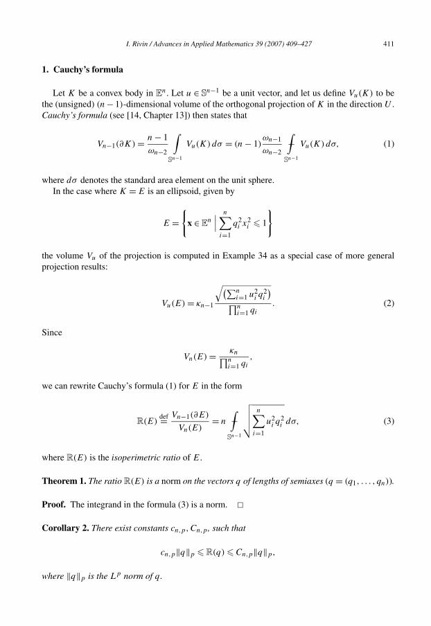
1. Cauchy’s formula
Let K be a convex body in En. Let u ∈ S
n−1 be a unit vector, and let us define Vu(K) to bethe (unsigned) (n− 1)-dimensional volume of the orthogonal projection of K in the direction U .Cauchy’s formula (see [14, Chapter 13]) then states that
Vn−1(∂K) = n − 1
ωn−2
∫Sn−1
Vu(K)dσ = (n − 1)ωn−1
ωn−2−∫
Sn−1
Vu(K)dσ, (1)
where dσ denotes the standard area element on the unit sphere.In the case where K = E is an ellipsoid, given by
E ={
x ∈ En
∣∣∣ n∑i=1
q2i x2
i � 1
}
the volume Vu of the projection is computed in Example 34 as a special case of more generalprojection results:
Vu(E) = κn−1
√(∑ni=1 u2
i q2i
)∏n
i=1 qi
. (2)
Since
Vn(E) = κn∏ni=1 qi
,
we can rewrite Cauchy’s formula (1) for E in the form
R(E)def= Vn−1(∂E)
Vn(E)= n −
∫Sn−1
√√√√ n∑i=1
u2i q
2i dσ, (3)
where R(E) is the isoperimetric ratio of E.
Theorem 1. The ratio R(E) is a norm on the vectors q of lengths of semiaxes (q = (q1, . . . , qn)).
Proof. The integrand in the formula (3) is a norm. �Corollary 2. There exist constants cn,p,Cn,p , such that
cn,p‖q‖p � R(q) � Cn,p‖q‖p,
where ‖q‖p is the Lp norm of q .

412 I. Rivin / Advances in Applied Mathematics 39 (2007) 409–427
Proof. Immediate (since all norms on a finite-dimensional Banach space are equivalent). �In the sequel we will find sharp bounds on the constants cn,p and Cn,p , but for the moment
observe that if ai = 1/qi , i = 1, . . . , n, then
‖q‖p =n∏
i=1
qiσ1/p
n−1
(a
p
1 , . . . , apn
), (4)
where σn−1 is the (n − 1)st elementary symmetric function. In particular, for p = 1, Corollary 2together with Eq. (4) gives the estimate of [12] (only for the 0th mean curvature integral andwith (for now) ineffective constants—the latter part will be remedied directly). To exploit theformula (3) fully, we will need a digression on computing spherical integrals.
2. Spherical integrals
In this section we will prove the following simple but very useful theorem.
Theorem 3. Let f (x1, . . . , xn) be a homogeneous function on En of degree d (in other words,
f (λx1, . . . , λxn) = λdf (x1, . . . , xn)). Then
�
(n + d
2
)−∫
Sn−1
f dσ = �
(n
2
)E
(f (X1, . . . ,Xn)
),
where X1, . . . ,Xn are independent random variables with probability density e−x2.
Proof. Let
E(f ) = −∫
Sn−1
f (x)dσ.
Let N(f ) be defined as E(f (X1, . . . ,X�)), where Xi is a Gaussian random variable withmean 0 and variance 1/2. (The probability density of Xi is given by n(x) = e−x2
.) The vari-ables X1, . . . ,Xn are independent. By definition,
N(f )(n) = cn
∫En
exp
(−
n∑i=1
x2i
)f (x1, . . . , xn) dx1 . . . dxn, (5)
where cn is such that
cn
∫n
exp
(−
n∑i=1
x2i
)dx1 . . . dxn = 1. (6)
E
I. Rivin / Advances in Applied Mathematics 39 (2007) 409–427 413
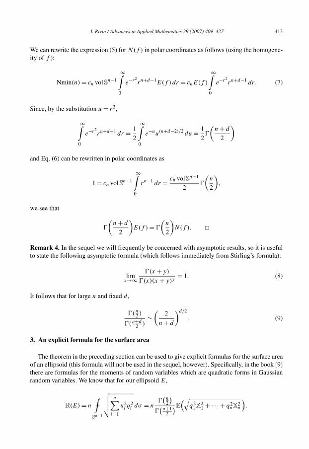
We can rewrite the expression (5) for N(f ) in polar coordinates as follows (using the homogene-ity of f ):
Nmin(n) = cn vol Sn−1
∞∫0
e−r2rn+d−1E(f )dr = cnE(f )
∞∫0
e−r2rn+d−1 dr. (7)
Since, by the substitution u = r2,
∞∫0
e−r2rn+d−1 dr = 1
2
∞∫0
e−uu(n+d−2)/2 du = 1
2�
(n + d
2
)
and Eq. (6) can be rewritten in polar coordinates as
1 = cn vol Sn−1
∞∫0
rn−1 dr = cn vol Sn−1
2�
(n
2
),
we see that
�
(n + d
2
)E(f ) = �
(n
2
)N(f ). �
Remark 4. In the sequel we will frequently be concerned with asymptotic results, so it is usefulto state the following asymptotic formula (which follows immediately from Stirling’s formula):
limx→∞
�(x + y)
�(x)(x + y)y= 1. (8)
It follows that for large n and fixed d ,
�(n2 )
�(n+d2 )
∼(
2
n + d
)d/2
. (9)
3. An explicit formula for the surface area
The theorem in the preceding section can be used to give explicit formulas for the surface areaof an ellipsoid (this formula will not be used in the sequel, however). Specifically, in the book [9]there are formulas for the moments of random variables which are quadratic forms in Gaussianrandom variables. We know that for our ellipsoid E,
R(E) = n −∫n−1
√√√√ n∑i=1
u2i q
2i dσ = n
�(
n2
)�
(n+1
2
)E
(√q2
1X21 + · · · + q2
nX2n
),
S

414 I. Rivin / Advances in Applied Mathematics 39 (2007) 409–427
where Xi is a Gaussian with variance 1/2. The expectation in the last expression is the 1/2thmoment of the quadratic form in Gaussian random variables, and so the results of [9, p. 62]apply verbatim, so that we obtain:
R(E) = n�
(n2
)�
(n+1
2
)�
( 12
)√α
∞∫0
1√z
n∑j=1
q2j
2(1 + αzq2j )
(n∏
j=1
(1 − q2
j z))−1/2
dz; (10)
note that α in the above formula can be any positive number (as long as |1 − αq2j | < 1, for all j .
This can also be expressed in terms of special functions. First, we need a definition.
Definition 5. Let a, b1, . . . , bn, c, x1, . . . , xn be complex numbers, with |xi | < 1, i = 1, . . . , n,�a > 0, �(c − a) > 0. We then define the Lauricella hypergeometric function FD(a;b1, . . . , bn;c;x1, . . . , xn) as follows:
FD(a;b1, . . . , bn; c;x1, . . . , xn)
= �(c)
�(a)�(c − a)
1∫0
ua−1(1 − u)c−a−1n∏
i=1
(1 − uxi)−bi du. (11)
We also have the series expansion
FD(a;b1, . . . , bn; c;x1, . . . , xn)
=∞∑
m1=0
. . .
∞∑mn=0
(a)m1+···+mn
∏ni=1(bi)mi
(c)m1+···+mn
n∏i=1
xmi
i
mi ! , (12)
valid whenever |xi | < 1, ∀i.
Now, we can write
R(E) = n�2
(n2
)�2
(n+1
2
)√α
×n∑
j=1
q2j
2FD
(1/2;η1j , . . . , ηnj ; n + 1
2;1 − αq2
1 , . . . ,1 − αq2n
), (13)
where ηij = 1/2 + δij , and α is a positive parameter satisfying |1 − αq2j | < 1.
4. Laws of large numbers
Many of the results in this section will require the following basic lemmas.
Lemma 6. Let F1, . . . ,Fn, . . . be a sequence of probability distributions whose first momentsconverge to μ and whose second moments converge to 0. Then the Fi converge to the Dirac deltafunction distribution centered on μ.
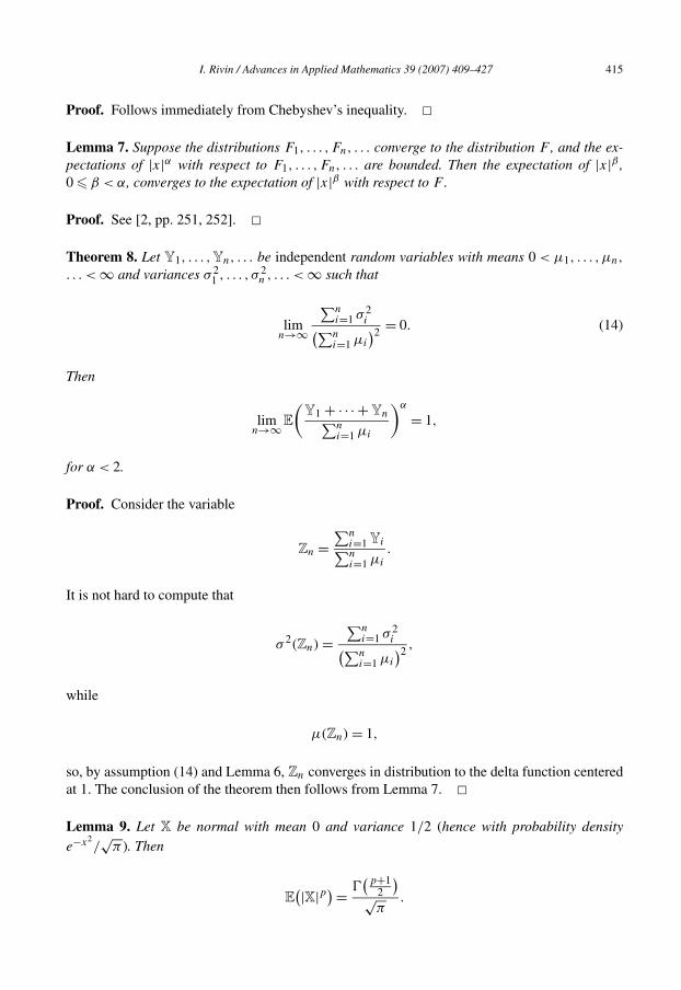
I. Rivin / Advances in Applied Mathematics 39 (2007) 409–427 415
Proof. Follows immediately from Chebyshev’s inequality. �Lemma 7. Suppose the distributions F1, . . . ,Fn, . . . converge to the distribution F , and the ex-pectations of |x|α with respect to F1, . . . ,Fn, . . . are bounded. Then the expectation of |x|β ,0 � β < α, converges to the expectation of |x|β with respect to F .
Proof. See [2, pp. 251, 252]. �Theorem 8. Let Y1, . . . ,Yn, . . . be independent random variables with means 0 < μ1, . . . ,μn,
. . . < ∞ and variances σ 21 , . . . , σ 2
n , . . . < ∞ such that
limn→∞
∑ni=1 σ 2
i(∑ni=1 μi
)2= 0. (14)
Then
limn→∞ E
(Y1 + · · · + Yn∑n
i=1 μi
)α
= 1,
for α < 2.
Proof. Consider the variable
Zn =∑n
i=1 Yi∑ni=1 μi
.
It is not hard to compute that
σ 2(Zn) =∑n
i=1 σ 2i(∑n
i=1 μi
)2,
while
μ(Zn) = 1,
so, by assumption (14) and Lemma 6, Zn converges in distribution to the delta function centeredat 1. The conclusion of the theorem then follows from Lemma 7. �Lemma 9. Let X be normal with mean 0 and variance 1/2 (hence with probability densitye−x2
/√
π ). Then
E(|X|p) = �
(p+12
)√
π.

416 I. Rivin / Advances in Applied Mathematics 39 (2007) 409–427
Proof.
E(|X|p) = 2√
π
∞∫0
xpe−x2dx = 1√
π
∞∫0
u(p−1)/2e−u = �(p+1
2
)√
π. �
Theorem 10.
−∫
Sn−1
‖u‖p dσ ∼ �(
n2
)�
(n+1
2
)(n�
(p+12
)√
π
) 1p
.
Proof. This follows immediately from the 1-homogeneity of the Lp norm, the results of Sec-tion 2, Theorem 8, and Lemma 9. �4.1. Asymptotics of R(E)
Theorem 11. Let q1, . . . , qn, . . . be a sequence of positive numbers such that
limn→∞
∑ni=1 q4
i(∑ni=1 q2
i
)2= 0.
Let En be the ellipsoid in En with semi-axes a1 = 1/q1, . . . , an = 1/qn. Then
limn→∞
�(
n+12
)�
(n2
) R(En)
n
√12
∑ni=1 q2
i
= 1.
Proof. The theorem follows immediately from Theorem 8 and the results of Section 2. �Corollary 12. Let a1, . . . , an, . . . be such that 0 < c1 � ai/aj � c2 < ∞, for any i, j . Let En bethe ellipsoid with semi-axes a1, . . . , an. Then
limn→∞
�(
n+12
)�
(n2
) R(En)
n
√12
∑ni=1
1a2i
= 1.
Proof. The quantities q1 = 1/a1, . . . , qn = 1/an, . . . clearly satisfy the hypotheses of Theo-rem 11. �5. General bounds on RRR(E)
We know that R(E) is a norm on the vector q = (q1, . . . , qn). Let us agree to write
‖q‖R
def= R(E)
n= −
∫n−1
√√√√ n∑i=1
q2i x2
i dσ,
S

I. Rivin / Advances in Applied Mathematics 39 (2007) 409–427 417
where q is the vector of inverses of the major semi-axes of E. We know that
cn‖q‖ � ‖q‖R � Cn‖q‖,
for some dimensional constants cn,Cn. In this section we will give sharp estimates on the cn
and Cn. These estimates will depend on the following observation.
Lemma 13. Let α1, . . . , αn be non-negative real numbers, and let
f (α1, . . . , αn) = −∫
Sn−1
√√√√ n∑i=1
αix2i dσ.
Then f (α) is a concave function of the vector α = (α1, . . . , αn).
Proof. The integrand is concave, since the square root is a concave function. The integral is thusalso concave, as a sum of concave functions. �Lemma 14. The ratio
‖q‖R
‖q‖is maximized when all of the qi are equal; it is minimized when q2 = · · · = qn = 0.
Proof. By homogeneity, we can assume that ‖q‖ = 1. Now, let αi = q2i . Letting
f (α) = ‖q‖R,
we see that f is a symmetric function, while Lemma 13 tells us that f (α) is a concave function.Since the set
S:n∑
i=1
αi = 1
is convex, we know that the maximum of f is attained at the point of maximum symmetry2
(αi = 1/n, for all i), and the minimum at an extreme point of S. By symmetry, any extreme pointwill do, for example (1,0, . . . ,0). �Corollary 15. The minimal value ( previously denoted by cn) of ‖q‖R/‖q‖ equals
−∫Sn
|x1|dσ = �(
n2
)√
π�(
n+12
) ,
2 Since the maximum of f is unique in a convex domain.
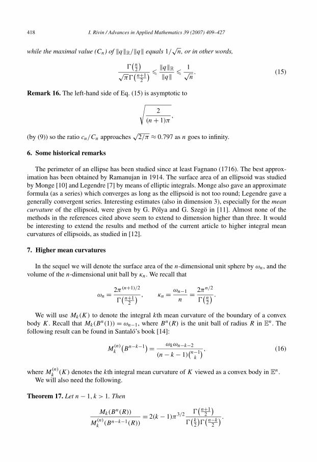
418 I. Rivin / Advances in Applied Mathematics 39 (2007) 409–427
while the maximal value (Cn) of ‖q‖R/‖q‖ equals 1/√
n, or in other words,
�(
n2
)√
π�(
n+12
) � ‖q‖R
‖q‖ � 1√n. (15)
Remark 16. The left-hand side of Eq. (15) is asymptotic to√2
(n + 1)π,
(by (9)) so the ratio cn/Cn approaches√
2/π ≈ 0.797 as n goes to infinity.
6. Some historical remarks
The perimeter of an ellipse has been studied since at least Fagnano (1716). The best approx-imation has been obtained by Ramanujan in 1914. The surface area of an ellipsoid was studiedby Monge [10] and Legendre [7] by means of elliptic integrals. Monge also gave an approximateformula (as a series) which converges as long as the ellipsoid is not too round; Legendre gave agenerally convergent series. Interesting estimates (also in dimension 3), especially for the meancurvature of the ellipsoid, were given by G. Pólya and G. Szegö in [11]. Almost none of themethods in the references cited above seem to extend to dimension higher than three. It wouldbe interesting to extend the results and method of the current article to higher integral meancurvatures of ellipsoids, as studied in [12].
7. Higher mean curvatures
In the sequel we will denote the surface area of the n-dimensional unit sphere by ωn, and thevolume of the n-dimensional unit ball by κn. We recall that
ωn = 2π(n+1)/2
�(
n+12
) , κn = ωn−1
n= 2πn/2
�(
n2
) .
We will use Mk(K) to denote the integral kth mean curvature of the boundary of a convexbody K . Recall that Mk(B
n(1)) = ωn−1, where Bn(R) is the unit ball of radius R in En. The
following result can be found in Santaló’s book [14]:
M(n)k
(Bn−k−1) = ωkωn−k−2
(n − k − 1)(n−1k
) , (16)
where M(n)k (K) denotes the kth integral mean curvature of K viewed as a convex body in E
n.We will also need the following.
Theorem 17. Let n − 1, k > 1. Then
Mk(Bn(R))
M(n)k (Bn−k−1(R))
= 2(k − 1)π3/2 �(
n+12
)�
(k2
)�
(n−k
2
) .
I. Rivin / Advances in Applied Mathematics 39 (2007) 409–427 419
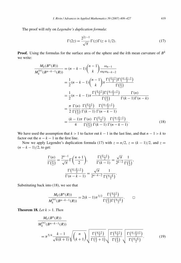
The proof will rely on Legendre’s duplication formula:
�(2z) = 22z−1
√π
�(z)�(z + 1/2). (17)
Proof. Using the formulas for the surface area of the sphere and the kth mean curvature of Bk
we write:
Mk(Bn(R))
M(n)k (Bn−k−1(R))
= (n − k − 1)
(n − 1
k
)ωn−1
ωkωn−k−2
= 1
2(n − k − 1)
(n − 1
k
)π
�(
k+12
)�
(n−k−1
2
)�
(n2
)= 1
2(n − k − 1)π
�(
k+12
)�
(n−k−1
2
)�
(n2
) �(n)
�(k − 1)�(n − k)
= π
2
�(n)
�(
n2
) �(
k+12
)�(k − 1)
�(
n−k−12
)�(n − k − 1)
= (k − 1)π
4
�(n)
�(
n2
) �(
k−12
)�(k − 1)
�(
n−k−12
)�(n − k − 1)
. (18)
We have used the assumption that k > 1 to factor out k − 1 in the last line, and that n − 1 > k tofactor out the n − k − 1 in the first line.
Now we apply Legendre’s duplication formula (17) with z = n/2, z = (k − 1)/2, and z =(n − k − 1)/2, to get:
�(n)
�(
n2
) = 2n−1
√π
�
(n + 1
2
),
�(
k−12
)�(k − 1)
=√
π
2k−2
1
�(
k2
) ,
�(
n−k−12
)�(n − k − 1)
=√
π
2n−k−2
1
�(
n−k2
) .
Substituting back into (18), we see that
Mk(Bn(R))
M(n)k (Bn−k−1(R))
= 2(k − 1)π3/2 �(
n+12
)�
(k2
)�
(n−k
2
) . �
Theorem 18. Let k > 1. Then
Mk(Bn(R))
M(n)k (Bn−k−1(R))
= π5/4 k − 1√k(k + 1)
√(n
k + 1
)√√√√ �(
n+12
)�
(n2 + 1
)√√√√�
(k+1
2
)�
(k2
)√√√√�
(n−k+1
2
)�
(n−k
2
) . (19)
420 I. Rivin / Advances in Applied Mathematics 39 (2007) 409–427
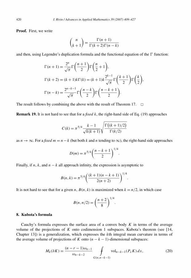
Proof. First, we write (n
k + 1
)= �(n + 1)
�(k + 2)�(n − k)
and then, using Legendre’s duplication formula and the functional equation of the � function:
�(n + 1) = 2n
√π
�
(n + 1
2
)�
(n
2+ 1
),
�(k + 2) = (k + 1)k�(k) = (k + 1)k2k−1
√π
�
(k + 1
2
)�
(k
2
),
�(n − k) = 2n−k−1
√π
�
(n − k
2
)�
(n − k + 1
2
).
The result follows by combining the above with the result of Theorem 17. �Remark 19. It is not hard to see that for a fixed k, the right-hand side of Eq. (19) approaches
C(k) = π5/4 k − 1√k(k + 1)
√�
((k + 1)/2
)�(k/2)
as n → ∞. For a fixed m = n−k (but both k and n tending to ∞), the right-hand side approaches
D(m) = π5/4(
n − k + 1
2
)1/4
.
Finally, if n, k, and n − k all approach infinity, the expression is asymptotic to
B(n, k) = π5/4(
(k + 1)(n − k + 1)
2(n + 2)
)1/4
.
It is not hard to see that for a given n, B(n, k) is maximized when k = n/2, in which case
B(n,n/2) =(
n + 2
8
)1/4
.
8. Kubota’s formula
Cauchy’s formula expresses the surface area of a convex body K in terms of the averagevolume of the projections of K onto codimension 1 subspaces. Kubota’s theorem (see [14,Chapter 13]) is a generalization, which expresses the kth integral mean curvature in terms ofthe average volume of projections of K onto (n − k − 1)-dimensional subspaces:
Mk(∂K) = (n − r − 1)ωn−1
ωn−k−2−∫
voln−k−1(PxK)dx, (20)
G(n,n−k−1)

I. Rivin / Advances in Applied Mathematics 39 (2007) 409–427 421
where G(n,n − k − 1) is the Grassmannian of (n − k − 1)-dimensional linear subspaces of En,
and Px is the projection onto the subspace x. In the special case where K is an ellipsoid E withaxes a1, . . . , an, Theorem 31 gives us several explicit expressions for the integrand in Kubota’sformula. For the purposes of the next theorem, Eq. (28b) will be the most useful.
Theorem 20. Let E be an ellipsoid with axes a1, . . . , an. Let ai, for a multi-index i =(i1, . . . , in−k−1) be defined as
ai =n−k−1∏
l=1
ail ,
and let
A =√∑
i
a2i ,
where the sum us taken over increasing multi-indices. Then
M(n)k
(Bk(1)
)A � Mk(E) �
Mk
(Bn(1)
)√(
nk+1
) A. (21)
Proof. The proof is identical to the proof of Lemma 14, except we use ai as variables. With thenormalization A = 1 (allowed by homogeneity) we see that the maximal case corresponds to theball of such a radius that ai = (
nn−k−1
)−1/2, for any multi-index i, and the minimum correspondsto a1 = · · · = an−k−1 = 1, while an−k = · · · = an = 0. �
The ratio of the right-hand side of the inequality (21) to the left-hand side is the subject ofTheorem 18 and Remark 19. As commented in the Remark, the ratio is bounded for any fixed k,and in the worst case (for k = n/2), the ratio grows like n1/4.
9. Some exterior algebra
Let V be a vector space, and let A be a linear transformation:
A ∈ Hom(V ,V ).
The exterior power∧k
V is the vector space spanned by multivectors of the form v1 ∧ . . . ∧ vk ,and so we define
k∧A ∈ Hom
( k∧V,
k∧V
)
by
k∧A(v1 ∧ . . . ∧ vk) = Av1 ∧ . . . ∧ Avk.
422 I. Rivin / Advances in Applied Mathematics 39 (2007) 409–427
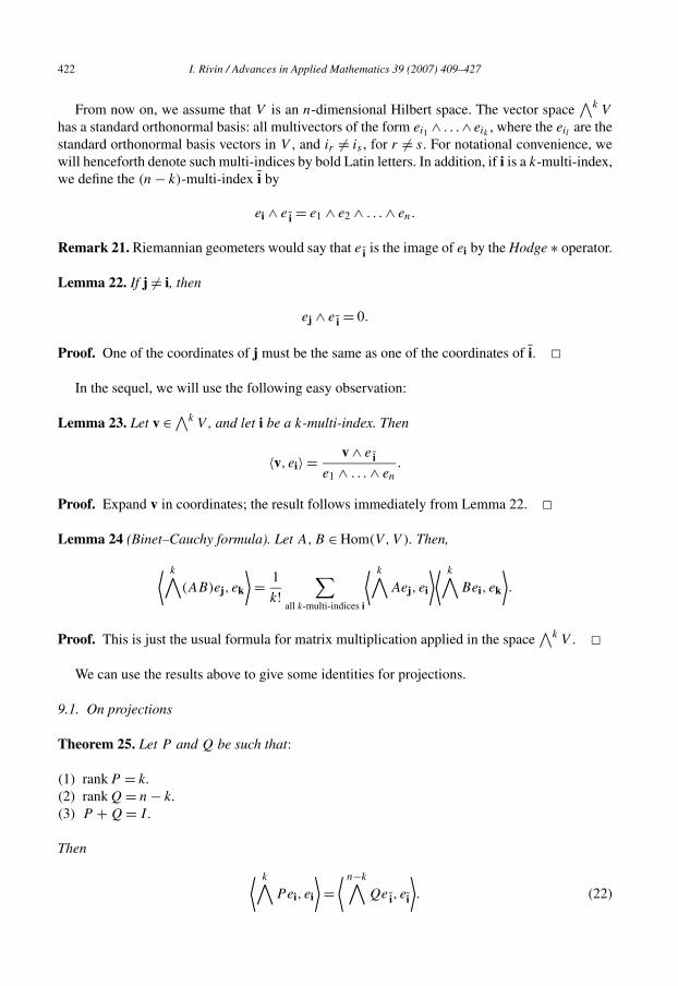
From now on, we assume that V is an n-dimensional Hilbert space. The vector space∧k
V
has a standard orthonormal basis: all multivectors of the form ei1 ∧ . . .∧ eik , where the eil are thestandard orthonormal basis vectors in V , and ir �= is , for r �= s. For notational convenience, wewill henceforth denote such multi-indices by bold Latin letters. In addition, if i is a k-multi-index,we define the (n − k)-multi-index i by
ei ∧ e i = e1 ∧ e2 ∧ . . . ∧ en.
Remark 21. Riemannian geometers would say that e i is the image of ei by the Hodge ∗ operator.
Lemma 22. If j �= i, then
ej ∧ e i = 0.
Proof. One of the coordinates of j must be the same as one of the coordinates of i. �In the sequel, we will use the following easy observation:
Lemma 23. Let v ∈ ∧kV , and let i be a k-multi-index. Then
〈v, ei〉 = v ∧ e i
e1 ∧ . . . ∧ en
.
Proof. Expand v in coordinates; the result follows immediately from Lemma 22. �Lemma 24 (Binet–Cauchy formula). Let A,B ∈ Hom(V ,V ). Then,
⟨ k∧(AB)ej, ek
⟩= 1
k!∑
all k-multi-indices i
⟨ k∧Aej, ei
⟩⟨ k∧Bei, ek
⟩.
Proof. This is just the usual formula for matrix multiplication applied in the space∧k
V . �We can use the results above to give some identities for projections.
9.1. On projections
Theorem 25. Let P and Q be such that:
(1) rankP = k.(2) rankQ = n − k.(3) P + Q = I .
Then
⟨ k∧Pei, ei
⟩=
⟨ n−k∧Qe i, ei
⟩. (22)

I. Rivin / Advances in Applied Mathematics 39 (2007) 409–427 423
Proof.
⟨ k∧Pei, ei
⟩=
∧kP ei ∧ ei
e1 ∧ en
=∧k
P ei ∧ ∧n−k(P + Q)ei
e1 ∧ en
=∧k
P ei ∧ ∧n−k(Q)e i
e1 ∧ en
=∧k
(P + Q)ei ∧ ∧n−k(Q)e i
e1 ∧ en
=∧k
ei ∧ ∧n−k(Q)e i
e1 ∧ en
=⟨ n−k∧
Qe i, e i
⟩,
where we have used the observation that∧l
P = 0, whenever l > rankP . �Suppose W is a subspace of V , and let w1, . . . ,wk be an orthonormal basis of W . Let Ω be the
matrix whose columns are the vectors (w1, . . . ,wk,0, . . . ,0) (padding Ω by zeros is not reallynecessary, but it will make the sequel slightly simpler notationally). We then have the following.
Lemma 26. Let P be the orthogonal projection onto W . Then
P = ΩΩt .
Proof. The proof is by direct computation: we will show that Q = ΩΩt is the sought-after pro-jector. First, let v be orthogonal to all of W . Then, it is clear that Ωtv = 0, and so Qv = 0. Now,consider Qwi . First, Ωtwi = ei . Now, for any matrix A, Aei is the ith column of A. In particular,Ωei = wi , and so Qwi = wi , for all i. It follows that Q is the sought-after projector. �Corollary 27. Let P and Ω be as above. Then
⟨ k∧Pei, ei
⟩=
⟨ k∧Ωei, ei
⟩2
.
Proof. This is an immediate consequence of Lemma 26 above and Lemma 24. �The following can be viewed as a generalization of the Pythagorean theorem.
Theorem 28 (Generalized Pythagorean theorem). Let Ω be as above. Then the sum of squaresof k × k minors of Ω equals 1.
Proof. By examination of the characteristic polynomial of P , the product of the non-zero eigen-values of P equals the sum of the principal k × k minors, which, by Corollary 27 equals the sumof squares of the k × k minors of Ω . However, since P is a projection, its non-zero eigenvaluesare all equal to 1. �Remark 29. A different approach to Theorem 28 can be found in E.L. Grinberg’s paper [4].

424 I. Rivin / Advances in Applied Mathematics 39 (2007) 409–427
10. How to compute the volume of a projected ellipsoid
First, consider a generalized ellipsoid E(A)—the image of the unit ball in Rn under a linear
transformation A of rank k. We would like to know the k-dimensional volume of E(A). Thesimplest situation is when
Aij ={
λi, i = j, i � k,
0, otherwise.(23)
In this case,
volk(E(A)
) = κk
k∏i=1
λi. (24)
The general case is not much different: any matrix A of rank k can be written as UΣV , whereV ∈ O(n), and U is in O(k) ⊂ O(n), while Σ is the diagonal matrix of type described inEq. (23); the diagonal entries of Σ are the singular values of A, which can be alternately de-scribed as the positive square roots of the (non-zero) eigenvalues of either AtA or AAt . Let usstate this as a theorem.
Theorem 30. Let E(A) be the image of the unit ball in Rn under a transformation A of rank k.
Then
volk(E(A)
) = κk
k∏i=1
σi, (25)
where σ1, . . . , σk are the singular values of A.
Now, we note that for a matrix M of rank k, the product of the non-zero eigenvalues of M
equals the sum of k × k principal minors of M (this is immediate by examining the characteristicpolynomial of M). Thus Eq. (25) can be rewritten as
vol2k(E(A)
) = κk
∑principal submatrices M of AtA
detM. (26)
This last form is superior to Eq. (25), since it expresses the square of the volume as a polynomialin the entries of A. We also note that the k × k principal minor Mi of a matrix M is somethingwe have already seen:
Mi =⟨ k∧
Mei, ei
⟩.
I. Rivin / Advances in Applied Mathematics 39 (2007) 409–427 425
10.1. How do we compute the volume of a projection of an ellipsoid?
Here we consider a special case: we take a non-degenerate ellipsoid E(A), where, for sim-plicity, A = diaga1, . . . , an, and we would like to compute the volume of the projection of E(A)
onto a k-dimensional subspace W with the associated projector P . In other words, we want tocompute the volume of E(PA). With the notation A = PA we note that AtA = APA. To usethe formula (26) we first note that if i is a multi-index, then we have the following expression forthe minors of AtA:
(APA)i = a2i Pi, (27)
where, if i = (i1, . . . , ik), then
ai =k∏
l=1
ail .
We then have the following.
Theorem 31 (Measure of ellipsoid projections). Let E be the ellipsoid
E ={
x ∈ Rn
∣∣∣ n∑i=1
x2i
a2i
� 1
}.
Let W be a subspace of Rn, with an orthonormal basis w1, . . . ,wk , and let the orthogonal
subspace W⊥ have the orthonormal basis wk+1, . . . ,wn. Let Ω be the n × k matrix whose rowsare the vectors w1, . . . ,wk . Let Ω⊥ be the n× (n− k) matrix whose rows are wk+1, . . . ,wn. Letthe projection onto W be denoted by P . Let the projection onto W⊥ be denoted by P ⊥. Then,the k-dimensional volume volk P (E) of the projection of E onto W can be expressed in anyone of the following ways (the sums in Eqs. (28a), (28b) are taken over nondecreasing k multi-indices i = (i1, . . . , ik), i1 � i2 � · · · � ik ; the sums in Eqs. (28c), (28d) over nondecreasing n−k
multi-indices i):
volk P (E) = κk
√∑Pia
2i , (28a)
volk P (E) = κk
√∑Ω2
i a2i , (28b)
volk P (E) = κk
n∏i=1
ai
√∑ P ⊥i
a2i
, (28c)
volk P (E) = ωk
n∏i=1
ai
√√√√∑ (Ω⊥
i
)2
a2i
. (28d)

426 I. Rivin / Advances in Applied Mathematics 39 (2007) 409–427
Proof. The expression (28a) follows immediately from Eq. (26). The expression (28b) followsfor Eq. (28a) and Corollary 27. The expression (28c) follows from Eq. (28a) and Theorem 22.The expression (28d) follows from Eq. (28c) and Corollary 27. �Remark 32. The last two expressions (28c) and (28d) in the above theorem are more useful whenk > n/2; the forms (28b) and (28d) are useful when the subspaces are given by their generatingvectors, while (28a) and (28c) are more useful when the subspaces are given by their projectors.
Example 33. Suppose k = 1, so we are projecting on a subspace spanned by a (unit) vectorv = (v1, . . . , vn). Then, the length of the projection of our ellipsoid is (according to Eq. (28b)
n∑i=1
v2i a
2i .
Example 34. Suppose k = n − 1, so we are projecting onto the orthogonal complement of thesubspace spanned by v of the previous example. Then, the (n − 1)-dimensional volume of theprojection of our ellipsoid is (according to Eq. (28d)):
κn−1
n∏i=1
ai
n∑j=1
v2j
a2i
.
This formula was previously obtained (by completely different methods) by Connelly and Ostroin [1].
11. Isoperimetric questions
Theorem 20 can be expressed as follows.
Let E be the set of ellipsoids such that the squares of the (n − k − 1)-dimensional vol-umes of the projections onto coordinate (n − k − 1)-dimensional subspaces equals 1. Thenthe largest value of Mk(E) for E ∈ E(A) is achieved by the n-dimensional ball (of radius(
nn−k−1
)−1/(n−k−1)), while the minimal value of Mk(E) is achieved by any (n − k − 1)-dimensional ellipsoid parallel to one of the coordinate subspaces.
It is natural to ask whether the above statement holds with the word “ellipsoid” replaced bythe word “convex body” throughout. I believe that the answer is in the affirmative, but it is clearthat the methods of this paper do not apply to this question in this generality.
Acknowledgments
The author would like to thank NSF DMS for partial support. He would also like to thank theHebrew University of Jerusalem for its hospitality and the Lady Davis Fellowship Trust for itssupport during the final revision of this paper. Parts of this paper appeared as the preprint [13];the author would like to thank Warren D. Smith on comments on a previous version of this pa-per.The author would also like to thank Princeton University, New York University, and Unversité

I. Rivin / Advances in Applied Mathematics 39 (2007) 409–427 427
Paul Sabatier for their hospitality.The author would also like to thank Franck Barthe for simpli-fying the arguments in Section 5, and thus obtaining the sharp bounds presented in that section,and also in Theorem 20 (which uses the same argument). Barthe also found an integral-geometricproof of much of Theorem 31. Last, but not least, the author would like to thank the referee forhis (or her) thorough reading of a previous version of the manuscript.
References
[1] R. Connelly, S.J. Ostro, Ellipsoids and lightcurves, Geom. Dedicata 17 (1) (1984) 87–98.[2] W. Feller, An Introduction to Probability Theory and Its Applications. vol. II, second ed., Wiley, New York, 1971.[3] H. Furstenberg, I. Tzkoni, Spherical functions and integral geometry, Israel J. Math. 10 (1971) 327–338.[4] E.L. Grinberg, On images of Radon transforms, Duke Math. J. 52 (4) (1985) 939–972.[5] H. Guggenheimer, A formula of Furstenberg–Tzkoni type, Israel J. Math. 14 (1973) 281–282.[6] R. Howard, The kinematic formula in Riemannian homogeneous spaces, Mem. Amer. Math. Soc. 106 (509) (1993),
vi+69.[7] A.M. Legendre, Traité des Fonctions Elliptiques et Intégrales Eulériennes avec de tables pour en faciliter le calcul
numérique, vol. 1, Huzard–Courcier, Paris, 1825.[8] E. Lutwak, On some ellipsoid formulas of Busemann, Furstenberg and Tzkoni, Guggenheimer, and Petty, J. Math.
Anal. Appl. 159 (1) (1991) 18–26.[9] A.M. Mathai, S.B. Provost, Quadratic Forms in Random Variables, Statist. Textbooks Monographs, vol. 126,
Dekker, New York, 1992. Theory and applications.[10] G. Monge, Feuilles d’analyse appliquée à la géometrie, vol. 19, Paris, an. 9.[11] G. Pólya, G. Szegö, Inequalities for the capacity of a condenser, Amer. J. Math. 67 (1945) 1–32.[12] I. Rivin, Simple estimates on ellipsoid measures, technical report, math.MG/0306085, 2003, arXiv.org.[13] I. Rivin, Spheres and minima, technical report, math.PR/0305252, 2003, arXiv.org.[14] L.A. Santaló, Integral Geometry and Geometric Probability, second ed., Cambridge Math. Lib., Cambridge Univ.
Press, Cambridge, 2004. With a foreword by Mark Kac.