Embed Size (px)
Citation preview
Algorithms for Ellipsoids
Stephen B. PopeSibley School of Mechanical & Aerospace Engineering
Cornell UniversityIthaca, New York 14853
Report: FDA-08-01February 2008
Abstract
We describe a number of algorithms to perform basic geometric operationson ellipsoids in n spatial dimensions, for n ≥ 1. These algorithms are im-plemented in ELL LIB, a library of Fortran subroutines. With E, E1 andE2 being given ellipsoids, and p a given point, the tasks considered include:determine the point in E which is closest to p or furthest from p; grow orshrink E so that its boundary intersects p; project E onto a given affinespace; determine a separating hyperplane between E1 and E2; determine anellipsoid (of small volume) which covers E1 and E2.
Contents
1 Introduction 3
2 Representation of ellipsoids 3
3 Summary of routines 5
4 Useful preliminary results 54.1 Linear transformation . . . . . . . . . . . . . . . . . . . . . . . 64.2 Quadratic minimization . . . . . . . . . . . . . . . . . . . . . 84.3 Householder matrix . . . . . . . . . . . . . . . . . . . . . . . . 84.4 Rank-one modification . . . . . . . . . . . . . . . . . . . . . . 9
5 Smallest and largest principal semi-axes of E 10
6 Is the point x covered by E? 12
7 Relative distance to the boundary of E 12
8 Nearest point in E to a given point 13
9 Furthest point in E to a given point 14
10 Minimum-volume ellipsoid covering E and p 1410.1 Householder matrix algorithm . . . . . . . . . . . . . . . . . . 1410.2 Rank-one modification algorithm . . . . . . . . . . . . . . . . 1710.3 Behavior . . . . . . . . . . . . . . . . . . . . . . . . . . . . . . 17
11 Shrink E based on a given point 1811.1 Maximum-volume algorithm . . . . . . . . . . . . . . . . . . . 19
11.1.1 Algorithm . . . . . . . . . . . . . . . . . . . . . . . . . 1911.1.2 Behavior . . . . . . . . . . . . . . . . . . . . . . . . . . 19
11.2 Near-content algorithm . . . . . . . . . . . . . . . . . . . . . . 2011.2.1 Algorithm . . . . . . . . . . . . . . . . . . . . . . . . . 2111.2.2 Behavior . . . . . . . . . . . . . . . . . . . . . . . . . . 22
11.3 Conservative algorithm . . . . . . . . . . . . . . . . . . . . . . 2211.3.1 Algorithm: reduction to 2D . . . . . . . . . . . . . . . 2411.3.2 Algorithm: solution in 2D . . . . . . . . . . . . . . . . 27
1
12 Orthogonal projection of E onto a given line 29
13 Orthogonal projection of E onto an affine space 30
14 Generate an ellipsoid which does not cover any specifiedpoints 32
15 Separating hyperplane of two ellipsoids 34
16 Pair covering query 36
17 Shrink ellipsoid so that it is covered by a concentric ellipsoid 36
18 Ellipsoid that covers two given ellipsoids 3818.1 Spheroid algorithm . . . . . . . . . . . . . . . . . . . . . . . . 3818.2 Covariance algorithm . . . . . . . . . . . . . . . . . . . . . . . 3918.3 Iterative algorithm . . . . . . . . . . . . . . . . . . . . . . . . 41
18.3.1 Stage 1 . . . . . . . . . . . . . . . . . . . . . . . . . . . 4118.3.2 Stage 2 . . . . . . . . . . . . . . . . . . . . . . . . . . . 4118.3.3 Stage 3 . . . . . . . . . . . . . . . . . . . . . . . . . . . 4118.3.4 Stage 4 . . . . . . . . . . . . . . . . . . . . . . . . . . . 4218.3.5 Stage 5 . . . . . . . . . . . . . . . . . . . . . . . . . . . 4418.3.6 Stage 6 . . . . . . . . . . . . . . . . . . . . . . . . . . . 4518.3.7 Mutual covering . . . . . . . . . . . . . . . . . . . . . . 4518.3.8 Discussion . . . . . . . . . . . . . . . . . . . . . . . . . 46
19 Conclusions 46
20 Acknowledgments 46
2
1 Introduction
In this paper we describe a number of algorithms to perform basic geometricoperations on ellipsoids. These algorithms have been implemented in Fortranroutines which are contained in the library ELL LIB, which is available athttp://eccentric.mae.cornell.edu/∼tcg/ELL LIB.
Ellipsoids arise in numerous computational problems. The algorithmsand routines described here have been developed specifically for use in thein situ adaptive tabulation (ISAT) algorithm (Pope 1997).
In Sec. 2 we consider different mathematical representations of an ellipsoidE in <n, for n ≥ 1. For n = 1, E is a line segment; for n = 2, E is an ellipse;for n = 3, E is an ellipsoid; and for n > 3, E is a hyper-ellipsoid. Forsimplicity we generally refer to E (for all n ≥ 1) as an ellipsoid.
A summary of the routines in ELL LIB is provided in Sec. 3. Follow-ing some preliminary results in Sec. 4, the algorithms used are described inSecs. 5–18.
2 Representation of ellipsoids
There are many ways to represent ellipsoids, with the different ways arisingnaturally in different circumstances. In this section we show the relationsbetween the different representations.
Let the ellipsoid E be centered at c; let the columns of the n×n orthogonalmatrix U be unit vectors in the directions of E’s principal axes; and let Σbe the diagonal matrix (with diagonal elements Σii = σi) such that 1/σi isthe length of the ith principal semi-axis. We assume that the principle axesare finite and strictly positive, i.e., 0 < σi < ∞. Then E is given by
E ≡ {x | (x− c)TUΣ2UT (x− c) ≤ 1}. (1)
This may alternatively be expressed as
E ≡ {x | ‖ΣUT (x− c)‖ ≤ 1}. (2)
or, from the definition w ≡ ΣUT (x− c),
E ≡ {x |x = c + UΣ−1w, ‖w‖ ≤ 1}. (3)
The above three definitions can be re-expressed in terms of different re-lated matrices. Let A be the matrix
3
A ≡ UΣ2UT , (4)
appearing in Eq.(1). Evidently A is symmetric positive definite; its eigen-vectors are the columns of U and its eigenvalues are λi = σ2
i . We denoteby Λ = Σ2 the diagonal matrix of eigenvalues. Thus Eqs. (1)–(3) can be
trivially re-written by substituting Λ12 for Σ; or less trivially in terms of A
asE ≡ {x | (x− c)TA(x− c) ≤ 1}, (5)
E ≡ {x | ‖A 12 (x− c)‖ ≤ 1}, (6)
E ≡ {x |x = c + A− 12w, ‖w‖ ≤ 1}. (7)
Let B be a non-singular square matrix, which we use to form A as
A = BBT , (8)
and let the SVD of B beB = UΣVT . (9)
Note that we have from Eq.(9),
A = BBT = UΣ2UT , (10)
consistent with Eq.(4), and showing that there is a family of matrices Byielding the same matrix A, namely B = UΣVT for given U and Σ butarbitrary orthogonal V. In terms of B, Eqs. (1)–(3) can be reexpressed as
E ≡ {x | (x− c)TBBT (x− c) ≤ 1}, (11)
E ≡ {x | ‖BT (x− c)‖ ≤ 1}, (12)
E ≡ {x |x = c + B−Tw, ‖w‖ ≤ 1}, (13)
with a different definition of w.The matrix B can also be factored as
B = LQ, (14)
4
where L is lower triangular with positive diagonal elements and Q is orthog-onal. Thus we obtain
A = BBT = LLT , (15)
showing that L is the Cholesky factorization of A. The definitions of E interms of B apply equally in terms of L, i.e.,
E ≡ {x | (x− c)TLLT (x− c) ≤ 1}, (16)
E ≡ {x | ‖LT (x− c)‖ ≤ 1}, (17)
E ≡ {x |x = c + L−Tw, ‖w‖ ≤ 1}. (18)
Computationally it is most efficient to use the Cholesky representationof the ellipsoid in terms of c and L, and to store L in packed format. InELL LIB, routines with names starting ell use this representation, while thosewith names starting ellu represent L in unpacked format.
In the algorithms described below, it often happens that an ellipsoid E1
given by c1 and L1 is modified to yield an ellipsoid E2 which is known interms of c2 and B2 (i.e., a full matrix). The representation in terms of L2
is efficiently and accurately computed by the LQ algorithm. It is stressedthat it is much more accurate to obtain L2 from the LQ algorithm than fromthe Cholesky decomposition of A = B2B
T2 . All of the algorithms described
below use the LQ algorithms and avoid forming A.The following table shows various routines in ELL LIB that can be used
to transform between one representation of an ellipsoid and another. In thistable, A denotes the lower triangle of the symmetric matrix A, while allother symbols have the meanings given above.
3 Summary of routines
Table 2 summarizes the tasks performed by the principal routines in ELL LIB.Here E, E1 and E2 denote given ellipsoids, and p denotes a given point.
4 Useful preliminary results
In this Section we give some general results that are used in the subsequentsections.
5
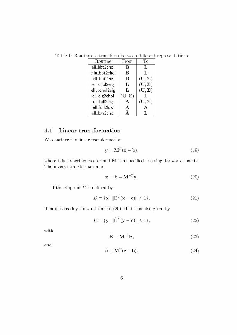
Table 1: Routines to transform between different representationsRoutine From To
ell bbt2chol B Lellu bbt2chol B Lell bbt2eig B (U,Σ)ell chol2eig L (U,Σ)ellu chol2eig L (U,Σ)ell eig2chol (U,Σ) Lell full2eig A (U,Σ)ell full2low A Aell low2chol A L
4.1 Linear transformation
We consider the linear transformation
y = MT (x− b), (19)
where b is a specified vector and M is a specified non-singular n×n matrix.The inverse transformation is
x = b + M−Ty. (20)
If the ellipsoid E is defined by
E ≡ {x | ‖BT (x− c)‖ ≤ 1}, (21)
then it is readily shown, from Eq.(20), that it is also given by
E = {y | ‖BT(y − c)‖ ≤ 1}, (22)
withB ≡ M−1B, (23)
andc ≡ MT (c− b). (24)
6
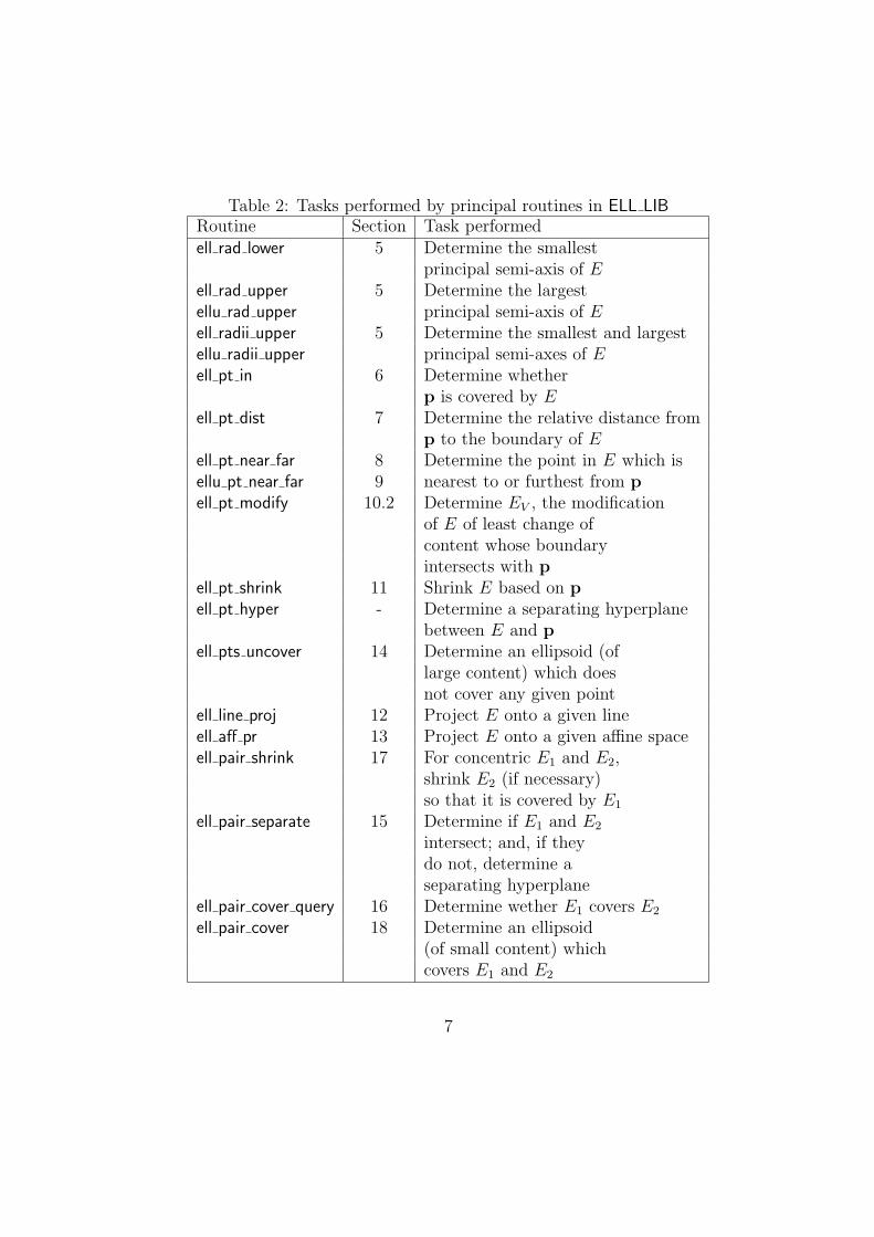
Table 2: Tasks performed by principal routines in ELL LIBRoutine Section Task performedell rad lower 5 Determine the smallest
principal semi-axis of Eell rad upper 5 Determine the largestellu rad upper principal semi-axis of Eell radii upper 5 Determine the smallest and largestellu radii upper principal semi-axes of Eell pt in 6 Determine whether
p is covered by Eell pt dist 7 Determine the relative distance from
p to the boundary of Eell pt near far 8 Determine the point in E which isellu pt near far 9 nearest to or furthest from pell pt modify 10.2 Determine EV , the modification
of E of least change ofcontent whose boundaryintersects with p
ell pt shrink 11 Shrink E based on pell pt hyper - Determine a separating hyperplane
between E and pell pts uncover 14 Determine an ellipsoid (of
large content) which doesnot cover any given point
ell line proj 12 Project E onto a given lineell aff pr 13 Project E onto a given affine spaceell pair shrink 17 For concentric E1 and E2,
shrink E2 (if necessary)so that it is covered by E1
ell pair separate 15 Determine if E1 and E2
intersect; and, if theydo not, determine aseparating hyperplane
ell pair cover query 16 Determine wether E1 covers E2
ell pair cover 18 Determine an ellipsoid(of small content) whichcovers E1 and E2
7
4.2 Quadratic minimization
Several of the algorithms described below depend on the solution to the fol-lowing problem: determine a vector x which minimizes the quadratic function
g(x) ≡ 12xTAx + bTx, (25)
subject toxTx ≤ δ2, (26)
where δ, b and A are a given scalar, vector, and symmetric matrix, re-spectively. Such problems are efficiently solved by the routine dgqt fromMINPACK-2 (see Averick et al. 1993).
4.3 Householder matrix
Given a vector p with p ≡ ‖p‖ > 0, the corresponding Householder matrixH(p) is defined by
H = I− 2vvT , (27)
where v is the unit vector
v1 = [(1 + |p1|)/(2p)]12 ,
vi =sign (p1)pi
2v1p, for i ≥ 2. (28)
It is readily shown that H has the following properties (not all independent):
1. H is symmetric: HT = H.
2. H is orthogonal: HTH = I.
3. The first column of H is parallel (or anti-parallel) to p.
4. All columns of H except the first are orthogonal to p.
5. H maps p to the first axis: Hp = pe1.
Given p, the routine ell house returns v.
8
4.4 Rank-one modification
Let E be an ellipsoid centered at the origin (i.e., c = 0), given in terms ofthe positive symmetric definite matrix A, which has SVD A = UΣ2UT , andCholesky decomposition A = LLT . For a given vector w and scalar ρ, let Fbe the rank-one modification of A:
F = A + ρwwT . (29)
We require F to be positive symmetric definite, which in turn requires ρto exceed a critical value ρ0 (ρ0 < 0) above which all eigenvalues of F arepositive (see item 7 below). Then, the modified ellipsoid E ′ is defined by
E ′ ≡ {x |xTFx ≤ 1}. (30)
The following results are readily obtained:
1. For ρ ≥ 0, xTFx is greater than or equal to xTAx, and hence E coversE ′.
2. For ρ ≤ 0, xTFx is less than or equal to xTAx, and hence E ′ coversE.
3. The eigenvalues of F are interlaced with those of A (see Golub andVan Loan 1996, Sec. 8.5.3). Hence the lengths of the principal axes ofE and E ′ are also interlaced.
4. With z ≡ ΣUTx, we have xTAx = zTz, so that E is the unit ball inz-space. Correspondingly, E ′ is given by
E ′ = {z | zT (I + ρwwT )z ≤ 1}. (31)
wherew = Σ−1UTw. (32)
Thus in z-space, one principal semi-axis of E ′ is (1 + ρ|w|2)− 12 w/|w|,
and the others are orthogonal unit vectors.
5. Similarly, with y ≡ LTx, we have xTAx = yTy, so that E is the unitball in y-space. Correspondingly, E ′ is given by
E ′ = {y |yT (I + ρwwT )y ≤ 1}. (33)
wherew = L−1w. (34)
9
6. The rank-one modifications to the identity appearing in Eq.(31) hasthe symmetric square root
I + ρwwT = G2 = (I + αwwT )(I + αwwT ) (35)
where α and ρ are related by
ρ = 2α + α2|w|2, (36)
α = (±{1 + ρ|w|2} 12 − 1)/|w|2. (37)
The matrix in Eq.(33) has a similar square root, with the same valueof α, since |w| = |w|.
7. The critical value of ρ is
ρ0 = −1/|w|2, (38)
corresponding to the smallest value of ρ for which α is real.
5 Smallest and largest principal semi-axes of
E
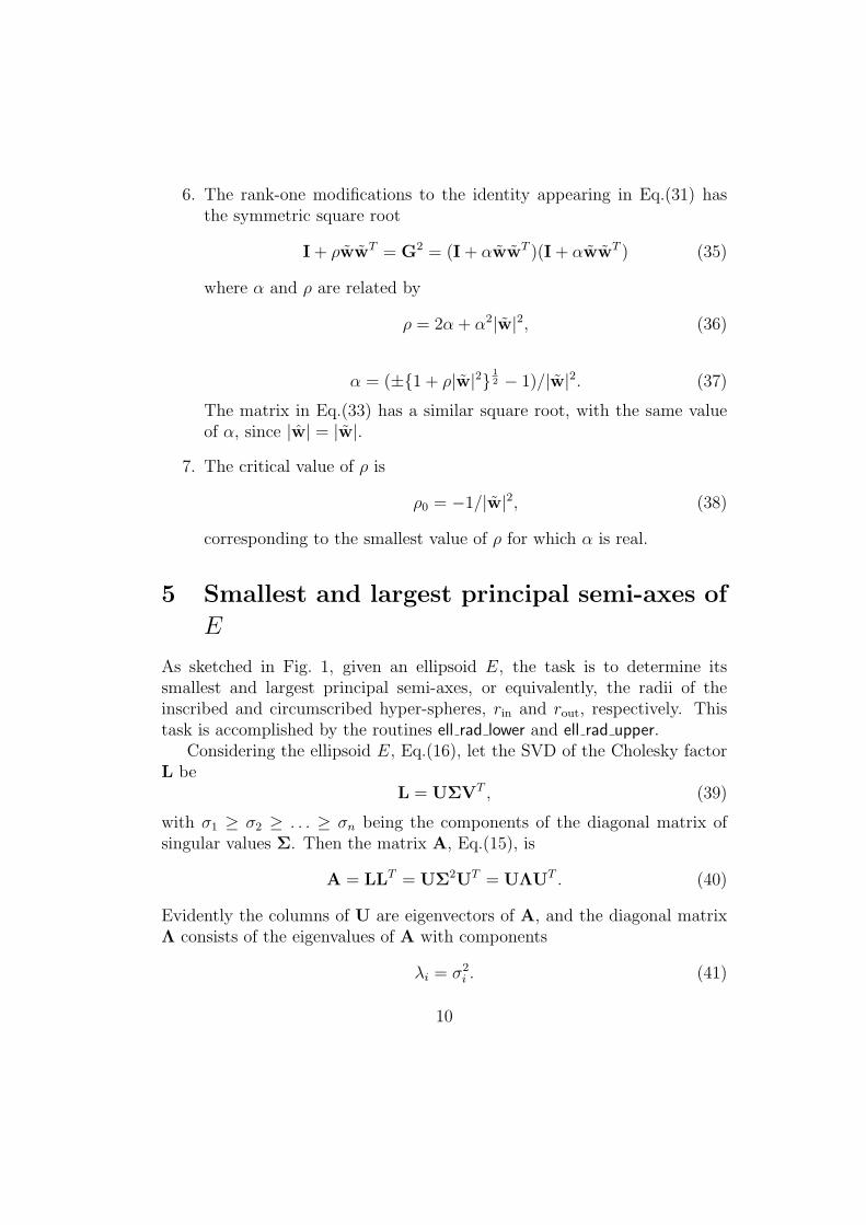
As sketched in Fig. 1, given an ellipsoid E, the task is to determine itssmallest and largest principal semi-axes, or equivalently, the radii of theinscribed and circumscribed hyper-spheres, rin and rout, respectively. Thistask is accomplished by the routines ell rad lower and ell rad upper.
Considering the ellipsoid E, Eq.(16), let the SVD of the Cholesky factorL be
L = UΣVT , (39)
with σ1 ≥ σ2 ≥ . . . ≥ σn being the components of the diagonal matrix ofsingular values Σ. Then the matrix A, Eq.(15), is
A = LLT = UΣ2UT = UΛUT . (40)
Evidently the columns of U are eigenvectors of A, and the diagonal matrixΛ consists of the eigenvalues of A with components
λi = σ2i . (41)
10
E
rin
rout
Figure 1: Sketch of an ellipsoid E showing the radii, rin and rout of the inscribedand circumscribed hyper-spheres.
The principal semi-axes are given by ri = λ− 1
2i = σ−1
i . Thus the smallestprinciple semi-axis is
rin = [max(λi)]− 1
2 , (42)
and the largest isrout = [min(λi)]
− 12 . (43)
The most stable way to compute rin is as rin = 1/σ1, where σ1 is obtainedfrom the SVD of L, and similarly for rout. The routine ell radii determinesboth rin and rout using the SVD.
The routines ell rad lower and ell rad upper determine rin and rout at sig-nificantly lower computational cost, but with less accuracy. Given L, theroutine ell rad lower determines rin via Eq.(42), using the LAPACK routinedsyevx to compute the largest eigenvalue of A.
The routine ell rad upper determines rout via quadratic minimization. Sincerout is the furthest distance from the center to any point on the ellipsoid wehave that r2
out is the maximum of rT r subject to
rTAr ≤ 1. (44)
By defining y = LT r, this can be put in the standard form of a quadraticminimization problem: −r2
out is the minimum of
−yTL−1L−Ty, (45)
11
subject toyTy ≤ 1. (46)
6 Is the point x covered by E?
Given a point x and an ellipsoid E (in terms of c and L), the task is todetermine whether E covers x. This is readily determined (by the routineell pt in) through the definition of E given by Eq.(17). That is, E covers xif the quantity
s ≡ ‖LT (x− c)‖, (47)
is less than or equal to unity.
7 Relative distance to the boundary of E
Given an ellipsoid E (in terms of c and L) and a point p (p 6= c), let b bethe intersection of the ray c-p with the boundary of E. The relative distances to the boundary is defined by:
s ≡ |b− c|/|p− c|. (48)
Now the boundary point satisfies
‖LT (b− c)‖ = 1, (49)
and we haveb− c = s (p− c). (50)
Hence, s is determined as
s = ‖LT (p− c)‖−1. (51)
The routine ell pt dist determines s.It may be noted that the three cases s < 1, s = 1 and s > 1 correspond,
respectively, to: p not being covered by E; p being on the boundary of E;and, p being covered by E.
12
E
p
n
f
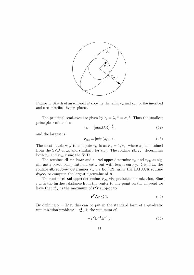
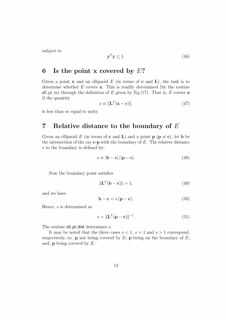
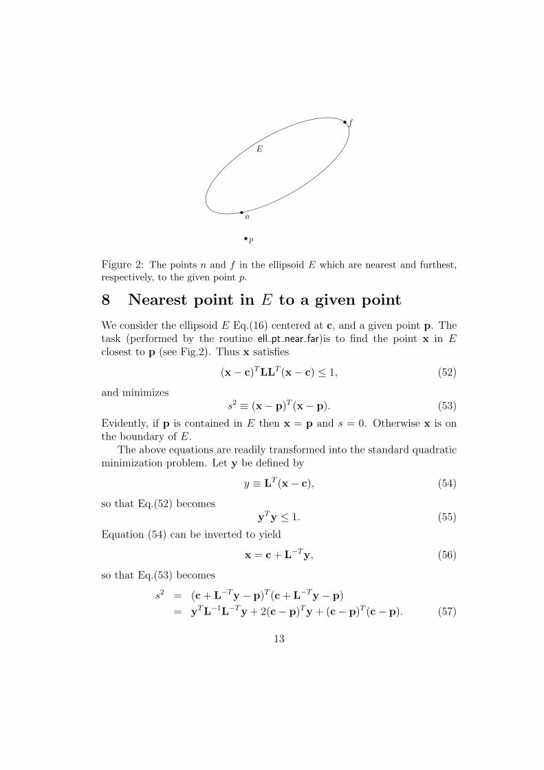
Figure 2: The points n and f in the ellipsoid E which are nearest and furthest,respectively, to the given point p.
8 Nearest point in E to a given point
We consider the ellipsoid E Eq.(16) centered at c, and a given point p. Thetask (performed by the routine ell pt near far)is to find the point x in Eclosest to p (see Fig.2). Thus x satisfies
(x− c)TLLT (x− c) ≤ 1, (52)
and minimizess2 ≡ (x− p)T (x− p). (53)
Evidently, if p is contained in E then x = p and s = 0. Otherwise x is onthe boundary of E.
The above equations are readily transformed into the standard quadraticminimization problem. Let y be defined by
y ≡ LT (x− c), (54)
so that Eq.(52) becomesyTy ≤ 1. (55)
Equation (54) can be inverted to yield
x = c + L−Ty, (56)
so that Eq.(53) becomes
s2 = (c + L−Ty − p)T (c + L−Ty − p)
= yTL−1L−Ty + 2(c− p)Ty + (c− p)T (c− p). (57)
13
Thus y is obtained via dgqt by minimizing
χ ≡ 12yTL−1L−Ty + (c− p)Ty, (58)
subject to ‖y‖ ≤ 1; and then x is obtained from Eq.(56).
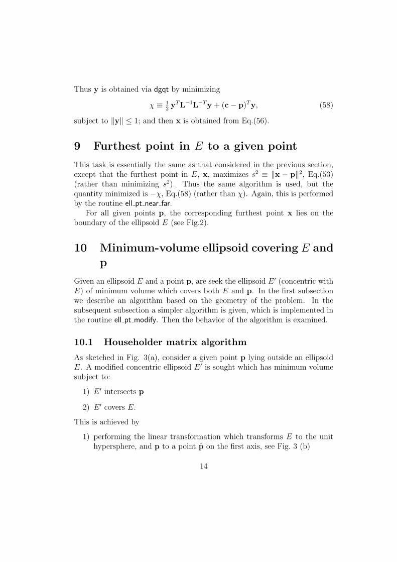
9 Furthest point in E to a given point
This task is essentially the same as that considered in the previous section,except that the furthest point in E, x, maximizes s2 ≡ ‖x − p‖2, Eq.(53)(rather than minimizing s2). Thus the same algorithm is used, but thequantity minimized is −χ, Eq.(58) (rather than χ). Again, this is performedby the routine ell pt near far.
For all given points p, the corresponding furthest point x lies on theboundary of the ellipsoid E (see Fig.2).
10 Minimum-volume ellipsoid covering E and
p
Given an ellipsoid E and a point p, are seek the ellipsoid E ′ (concentric withE) of minimum volume which covers both E and p. In the first subsectionwe describe an algorithm based on the geometry of the problem. In thesubsequent subsection a simpler algorithm is given, which is implemented inthe routine ell pt modify. Then the behavior of the algorithm is examined.
10.1 Householder matrix algorithm
As sketched in Fig. 3(a), consider a given point p lying outside an ellipsoidE. A modified concentric ellipsoid E ′ is sought which has minimum volumesubject to:
1) E ′ intersects p
2) E ′ covers E.
This is achieved by
1) performing the linear transformation which transforms E to the unithypersphere, and p to a point p on the first axis, see Fig. 3 (b)
14
� �� �
��� �� �
� �� �
�
� E ′
(a)
(c) (d)
(b)p
p
c
c
E p
p
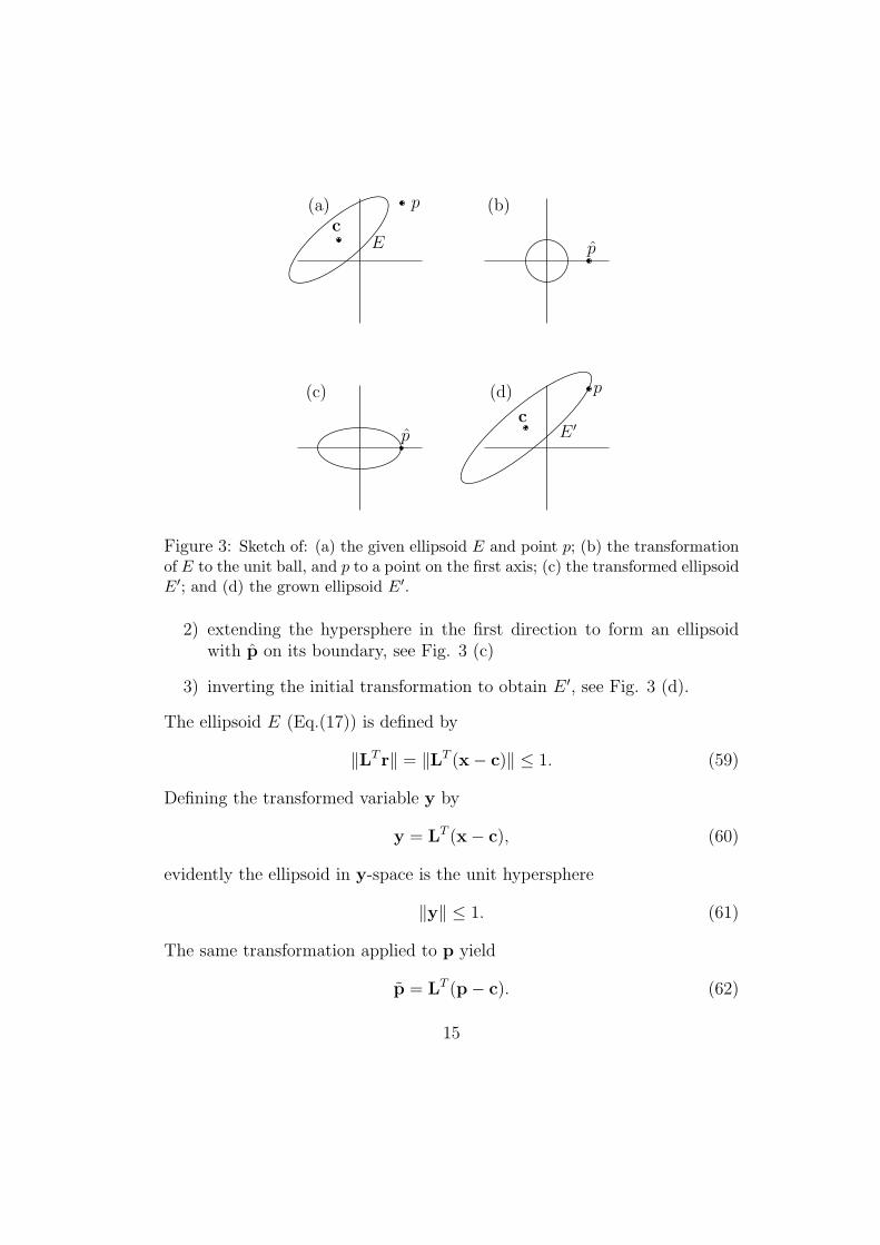
Figure 3: Sketch of: (a) the given ellipsoid E and point p; (b) the transformationof E to the unit ball, and p to a point on the first axis; (c) the transformed ellipsoidE′; and (d) the grown ellipsoid E′.
2) extending the hypersphere in the first direction to form an ellipsoidwith p on its boundary, see Fig. 3 (c)
3) inverting the initial transformation to obtain E ′, see Fig. 3 (d).
The ellipsoid E (Eq.(17)) is defined by
‖LT r‖ = ‖LT (x− c)‖ ≤ 1. (59)
Defining the transformed variable y by
y = LT (x− c), (60)
evidently the ellipsoid in y-space is the unit hypersphere
‖y‖ ≤ 1. (61)
The same transformation applied to p yield
p = LT (p− c). (62)
15
There is an orthogonal matrix Q which transforms p to a point on the1-axis; that is,
p = QT p = QTLT (p− c), (63)
wherepi = pδi1, (64)
and p = ‖p‖. It is readily shown that Q is simply the Householder matrixQ = H(p). The same transformation applied to E yields the unit ball
zTz ≤ 1, (65)
wherez = QTLT (x− c). (66)
This ball and the point p (pi ≡ pδi1) are shown in Fig. 3 (b). The next stepis to define the modified ellipse E ′ in z-space, as shown in Fig. 3 (c). Thisellipsoid is
zTΛ2z ≤ 1, (67)
whereΛ2
ij = δij + δi1δj1(p−2 − 1). (68)
Transforming back to the original space, we obtain the equation for E ′
(see Fig. 3 (d)):(x− c)TLQΛ2QTLT (x− c) ≤ 1, (69)
or(x− c)TL′L′T (x− c) ≤ 1. (70)
Thus the modified ellipsoid E ′ has center c and Cholesky matrix L′ given by
L′L′T = LQΛ2QTLT
= (LQΛ)(LQΛ)T . (71)
In summary, given the ellipsoid E (in terms of c and L) and the point p,then p is determined by Eq.(62), v by Eq.(28), Q by Eq.(27), Λ2 by Eq.(68),and finally the Cholesky matrix of the modified ellipsoid E ′ is determined byEq.(71).
16
10.2 Rank-one modification algorithm
Following from Eqs.(61) and (62), in y-space, the modified ellipsoid E ′ is theunit ball extended to intersect the point p. Thus, based on the results ofSec. 4.4, we have
E ′ = {y |yTG2y ≤ 1}, (72)
whereG = I + γppT , (73)
and γ (determined by the condition pTG2p = 1) is
γ =
(1
|p| − 1
)1
|p|2 . (74)
Thus, in place of Eq.(71), the Cholesky matrix L′ can be obtained as
L′L′T = (LG)(LG)T . (75)
This algorithm is implemented in the routine ell pt modify.
10.3 Behavior
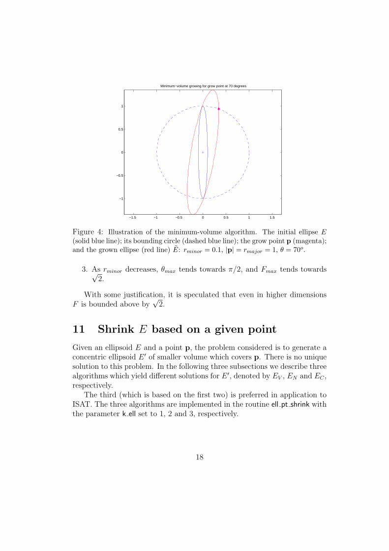
Test are reported for the minimum-volume growing algorithm. The tests arein two dimensions and are based on an initial ellipsoid E (centered at theorigin and aligned with the coordinate axes). The length of the major semi-axis is rmajor = 1, and the minor semi-axis is rminor. The grow point p is notcovered by E, and the vector p is at an angle θ to the x1 axis. An exampleof the grown ellipse E given by the minimum-volume algorithm is shown inFig. 4.
The lengths of the principal semi-axes of the grown ellipse E are denotedby Rmajor and Rminor. A figure of demerit F of the growth operation isdefined by:
F ≡ Rmajor/ max(rmajor, |p|) ≥ 1. (76)
Tests suggest the following behavior:
1. For given E and θ, the maximum of F occurs for |p| = rmajor, i.e., forp being on the bounding circle.
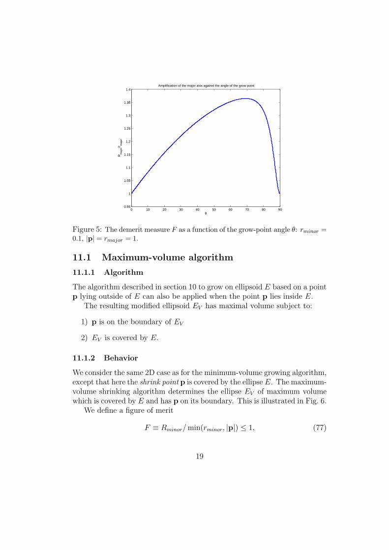
2. As illustrated in Fig. 5, for given E, F has a unique maximum (Fmax)at θ = θmax between θ = 0 and θ = π/2.
17
−1.5 −1 −0.5 0 0.5 1 1.5
−1
−0.5
0
0.5
1
Minimum−volume growing for grow point at 70 degrees
Figure 4: Illustration of the minimum-volume algorithm. The initial ellipse E(solid blue line); its bounding circle (dashed blue line); the grow point p (magenta);and the grown ellipse (red line) E: rminor = 0.1, |p| = rmajor = 1, θ = 70o.
3. As rminor decreases, θmax tends towards π/2, and Fmax tends towards√2.
With some justification, it is speculated that even in higher dimensionsF is bounded above by
√2.
11 Shrink E based on a given point
Given an ellipsoid E and a point p, the problem considered is to generate aconcentric ellipsoid E ′ of smaller volume which covers p. There is no uniquesolution to this problem. In the following three subsections we describe threealgorithms which yield different solutions for E ′, denoted by EV , EN and EC ,respectively.
The third (which is based on the first two) is preferred in application toISAT. The three algorithms are implemented in the routine ell pt shrink withthe parameter k ell set to 1, 2 and 3, respectively.
18
0 10 20 30 40 50 60 70 80 900.95
1
1.05
1.1
1.15
1.2
1.25
1.3
1.35
1.4
θ
Rm
ajor
/rm
ajor
Amplification of the major axis against the angle of the grow point
Figure 5: The demerit measure F as a function of the grow-point angle θ: rminor =0.1, |p| = rmajor = 1.
11.1 Maximum-volume algorithm
11.1.1 Algorithm
The algorithm described in section 10 to grow on ellipsoid E based on a pointp lying outside of E can also be applied when the point p lies inside E.
The resulting modified ellipsoid EV has maximal volume subject to:
1) p is on the boundary of EV
2) EV is covered by E.
11.1.2 Behavior
We consider the same 2D case as for the minimum-volume growing algorithm,except that here the shrink point p is covered by the ellipse E. The maximum-volume shrinking algorithm determines the ellipse EV of maximum volumewhich is covered by E and has p on its boundary. This is illustrated in Fig. 6.
We define a figure of merit
F ≡ Rminor/ min(rminor, |p|) ≤ 1, (77)
19
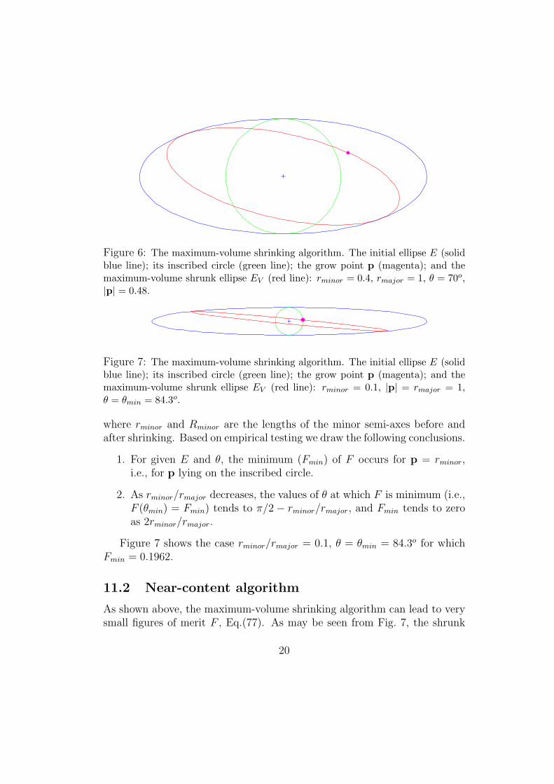
Figure 6: The maximum-volume shrinking algorithm. The initial ellipse E (solidblue line); its inscribed circle (green line); the grow point p (magenta); and themaximum-volume shrunk ellipse EV (red line): rminor = 0.4, rmajor = 1, θ = 70o,|p| = 0.48.
Figure 7: The maximum-volume shrinking algorithm. The initial ellipse E (solidblue line); its inscribed circle (green line); the grow point p (magenta); and themaximum-volume shrunk ellipse EV (red line): rminor = 0.1, |p| = rmajor = 1,θ = θmin = 84.3o.
where rminor and Rminor are the lengths of the minor semi-axes before andafter shrinking. Based on empirical testing we draw the following conclusions.
1. For given E and θ, the minimum (Fmin) of F occurs for p = rminor,i.e., for p lying on the inscribed circle.
2. As rminor/rmajor decreases, the values of θ at which F is minimum (i.e.,F (θmin) = Fmin) tends to π/2 − rminor/rmajor, and Fmin tends to zeroas 2rminor/rmajor.
Figure 7 shows the case rminor/rmajor = 0.1, θ = θmin = 84.3o for whichFmin = 0.1962.
11.2 Near-content algorithm
As shown above, the maximum-volume shrinking algorithm can lead to verysmall figures of merit F , Eq.(77). As may be seen from Fig. 7, the shrunk
20
ellipsoid can exclude a substantial portion of the original ellipsoid which iscloser to the center than the shrink point. Here we describe the alternative“near-content shrinking algorithm” which yields values of F of one, or closeto one. However, unlike the maximum-volume algorithm, the result dependson the metric of the space. It is implemented in the routine ell pt shrink (forthe parameter value k ell= 2).
11.2.1 Algorithm
We first describe the algorithm and then give its partial justification.The initial ellipsoid E centered at c is given in terms of the matrix A with
SVD A = UΣ2UT . We transform to principal axes (y-space) by defining
y = UTx, (78)
andp = UT (p− c). (79)
In y-space, the modified ellipsoid EN is defined as the rank-one modificationto E:
EN = {y |yTFy ≤ 1}, (80)
F = Σ2 + ρwwT , (81)
w = Dp, (82)
where the diagonal matrix D is defined by
Dii = max(0, 1/|p|2 − Σ2ii), (83)
and the positive scalar ρ is determined by the intersection condition
pTFp = 1. (84)
We make the following observations about the algorithm:
1. The quantity 1/|p|2−Σ2ii (appearing in Eq.(83)) is positive if, and only
if, the length of the i-th principal semi-axis Σ−1ii is greater than |p|.
21
2. Since E covers p, pTDp is strictly positive, and hence a positive valueof ρ exists which satisfies Eq.(84), namely
ρ = (1− pTΣ2p)/(pTDp). (85)
3. If p lies inside the ball of radius Σ−111 , then Dii = 1/|p|2 − Σ2
ii, p is aneigenvector of F, and hence p is the smallest principal semi-axis of EN .This is a necessary condition for EN to be a maximum nearest contentellipsoid.
4. If for some i (1 ≤ i < n), p lies between the balls of radius Σ−1ii
and Σ−1(i+1)(i+1), then wj = 0 for j ≤ i, and as a consequence the first
i principal axes of EN are the same as those of E. This again is anecessary condition for EN to be a maximum nearest content ellipsoid.
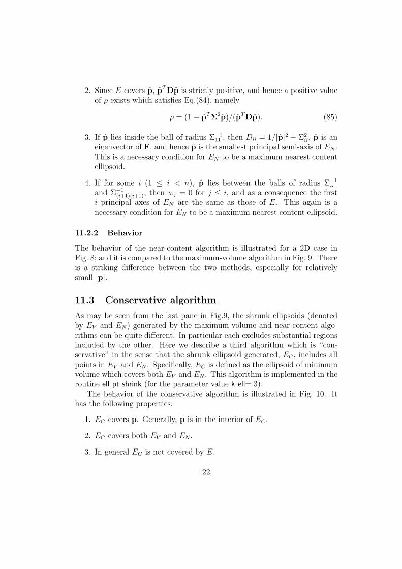
11.2.2 Behavior
The behavior of the near-content algorithm is illustrated for a 2D case inFig. 8; and it is compared to the maximum-volume algorithm in Fig. 9. Thereis a striking difference between the two methods, especially for relativelysmall |p|.
11.3 Conservative algorithm
As may be seen from the last pane in Fig.9, the shrunk ellipsoids (denotedby EV and EN) generated by the maximum-volume and near-content algo-rithms can be quite different. In particular each excludes substantial regionsincluded by the other. Here we describe a third algorithm which is “con-servative” in the sense that the shrunk ellipsoid generated, EC , includes allpoints in EV and EN . Specifically, EC is defined as the ellipsoid of minimumvolume which covers both EV and EN . This algorithm is implemented in theroutine ell pt shrink (for the parameter value k ell= 3).
The behavior of the conservative algorithm is illustrated in Fig. 10. Ithas the following properties:
1. EC covers p. Generally, p is in the interior of EC .
2. EC covers both EV and EN .
3. In general EC is not covered by E.
22
−1 −0.5 0 0.5 1
−0.5
0
0.5
Max. close content: |p|/rmin
=1.5
−1 −0.5 0 0.5 1
−0.5
0
0.5
Max. close content: |p|/rmin
=1.01
−1 −0.5 0 0.5 1
−0.5
0
0.5
Max. close content: |p|/rmin
=0.99
−1 −0.5 0 0.5 1
−0.5
0
0.5
Max. close content: |p|/rmin
=0.5
Figure 8: The near-content shrinking algorithm. The initial ellipse E (solid blueline); its inscribed circle (light blue line); the grow point p (magenta); and themaximum near content shrunk ellipse EN (red line): rmajor = 1, rminor = 0.4,θ = 70o.
4. The largest principal axis of EC can exceed that of E. Tests suggestthat this ratio of principal axes is seldom greater than 1.3.
5. The volume of EC is no greater than that of E, and in general is less.(This follows from the fact that both E and EC cover EV and EN , butEC is, by definition, of minimum volume.)
6. If the algorithm is applied a second time to EC based on the originalpoint p, the results is (in general) a different ellipsoid. (This is incontrast to the maximum-volume and near-content algorithms in whichp intersects the boundaries of EV and EN and hence a re-applicationof the algorithm has no effect.)
7. Because the algorithm involves EN , the result EC depends on the metricof the space.
23
−1 −0.5 0 0.5 1
−0.5
0
0.5
Max. close content: |p|/rmin
=1.6
−1 −0.5 0 0.5 1
−0.5
0
0.5
Max. close content: |p|/rmin
=1.2
−1 −0.5 0 0.5 1
−0.5
0
0.5
Max. close content: |p|/rmin
=0.6
−1 −0.5 0 0.5 1
−0.5
0
0.5
Max. close content: |p|/rmin
=0.2
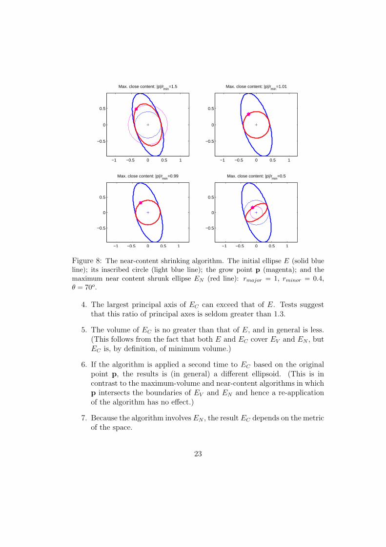
Figure 9: Comparison of the near-content and maximum-volume shrinking algo-rithms. The initial ellipse E (solid blue line); its inscribed circle (light blue line);the grow point p (magenta); the near content shrunk ellipse EN (red line); andthe maximum-volume shrunk ellipse EV (green line): rmajor = 1, rminor = 0.4,θ = 70o.
8. Tests reveal that the figure of merit F Eq.(77) is never less than unity.
The algorithm to generate EC consists of reducing the problem to twodimensions, and then solving a 2D problem. These two parts of the algorithmare described in the following two subsections.
11.3.1 Algorithm: reduction to 2D
Following the development in Sec. 11.2, we transform to the principal axesof E (y-space), defining y, p and w by Eq.(78), Eq.(79) and Eq.(82). ThenEN is defined by
EN = {y |yTFy ≤ 1}, (86)
withF = Σ2 + ρwwT . (87)
24
−1 −0.5 0 0.5 1
−0.5
0
0.5
Max. close content: |p|/rmin
=1.6
−1 −0.5 0 0.5 1
−0.5
0
0.5
Max. close content: |p|/rmin
=1.2
−1 −0.5 0 0.5 1
−0.5
0
0.5
Max. close content: |p|/rmin
=0.6
−1 −0.5 0 0.5 1
−0.5
0
0.5
Max. close content: |p|/rmin
=0.2
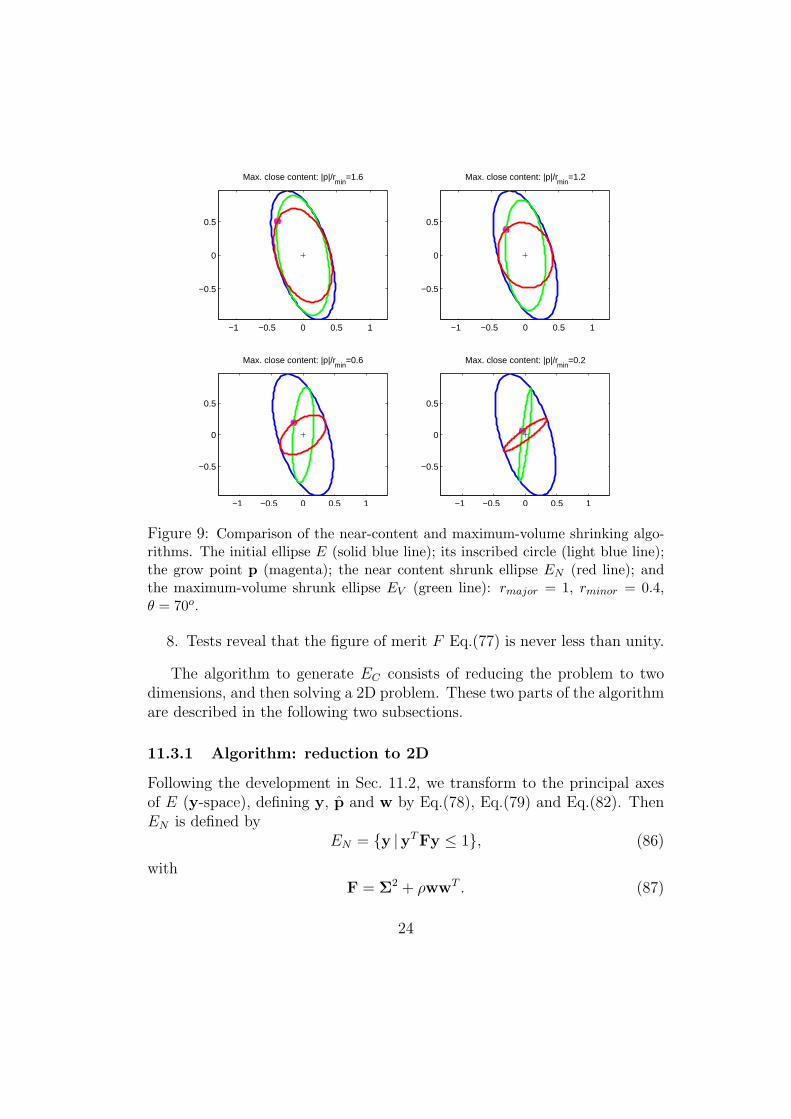
Figure 10: Conservative shrinking algorithm. The initial ellipse E (solid blue line);the grow point p (magenta); the maximum-volume shrunk ellipse, EV , (green line);the near-content shrunk ellipse, EN , (red line); and the conservative shrunk ellipse,EC , (magenta): rmajor = 1, rminor = 0.4, θ = 70o.
We now transform to z-space in which E is the unit ball:
z = Σy = ΣUTx. (88)
In z-space the definition of EN , Eq.(86), becomes
EN = {z | zT (I + ρww)z ≤ 1}, (89)
withw = Σ−1w. (90)
And the maximum volume shrunk ellipsoid is
EV = {z | zT (I + γppT )z ≤ 1}, (91)
where p is the transform of p
25
EN
E
1
1
−1
p
z2
z1−1
χ
EC
EV
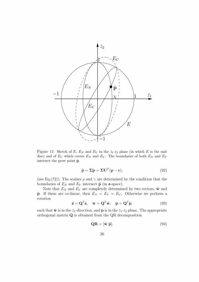
Figure 11: Sketch of E, EN and EV in the z1-z2 plane (in which E is the unitdisc) and of EC which covers EN and EV . The boundaries of both EN and EV
intersect the grow point p.
p = Σp = ΣUT (p− c), (92)
(see Eq.(72)). The scalars ρ and γ are determined by the condition that theboundaries of EN and EV intersect p (in z-space).
Note that EN and EV are completely determined by two vectors, w andp. If these are co-linear, then EN = EV = EC . Otherwise we perform arotation
z = QTz, w = QT w, p = QT p, (93)
such that w is in the z1-direction, and p is in the z1-z2 plane. The appropriateorthogonal matrix Q is obtained from the QR decomposition
QR = [w p]. (94)
26
Figure 11 is a sketch of the intersection of the ellipsoids with the z1-z2
plane. Note that in the other directions the principal semi-axes are unitvectors aligned with the coordinate axes. The minimum volume ellipsoid EC
covering EN and EV is also shown in the figure. Its intersection with thez1-z2 plane is given by the ellipse
E ′C = {(z1, z2) | ‖LT
[z1
z2
]‖ ≤ 1}, (95)
where L is a 2×2 Cholesky matrix which is determined in the next subsection.Thus the ellipsoid EC is given by
EC = {z | ‖LTz‖ ≤ 1}, (96)
where the n× n Cholesky matrix L is
L =
[L 00 I
]. (97)
Transforming Eq.(96) back to the original x-space, we obtain
EC = {x | ‖LTC(x− c)|| ≤ 1}, (98)
where the Cholesky matrix LC is obtained from
AC = LCLTC = BCBT
C , (99)
BC = UΣQL. (100)
11.3.2 Algorithm: solution in 2D
The problem to be solved is the determination of the 2× 2 Cholesky matrixL defining the covering ellipse EC in the z1-z2 plane (see Fig. 11).
The scalars ρ and γ in Eq.(89) and Eq.(91) are determined by the inter-section condition (of ∂EN and ∂EV with p) to be
ρ = (1− |p|2)/p21, (101)
27
γ = (1− p|2)/|p|4, (102)
and the intersection of EN with the z1 axis is at z1 = χ
χ =|p1|√1− p2
2
. (103)
A transformation to ζ-space is performed
[ζ1
ζ2
]= C
[z1
z2
]=
[1/χ 00 1
] [z1
z2
], (104)
consisting of a stretching in the z1 direction so that EN transforms to theunit disc.
With this transformation EV becomes
EV = {ζ | ζT Aζ ≤ 1}, (105)
with
A =
[a cc b
]=
[χ2(1 + γp2
1) γχp1p2
γχp1p2 1 + γp22
]. (106)
The SVD of A isA = UΣ
2UT , (107)
with
U =
[cos θ sin θ− sin θ cos θ
], (108)
θ = 12tan−1(−2c/(a− b)), (109)
Σ211 = a cos2 θ − 2c sin θ cos θ + b sin2 θ, (110)
Σ222 = a sin2 θ + 2c sin θ cos θ + b cos2 θ. (111)
Now EC is the ellipse which covers EN (which is the unit disc) and EV
which has principal semi-axes whose directions are given by the columns ofU and whose lengths are Σ−1
11 and Σ−122 . (In general, one of Σ11 and Σ22 is
less than unity and one greater than unity.) Thus the covering ellipse EC
has the same principal directions
28
EC = {ζ | ζT UΣ2UT ζ ≤ 1}, (112)
and eigenvaluesΣ11 = min(1, Σ11), (113)
Σ22 = min(1, Σ22). (114)
Transforming back to z1-z2 we obtain the required result that EC is givenby Eq.(95), where the 2× 2 Cholesky matrix L is obtained as
LLT
= CUΣ2U
TC. (115)
12 Orthogonal projection of E onto a given
line
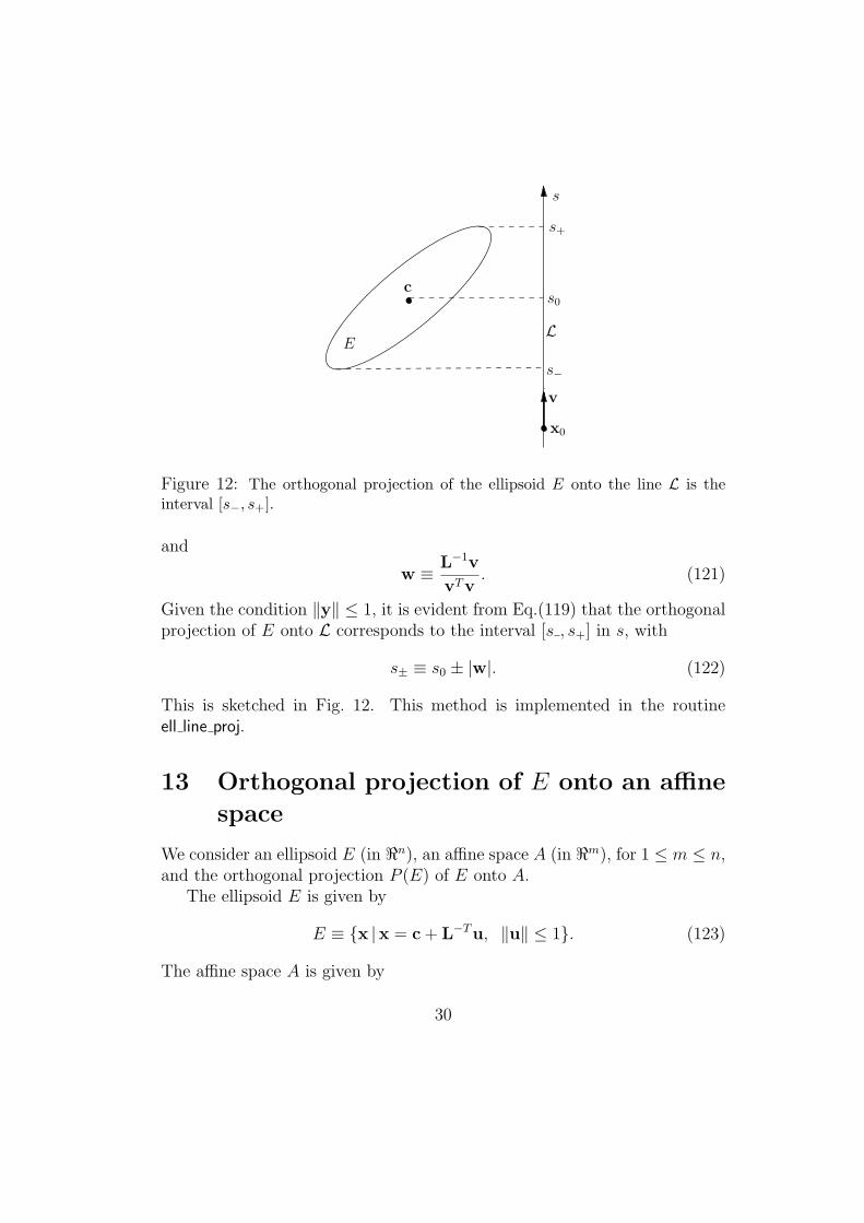
We consider a given line L, parameterized by s, defined by
L ≡ {x |x = x0 + sv}, (116)
where x0 is a given point and v is a given non-zero vector, see Fig. 12. Givenany point x in the space, its orthogonal projection onto L corresponds to
s =vT (x− x0)
vTv. (117)
Now the given ellipsoid E is given by
E = {x |x = c + L−Ty, ||y|| ≤ 1}. (118)
Thus the projection of points in E correspond to values of s
s =vT (L−Ty + c− x0)
vTv= s0 + wTy, for ‖y‖ ≤ 1, (119)
where
s0 ≡ vT (c− x0)
vTv, (120)
29
E
x0
v
s−
s0
s+
s
L
c
Figure 12: The orthogonal projection of the ellipsoid E onto the line L is theinterval [s−, s+].
and
w ≡ L−1v
vTv. (121)
Given the condition ‖y‖ ≤ 1, it is evident from Eq.(119) that the orthogonalprojection of E onto L corresponds to the interval [s , s+] in s, with
s± ≡ s0 ± |w|. (122)
This is sketched in Fig. 12. This method is implemented in the routineell line proj.
13 Orthogonal projection of E onto an affine
space
We consider an ellipsoid E (in <n), an affine space A (in <m), for 1 ≤ m ≤ n,and the orthogonal projection P (E) of E onto A.
The ellipsoid E is given by
E ≡ {x |x = c + L−Tu, ‖u‖ ≤ 1}. (123)
The affine space A is given by
30
A ≡ {x |x = d + Tt}, (124)
where d is a given m-vector, T is a given n × m orthogonal matrix, and tis a vector of m parameters. The orthogonal projection of a general point xonto A is
P (x) = d + TTT (x− d). (125)
We thus obtain
P (E) = {x |x = d + TTT (c− d + L−Tu), ‖u‖ ≤ 1}. (126)
Now let the SVD of TTL−T be
TTL−T = U[Σ0]VT . (127)
ThenTTL−Tu = UΣw, (128)
where w denotes the first m elements of
w ≡ VTu. (129)
Note that ‖u‖ ≤ 1 implies ‖w‖ ≤ 1. Thus we obtain
P (E) = {x |x = d + T(c + UΣw), ‖w‖ ≤ 1}, (130)
wherec ≡ TT (c− d). (131)
The above equation for P (E) is for an m-dimensional ellipsoid in A. Itcan be put in standard form by defining B by
B−T = UΣ, (132)
and then L asLL
T= BBT , (133)
so that we can write
P (E) = {x |x = d + T(c + L−T
w), ‖w‖ ≤ 1}. (134)
The Cholesky matrix L can be computed from the LQ decomposition
UΣ−1 = LQ. (135)
This method is implemented in the routine ell aff pr.
31
14 Generate an ellipsoid which does not cover
any specified points
We are given a point c, a set of P points p(j)(j = 1 : P ) and a positive lengthrmax. The problem is to generate an ellipsoid E which
1. is centered at c
2. has principal semi-axes no larger than rmax
3. does not cover any of the P points
4. and is “as large as possible” (in an undefined sense).
The algorithm used to solve this problem is implemented in the routineell pts uncover. It involves a user-specified parameter θ (0 < θ ≤ 1) whichaffects the shape of the resulting ellipsoid, E.
The algorithm has two phases. In the first phase there are n stages whichgenerate a succession of ellipsoids E1, E2, . . ., En. In the second phase, E isformed by shrinking En uniformly and minimally so that none of the pointsis covered.
In the first phase, a principle axis is determined on each stage. The ellip-soid Ek is determined on the kth stage, and it has the following properties:
1. Ek is centered at c
2. for 1 ≤ ` < k, the `th principle axis of Ek is the same as that of E`
(previously determined on stage `)
3. the kth principle axis (of half-length rk ≤ rmax) is determined on thekth stage
4. for k < ` ≤ n, the `th principle axis of Ek is of half-length rk.
Note that E1 is a ball of radius r1.An orthonormal basis is developed with basis vectors e1, e2, ..., en. On
the kth stage e` (` ≥ k) is modified, but subsequently ek is not altered. Atthe end of the kth stage, the basis vectors are principal axes of Ek. Thevectors y(j)(j = 1 : P ) store the coordinates of the points (relative to c) inthe current basis. For the jth particle we define
32
hj =n∑
i=1
(y(j)i /ri)
2. (136)
At the end of the kth stage (since r` = rk for ` ≥ k) we can decompose hj as
hj = fj + gj/r2k, (137)
where
fj =k−1∑
i=1
(y(j)i /ri)
2, (138)
and
gj =n∑
i=1
(y(j)i )2. (139)
The ellipsoid Ek does not cover the point j if hj is greater than unity. Thiscondition (hj > 1) can be re-expressed as
gj/r2k > (1− fj). (140)
Points with fj > 1 cannot be covered by Ek regardless of how large rk is.Such points are “excluded.” Points with
θ2 < fj ≤ 1, (141)
are “partially excluded.” Such points cannot be covered by Ek shrunk by afactor of θ. The remaining points (i.e., with fj ≤ θ2) are “included.”
We define r2k to be the minimum value over the included points of gj/(1−
fj), and denote by j the index of a point that achieves this minimum. Thesignificance of rk is that if rk is set to rk, then the point j is on the boundaryof Ek, but no points are in the interior of Ek. If rk is greater than rmax (or ifthere are no included points), then we get r` = rmax for all ` ≥ k, and omitthe remaining stages of the first phase. Otherwise rk is set to rk, and the
basis vectors e` (k ≤ ` ≤ n) are re-defined so that y(j)` = 0 for ` > k. In this
way, in subsequent stages, the ellipsoid can expand in directions orthogonalto y(j), with y(j) remaining on the boundary.
At the end of the first phase there are no included points, and En doesnot cover any excluded points. However En may cover one or more partiallyexcluded points. Consequently, the final result E is obtained by shrinking En
uniformly, as little as possible so that none of the partially included pointsis covered.
33
v
E1
E2
E ′
2
E ′
1
H ′
H
(b)(a)
xh
y2
yh
y1
O
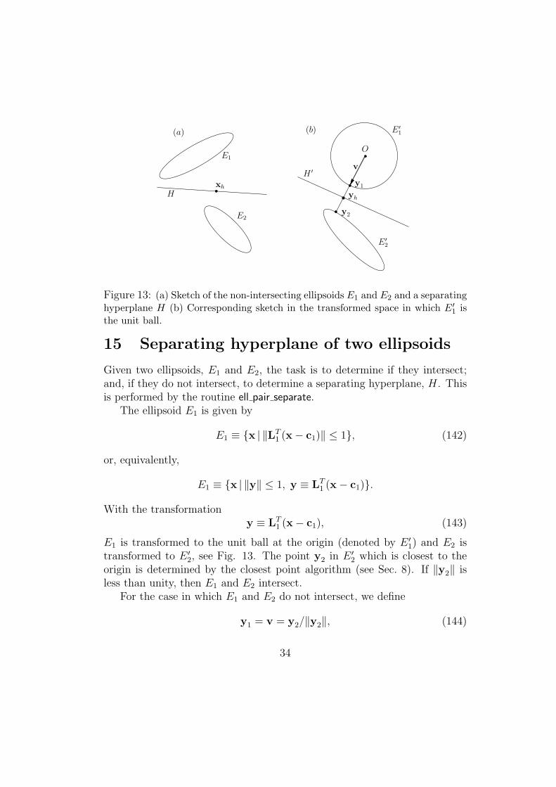
Figure 13: (a) Sketch of the non-intersecting ellipsoids E1 and E2 and a separatinghyperplane H (b) Corresponding sketch in the transformed space in which E′
1 isthe unit ball.
15 Separating hyperplane of two ellipsoids
Given two ellipsoids, E1 and E2, the task is to determine if they intersect;and, if they do not intersect, to determine a separating hyperplane, H. Thisis performed by the routine ell pair separate.
The ellipsoid E1 is given by
E1 ≡ {x | ‖LT1 (x− c1)‖ ≤ 1}, (142)
or, equivalently,
E1 ≡ {x | ‖y‖ ≤ 1, y ≡ LT1 (x− c1)}.
With the transformationy ≡ LT
1 (x− c1), (143)
E1 is transformed to the unit ball at the origin (denoted by E ′1) and E2 is
transformed to E ′2, see Fig. 13. The point y2 in E ′
2 which is closest to theorigin is determined by the closest point algorithm (see Sec. 8). If ‖y2‖ isless than unity, then E1 and E2 intersect.
For the case in which E1 and E2 do not intersect, we define
y1 = v = y2/‖y2‖, (144)
34
so that y1 and y2 are the pair of closest points in E ′1 and E ′
2. Note that v isa unit vector. Then we define
yh ≡ 12(y1 + y2), (145)
and a separating hyperplane is defined by
H ′ ≡ {y |vT (y − yh) = 0}. (146)
Inverting the transformation Eq.(143), we obtain the separating hyper-plane in the original space:
H ≡ {x |uT (x− xh) = 0}, (147)
where
u =L1v
‖L1v‖ , (148)
andxh = c1 + L−T
1 yh. (149)
For a hyperplane H given by Eq.(147) (for some u and xh), we define thequality q as follows. Let x1 be the point in E1 closest to H, and similarly letx2 be the point in E2 closest to H. The quality q is defined as
q ≡ uT (x2 − x1)
|x2 − x1| ≤ 1. (150)
This is the distance between the supporting hyperplanes at x1 and x2 relativeto their separation. The maximum possible distance between the supportinghyperplanes is achieved for q = 1, and this occurs when x1 and x2 are themutually closest points in E1 and E2.
In the routine ell pair separate there is an option to iteratively improvethe quality of the hyperplane. Initially x1 and x2 are set to the points in E1
and E2 corresponding to y1 and y2 (in E ′1 and E ′
2). Then, successively, x1
is replaced by the closest point in E1 to x2; and then x2is replaced by theclosest point in E2 to x1. The hyperplane is then taken as the perpendicularbisector of the line x1 − x2. It is not guaranteed that this hyperplane isseparating, nor that the quality increases with the iterations, although itgenerally does. Consequently, H is taken as the hyperplane with the greatestquality encountered initially or during the iterations.
35
(Note that the separating hyperplane of quality q = 1 could alternativelybe obtained by solving the quadratic programming problem, of determiningthe mutually closest points x1 and x2 in E1 and E2. This has not beenimplemented.)
16 Pair covering query
Given a pair of ellipsoids E1 and E2 (centered at c1 and c2 and with Choleskyfactors L1 and L2), the problem is to determine whether E1 covers E2. Thisquery is answered by the routine ell pair cover query by the following algo-rithm.
With the same transformation as used in Sec. 15, E1 is transformed tothe unit ball, at the origin, and E2 to E ′
2 (see Eq.(143) and Fig.13). Thealgorithm described in Sec. 9 is then used to determine the distance s fromthe origin to the furthest point in E ′
2. The ellipsoid E1 covers E2 if and onlyif s is less than or equal to unity.
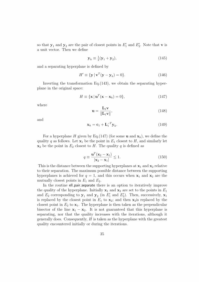
17 Shrink ellipsoid so that it is covered by a
concentric ellipsoid
Given two concentric ellipsoids, E1, and E2, the task is to form the maximal-volume ellipsoid, E, which is covered by both E1 and E2. This is performedby the routine ell pair shrink.
Clearly E is concentric with E1 and E2, and so, without loss of generality,we take the origin at the mutual center. Then, E1 is given by
E1 ≡ {x | ‖LT1 x‖ ≤ 1}, (151)
and similarly for E2 and E (in terms of L2 and L, respectively).The transformation
y = LT1 x, (152)
maps E1 to the unit ball, E ′1, and it maps E2 to the ellipsoid E ′
2 with Choleskyfactor
L′2 = L−11 L2, (153)
see Fig. 14. Note that E ′1 shares the principal axes of E ′
2. Hence E ′ (i.e.,the mapped covered ellipsoid E) has the same principal directions as E ′
2; and
36
E
(b)(a)
E1
E′
2
E2
E′
E′
1
Figure 14: (a) Sketch of the concentric ellipsoids E1 and E2 and the maximal-volume ellipsoid E which is covered by them (b) Corresponding ellipsoids in thetransformed space in which E′
1 is the unit ball.
the lengths of its principal axes are the lesser of those of E ′1 (all of which are
unity) and those of E ′2. Thus if
L′2 = UΣVT , (154)
is the SVD of L′2, so that
L′2L′T2 = UΣ2UT , (155)
then the Cholesky matrix of E ′ is given by
L′L′T = UΣ2UT , (156)
where the singular values Σii = σi are given by
σi = max(σi, 1), (157)
where σi ≡ Σii.The Cholesky matrix of E is obtained by inverting the transformation:
L = L1L′. (158)
The same algorithm can be used to determine the minimal-volume el-lipsoid which covers E1 and E2. In that case, in contrast to Eq.(157), theappropriate singular values are:
σi = min(σi, 1). (159)
37
18 Ellipsoid that covers two given ellipsoids
Given two ellipsoids E1 and E2, the task is to determine a third ellipsoid Ethat covers both E1 and E2. Ideally E is of minimal volume.
It is a problem of convex optimization to determine the minimum-volumecovering ellipsoid (see, e.g., Boyd and Vandenberghe 2004). An algorithm isprovided by Yildirim (2006). It appears that the solution to this convexoptimization problem is computationally expensive. Instead, in the subsec-tions, we describe heuristic algorithms with determine ellipsoids E (not ofminimal volume) which cover E1 and E2. These methods are implementedin the routine ell pair cover, with the parameter algorithm determining theparticular algorithm to be used.
18.1 Spheroid algorithm
The ellipsoids E1 and E2 have centers c1 and c2, and outer radii rout,1 androut,2. Thus the ball B1 centered at c1 of radius rout,1 covers E1, and similarlywe define the ball B2 which covers E2. In this “spheroid algorithm” (algorithm= 1) we take E to be the minimum-volume ball B which covers B1 and B2.
The center and radius of B are determined as follows. Consider the lineof centers with distance s measured from c1 towards c2. Let the distancebetween the centers be ∆c ≡| c2− c1 |. There are four intersections betweenthe ball B1 and B2 and the line. The outermost of these corresponds to
smax = max(rout,1, ∆c + rout,2), (160)
and
smin = min(−rout,1, ∆c− rout,2). (161)
Thus the center of B is
c = c1 +1
2(smin + smax)(c2 − c1)/∆c, (162)
and its radius is
r =1
2(smax − smin). (163)
38
A variant is the “spheroid algorithm with shrinking” (algorithm = 4), inwhich r is decreased to r′ to yield the ball B′ of minimum volume centered atc which covers E1 and E2. The radius r′ is determined as the greatest distancefrom c to any point in E1 and E2 (which is determined by ell pt near far).
18.2 Covariance algorithm
The ellipsoid E1 is defined by
E1 ≡ {x | (x− c1)TA1(x− c1) ≤ 1}, (164)
and E2 and E are similarly defined by c2 and A2, and by c and A, respec-tively.
In the “covariance” algorithm described in this section, we define thecovering ellipsoid E by
c ≡ 12(c1 + c2), (165)
A ≡ αA0, (166)
andA0 ≡
(A−1
1 + A−12 + 1
4[c1 − c2][c1 − c2]
T)−1
, (167)
where α is a positive parameter to be determined.To determine α, we consider the ellipsoid E0 defined by c and A0. With
L0 being the Cholesky factor
L0LT0 = A0, (168)
we perform the linear transformation
y = c + L−T0 x. (169)
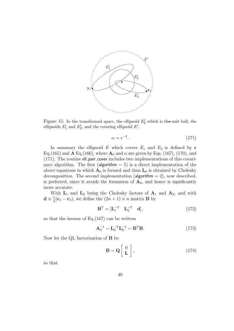
As depicted in Fig. 15, this transforms E0 to the unit ball, and E1 and E2
to ellipsoids denoted by E ′1 and E ′
2.Using the furthest-point algorithm (see Sec. 9), we determine y1 and y2,
defined as the points on E ′1 and E ′
2, respectively, which are furthest from theorigin (see Fig. 15). Clearly, the ball E ′ of radius
r ≡ max(‖y1‖, ‖y2‖) (170)
covers E ′1 and E ′
2. This corresponds to E ′ (the transformation of E) with
39
y2
E′
0
E′
E′
1
y1
E′
2
Figure 15: In the transformed space, the ellipsoid E′0 which is the unit ball, the
ellipsoids E′1 and E′
2, and the covering ellipsoid E′.
α = r−2. (171)
In summary the ellipsoid E which covers E1 and E2 is defined by cEq.(165) and A Eq.(166), where A0 and α are given by Eqs. (167), (170), and(171). The routine ell pair cover includes two implementations of this covari-ance algorithm. The first (algorithm = 5) is a direct implementation of theabove equations in which A0 is formed and then L0 is obtained by Choleskydecomposition. The second implementation (algorithm = 2), now described,is preferred, since it avoids the formation of A0, and hence is significantlymore accurate.
With L1 and L2 being the Cholesky factors of A1 and A2, and withd ≡ 1
2(c1 − c2), we define the (2n + 1)× n matrix B by
BT = [L−T1 L−T
2 d], (172)
so that the inverse of Eq.(167) can be written
A−10 = L−T
0 L−10 = BTB. (173)
Now let the QL factorization of B be
B = Q
[0L
], (174)
so that
40
BTB = LTL. (175)
By comparing the above two equations, we see that L0 is the inverse ofL. Thus, in this preferred QL implementation of the covariance algorithm,the Cholesky matrix L0 required in Eq.(169) is obtained as L−1, where L isobtained from the QL factorization of B, defined by Eq.(172).
18.3 Iterative algorithm
The algorithm described here (which is also implemented in the routineell pair cover with algorithm= 2), is more elaborate and expensive than the“covariance” algorithm described in the previous subsection, but in mostcircumstances it generates a covering ellipsoid E of smaller volume.
Given E1 and E2, the algorithm proceeds through six stages (describedbelow) to generate the covering ellipsoid E. Stages 1, 2 and 6 are trivial,but are retained for consistency with the implementation in ell pair cover. InStages 3 and 4 the shape of E (but not its center and size) are determined.The center of E is taken to be on the line of centers of E1 and E2. Its locationis determined iteratively in Stage 5 so as to minimize the volume of E.
Various spaces are considered, and are referred to as x-space, y-space,z-space and ζ-space. The ellipsoids E1 and E2 are given in x-space, and thecovering ellipsoid E is to be determined in this space. The other spaces areobtained by successive linear transformations; and E2(z), for example, de-notes the ellipsoid E2 viewed in z-space, which has center c2(z) and Choleskytriangle L2(z).
18.3.1 Stage 1
The two ellipsoids E1 and E2 are given in x-space (in terms of c1, L1, c2 andL2): see Fig.16(a).
18.3.2 Stage 2
We denote by E01 and E0
2 the two given ellipsoids shifted to the origin: seeFig.16(b). (In general, E0
m denotes Em shifted to the origin.)
18.3.3 Stage 3
The transformed variable y is defined by
41
E0
2
E1
E2
c1
(a)
c2
O
(b) E0
1
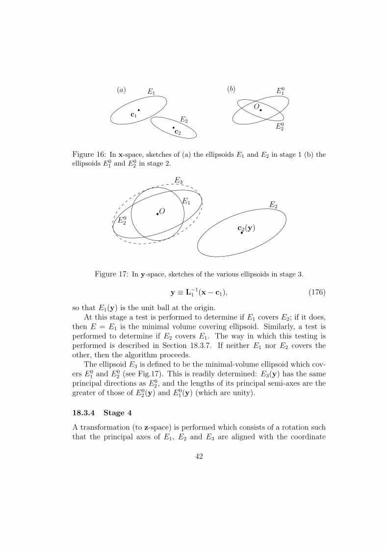
Figure 16: In x-space, sketches of (a) the ellipsoids E1 and E2 in stage 1 (b) theellipsoids E0
1 and E02 in stage 2.
E0
2
E2
E3
E1
O
c2(y)
Figure 17: In y-space, sketches of the various ellipsoids in stage 3.
y ≡ L−11 (x− c1), (176)
so that E1(y) is the unit ball at the origin.At this stage a test is performed to determine if E1 covers E2; if it does,
then E = E1 is the minimal volume covering ellipsoid. Similarly, a test isperformed to determine if E2 covers E1. The way in which this testing isperformed is described in Section 18.3.7. If neither E1 nor E2 covers theother, then the algorithm proceeds.
The ellipsoid E3 is defined to be the minimal-volume ellipsoid which cov-ers E0
1 and E02 (see Fig.17). This is readily determined: E3(y) has the same
principal directions as E02 , and the lengths of its principal semi-axes are the
greater of those of E02(y) and E0
1(y) (which are unity).
18.3.4 Stage 4
A transformation (to z-space) is performed which consists of a rotation suchthat the principal axes of E1, E2 and E3 are aligned with the coordinate
42
E4
E3 = B1
E1
w
smin
L
B2
smax
E2
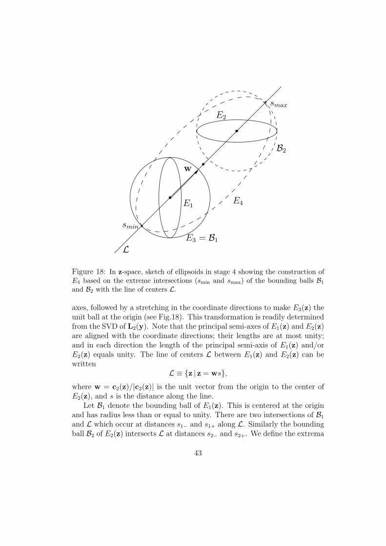
Figure 18: In z-space, sketch of ellipsoids in stage 4 showing the construction ofE4 based on the extreme intersections (smin and smax) of the bounding balls B1
and B2 with the line of centers L.
axes, followed by a stretching in the coordinate directions to make E3(z) theunit ball at the origin (see Fig.18). This transformation is readily determinedfrom the SVD of L2(y). Note that the principal semi-axes of E1(z) and E2(z)are aligned with the coordinate directions; their lengths are at most unity;and in each direction the length of the principal semi-axis of E1(z) and/orE2(z) equals unity. The line of centers L between E1(z) and E2(z) can bewritten
L ≡ {z | z = ws},where w = c2(z)/|c2(z)| is the unit vector from the origin to the center ofE2(z), and s is the distance along the line.
Let B1 denote the bounding ball of E1(z). This is centered at the originand has radius less than or equal to unity. There are two intersections of B1
and L which occur at distances s1− and s1+ along L. Similarly the boundingball B2 of E2(z) intersects L at distances s2− and s2+. We define the extrema
43

of these intersections by
smin ≡ min(s1−, s1+, s2−, s2+), (177)
andsmax ≡ max(s1−, s1+, s2−, s2+). (178)
The ellipsoid E4 is now defined to be centered at
s0 ≡ 12(smin + smax), (179)
to have a principal semi-axis of length 12(smax− smin) in the direction w, and
to have all other principal axes unity. In other words, E4(z) is formed fromthe unit ball at s0 by stretching it in the ±w directions so that it intersectsthe extrema smin and smax.
18.3.5 Stage 5
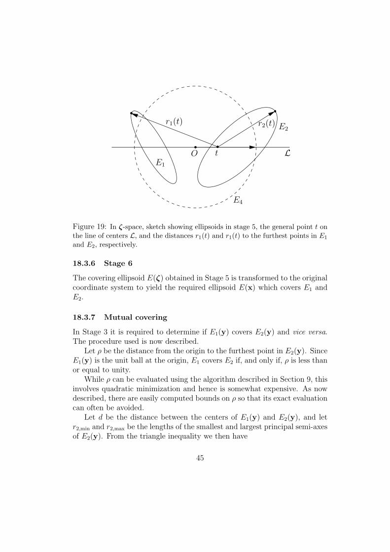
A transformation is performed to ζ-space such that E4(ζ) is the unit ball atthe origin, and the line of centers L(ζ) is in the first coordinate direction:
L(ζ) = {ζ | ζi = tδi1}, (180)
where t measures the distance along the line (see Fig.19).The covering ellipsoid being constructed E(ζ) is a ball of radius r0 cen-
tered at a distance t0 along L. It remains to determine r0 and t0.Consider a ball centered at a distance t along L. Let r1(t) denote the
distance from the ball’s center to the furthest point in E1(ζ). This canbe determined by the algorithm described in Section 9. Similarly, let r2(t)denote the distance to the furthest point in E2(ζ); and we define
r(t) ≡ max(r1(t), r2(t)). (181)
Thus the ball centered at a distance t along L and of radius r(t) covers bothE1(ζ), and E2(ζ).
In the definition of E(ζ), we take t0 to be (an approximation to) the valueof t at which r(t) is minimum, and then define r0 ≡ r(t0)
As one moves along the line L from the center of E1(ζ) to the centerof E2(ζ), r1(t) continually increases and r2(t) continually decreases. Exceptin unusual circumstances, the minimum of r(t) occurs between the centers,where r1(t) equals r2(t). A simple iterative procedure usually determines thelocation of the minimum (to reasonable accuracy) in two or three iterations.
44
O
E2
E1
r2(t)
E4
L
r1(t)
t
Figure 19: In ζ-space, sketch showing ellipsoids in stage 5, the general point t onthe line of centers L, and the distances r1(t) and r1(t) to the furthest points in E1
and E2, respectively.
18.3.6 Stage 6
The covering ellipsoid E(ζ) obtained in Stage 5 is transformed to the originalcoordinate system to yield the required ellipsoid E(x) which covers E1 andE2.
18.3.7 Mutual covering
In Stage 3 it is required to determine if E1(y) covers E2(y) and vice versa.The procedure used is now described.
Let ρ be the distance from the origin to the furthest point in E2(y). SinceE1(y) is the unit ball at the origin, E1 covers E2 if, and only if, ρ is less thanor equal to unity.
While ρ can be evaluated using the algorithm described in Section 9, thisinvolves quadratic minimization and hence is somewhat expensive. As nowdescribed, there are easily computed bounds on ρ so that its exact evaluationcan often be avoided.
Let d be the distance between the centers of E1(y) and E2(y), and letr2,min and r2,max be the lengths of the smallest and largest principal semi-axesof E2(y). From the triangle inequality we then have
45
ρ ≤ d + r2,max, (182)
andρ ≥ d + r2,min. (183)
We also haveρ ≥ r2,max. (184)
Thus, if d + r2,max ≤ 1, then ρ ≤ 1, and so E1 covers E2. On the other hand,if d + r2,min > 1 or r2,max > 1, then ρ > 1, and so E1 does not cover E2. Inthe remaining cases, E1 may cover E2, and so ρ is evaluated.
18.3.8 Discussion
While this algorithm is more elaborate and expensive than that given inSection 18.2, it generally yields a covering ellipsoid E of smaller volume. Inparticular it yields the ellipsoid of minimal volume if E1 and E2 are concentricor if one covers the other.
The principal computational expenses are:
1. The SVD of L2(y) performed in Stage 3
2. The quadratic minimization involved in the furthest-point algorithm(Section 9) which is invoked 0, 1 or 2 times (in Stage 3) to determineif E1 and E2 cover each other
3. The quadratic minimization involved in the furthest-point algorithmwhich is invoked twice per iteration (to evaluate r1(t) and r2(t)) inStage 5.
19 Conclusions
Algorithms have been described for performing some basic geometric opera-tions on ellipsoids. A Fortran implementation of these algorithms is providedby the Ell LIB library.
20 Acknowledgments
I am particularly grateful to Professor Charles Van Loan for his help onnumerous occasion with issues of numerical linear algebra.
46
References
Averick, B. M., R. Carter, and J. More (1993). MINPACK-2. http://www-fp.mcs.anl.gov/OTC/minpack/summary.html.
Boyd, S. and L. Vandenberghe (2004). Convex Optimization. Cambridge:Cambridge University Press.
Golub, G. H. and C. F. Van Loan (1996). Matrix Computations (3rd ed.).Baltimore: Johns Hopkins University Press.
Pope, S. B. (1997). Computationally efficient implementation of combus-tion chemistry using in situ adaptive tabulation. Combust. TheoryModelling 1, 41–63.
Yildirim, E. A. (2006). On the minimum volume covering ellipsoid of el-lipsoids. SIAM Journal on Optimization 17, 621–641.
47