www.sciencemag.org/cgi/content/full/321/5887/385/DC1

Supporting Online Material for

Measurement of the Elastic Properties and Intrinsic Strength of Monolayer Graphene

Changgu Lee, Xiaoding Wei, Jeffrey W. Kysar, James Hone*

*To whom correspondence should be sent. E-mail: jh2228@columbia.edu

Published 18 July 2008, Science 321, 385 (2008)

DOI: 10.1126/science.1157996

This PDF file includes:

Materials and Methods Figs. S1 to S8 References

Measurement of the Elastic Properties and Intrinsic Strength of Monolayer Graphene

Changgu Lee1,2, Xiaoding Wei1, Jeffrey W. Kysar1,3, James Hone1,2,4,*

1Department of Mechanical Engineering

2DARPA Center for Integrated Micro/Nano-Electromechanical Transducers (iMINT) 3Center for Nanostructured Materials

4 Center for Electronic Transport in Molecular Nanostructures Columbia University New York, NY 10027

Materials and Methods Preparation of samples The substrate was fabricated using nanoimprint lithography and reactive ion etching (RIE). The nanoimprint master, consisting of a 5 × 5 mm array of circles (1 and 1.5 µm diameters), was fabricated by electron-beam lithography, and etched to a depth of 100 nm using RIE, and coated with an anti-adhesion agent (NXT-110, Nanonex). The sample wafer (Si with a 300 nm SiO2 epilayer) was coated with 10 nm Cr by thermal evaporation, followed by a 120 nm spin-coated PMMA layer. The imprint master was used to imprint the PMMA do a depth of 100 nm. The residual layer of the PMMA was etched in oxygen RIE, and the chromium layer was etched in a chromium etchant (Cr-7S, Cyantek) for 15 seconds. Using the chromium as an etch mask, fluorine-based RIE was used to etch through the oxide and into the silicon to a total depth of 500nm. The chromium layer was then removed.

Flake #2

Flake #1(I)

(II) (III)(A) (B)

Flake #2

Flake #1(I)

(II) (III)(A) (B)

Figure S1. Graphene layer identification using (a) optical microscopy; (b) Raman spectroscopy at 633 nm. The flakes marked I, II, and III contain one, two, and three atomic sheets, respectively.

Graphene was deposited by mechanical cleavage and exfoliation according to the method in (S1). A small piece of Kish graphite (Toshiba Ceramics) was laid on Scotch tape, and thinned by folding repeatedly. The thinned graphite was pushed down onto the patterned substrate, rubbed gently, and then detached. The deposited flakes were examined with an optical microscope to identify candidate graphene flakes with very few atomic layers. The number of graphene layers was confirmed using Raman spectroscopy (S2). Fig. S1A shows an optical image of graphene * Corresponding author. E-mail: jh2228@columbia.edu

- 1 -

layers and the Raman spectra of the graphene layers. Stolyarova et al. (S3) characterized the monolayer graphene flakes fabricated from the same graphite source by similar procedures with STM (Scanning Tunnelling Microscopy). Their results showed the graphene flake to be defect-free over an area of 100×100 nm2.

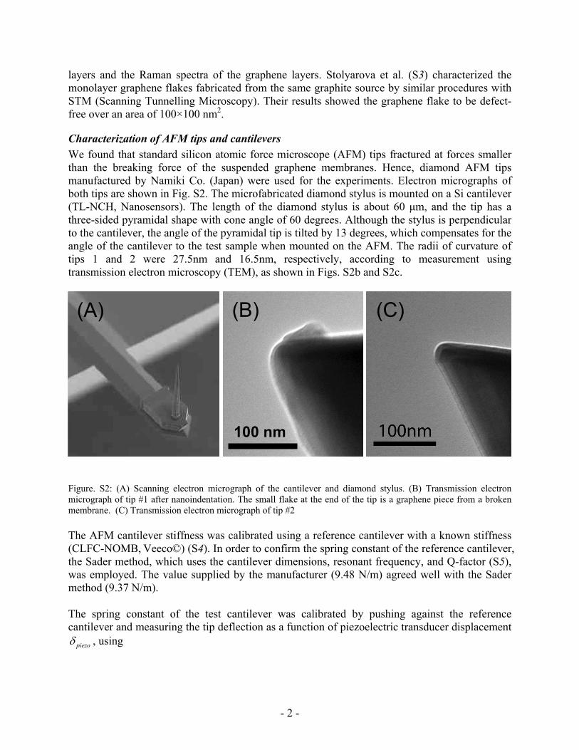
Characterization of AFM tips and cantilevers We found that standard silicon atomic force microscope (AFM) tips fractured at forces smaller than the breaking force of the suspended graphene membranes. Hence, diamond AFM tips manufactured by Namiki Co. (Japan) were used for the experiments. Electron micrographs of both tips are shown in Fig. S2. The microfabricated diamond stylus is mounted on a Si cantilever (TL-NCH, Nanosensors). The length of the diamond stylus is about 60 μm, and the tip has a three-sided pyramidal shape with cone angle of 60 degrees. Although the stylus is perpendicular to the cantilever, the angle of the pyramidal tip is tilted by 13 degrees, which compensates for the angle of the cantilever to the test sample when mounted on the AFM. The radii of curvature of tips 1 and 2 were 27.5nm and 16.5nm, respectively, according to measurement using transmission electron microscopy (TEM), as shown in Figs. S2b and S2c.

(B) (C)(A)

100 nm

Figure. S2: (A) Scanning electron micrograph of the cantilever and diamond stylus. (B) Transmission electron micrograph of tip #1 after nanoindentation. The small flake at the end of the tip is a graphene piece from a broken membrane. (C) Transmission electron micrograph of tip #2

The AFM cantilever stiffness was calibrated using a reference cantilever with a known stiffness (CLFC-NOMB, Veeco©) (S4). In order to confirm the spring constant of the reference cantilever, the Sader method, which uses the cantilever dimensions, resonant frequency, and Q-factor (S5), was employed. The value supplied by the manufacturer (9.48 N/m) agreed well with the Sader method (9.37 N/m). The spring constant of the test cantilever was calibrated by pushing against the reference cantilever and measuring the tip deflection as a function of piezoelectric transducer displacement

piezoδ , using

- 2 -

cospiezo test

test reftest

K Kδ δδ θ

−= (S1)

where is the spring constant of the reference cantilever,refK testδ is deflection of the test cantilever, and θ is the tilt angle of the test cantilever. The uncertainty of this method is reported to be within 9% (S6). From this procedure, the force constants of the diamond-tip attached cantilevers were 44.8 and 58.8 N/m for tips 1 and 2, respectively. Indentation process The nanoindentation experiments were performed with an AFM (XE-100, Park systems) mounted on a vibration isolation system (Minus K technology) for stable data acquisition. In order to minimize the thermal drift of the piezo actuators, the sample was scanned for more than 2 hours before indentation. For indentation, each membrane was scanned in non-contact mode to find the indentation position accurately. The geometric center of the membrane was chosen manually for indentation. The accuracy of positioning of the center is estimated to be within 50nm considering the thermal drift (measured at 10 nm/min, with the indentation process time < 5 min). For this study, 23 membranes from two separate graphene flakes were tested. These included seven membranes with 1 μm diameter and six with 1.5 μm diameter from flake #1, and five of each size from flake #2. Each flake was probed using a different cantilever. For each membrane, about three loading/unloading curves were collected in force/displacement spectroscopy mode, to multiple depths (between 20 and 100 nm). Overall, 67 data sets were obtained for Young’s modulus and pre-tension calculations, and 23 data sets for ultimate strength calculation. The loading and unloading speed was 0.23μm/s for flake #1 and 1.3 μm/s for flake #2. The force-displacement data for a few membranes showed non-trivial hysteresis which was accompanied by significant sliding of the graphene flake around the periphery of the well, as seen with the AFM. These data were not considered in analyses. Data processing Fig. S3a shows the raw data from a typical test of monolayer graphene membrane. The indenter tip first snaps down (point A) to the graphene membrane, due to van der Waals attraction, then begins to deflect upward as the tip presses against the membrane. To obtain the correct force-displacement relationship, it is necessary to determine the point at which the force and displacement are both zero. Just beyond the snap-in point, the force-time curve shows linear behavior (between points B and C). The middle point, O, is defined as the zero-displacement point at which the cantilever becomes straight and the membrane is flat. The derivative of the force as a function of time is then calculated as in Fig. S3b; the point O is in the middle of the plateau of the derivative. This method is similar to that used by other researchers (S7).

- 3 -

(A) (B)F

(nN

)

dF/d

T

(A) (B)F

(nN

)

dF/d

T

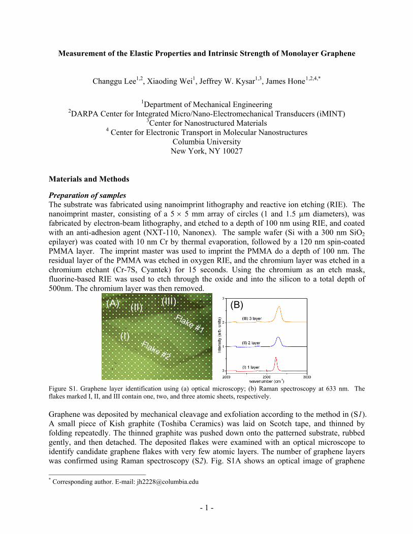
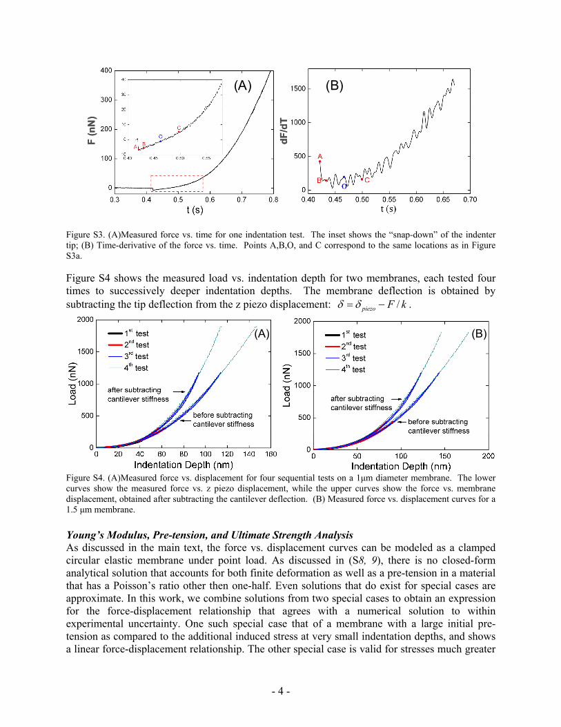
Figure S3. (A)Measured force vs. time for one indentation test. The inset shows the “snap-down” of the indenter tip; (B) Time-derivative of the force vs. time. Points A,B,O, and C correspond to the same locations as in Figure S3a. Figure S4 shows the measured load vs. indentation depth for two membranes, each tested four times to successively deeper indentation depths. The membrane deflection is obtained by subtracting the tip deflection from the z piezo displacement: /piezo F kδ δ= − .

Figure S4. (A)Measured force vs. displacement for four sequential tests on a 1μm diameter membrane. The lower curves show the measured force vs. z piezo displacement, while the upper curves show the force vs. membrane displacement, obtained after subtracting the cantilever deflection. (B) Measured force vs. displacement curves for a 1.5 μm membrane.

(A) (B)

Young’s Modulus, Pre-tension, and Ultimate Strength Analysis As discussed in the main text, the force vs. displacement curves can be modeled as a clamped circular elastic membrane under point load. As discussed in (S8, 9), there is no closed-form analytical solution that accounts for both finite deformation as well as a pre-tension in a material that has a Poisson’s ratio other then one-half. Even solutions that do exist for special cases are approximate. In this work, we combine solutions from two special cases to obtain an expression for the force-displacement relationship that agrees with a numerical solution to within experimental uncertainty. One such special case that of a membrane with a large initial pre-tension as compared to the additional induced stress at very small indentation depths, and shows a linear force-displacement relationship. The other special case is valid for stresses much greater

- 4 -

than the initial pre-tension, in which case the force varies as the cube of displacement. The sum of these two special cases is employed to analyze the data. For a clamped freestanding elastic thin membrane under point load, when bending stiffness is negligible and load is small, the relationship of force and deflection due to the pre-tension in the membrane derived by Wan et al. (S10) can be approximately expressed as: 2

0( )DF πσ= δ (S2)

where is applied force, F 20

Dσ is the membrane pre-tension, and δ is the deflection at the center point. When 1/ >>hδ , the relationship of deflection and force has been given by Komaragiri et al.(S9)

13

2

1D

Fa q E aδ ⎛= ⎜

⎝ ⎠⎞⎟ (S3)

where is the radius of the membrane, a 2DE is the two-dimensional Young’s Modulus, and 21/ .049 0.15 0.16 )q (1 ν ν= − − , with ν Poisson’s ratio (taken here as 0.165, the value for bulk

graphite). Summing the contribution of the pre-tension term and the large-displacement term, we can write

3

2 2 30 ( ) ( )D DF a E q a

a aδ δσ π ⎛ ⎞ ⎛ ⎞= +⎜ ⎟ ⎜ ⎟⎝ ⎠ ⎝ ⎠

. (S4)

The Young’s modulus, 2DE , and pre-tension, 20

Dσ , can be characterized by least-squares fitting the experimental curves using Eq. S4. This relationship, while approximate, is shown in Fig. S5 to agree with the numerical solution to within the uncertainty of the experiments. Since the point-load assumption yields a stress singularity at the center of the membrane, it is necessary to consider the indenter geometry in order to quantify the maximum stress under the indenter tip. Bhatia et al. (S11) derived the maximum stress for the thin clamped, linear elastic, circular membrane under a spherical indenter as a function of applied load

12 2

2

4

DD

mFE

Rσ

π⎛

= ⎜⎝ ⎠

⎞⎟ (S5)

where 2Dmσ is the maximum stress and R is the indenter tip radius. Eq. S5 suggests that the

breaking force is mainly a function of indenter tip radius, and is not affected by membrane diameter when , and this is consistent with our observation. As shown in Fig. 4a of the main paper, the breaking force with the 16.5 nm radius tip was about 1.8 μN for both membrane sizes (1 µm and 1.5 µm diameter), while the breaking force for the 27.5 nm radius tip was about 2.9 μN.

1/ <<aR

- 5 -

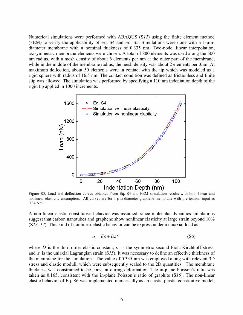
Numerical simulations were performed with ABAQUS (S12) using the finite element method (FEM) to verify the applicability of Eq. S4 and Eq. S5. Simulations were done with a 1-µm-diameter membrane with a nominal thickness of 0.335 nm. Two-node, linear interpolation, axisymmetric membrane elements were chosen. A total of 800 elements was used along the 500 nm radius, with a mesh density of about 6 elements per nm at the outer part of the membrane, while in the middle of the membrane radius, the mesh density was about 2 elements per 3nm. At maximum deflection, about 50 elements were in contact with the tip which was modeled as a rigid sphere with radius of 16.5 nm. The contact condition was defined as frictionless and finite slip was allowed. The simulation was performed by specifying a 110 nm indentation depth of the rigid tip applied in 1000 increments.

Figure S5. Load and deflection curves obtained from Eq. S4 and FEM simulation results with both linear and nonlinear elasticity assumption. All curves are for 1 μm diameter graphene membrane with pre-tension input as 0.34 Nm-1. A non-linear elastic constitutive behavior was assumed, since molecular dynamics simulations suggest that carbon nanotubes and graphene show nonlinear elasticity at large strain beyond 10% (S13, 14). This kind of nonlinear elastic behavior can be express under a uniaxial load as 2E Dσ ε ε= + (S6) where is the third-order elastic constant, D σ is the symmetric second Piola-Kirchhoff stress, and ε is the uniaxial Lagrangian strain (S15). It was necessary to define an effective thickness of the membrane for the simulation. The value of 0.335 nm was employed along with relevant 3D stress and elastic moduli, which were subsequently scaled to the 2D quantities. The membrane thickness was constrained to be constant during deformation. The in-plane Poisson’s ratio was taken as 0.165, consistent with the in-plane Poisson’s ratio of graphite (S16). The non-linear elastic behavior of Eq. S6 was implemented numerically as an elastic-plastic constitutive model,

- 6 -

since an elastic-plastic behavior is equivalent to a nonlinear elastic model as long as no unloading occurs.

Figure S6. Non-linear elastic properties of graphene (red dashed line) deduced from analysis of experiments. The diamond point denotes the maximum stress where slope is zero. The stress-strain curve from ab initio calculations by Liu et al. (S14) is the solid blue line.

It was assumed (based upon preliminary simulations) that the non-linear term in Eq. S6 would affect the stress primarily in the most highly strained portions of the membrane under or near the indenter. As a consequence, the predicted force-displacement curve was expected to be insensitive to , which implies that the use of the linear-elastic constitutive relationship in Eq. S4 is not inconsistent with the non-linear elastic constitutive relationship of Eq. S6. To validate this assumption, after determination of of E and (based upon the discussion below), the force-displacement response was simulated assuming a linear as well as a non-linear elastic relationship. As seen in Fig. S4, the difference between the force-displacement responses was smaller than the experimental uncertainties. Further the results indicated that only about 1% of the graphene membrane achieved a strain higher than about 5%, the threshold above which the non-linear term is important.

D

D

Therefore, the experimental force-displacement data sets were fit to Eq. S4 in order to determine the pre-tension, 2

0Dσ , and the elastic modulus, 2DE . A typical result is shown in Fig. 2a of the

main paper. The average value of Nm-1 (with standard deviation 40 Nm-1) was obtained based upon 67 force-displacement curves from 23 suspended graphene membranes (with diameters 1 μm and 1.5 μm) from two separate graphene flakes.

2 342DE =

The value of for most materials is negative, which reflects a softening of the elastic stiffness at large tensile strains, and graphene is no exception. 0

DGiven <D , the non-linear elastic

response predicts a maximum stress that can be supported by the material prior to failure, here

- 7 -

denoted as the intrinsic stress with value DE 42−= at thintσ e strain DE 2int −=ε . Beyond intε the slope of the stress-strain relationship is negative. FEM simulations of the deformed graphene membranes fail to find an equilibrium solution once the strains under the indenter tip have exceeded intε . The force on the indenter at the point of instability can then be interpreted as the breaking force of the membrane. Therefore, the value of D can be determined from the experimental data by matching the predicted breaking force with the mean value of the experimentally determined breaking force. Doing so yields a value of to 2 690DD = − Nm-1. This value is consistent with the breaking force for both indenter radii employed in the experiments.

Figure S7. Maximum stress vs. load curves obtained from Eq. S5 and FEM simulation results with both linear and nonlinear elasticity assumption with a 1 μm diameter graphene membrane and a 16.5 nm indenter radius. The resulting experimentally obtained stress-strain response based upon the non-linear constitutive form of Eq. S5 is shown in Figure S6. The resulting intrinsic stress is

at a strain of2 42Dintσ −= 1Nm int 0.25ε = .

- 8 -

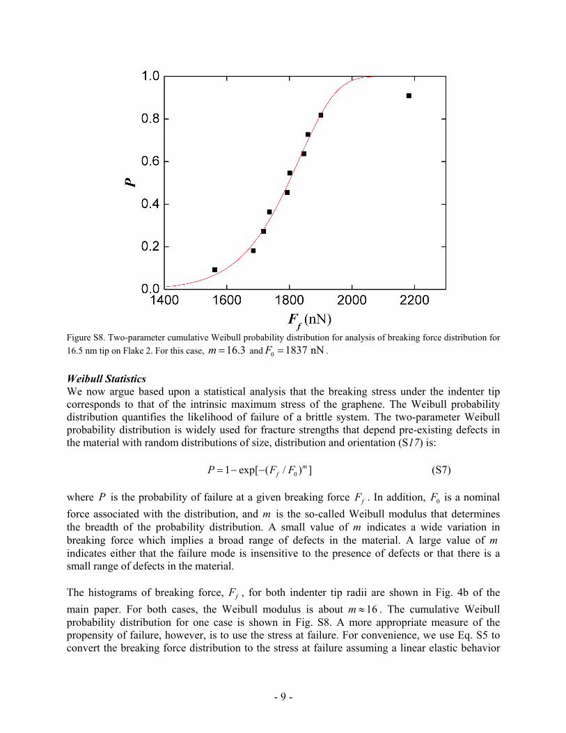
Figure S8. Two-parameter cumulative Weibull probability distribution for analysis of breaking force distribution for 16.5 nm tip on Flake 2. For this case, and16.3m = 0 1837 nNF = .

Weibull Statistics We now argue based upon a statistical analysis that the breaking stress under the indenter tip corresponds to that of the intrinsic maximum stress of the graphene. The Weibull probability distribution quantifies the likelihood of failure of a brittle system. The two-parameter Weibull probability distribution is widely used for fracture strengths that depend pre-existing defects in the material with random distributions of size, distribution and orientation (S17) is: (S7) 01 exp[ ( / ) ]m

fP F= − − F where is the probability of failure at a given breaking force . In addition, is a nominal force associated with the distribution, and m is the so-called Weibull modulus that determines the breadth of the probability distribution. A small value of m indicates a wide variation in breaking force which implies a broad range of defects in the material. A large value of m indicates either that the failure mode is insensitive to the presence of defects or that there is a small range of defects in the material.

P fF 0F

The histograms of breaking force, f , for both indenter tip radii are shown in Fig. 4b of the main paper. For both cases, the Weibull modulus is about 16

F≈m . The cumulative Weibull

probability distribution for one case is shown in Fig. S8. A more appropriate measure of the propensity of failure, however, is to use the stress at failure. For convenience, we use Eq. S5 to convert the breaking force distribution to the stress at failure assuming a linear elastic behavior

- 9 -

(which will be similar in trend to the non-linear elastic case as seen in Fig. S6). Since under those conditions, the maximum stress scales as the square root of fF , the Weibull modulus for the maximum stress di ion will be 30stribut ≈m , which implies a very narrow probability distribution. Experimental analysis for the distribution of breaking stresses of single and multi-walled carbon nanotubes (S18-20) has a very small Weibull m t ranges from

4odulus tha

~~75.1 << m and computer simulations of defects in graphene sheets suggest a value of 3≈m . In both of these cases, the small value of Weibull modulus indicates a very strong sensitivity of the breaking stress of the material as a function of the presence of initial defects. On the other hand, the high value of Weibull distribution, 30≈m , in the present experiments is indicative that the graphene membranes are entirely free of defects, at in the region of highest stress under the

nanome ich is the size scale of the ressed region under the AF

isp ent,

indenter tip.

ery highly st

Detailed measurements (S3) by Scanning Tunneling Microscopy (STM) of graphene sheets that were obtained from precisely the same Kish graphite source as in our work indicate that graphene sheets deposited in silicon substrates using the same methods as in our study have zero defects in them over an area of hundreds of squ

M tip.

ens shows that the d

are ters, wh

lacem

v Uncertainty Analysis Displacement sensing of the AFM was calibrated to estimate its accuracy using National Institute of Standards and Technology (NIST) traceable standard calibration gratings (S21), from Mikromasch (TGZ01: 18±1nm, TGZ02: 102±1.5nm, TGZ02: 498±6nm). Each grating was scanned at 9 different spots using contact scan mode, and the step heights were averaged. Calibration on those standard specim δ , measurement accu

depth is within 3.2%.

ty of the force measurem

racyup to 100 nm

he uncertain

ent, F k δ= ⋅T , is given as

2 2Δ Δ Δ⎛ ⎞

⎜ ⎟⎝ ⎠

(S8)

ius to be re ly small, the uncertainty easurement is approxim

F kF k

δδ

⎛ ⎞= +⎜ ⎟⎝ ⎠

dately

which gives accuracy of force measurement is about ±9.5% considering the error from spring constant, k , calibration, which is about 9%. From Eq. S4, assuming the uncertainty of the measurement of the tip radius and membrane ra lative of theelastic modulus m

2 2

E F3E F δδ

Δ Δ Δ⎛ ⎞⎜ ⎟⎝ ⎠

(S9) ⎛ ⎞= +⎜ ⎟⎝ ⎠

which yields 14%, so that the elastic modulus is 340 50± Nm-1. The pre-tension uncertainty should be of the same order as that of the Young’s modulus. From the nonlinear elasticity simulation results of maximum stress under the indenter tip shown in Fig. S6, we assume the empirical relationship for purposes of uncertainty evaluation to be

- 10 -

1/ 222 1/ 2

4

DD n

f fE F B F

Rπ⎛ ⎞

= + ⋅⎜ ⎟⎝ ⎠

. (S10)

intσ

he exponent is about as obtained by least-squares curve fitting of data points of 0.1n ≈ 2Dmσ T

fF in Fig. S6. Thus the uncertainty of 2Dintσand can be expressed as

222 2

2 2D D

- 11 -

2D Dint int

int fDf

E FE Fσ σσ

⎛ ⎞⎛ ⎞∂ ∂Δ = Δ + Δ⎜ ⎟⎜ ⎟ ⎜ ⎟∂ ∂⎝ ⎠ ⎝ ⎠

given above, Eq. S11 gives

. (S11)

From the uncertainty of Young’s modulus and force measurement accuracy of 2D

int as 10%. Therefore the intrinsic strength, 2Dσ intσ , is 42 ± 4 GPa.

inally, since , we can estimate an uncertain F ty of

DE 4/2int −=σ

2 22 2 2D D Dσσ

⎛ Δ

⎝ ⎠ ⎝ ⎠(S12)

ue of the third-order elastic modulus,

2 2 22 intD D D

D ED E

⎛ ⎞ ⎞Δ Δ= +⎜ ⎟ ⎜ ⎟ .

2DDThen the val , is -690 ± 120 Nm-1.

0, 3967 (1999).

Euen, R. C. Davis, Nano Lett. 6, 953 (2006). ech. Phys. Sol. 52, 2005 (2004).

. , 150 (2003).

64).

ridge, 1993). 18. A. H. Barber, I. Kaplan-Ashiri, S. R. Cohen, R. Tenne, H. D. Wagner, Composites Sci. Technol. 65, 2380 (2005). 19. N. M. Pugno, J. Phys.-Cond. Matt. 18, S1971 (2006). 20. N. M. Pugno, R. S. Ruoff, J. Appl. Phys. 99, (2006).

S21. NIST Reports 821/261141-99 and 821/265166-01.

References S1. K. S. Novoselov et al., Proc. Nat. Acad. Sci. USA 102, 10451 (2005). S2. A. C. Ferrari et al., Phys. Rev. Lett. 97, 187401 (2006). S3. E. Stolyarova et al., Proc. Nat. Acad. Sci. USA 104, 9209 (2007). S4. M. Tortonese, M. Kirk, SPIE 3009, (1997). S5. J. E. Sader, J. W. M. Chon, P. Mulvaney, Rev. Sci. Instrum. 7S6. B. Ohler. Veeco Application Note 94, http://www.veeco.com/library S7. J. D. Whittaker, E. D. Minot, D. M. Tanenbaum, P. L. McS8. M. R. Begley, T. J. Mackin, J. MS9. U. Komaragiri, M. R. Begley, J. App. Mech. 72, 203 (2005)S10. K. T. Wan, S. Guo, D. A. Dillard, Thin Solid Films 425S11. N. M. Bhatia, N. W., Int. J. Nonlin. Mech. 3, 307 (1968). S12. ABAQUS Inc., Pawtucket, RI S13. T. Xiao, X. J. Xu, K. Liao, J. Appl. Phys. 95, 8145 (2004). S14. F. Liu, P. M. Ming, J. Li, Phys. Rev. B 76, (2007). S15. R. N. Thurston, K. Brugger, Phys. Rev. 133, A1604 (19S16. O. L. Blakslee, J. Appl. Phys. 41, 3373 (1970). S17. B. Lawn, Fracture of Brittle Solids, 2nd Ed., (CambSSS