Supporting Information to ‘Spatial Distribution and ...xraysweb.lbl.gov/uxas/Publicatons/Papers/pdfs/Peggy2013_si.pdf · Supporting Information to ‘Spatial Distribution and Speciation

Supporting Information to

‘Spatial Distribution and Speciation of Arsenic in Peat Studied with

Microfocused X-ray Fluorescence Spectrometry and X-ray Absorption

Spectroscopy’

Peggy Langner,† Christian Mikutta,*,† Elke Suess,† Matthew A. Marcus,‡ and Ruben Kretzschmar†

†Institute of Biogeochemistry and Pollutant Dynamics, Department of Environmental Systems Science, ETH Zurich, 8092 Zurich, Switzerland

‡Advanced Light Source, Lawrence Berkeley National Laboratory, 1 Cyclotron Road, Berkeley, California 94720, United States

(9 Figures, 7 Tables)

Content:

1. Synchrotron measurements and data analyses ..................................................................... S2

2. Concentrations of major elements in peat cores B3II, B5II, and B1II ................................. S4

3. Bulk As, Fe, and S speciation results ................................................................................... S5

4. Synchrotron XRD analysis .................................................................................................. S7

5. Light microscopy analysis ................................................................................................... S8

6. Elemental correlation plots ................................................................................................ S10

7. Tricolor elemental maps .................................................................................................... S13

8. Thermodynamic data ......................................................................................................... S14

9. Eh-pH diagrams .................................................................................................................. S14

10. Arsenic concentrations in plants ........................................................................................ S16

11. References .......................................................................................................................... S18

Note: For the sake of clarity, the sample notation is confined to core label and mean sampling depth in centimeters: B1II-212, B1II-237, B3II-31, and B5II-12.

*Corresponding author’s e-mail: [email protected] Phone: +41-44-6336024; Fax: +41-44-6331118

Supporting Information to Langner et al.

S2

1. Synchrotron measurements and data analyses

Bulk X-ray absorption spectroscopy – As and Fe Arsenic K-edge (11867 eV) and Fe K-edge (7112 eV) X-ray absorption near edge structure (XANES) and extended X-ray absorption fine structure (EXAFS) spectra were collected over an energy range of 11667-12520 eV (As) and 6880-7794 eV (Fe). Higher harmonics in the beam were rejected by detun-ing the Si(220) double-crystal monochromators to 70% of their maximal intensity. The nominal ener-gy resolution ∆E/E was about ~10-4. The monochromators were calibrated relative to the L3-edge en-ergy of elemental Au (11919 eV) or the K-edge energy of elemental Fe (7112 eV). All samples were measured in fluorescence mode using solid-state Ge detectors with samples placed in a He cryostat (~10 K) at 45° relative to the incident beam. Four to eight scans per sample were collected and aver-aged. X-ray absorption spectroscopy (XAS) data analyses were performed using Athena.1-2 For spec-tra normalization, the Autobk algorithm was applied by fitting a linear function in the pre-edge region (E0-E = 30-140 eV for As and 30-130 eV for Fe) and a quadratic polynomial in the post edge region (E-E0 = 150-600 eV for As and 50-650 eV for Fe). E0 values were determined from the maximum of the first derivative of the measured XAS spectra. Linear combination fitting (LCF) of k3-weighted bulk As and Fe K-edge EXAFS spectra was performed over a k-range of 3-12 Å-1 utilizing a large set of As and Fe reference spectra.3

Bulk X-ray absorption spectroscopy – S Sulfur K-edge (2472 eV) XANES spectra were collected using a Si(111) double-crystal monochroma-tor (∆E/E ~10-4) and a Ni-coated harmonic rejection mirror. The sample stage was placed in a He at-mosphere in which the O2 content (typically <0.1%) was continuously monitored. Data collection was performed in fluorescence mode using a Lytle detector and with samples placed at 45° relative to the incident beam. All samples were measured at ~25 K using a liquid He cryostream. The monochroma-tor was calibrated relative to the white-line energy of a Na2S2O3 standard (2472.02 eV), which was repeatedly measured in between sample runs. Up to five scans were recorded in the energy range 2400-2650 eV for each peat sample. For spectra normalization in Athena, the Autobk algorithm was applied by fitting a linear function in the pre-edge region (E0-E = 15-70 eV) and a quadratic polyno-mial in the post edge region (E-E0 = 15-20 eV). E0 values were determined from the maximum of the first derivative of the measured XAS spectra. To identify oxidation states of S and quantify S species in the peat samples, data processing of the normalized S K-edge XANES spectra was carried out using WinXAS 3.24 following the fitting approach recommended by Manceau and Nagy.5 Deconvolution of the peat spectra into pseudo-components was performed in the energy range 2465-2490 eV using a series of Gaussians for the S s → p transition peaks and two arctangent functions. The positions of the Gaussians were chosen based on the white-line energy positions of S reference compounds.5-7 The first and second arctangent functions represent the edge step of reduced (2475.6 eV) and oxidized S species (2482.3 eV), respectively.5,8 The positions and widths of all Gaussians and arctangent func-tions were fixed, whereas the peak heights were allowed to vary in the fits. The areas of the Gaussians were calculated and subsequently corrected for the oxidation state-dependent change in the absorption cross-section based on the generic curve published in ref. 5. To calculate the relative contribution of every S species to the total S in the sample, the corrected peak area for each S species was normalized to the sum of all peak areas.


S3

Microfocused X-ray fluorescence spectrometry and X-ray absorption spectroscopy Elemental distribution maps of As, Fe, S, and other elements were collected with beam spot sizes be-tween 6 × 6 and 15 × 6 µm2 (H × V) and step sizes between 6 and 50 µm, depending on the size of the map. The thin sections were placed in a 45° angle to the incident beam, and the fluorescence signal was recorded at a 90° angle using a solid-state Ge detector. Each defined region was mapped at three incident photon energies: (1) 2802 eV (S, Si), (2) 7000 eV (Mn), and (3) 13001 eV (Fe, As). In each map, several points of interest (POI) were selected for extended As K-edge µ-XANES analysis in the energy range 11751-12192 eV. The spectra were dead-time corrected and averaged using software tools developed at ALS beamline 10.3.2.9 Linear combination fit analyses of the µ-XANES spectra were performed in Athena. The reference spectrum of arsenian pyrite used in the data evaluation was taken from ref. 10. The fit results were validated by the reconstruction of experimental k2-weighted µ-EXAFS spectra (k = 2-7 Å-1) based on the fitted fractions of As reference compounds.

Synchrotron X-ray diffractometry Diffraction patterns were collected at room temperature up to 120°2θ with an incident photon energy of ~20 keV (λ = 0.6199 Å) utilizing a solid-state Si microstrip detector (MYTHEN II). The experi-mental setup was calibrated using a Si powder standard (NIST 640c). Experimental powder patterns were evaluated with Match! 1.10d (Crystal Impact, Germany).


S4

2. Concentrations of major elements in peat cores B3II, B5II, and B1II

Table S1. Concentrations of major elements in peat cores B3II, B5II, and B1II. Values are given in g kg-1 dry weight except for As (mg kg-1).

Core Depth (cm)a Al As Cb Ca Fe K Mg Mn N P S Si B3II 12 (12) 6.45 551.1 377.5 7.01 19.3 2.41 0.93 0.19 19.7 0.61 5.91 35.8

31 (6) 17.2 271.5 336.4 6.35 12.7 4.64 2.31 0.12 17.5 0.84 5.73 52.3

44 (6) 55.9 54.5 134.8 5.37 17.8 13.0 5.30 0.23 9.62 1.48 2.72 148.3

62 (12) 65.4 39.3 148.2 6.11 13.7 13.7 4.36 0.21 8.42 1.63 2.34 158.9

87 (12) 61.5 67.3 173.1 9.54 15.5 11.1 3.98 0.17 5.20 1.58 4.69 114.9

112 (12) 58.0 19.3 9.00 9.36 25.1 15.4 9.03 0.42 0.03 0.60 0.23 165.7

B5II 12 (12) 51.0 397.1 122.2 7.19 35.1 13.7 7.49 0.36 8.12 1.18 2.83 134.3

37 (12) 52.8 323.4 108.4 6.92 29.4 13.4 7.60 0.33 8.23 1.24 2.61 165.5

62 (12) 59.6 438.9 22.3 6.80 29.2 15.6 9.06 0.37 1.65 1.09 1.28 182.9

87 (12) 69.9 580.1 58.7 7.25 35.1 16.5 10.4 0.38 4.96 1.97 1.59 178.8

112 (12) 73.0 444.6 56.1 7.54 34.3 17.3 10.1 0.40 3.88 1.93 1.25 173.6

137 (12) 74.0 321.2 59.8 7.87 27.8 17.4 9.08 0.36 3.22 2.08 1.50 166.5

B1II 12 (12) 32.3 55.2 247.3 6.97 21.3 7.69 4.08 0.22 17.0 1.12 6.07 115.1

37 (12) 22.8 60.1 299.4 6.01 13.7 5.19 2.77 0.15 17.8 0.77 5.97 79.0

62 (12) 9.65 38.2 356.3 4.69 8.26 2.31 1.08 0.08 25.0 0.50 5.95 48.7

100 (25) 43.9 14.3 183.3 6.50 11.8 11.7 3.15 0.17 11.9 1.04 3.08 132.0

137 (12) 18.5 35.5 291.2 7.25 12.6 5.44 1.07 0.13 15.9 0.74 6.14 57.4

162 (12) 4.57 87.2 439.4 13.4 6.85 1.15 0.32 0.03 19.5 0.37 12.1 9.00

187 (12) 2.20 233.3 452.8 14.0 5.70 0.42 0.26 0.02 20.2 0.26 15.5 2.41

212 (12) 2.21 331.0 452.8 14.1 4.69 0.53 0.41 0.03 21.3 0.28 15.3 3.06

237 (12) 11.8 255.7 348.4 11.7 8.28 4.12 1.39 0.08 12.7 0.39 16.6 34.5

262 (12) 37.1 66.0 158.7 12.7 18.8 12.5 4.92 0.22 6.46 0.55 14.5 119.8 aThe sampling depths are given as mean values with the sampling ranges (+/- mean value) in parentheses. Freeze-dried, homogenized, and ground (<50 µm) peat samples were analyzed by energy-dispersive X-ray fluorescence spectrometry (Spectro X-Lab 2000). Total C and N contents were determined in triplicate (mean relative standard deviation: 9.0%) with an elemental analyzer (Leco CHNS-932). brepresents organic C only because carbonates are absent as tested with 10% HCl.


S5

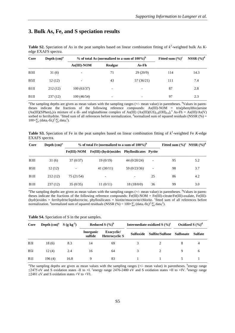
3. Bulk As, Fe, and S speciation results

Table S2. Speciation of As in the peat samples based on linear combination fitting of k3-weighted bulk As K-edge EXAFS spectra.

Core Depth (cm)a % of total As (normalized to a sum of 100%)b Fitted sum (%)c NSSR (%)d

As(III)-NOM Realgar As-Fh

B3II 31 (6) - 71 29 (20/9) 114 14.3

B5II 12 (12) - 43 57 (36/21) 111 7.4

B1II 212 (12) 100 (63/37) - - 87 2.8

B1II 237 (12) 100 (46/54) - - 97 2.3 aThe sampling depths are given as mean values with the sampling ranges (+/- mean value) in parentheses. bValues in paren-theses indicate the fractions of the following reference compounds: As(III)-NOM = tris(phenylthio)arsine (As(III)(SPhen)3)/a mixture of a di- and triglutathione complex of As(III) (As(III)(GS)2.6(OH)0.6),3 As-Fh = As(III)/As(V) sorbed to ferrihydrite. cfitted sum of all references before normalization. dnormalized sum of squared residuals (NSSR (%) = 100×∑i (datai-fiti)2/∑i datai

2).

Table S3. Speciation of Fe in the peat samples based on linear combination fitting of k3-weighted Fe K-edge EXAFS spectra.

Core Depth (cm)a % of total Fe (normalized to a sum of 100%)b Fitted sum (%)c NSSR (%)d

Fe(III)-NOM Fe(III)-(hydr)oxides Phyllosilicates Pyrite

B3II 31 (6) 37 (0/37) 19 (0/19) 44 (0/20/24) - 95 5.2

B5II 12 (12) - 41 (30/11) 59 (0/23/36) - 98 3.7

B1II 212 (12) 75 (21/54) - - 25 86 4.2

B1II 237 (12) 35 (0/35) 11 (0/11) 18 (18/0/0) 36 99 3.0 aThe sampling depths are given as mean values with the sampling ranges (+/- mean value) in parentheses. bValues in paren-theses indicate the fractions of the following reference compounds: Fe(III)-NOM = Fe(III)-citrate/Fe(III)-oxalate, Fe(III)-(hydr)oxides = ferrihydrite/lepidocrocite, phyllosilicates = biotite/muscovite/chlorite. cfitted sum of all references before normalization. dnormalized sum of squared residuals (NSSR (%) = 100×∑i (datai-fiti)2/∑i datai

2).

Table S4. Speciation of S in the peat samples.

Core Depth (cm)a S (g kg-1) Reduced S (%)b Intermediate oxidized S (%)c Oxidized S (%)d

Inorganic sulfide

Exocyclic/ Heterocyclic S

Sulfoxide Sulfite/Sulfone Sulfonate Sulfate

B3I 18 (6) 8.3 14 69 3 2 8 4

B5I 12 (4) 2.4 16 64 3 2 9 6

B1I 196 (4) 16.8 9 83 1 1 5 1 aThe sampling depths are given as mean values with the sampling ranges (+/- mean value) in parentheses. benergy range ≤2475 eV and S oxidation states -II to +I. cenergy range 2476-2480 eV and S oxidation states +II to +IV. denergy range ≥2481 eV and S oxidation states +V to +VI.


S6

Table S5. Peak parameters of deconvoluted S K-edge XANES spectra shown in Figure 2 and atomic fractions of S functionalities after correction for the oxi-dation-state dependent cross section of S.

Core Depth (cm)a White-line ener-gy (eV)

Assigned S func-tionality

Peak height Fwhm (eV)b Peak correction factorc

Uncorrected peak area

Corrected peak area

Corrected frac-tion (%)

NSSR (%)d

B3I 18 (6) 2470.50 inorganic sulfide 0.07 1.9 0.19 0.14 0.73 13.6 1.08

2472.90 exocyclic S 1.25 1.9 1.07 2.52 2.35 44.0

2474.30 heterocyclic S 1.04 1.9 1.59 2.11 1.33 24.8

2476.25 sulfoxide 0.21 1.9 2.31 0.43 0.19 3.5

2478.80 sulfite 0.21 2.0 3.24 0.44 0.14 2.6

2481.05 sulfonate 0.78 2.0 4.07 1.67 0.41 7.7

2482.80 sulfate 0.47 2.0 4.72 1.00 0.21 4.0


2472.90 exocyclic S 1.21 1.9 1.07 2.44 2.28 40.3

2474.30 heterocyclic S 1.03 1.9 1.59 2.08 1.31 23.2

2476.25 sulfoxide 0.22 1.9 2.31 0.45 0.19 3.4

2478.75 sulfite 0.21 2.0 3.23 0.44 0.14 2.4

2481.05 sulfonate 0.96 2.0 4.07 2.05 0.50 8.9

2482.80 sulfate 0.75 2.0 4.72 1.60 0.34 6.0


2473.25 exocyclic S 1.37 1.9 1.20 2.77 2.31 58.0

2474.60 heterocyclic S 0.83 1.9 1.70 1.67 0.98 24.7

2476.40 sulfoxide 0.03 1.9 2.36 0.05 0.02 0.6

2479.50 sulfone 0.09 2.0 3.50 0.18 0.05 1.3

2481.20 sulfonate 0.36 2.0 4.13 0.77 0.19 4.7

2482.90 sulfate 0.14 2.0 4.76 0.29 0.06 1.6 aThe sampling depths are given as mean values with the sampling ranges (+/-mean value) in parentheses. bfull width at half maximum. cbased on the ‘generic’ equation of Manceau and Nagy.5 dnormalized sum of squared residuals (NSSR (%) = 100×∑i (datai-fiti)2/∑i datai

2).


S7

4. Synchrotron XRD analysis

Figure S1. Synchrotron XRD patterns of the near-surface (B3II-31 and B5II-12) and deep peat layer samples (B1II-212 and B1II-237) analyzed by µ-XRF spectrometry and µ-XAS.


S8

5. Light microscopy analysis

Figure S2. (a, b) Photomicrographs of thin section B3II-31 in (a) plane-polarized light (PPL) and (b) cross-polarized light (CPL): Single plagioclase (A-B 1-2), quartz (A-B 2, A 3, C 1) and highly altered mica (D 4) par-ticles (~100-500 µm), as well as small ~1-3-mm sized rock fragments (e.g., gneiss: B 2, D 1-3) are embedded in the organic matrix. One example for each mineral and rock fragment is indicated in panel (b): Q = quartz, Pl = plagioclase, M = mica, and G = gneiss. (c, d) Photomicrographs of thin section B1II-237 in (c) PPL and (d) CPL: Organic matrix with small embedded quartz and mica particles of 10-50 µm size (not visible here). White boxes show the regions mapped by µ-XRF spectrometry (Figure 3).


S9

Figure S3. (a-c) Photomicrographs of thin section B3II-31 in (a, b) plane-polarized light (PPL) and (c) cross-polarized light (CPL). The white box in (a) indicates the location magnified in (b) and (c). In (c) reddish-brown secondary Fe-(hydr)oxides are present on mineral surfaces (A 1-2, A 4, C-D 1-3). (d-f) Photomicrographs of thin section B1II-212 in PPL (d, e) and CPL (f). The white box in (d) indicates region 1 mapped by µ-XRF spectrometry (Figure 4) and is magnified in (e) and (f). The CPL image also shows secondary Fe-(hydr)oxides with a reddish-brown color (A 3, B 4, D 2-3).


S10

6. Elemental correlation plots

Figure S4. Correlation plots of As and S fluorescence intensities and bicolor (RB) µ-XRF elemental maps illus-trating the distributions of As and S in (a-c) region 1 and (d-f) region 2 of thin section B3II-31, as well as (g-i) region 1 and (j-l) region 2 of thin section B1II-237 (Figure 3). The right-hand column displays µ-XRF maps generated from the orange points in the correlation plots. The color code in (c) is valid for all panels. Note that the scales of the x- and y-axis vary in the correlation plots.


S11

Figure S5. Correlation plots of relative As and Fe fluorescence intensities and bicolor (RG) µ-XRF elemental maps illustrating the distribution of As and Fe in (a-c) region 1 and (d-f) region 2 of thin section B3II-31, as well as (g-i) region 1 and (j-l) region 2 of thin section B1II-237 (Figure 3). The right-hand column displays µ-XRF maps generated from the orange points in the correlation plots. The color code in (c) is valid for all panels. Note that the scale of the y-axis varies in the correlation plots.


S12

Figure S6. Correlation plots of relative Mn and Fe fluorescence intensities and bicolor (RG) µ-XRF elemental maps illustrating the distribution of Mn and Fe in (a-c) region 1 and (d-f) region 2 of thin section B3II-31, as well as (g-i) region 1 and (j-l) region 2 of thin section B1II-237 (Figure 3). The right-hand column displays µ-XRF maps generated from the orange points in the correlation plots. The color code in (c) is valid for all panels. Note that the scales of the x- and y-axis vary in the correlation plots.


S13

7. Tricolor elemental maps

Figure S7. Tricolor (RGB) µ-XRF elemental maps of Mn, Fe, and Si in (a-c) thin section B3II-31 and (d-f) thin section B1II-237. (a, d) Overview maps indicating the locations of regions 1 and 2 mapped in each thin section. Fine maps of regions 1 are shown in (b, e) and those of regions 2 in (c, f). The color code in (f) is valid for all panels.


S14

8. Thermodynamic data

Table S6. Thermodynamic data used to calculate the change in Gibbs free energy of reaction (ΔG0).

Species/Reaction Mineral name ΔG0298 (kJ mol-1) log K Source

H2O -237.18 11

H+ 0 11

H2S -27.87 11

SO42- -744.5 12

H3AsO3 -639.73 13

Fe2+ -78.87 11

amorphous Fe(OH)3 ferrihydrite -712.95 14

FeS mackinawite -93.30 15

FeS troilite -97.91 14

FeS2 pyrite -160.23 16

Fe3S4 greigite -290.37 15

AsS realgar -33.18 17

FeAsS arsenopyrite -141.6 18

1/4CO2(g) + 11/12H+ + e- = 1/12lactate + 1/4H2O 0.68 19

9. Eh-pH diagrams

Pourbaix (Eh-pH) diagrams were calculated to illustrate the relative stabilities of realgar, orpiment, and arsenopyrite as a function of pH, redox potential, and varying abundances of Fe and S. The dia-grams were calculated with the Act2 program of the Geochemist’s Workbench package v.8.0 (Aque-ous Solutions LLC, USA). Arsenopyrite formation was implemented in the thermo_wateq4f database using Gibbs free energies of formation tabulated in Table S6 and a ∆G0 value of -141.6 kJ mol-1 for arsenopyrite:18

SO42- + Fe2+ + H3AsO3 + 11H+ + 11e- ↔ FeAsS + 7H2O ∆G0 = -338.76 kJ mol-1

Except for the AsS(OH)(HS)- and As3S4(HS)2- species already present in the data base, additional thi-

oarsenic species were disregarded in these calculations. Figure S8 shows Eh-pH diagrams calculated for a fixed log activity of -6 for As and different log activity ratios of Fe and S. The calculations indi-cate that under the ‘bulk’ redox conditions encountered in the peat (Eh = -11 to 364 mV) the solutions would be undersaturated with respect to all three As sulfide minerals. Arsenopyrite is predicted to be the most stable As sulfide at the slightly acidic pH of the peat (pH 5.7 ± 0.5). Based on the Eh-pH dia-grams, an authigenic arsenopyrite formation would be favored in microenvironments with redox po-tentials of approximately less than -100 mV. It must be stressed that if a ∆G0 value of -50.0 kJ mol-1 is used for arsenopyrite,20 this phase is predicted to be unstable under any conditions used to calculate the speciation diagrams. Thus, the new ∆G0 value of -141.6 kJ mol-1 for arsenopyrite18 is in better agreement with our field observations. A similar conclusion was reached by Craw et al.21 based on


S15

field observations focusing on natural and mined arsenopyrite occurrences in Otago Schist, New Zea-land.

In addition, our calculations show that realgar formation is generally more favorable under strongly reducing conditions preventing the formation of arsenopyrite (low Fe) and dissolved thioarsenic spe-cies (low Fe and S) (Figure S9).

Figure S8. Pourbaix diagrams (25°C, 1 bar) calculated for a fixed log activity of -6 for As and different log ac-tivity ratios of Fe and S in the As-Fe-O-H-S system.

∑As =-6, ∑Fe = -6, ∑S = -6

∑As =-6, ∑Fe = -6, ∑S = -4

∑As =-6, ∑Fe = -5, ∑S = -4

∑As =-6, ∑Fe = -4, ∑S = -4


S16

Figure S9. Pourbaix diagrams (25°C, 1 bar) calculated for different log activities of As (-6, -5) and S (-6 to -4) in the As-O-H-S system.

10. Arsenic concentrations in plants

Major plants species of the Gola di Lago peatland were collected in September 2009 within a radius of 3 m around the sampling points B1, B3, and B5. Approximately 10 plants of each species were harvested, immediately shock frozen in liquid N2, transported on dry-ice in the laboratory, and stored at -22°C before further processing. An overview of all collected plant species and their abundance according to the Braun-Blanquet scale22 is given in Langner et al.3

The frozen samples were washed several times with tap water, rinsed with deionized water, and freeze-dried for 72 h. The individual plants of each species were then combined into one sample and separated into root, stem/leaf, and blossom, which were subsequently homogenized in a ZrO2 ball mill (Retsch, MM 200) for 4 min at 24 s-1. Aliquots of the ground plant material (0.2 g) were then added to 1.5 mL ultrapure water (18.2 MΩ cm, Millipore), 2.5 mL HNO3 (67% w/w), and 1.5 mL H2O2 (30% w/w) and digested in triplicate using a MLS microwave (turboWave®, MLS GmbH). The sam-ples were pre-reacted for one hour and digested for 25 min at a maximal pressure and temperature of

∑As =-6, ∑S = -6

∑As =-6, ∑S = -5

∑As =-6, ∑S = -4

∑As =-5, ∑S = -4


S17

120 bar and 250°C, respectively. The efficiency of the digestion procedure was validated with various reference materials (olive leaves (BCR®-062), apple leaves (SRM NIST 1515) as well as bush branches and leaves (NIM-GBW07603, NCS DC73349)). The digests were diluted to 10 mL with ultrapure water and analyzed for As by inductively coupled plasma – mass spectrometry (Agilent, 7500 Series) in addition to other elements needed for quality control. The average and blank corrected As concentrations, calculated on a dry weight basis, are reported in Table S7.

Table S7. Arsenic concentrations in plants collected at sampling sites B1, B3, and B5.

Common name Species Family Part of the plant As (mg kg-1)

B3

Purple moorgrass Molinia caerulea Poaceae blossom 2.82

leaf/stem 0.41

root 1.88

Smooth black sedge Carex nigra Cyperaceae leaf/stem 10.1

root 78.5

Sphagnum Sphagnum sp. Sphagnaceae leaf/stem 1.67

Jointleaf rush Juncus articulatus Juncaceae blossom 11.9

leaf/stem 5.93

root not determined

B5


leaf/stem 0.14

root 26.7

Smooth black sedge Carex nigra Cyperaceae leaf/stem 2.12

root 0.17

Water whorlgrass Catabrosa aquatica Poaceae leaf/stem 0.19

root 0.86

Jointleaf rush Juncus articulatus Juncaceae blossom 0.37

leaf/stem 0.13

root 1.62

B1


leaf/stem 0.19

root 7.34

Tufted bulrush Trichophorum cespitosum Cyperaceae leaf 0.32

root 7.85

Mean 7.05

Standard deviation 16.7


S18

11. References

(1) Ravel, B. and Newville, M. Athena, Artemis, Hephaestus: data analysis for X-ray absorption spectroscopy using Ifeffit. J. Synchrot. Radiat. 2005, 12, 537-541.

(2) Ravel, B. and Newville, M. Athena and Artemis: interactive graphical data analysis using Ifeffit. Phys. Scr. 2005, T115, 1007-1010.

(3) Langner, P.; Mikutta, C. and Kretzschmar, R. Arsenic sequestration by organic sulphur in peat. Nat. Geosci. 2012, 5, 66-73.

(4) Ressler, T. WinXAS: a program for X-ray absorption spectroscopy data analysis under MS-Windows. J. Synchrot. Radiat. 1998, 5, 118-122.

(5) Manceau, A. and Nagy, K. L. Quantitative analysis of sulfur functional groups in natural organic matter by XANES spectroscopy. Geochim. Cosmochim. Acta 2012, 99, 206-223.

(6) Hoffmann, M.; Mikutta, C. and Kretzschmar, R. Bisulfide reaction with natural organic matter enhances arsenite sorption: insights from X-ray absorption spectroscopy. Environ. Sci. Technol. 2012, 46, 11788–11797.

(7) Vairavamurthy, A. Using X-ray absorption to probe sulfur oxidation states in complex molecules. Spectrochim. Acta, Part A 1998, 54, 2009-2017.

(8) Xia, K.; Weesner, F.; Bleam, W. F.; Bloom, P. R.; Skyllberg, U. L. and Helmke, P. A. XANES studies of oxidation states of sulfur in aquatic and soil humic substances. Soil Sci. Soc. Am. J. 1998, 62, 1240-1246.

(9) Marcus, M. A. and Fakra, S. C. µXAS & µEXAFS on beamline 10.3.2. http://xraysweb.lbl.gov/uxas/Index.htm.

(10) Bostick, B. C. and Fendorf, S. Arsenite sorption on troilite (FeS) and pyrite (FeS2). Geochim. Cosmochim. Acta 2003, 67, 909-921.

(11) Stumm, W. and Morgan, J. J. Aquatic chemistry. Chemical equilibra and rates in natural waters. 3rd ed.; John Wiley & Sons, Inc.: New York, 1996.

(12) Shock, E. L. and Helgeson, H. C. Calculation of the thermodynamic and transport properties of aqueous species at high pressures and temperatures: correlation algorithms for ionic species and equation of state predictions to 5 kb and 1000°C. Geochim. Cosmochim. Acta 1988, 52, 2009-2036.

(13) Vink, B. W. Stability relations of antimony and arsenic compounds in the light of revised and extended Eh-pH diagrams. Chem. Geol. 1996, 130, 21-30.

(14) Lindsay, W. L. Chemical equilibria in soils. John Wiley & Sons, Inc.: New York, 1979. (15) Berner, R. A. Thermodynamic stability of sedimentary iron sulfides. Am. J. Sci. 1967, 265,

773-785. (16) Robie, R. A.; Hemingway, B. S. and Fisher, J. R. Thermodynamic properties of minerals and

related substances at 298.15 K and 1 bar (105 Pascal) pressure and at higher temperatures. U.S. Geological Survey Bulletin 1452: Washington, 1978.

(17) Pokrovski, G.; Gout, R.; Schott, J.; Zotov, A. and Harrichoury, J. C. Thermodynamic properties and stoichiometry of As(III) hydroxide complexes at hydrothermal conditions. Geochim. Cosmochim. Acta 1996, 60, 737-749.

(18) Pokrovski, G. S.; Kara, S. and Roux, J. Stability and solubility of arsenopyrite, FeAsS, in crustal fluids. Geochim. Cosmochim. Acta 2002, 66, 2361-2378.

(19) Morel, F. M. M. and Hering, J. G. Principles and applications of aquatic chemistry. John Wiley & Sons, Inc.: New York, 1993.

(20) Gallegos, T. J.; Han, Y.-S. and Hayes, K. F. Model predictions of realgar precipitation by reaction of As(III) with synthetic mackinawite under anoxic conditions. Environ. Sci. Technol. 2008, 42, 9338-9343.

(21) Craw, D.; Falconer, D. and Youngson, J. H. Environmental arsenopyrite stability and dissolution: theory, experiment, and field observations. Chem. Geol. 2003, 199, 71-82.

http://xraysweb.lbl.gov/uxas/Index.htm


S19

(22) Braun-Blanquet, J. Plant sociology: the study of plant communities. McGraw-Hill: New York, 1932.

Documents

Supporting Information to ‘Spatial Distribution and ...xraysweb.lbl.gov/uxas/Publicatons/Papers/pdfs/Peggy2013_si.pdf · Supporting Information to ‘Spatial Distribution and Speciation