Embed Size (px)
Citation preview
Supporting Finite Element Analysis with a Relational Database Backend Part III: OpenDX – Where the Numbers Come Alive
Gerd Heber, Chris Pelkie, Andrew Dolgert Cornell Theory Center, [638, 622, 634] Rhodes Hall,
Cornell University, Ithaca, NY 14853, USA [heber, chrisp]@tc.cornell.edu, [email protected]
Jim Gray Microsoft Research, San Francisco, CA 94105, USA
David Thompson Visualization and Imagery Solutions, Inc.,
5515 Skyway Drive, Missoula, MT 59804, USA [email protected]
December 2005
Technical Report
MSR-TR-2005-151
Microsoft Research
Microsoft Corporation
One Microsoft Way
Redmond, WA 98052
- 2 -
Supporting Finite Element Analysis with a Relational Database Backend
Part III: OpenDX – Where the Numbers Come Alive Gerd Heber*, Chris Pelkie*, Andrew Dolgert*, Jim Gray†, and David Thompson‡
*Cornell Theory Center, [638, 622, 634] Rhodes Hall, Ithaca, NY 14853, USA
[email protected], [email protected], [email protected]
†Microsoft Research, 455 Market St., San Francisco, CA 94105, USA
‡Visualization and Imagery Solutions, Inc.
5515 Skyway Drive, Missoula, MT 59804, USA
Abstract: In this report, we show a unified visualization and data analysis approach to Finite Element Analysis (FEA). The example application is visualization of 3-D models of (metallic) polycrystals. Our solution combines a mature, general-purpose, rapid-prototyping visualization tool, OpenDX (formerly known as IBM Visualization Data Explorer) [1,2], with an enterprise-class relational database management system, Microsoft SQL Server [3]. Substantial progress can be made with established off-the-shelf technologies. This approach certainly has its limits and we point out some of the shortcomings which require more innovative products for visualization, data, and knowledge management. Overall, the approach is a substantial improvement in the FEA life cycle, and probably will work for other data-intensive sciences wanting to visualize and analyze massive simulation or measurement data sets.
Introduction
This is certainly not the first report on the intriguing combination of a database server and a visualization environment. Early reports date back to the late eighties and early nineties. Imagining the comparatively immature state of database systems, visualization tools, and middleware of that period, we admire the vision and courage of those early adopters. We can understand that after living on the bleeding edge of technology, some of those pioneers abandoned the idea of combining databases and visualization. The main message of this report is that things have evolved to a point that, for a large class of applications, the unification of off-the-shelf visualization tools and database systems can work very well to support both the actual FEA simulation workflow and data management and for the post-production data analysis tasks. The tools have certainly matured, but it is the scale and complexity of the data coming from the applications that renders ad hoc data management and data visualization increasingly impractical. More systematic and general approaches are needed.
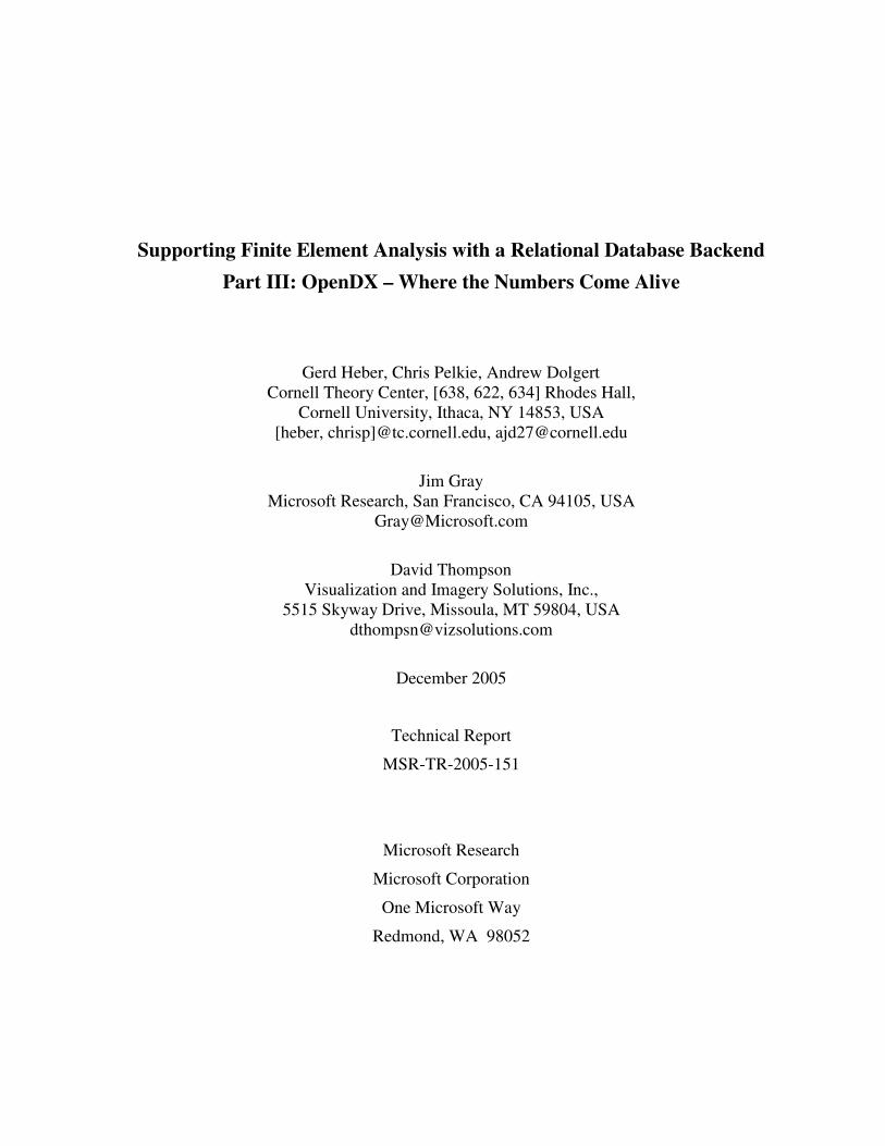
Much of the work presented in this report was done in support of the DARPA-SIPS (Structural Integrity and Prognosis System) effort, which aims to substantially improve life predictions for hardware like the Northrop Grumman EA-6B aircraft by using better material science and better multi-scale analysis. One ingredient in an aircraft’s remaining life assessment is the maximum flaw size (crack length) detected in a certain borehole of one of its outer wing panels. If this flaw size exceeds a critical value the aircraft is considered to have lost its structural integrity and is taken out of service. At the length scale in question, the material of the wing panel (Al 7075) shows a microstructure that material scientists commonly refer to as a polycrystal structure (see Appendix A). So, analyzing
Figure 1: The image on the left shows a Northrop Grumman EA-6B of the U.S. Navy. The right image is a close-up of a bolt hole surface.

Supporting Finite Element Analysis with a Relational Database Backend 3
polycrystal structures using finite element analysis is a key ingredient to estimating the useful remaining life of an aircraft.
In this article, we first explain the basic concepts of metallic polycrystals and how they are conceptualized in a finite element analysis. Next, we discuss how this conceptual model can be mapped to a relational data model, and we present a requirements analysis for polycrystal visualization. We provide a detailed description of our implementation using OpenDX, Microsoft SQL Server 2005, and Python. An example screen snapshot of the visualization system is shown in Figure 2. Before reading this report, we highly recommend watching a 6 minute video clip [18] which demonstrates the system in use. After that the reader may decide how much she wants to know about the innards.
Figure 2: A visualization interface for finite element analysis of polycrystals showing: the visualization data flow in the upper left panel, interactive visualization controls in the upper right and lower left, and a histogram and 3-D visualization of the data in the two foreground panes. The displays can be animated to show how the model behaves over time. Displays like this are constructed during all phases of finite element analysis. The system pulls data from the database, transforms it, and then renders it in intuitive ways allowing the investigator to explore the model’s structure and behavior.
Modeling Polycrystals
Polycrystals are inhomogeneous materials composed of crystal domains. Granite is a familiar polycrystalline material, but most metals and many other materials consist of crystalline grains, each grain being homogenous. (See Figure 1 and Appendix A for scans of a real microstructure.) The information underlying three-dimensional models of (metallic) polycrystals can be organized in a hierarchy of topological, geometric, discretization, physical, and engineering data.1 Figure 3 shows a small part of a polycrystal dictionary.
1 Particles and inclusions, which are an important ingredient in modeling realistic grain structures, are beyond the scope of this presentation. The reader can think of them as special grains inside of or in-between other grains.
Figure 3: Part of a polycrystal ontology (OWLViz [27]). Basic concepts include topological, geometric, and mesh entities. Dimension is a topological entity’s’ main attribute. It is related to other topological entities via the incidence or boundary relation. Topological entities can be embedded into 3-space and have geometric realizations that map vertices onto points and faces onto polygons. A mesh represents the decomposition of a volume into simple shapes (bricks, tetrahedra etc.). The fundamental relation (the glue) between mesh objects is the subset relation. Sets of mesh entities segment geometric entities; for example, curves are segmented into edges, and polygons can be segmented into triangles and/or quadrilaterals.
- 4 -
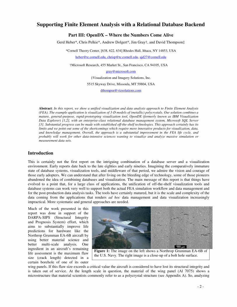
Vertices, strings (edges, loops), faces, and regions (grains) are the basic topological objects. Edges connect vertex pairs. Ordered (oriented) sets of topological vertices form loops, one or more of which bound planar faces. Each region is bounded by one or more topological faces. Assigning Cartesian coordinates to vertices embeds them into Euclidean space. This turns a polycrystalline topology into a geometric object—the grains become polyhedra, with planar polygonal bounding faces. Figures 4 and 5 show examples of polycrystalline geometries.
Faces and regions are tessellated (subdivided) in order to represent each crystal as a finite element mesh (see Figure 4). The tessellation of the faces is also referred to as the surface mesh. Surfaces include the external as well as the internal grain boundaries. The surface mesh typically consists of triangles and/or quadrilaterals. The tessellation of the grains is referred to as the volume mesh. It typically consists of tetrahedra or a mixture of elements including bricks, prisms, and pyramids. The surface and volume meshes are compatible, i.e., the footprint of the volume elements matches exactly the (initial) surface mesh.
The geometry and mesh generation for polycrystals is quite challenging. The goal is to generate realistic geometries with “good quality” surface and volume meshes and with as few elements as possible. Minimizing the number of elements keeps the size of the underlying system of nonlinear finite element equations under control while providing good model fidelity. The size and element quality of the surface mesh determines the resolution of boundary conditions as well as a characteristic length scale on the grain interfaces. The quality of the surface mesh directly impacts the difficulty of volume mesh generation, if an advancing front mesh generator2 is used for that purpose. Octree-based techniques appear inadequate, because a given surface mesh cannot be enforced and good quality surface/volume meshes tend to be significantly larger, leading to intractably large systems of equations. The density of the resulting mesh varies depending on the complexity of the geometry. The mesh typically does not change for an individual analysis unless, for example, a convergence study is performed.
2 Roughly speaking, an advancing front mesh generator creates a volume mesh by starting from the surface mesh and “growing”
elements from the front between tessellated and un-tessellated space. The procedure terminates when the front collapses and the volume is filled with elements.
Figure 4: A surface mesh for a grain geometry. A conforming tetrahedral mesh extends into the interior of the grains. Depending on its size and the complexity of the surface mesh, each grain is decomposed into hundreds or thousands of tetrahedra. The tessel-lations respect the grain topology: there is exactly one mesh vertex coincident with each grain vertex. Each topological loop is segmented by mesh edges. Each surface triangle or quadrilateral is “owned” by exactly one topological face and each volume element (tetrahedron, hexahedron, prism, or pyramid) is “owned” by (is inside) exactly one grain.
Figure 5: Three examples of polycrystal geometries. The grains are shrunk for visualization purposes. The corners of the grains correspond to topological vertices. Grains are bounded by planar faces, which in turn are bounded by oriented loops (the orientation determines the “inside” of the region to allow faces with holes). In the upper image, all topological faces are bounded by exactly one topological loop. (Multiple loops are required to represent faces with holes.) The upper geometry was created from a Voronoi tessellation [17] so all grains are convex domains. Physically more realistic grain geometries, such as the one shown in the middle image, generally have some concave faces and exhibit various anisotropies. The bottom image shows a polycrystal with very simple grains that captures grain anisotropy (elongation) after the rolling of the raw material.
Supporting Finite Element Analysis with a Relational Database Backend 5
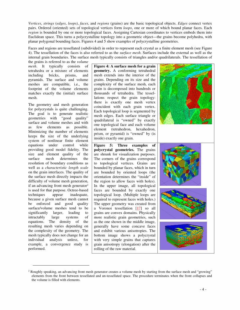
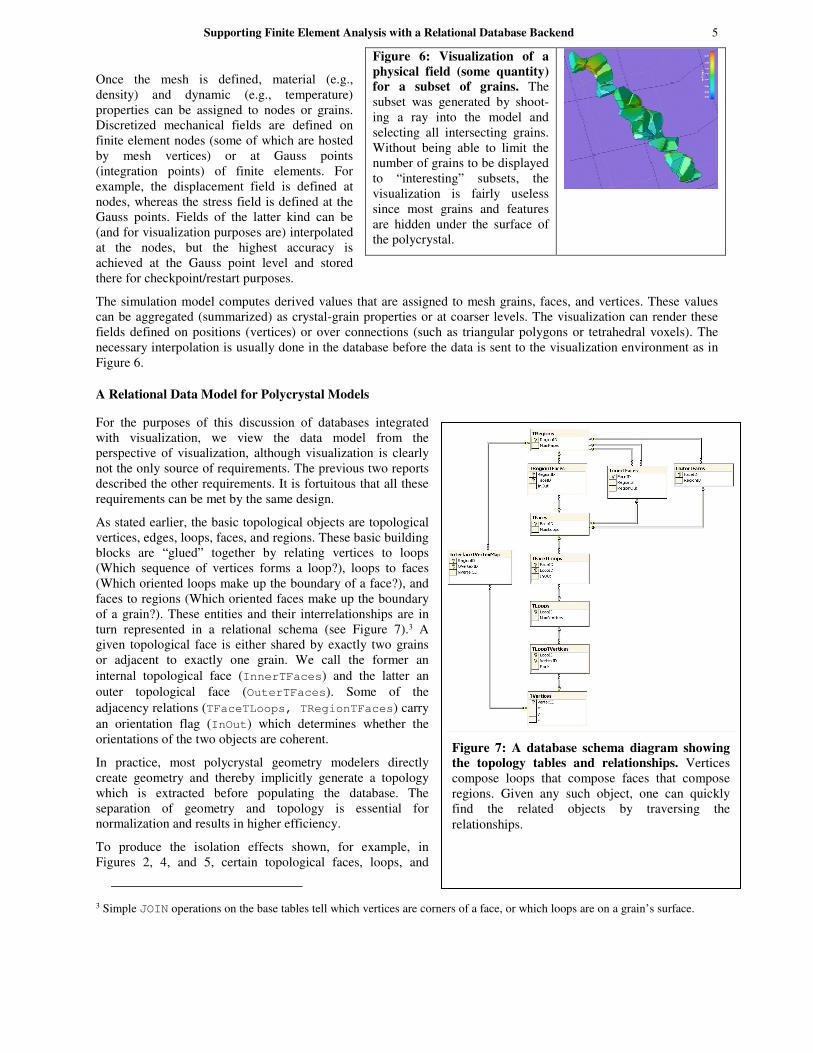
Figure 7: A database schema diagram showing the topology tables and relationships. Vertices compose loops that compose faces that compose regions. Given any such object, one can quickly find the related objects by traversing the relationships.
Once the mesh is defined, material (e.g., density) and dynamic (e.g., temperature) properties can be assigned to nodes or grains. Discretized mechanical fields are defined on finite element nodes (some of which are hosted by mesh vertices) or at Gauss points (integration points) of finite elements. For example, the displacement field is defined at nodes, whereas the stress field is defined at the Gauss points. Fields of the latter kind can be (and for visualization purposes are) interpolated at the nodes, but the highest accuracy is achieved at the Gauss point level and stored there for checkpoint/restart purposes.
The simulation model computes derived values that are assigned to mesh grains, faces, and vertices. These values can be aggregated (summarized) as crystal-grain properties or at coarser levels. The visualization can render these fields defined on positions (vertices) or over connections (such as triangular polygons or tetrahedral voxels). The necessary interpolation is usually done in the database before the data is sent to the visualization environment as in Figure 6.
A Relational Data Model for Polycrystal Models
For the purposes of this discussion of databases integrated with visualization, we view the data model from the perspective of visualization, although visualization is clearly not the only source of requirements. The previous two reports described the other requirements. It is fortuitous that all these requirements can be met by the same design.
As stated earlier, the basic topological objects are topological vertices, edges, loops, faces, and regions. These basic building blocks are “glued” together by relating vertices to loops (Which sequence of vertices forms a loop?), loops to faces (Which oriented loops make up the boundary of a face?), and faces to regions (Which oriented faces make up the boundary of a grain?). These entities and their interrelationships are in turn represented in a relational schema (see Figure 7).3 A given topological face is either shared by exactly two grains or adjacent to exactly one grain. We call the former an internal topological face (InnerTFaces) and the latter an outer topological face (OuterTFaces). Some of the adjacency relations (TFaceTLoops, TRegionTFaces) carry an orientation flag (InOut) which determines whether the orientations of the two objects are coherent.
In practice, most polycrystal geometry modelers directly create geometry and thereby implicitly generate a topology which is extracted before populating the database. The separation of geometry and topology is essential for normalization and results in higher efficiency.
To produce the isolation effects shown, for example, in Figures 2, 4, and 5, certain topological faces, loops, and
3 Simple JOIN operations on the base tables tell which vertices are corners of a face, or which loops are on a grain’s surface.
Figure 6: Visualization of a physical field (some quantity) for a subset of grains. The subset was generated by shoot-ing a ray into the model and selecting all intersecting grains. Without being able to limit the number of grains to be displayed to “interesting” subsets, the visualization is fairly useless since most grains and features are hidden under the surface of the polycrystal.

- 6 -
vertices need to be replicated.4 Even if visualization tools supported this for arbitrary polyhedra (they don’t!), there are good reasons to duplicate topological features in the model. When modeling the mechanical response of a polycrystal, the grains are assigned material properties following certain statistical distributions. The interfaces between the grains — the grain boundaries — are either assumed to be of infinite strength or they are assigned material properties which allow them, following a certain constitutive law, to soften or break (de-cohere). In other words, duplicate entities are needed to support the physical modeling of the two sides of grain boundary behavior. As a result, two polycrystal models are stored in the database, one with and one without duplicate entities. A client application can select whichever view is appropriate. The object replication is implemented within the database as a stored procedure that replicates topological vertices (the number of copies depends on the number of sharing grains) and that generates a multi-valued mapping (InterfaceTVertexMap in Figure 7) from the unduplicated to the replicated topology. The replica can then be easily obtained via JOIN with the InterfaceTVertexMap table.
A mesh generator is used to decompose the polycrystal geometry into simple shapes that respect the topological structure of the model. For each topological vertex there is exactly one coincident mesh vertex. Each topological loop is split into a chain of mesh edges. Each topological face is divided into triangles and/or quadrilaterals. Each grain is tessellated with tetrahedra, hexahedra, prisms, or pyramids. The fundamental relation is the element-vertex adjacency relation. Besides the basic objects (vertices, elements) and this relation, we have to store the mappings of mesh edges to topological loops and triangles to topological faces. (The fact that two vertices are on the same loop and may be even closer than any two other vertices on that same loop does not imply that there is a mesh edge between them.)
The topology replication carries through to the mesh level. The mapping defined at the topology level is “pushed down” to the finer mesh level. Mesh objects in the interior of grains are unaffected by this replication. However, vertices, edges, triangles, etc., on grain surfaces need to be duplicated accordingly. In addition, the vertices of elements adjacent to internal grain interfaces have to be remapped. At this point, special elements so-called interface elements which model the mechanical response of the grain interfaces, are introduced. The reader can think of them as triangular prisms (wedges) or bricks of zero thickness. They are generated by extrusion from the triangles and/or quadrilaterals that form the surface mesh on the internal faces.
The two meshes (with and without duplication) can be used to define finite elements. The resulting node sets are kept separate from the meshes, because the same mesh topology can be used to define different finite element meshes depending on, for example, the order of the shape functions5. A node set is defined by a choice of a mesh (replicated, unreplicated) and a shape function order (linear, quadratic, etc.). We typically store four node sets in a database.
Following our metadata discussion in Part I [3], mesh attributes like boundary conditions and material properties are stored in XML documents. Client-side scripts and user-defined functions consume these documents to instantiate attributes for the FEA.6 A complete set containing a finite element mesh and attributes defining a unique solution is called a case. The resulting fields and state variables from an FEA case are stored in tables tagged with their case ID. In practice, there are around 80 cases for each model. This is a fairly sizeable subset of all possible combinations of shape functions, boundary conditions, and material models and properties. (Certain combinations are impossible: For example, if a material model requires quadratic shape functions, it cannot be combined with linear shape functions.)
The final schema has about 65 tables, 25 views, and 80 user-defined functions (stored procedures, scalar- and table-valued functions.) Data sets from simulations result in additional tables for case-dependent state variables. The latter tables are by far the storage dominant part (99%). The former serve as metadata to interpret the latter. The relatively large number of tables is due the number of modeling dimensions (with or without interfaces, with or without particles, linear or quadratic elements, etc.).
4 Note that the term ‘replicate’ is used in the sense of ‘creating copies’ leaving the number of copies unspecified. For internal
faces, exactly two copies of that face are created. Generally the same is not true for either a face’s bounding loops or its vertices.
5 For higher order shape functions, certain associations between nodes and mesh entities must be stored. For example, quadratic elements have nodes associated with the midpoints of their edges.
6 The XML support in SQL Server 2005 allows doing most of the XML processing on the server (via XQuery) and the full documents are actually never transferred to the client.

Supporting Finite Element Analysis with a Relational Database Backend 7
Visualization Requirements
The following are some key requirements for an environment to visualize models of polycrystals:
1. The environment must be able to display all aspects and forms of (meta-) data associated with polycrystals, including topology/geometry, (FEM) discretization, and physics/mechanics.
2. It must scale to models with ~105 grains. At the same time, it must be able to adapt to different resource constraints and models of increasing size. For example, it must prevent users from requesting amounts of data which exceed their local resources.
3. The environment must be a rapid-prototyping environment. All excessive and needless programming must be avoided.
4. The environment must allow nearly real-time interaction with the models.
5. The underlying data sources and data access must be self-describing, aid self-configuring applications, and accommodate relational, image, and XML data.
6. The system can only use standard off-the-shelf hardware and software.
We want a tool that works for the entire FEA process from model definition, to topology/geometry generation, to discretization, to simulation, and then to numerical analysis, visualization, and post-processing.
To be physically relevant, models must have at least 10,000 grains. For models with more than 100 grains, it is difficult for an end-user to estimate the amount of data involved in a display request. Certain safeguards must be built into the system to maintain a highly responsive system, hence the second requirement.
It must be easy to extend or add new visual components. A good visualization is often the result of experimentation, of trial and error. Environments which do not support rapid prototyping hinder and discourage the willingness to experiment, and result in sub-optimal visualization. The real time interaction is essential to allow people to interact with and explore the data — it vastly improves productivity.
Requirement 5, self-describing data, echoes the first requirement and goes beyond the scope of visualization. Since the visualization environment shares almost all data with other applications and the underlying data sets are quite large, replication must be avoided and a special purpose data repository for visualization alone seems undesirable.
The requirement for commodity hardware and software is economic in nature: it keeps accessibility high and does not require us to reinvent the wheel.
OpenDX
OpenDX (or “DX”)7 is a visual programming environment whose main purpose is to produce visual representations of data. That is, to “write a program,” we select and place graphical boxes called modules — representing (in a loose sense) “functions” — on a workspace (the canvas), then we drag connecting wires between these boxes. The wires indicate data-flow paths from outputs of upstream modules to the inputs of downstream modules. No explicit wiring loop-backs (circular logic) are permitted; some situations that resemble loop-backs are explained later.
Each module is, of course, already precompiled for the host architecture. The DX Executive (“dxexec”) process runs separately from the DX User Interface (“dxui”) process and watches while you program, assembling the execution dependency graph. In fact, DX will prevent you from creating a loop-back or from making some other types of illegal connections. When a valid network program (a net in DX-speak) has been constructed, it may be immediately executed. No compilation is necessary and, generally speaking, execution is quite rapid. Naturally, extremely large data sets require more time to read in, and there are a few modules whose very nature makes them slow, but most nets exhibit quite acceptable performance.
7 OpenDX was originally developed and marketed for several years by IBM’s Watson Research group as IBM Visualization Data Explorer. It was open-sourced in 1998 and is now freely available [1]. The user interface requires X Windows, though there is a project to create a native Microsoft Windows version discussed later in this report. In the interim, on our Windows machines, we use Hummingbird Exceed’s X-server product.
- 8 -
Successive executions run even faster, since, by default, DX caches all intermediate results in local memory. Pointers to cache objects are passed from module to module; only those data components that change are duplicated in memory before being modified.8 And only those modules whose inputs change require re-execution.
The chief input channel to OpenDX from the outside world is the Import module, and it is most commonly used to directly open a static file from disk. However, Import offers a powerful alternative input scheme which we employ in the polycrystal viewer. In place of an explicit pathname/filename, one can substitute a string of the form:
!executable (e.g., script name, compiled program, etc.) arg1 arg2 …
The bang (!) indicates that the executable directive is to be handed to the operating system where it runs using the supplied arguments. The implicit output “pipe” connects to OpenDX’s standard input. When the executable returns, it must write a stream in the form of a valid OpenDX object. OpenDX blocks until the stream is complete, whereupon it proceeds in normal fashion to process and render the data object as an image. From our PreView and PView nets, we invoke Python scripts; in other projects, we have used Perl, shell scripts, or programs compiled in other languages.
OpenDX offers the user an interactive environment in two distinct ways. From the point of view of a developer, the immediate feedback provided by executing a growing net permits rapid prototyping and easy changes. For the end user, various widgets (called interactors) can be displayed on one or more Control Panels. As shown in the video, [6], with these interactors, the viewport window created by the Image module is not a static display of the visual representation: it may be directly manipulated by zooming, rotating, panning, and picking on the objects displayed.
How can OpenDX have interactions if there are no loop-backs in the OpenDX net? These interactions must “loop back” else there would be no response to the user. To clarify, we need to examine the OpenDX execution and event-handling model more closely.
In a simple OpenDX net, one can Import an object, perform a simple realization operation such as “generate lines to show the connections of the mesh” (ShowConnections), then send the result to Image to display the visual representation. For a static file, this needs only one execution of the net, caused by the user selecting Execute Once from a menu.
Now, let us suppose the analyst wants to rotate the mesh to see it from another perspective. This can be done by direct action using Rotate mode while dragging in the Image window. Actions performed on the Image window force an automatic execution, so when the mouse button is released, the new view is calculated and shown. In Execute on Change mode, the object transforms smoothly while the drag is taking place and comes to a stop when the mouse is released. This “loop-back” doesn’t have far to go, as the effect is simply to modify the transformation matrix applied to the object by the renderer, all of which takes place in the Image module itself.
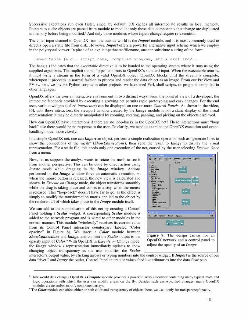
We can add to the sophistication of this net by creating a Control Panel holding a Scalar widget. A corresponding Scalar module is added to the network program and is wired to other modules in the normal manner. This module “wirelessly” receives its current value from its Control Panel interactor counterpart (labeled “Color opacity:” in Figure 8). We insert a Color module between ShowConnections and Image, and connect the Scalar output to the opacity input of Color.9 With OpenDX in Execute on Change mode, the Image window’s representation immediately updates to show changing object transparency as the user modifies the Scalar interactor’s output value, by clicking arrows or typing numbers into the control widget. If Import is the source of our data “river,” and Image the outlet, Control Panel interactor values feed like tributaries into the data-flow path.
8 How would data change? OpenDX’s Compute module provides a powerful array calculator containing many typical math and
logic operations with which the user can modify arrays on the fly. Besides such user-specified changes, many OpenDX modules create and/or modify component arrays.
9 The Color module can affect either or both color and transparency of objects: here, we use it only for transparency/opacity.
Figure 8: The design canvas for an OpenDX network and a control panel to adjust the opacity of an Image.

Supporting Finite Element Analysis with a Relational Database Backend 9
In both cases — direct image interaction and input values via Control Panels — OpenDX handles the events as inputs to the next execution. This is important to understand: you observe, you interact, the result is “looped back,” OpenDX responds, you see the new state. The only difference is that Image manipulations force a new execution. This is a good thing because you should not have to move the mouse away from the Image window to select the “execute” command from a menu each time, then return to rotate the object just a bit more. Control Panel changes do not force a new execution when in Execute Once mode. This permits the user to make changes to several interactors before requesting a new execution using all changed values.
We’ve examined the two most common user interactions within the OpenDX environment. But this report is about interactions between a user, a visualization environment, and a database. We have to create a larger event loop to incorporate new input data from the database. Here’s how it works.
First, let us assume we are starting with a small data set. This means that there is no terrible performance penalty to keeping OpenDX in Execute on Change mode. To fetch different data, say a different subset of grains that meet some changing criterion of interest, the user needs a way to describe the desired data set. A simple approach is to give her minimum and maximum scalar interactors and a menu interactor that permits choosing an attribute field of interest. These parameters, the min and max range, and the field name, are provided as arguments to a Format module which constructs a string from a template, like:
!Python_script.py dbserver database field min max10
This string is fed to Import. Since Execute on Change is selected, when the user changes any of the three input arguments via the Control Panel, Import fires off a new “python executable and arguments” request to the OS and sits back and waits. The Python script constructs a SQL query based on those arguments, calls SQL Server (via ODBC), receives the results, constructs a valid OpenDX object, and returns the stream to Import. Import ingests this DX object, then passes it downstream to the Image module. Result: an image, say with polygonal surfaces colored according to the attribute data that falls within the min-max range specified.11
Figure 9: The Polycrystal Viewer pipeline connects OpenDX and SQL Server via Python (and its ODBC/DBI module). By invoking scripts with UI control generated arguments, OpenDX triggers the dynamic SQL query generation. SQL Server responds with streams of data which are transformed into DX objects by Python scripts.
The user, observing the current image (the result of the preceding execution), decides she wants a larger range, tweaks one of the interactors, and off the whole process goes again. This is key: because OpenDX sees a new argument list, the old data that is cached internally by Import is now seen as out-of-date so a new execution begins, starting at Format, then Import, and on down to Image. If instead of changing the data range, our analyst simply changes the orientation of the view, the new execution caused by releasing the mouse after rotating would only cause Image to re-execute. Rotation does not change Import’s arguments, ergo the cached data is current, so the database would not be called, new data would not be received, and unnecessary operations upstream of Image would not be performed again. Likewise, if the user merely tweaks the opacity of the colored surfaces, only operations at and below the Color module would re-execute.
This internal caching and adaptive re-execution is a two-edged sword. Most of the time, this is an enormous productivity enhancement in an interactive session. If the user happens to reselect the same min and max values, DX will recognize that it holds a cache object matching that specification and will quickly regenerate the resulting image
10 dbserver and database are strings provided by other Control Panel interactors. They generally remain the same for an entire
session. 11 And it generally takes far less time for all that activity than it took you to read this footnote.
Session OpenDX Python
SQL
Data DX Object
Arguments

- 10 -
(no call is issued to Python). But the other edge of the sword is exposed if the database is being dynamically updated. DX would not know the external data had changed, so would show the previously cached data associated with a particular parameter string.12 In our system, we effectively sandbox the user’s access to a particular set of databases for which the contents are static during any user visualization session.
Now that we’ve introduced the concept of (effective) loop-back to an otherwise rigidly top-to-bottom data-flow scheme, we can describe the Pick feature. Like the Scalar module in our previous example, a Pick module is placed on the canvas and wired into the net; it has no initial value until a pick is made. Picking is a direct interaction with the Image window. The user clicks the mouse on any part of the displayed object. A ray, normal to the screen, is “fired” through the object, intersecting each surface the ray passes through. The result is a pick object. We generally prefer to fetch the precise data value associated with an actual mesh vertex rather than an interpolated value from an in-between point. Because our aim is not always true, DX can determine the closest vertex on the actual mesh to the arbitrary intersection point of the ray (a list, if the ray intersects multiple faces). Appendix C: The Initial Grains DX Object shows how “grain ID” data is made dependent on grain positions in Component 5 (attribute “dep” “positions”). Knowing the precise position of the closest vertex, DX recovers the corresponding exact data value. It is this data — the list of grain IDs — we receive from the pick ray we shot through the polycrystal.
As with other Image interactions, picking generates a result that is not available until the next iteration of the DX net. Consider that you must have an object displayed to make a pick, so the execution that first makes the object cannot also contain the result of a pick. Succeeding executions can include both the object and a pick result. Unlike the other transformation operations, Pick’s results are only useful upstream of Image, akin to the way we insert Control Panel values into the data flow. In Execute on Change mode, picking will appear to have immediate results. In the polycrystal viewer, the intersection of the ray with multiple faces returns a list of grain IDs. These numbers are fed back into the net and permit us to make transparent all grains that are not in the pick list, leaving only a “shish kebab” of picked grains (Figure 6).
More than one Pick tool can coexist in a net. Currently, we employ four; each is preset to only “hit” specified scene objects. One is used as just described to return a list of grain IDs. Another is designed to pick subsets of tetrahedra adjacent to grain edges. A third permits the user to select any arbitrary mesh point to become the new center of rotation and scaling — very handy when trying to examine local regions in extreme close-up.
The fourth Pick illustrates a remarkable bit of cooperation between OpenDX and SQL Server. We named this the Histogram_Bar Pick tool. In the polycrystal database, each grain or tetrahedron or mesh triangle may be characterized by more than one descriptive data field. For example, mesh triangles have area, aspect ratio, and alpha (a shape measure). These sorts of measures lend themselves to traditional visualization, i.e., charting. We first added a simple histogram (bar chart) using the Plot module to view any specified range of these measures.
It occurred to us that the bar chart itself could serve as an interactive control. By recomposing the bar chart as a set of quadrilateral connections with dependent data values (the counts or frequencies), we created a new object that can be Pick’ed on. We determined that it was more efficient to manufacture this histogram in SQL Server and return it as a DX object ready for display; it is not a very large stream, so communication time is not an issue. The call looks like:
!Histogram.py dbserver database field number_of_bins chart_min chart_max
Naturally, the user can control the latter four arguments to customize the chart. When the histogram object is displayed, the user simply clicks a bar and the value range for that bar is retrieved and sent via Format, Import, and a different Python script to the database:
!Histogram2Grains.py dbserver database field bar_min bar_max
This returns an object structure containing a mask value of 1 for selected grains, that is, those grains containing elements whose field data lies within the selected bar range, and 0 for unselected grains. Note that the grain ID data is not contained in the bar: it is retrieved indirectly during the database procedure. Thus, we create a visualization of data in which the visual representation itself (the bar chart) carries sufficient information to be employed as a control to affect another visual representation (the 3-D display of the polycrystal). One use is for identifying the physical location of outliers, like tetrahedra or triangles with undesirable aspect ratio (splinters or needles). The analyst
12 There is a menu operation that will reset the cache and force the entire program to execute from scratch, thereby fetching the latest data from the source.
Supporting Finite Element Analysis with a Relational Database Backend 11
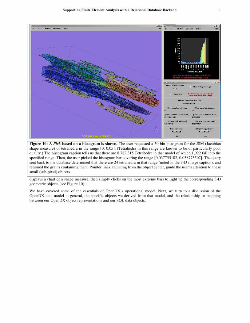
displays a chart of a shape measure, then simply clicks on the most extreme bars to light up the corresponding 3-D geometric objects (see Figure 10).
We have covered some of the essentials of OpenDX’s operational model. Next, we turn to a discussion of the OpenDX data model in general, the specific objects we derived from that model, and the relationship or mapping between our OpenDX object representations and our SQL data objects.
Figure 10: A Pick based on a histogram is shown. The user requested a 50-bin histogram for the JSM (Jacobian shape measure) of tetrahedra in the range [0, 0.05]. (Tetrahedra in this range are known to be of particularly poor quality.) The histogram caption tells us that there are 8,782,315 Tetrahedra in that model of which 1,922 fall into the specified range. Then, the user picked the histogram bar covering the range [0.037755102, 0.038775507]. The query sent back to the database determined that there are 24 tetrahedra in that range (noted in the 3-D image caption), and returned the grains containing them. Pointer lines, radiating from the object center, guide the user’s attention to these small (sub-pixel) objects.

- 12 -
OpenDX Data Model
The fundamental power and longevity of DX (now over a dozen years old) is based on its profoundly well-conceived and implemented data model. Figure 11 shows our formal ontological description of the OpenDX data model. It may help to refer to this when reading the following.
OpenDX and its data model sprang from a careful analysis of how the majority of scientists and engineers organize their data, and the elucidation of the common elements that underlie such data organization. Fundamental to this model is the assumption that we sample data in a topological space, associate the samples with spatial locations, and embed them in a Cartesian space for the purpose of visualizing the arrangement using computer graphics techniques. Measurements are made at discrete times and locations in either discrete or continuous space-time. In continua, we assume that values at other locations and times can be estimated by interpolation paths that join known measurements.
In DX terminology, sample locations are positions, interpolation paths are connections, and sampled values are data. Scattered data (data on unconnected positions) are supported. Regular and irregular mesh topologies are supported as are both regular positions and irregular positions; regular positions and connections permit more efficient use of memory (a luxury not available in our models). 1-, 2-, and 3-dimensional positions are visualizable.13 Scalar and vector14 data, real and complex, of virtually any type (float, int, byte, etc.) may be associated with either positions or connections, and are called position-dependent data and connection-dependent data, respectively.
Positions, connections, and data are keywords for Components, and are bound together in Field objects.15 The Field is the most generally useful basic object as it represents a self-contained visualizable entity. Other Field components of interest include colors, opacities, normals, invalid positions, and invalid connections (the latter two serve as masks).
13 Higher dimension positions are supported, but must be “sliced” to a visualizable dimension to be displayed. 14 A tuple may have many elements, for example, a 3-vector of [i, j, k]. One author has personal experience with manipulating
57-element vector data in DX. 15 For clarity, we’ll capitalize Field when referring to a DX Field Object, in distinction to the general notion of a physical or
mechanical field. Likewise, we’ll capitalize Group, Array, and some other DX keywords where the context might be ambiguous. Other DX keywords will be italicized.
Figure 11: A dictionary of core DX concepts (OWLViz [27]) is shown. At the first level are scalar types, standard DX Objects, and — what we prefer to call — function objects. Function objects are not DX Objects. They are relations between and qualifiers of DX Objects. DX Components are prime examples of function objects. They relate DX Objects to Fields (as their components). DX provides standard templates for Array objects which represent structured positions or connectivity and which are listed under PositionsArray and ConnectionsArray. Standard DX array components are listed under ArrayComponent.

Supporting Finite Element Analysis with a Relational Database Backend 13
Connections over which interpolation may be performed include: lines (1-D topology which may have 1-D, 2-D, or 3-D positions); triangles and quads (planar polygons in 2-D or 3-D space); cubes and tetrahedra (volumetric polyhedra in 3-D space). In addition — and key to our project — DX supports an edges–loops–faces construct to describe arbitrary polygons. We assemble multiple polygonal faces to form the appearance (but not the actual substance) of arbitrary volumetric polyhedra (which do not exist in DX as primitives).16 We also have complete volumetric tetrahedral space-filling meshes for each grain.
Fields can be joined into Groups. Groups may contain other Groups and/or Fields, as well as other esoteric objects such as lights, cameras, and so on. Special-purpose Groups include Series and Multigrid.17 These constrain member type and permit some modules to work over the domain of all members within the Group. For example, the Colormap module can automatically find the minimum and maximum value of the data in an input Field and then generate a colormap that spans the complete range. Likewise, when a Multigrid or Series is fed to Colormap, the module will scan all members and find the joint minimum and maximum of all the data Components. This is usually the desirable range when showing a time series, since the values associated with “blue” and “red” will be fixed throughout the animation.
Groups may be arbitrarily nested hierarchies (sans recursion). We take great advantage of this capability. Appendix C: The Initial Grains DX Object shows the deeply nested structure of the initial object that contains the menu contents for a visualization session with the polycrystal viewer.
Groups, Fields, and Components may each have any number of Attributes. Some of these are required, such as the Attribute that declares which dependency a data Component has (example: attribute “dep” “positions”). User-generated Attributes (“date of measurement,” “instrument model,” etc.) are passed through modules without complaint to be accessed by the Attribute module when needed for a caption or other purpose.
Data-like Components may also have user-provided names (like “aspect ratio,” “alpha,” etc.). Component Arrays may be multi-valued or constant. The ConstantArray is convenient for compactly assigning the same value (like grain ID) to all parts of an object that might be Pick’ed, since anywhere you hit the object, you get the same value.
OpenDX provides a scheme in which a user-defined cache object can be created, retrieved, manipulated, and stored iteratively within the scope of a macro. This serves, in effect, as a “For” loop construct, allowing the programmer to accumulate a sum, append items to a list, etc. However, this routine more than any other in OpenDX exposes the weakness of run-time versus compiled execution. The desirability of using the Get and Set modules decreases as the number of iterations rises; at some point, the wait becomes noticeable (or irritating) to the user. We avoid using this technique, but occasionally, it is the optimal solution to perform a necessary task.
The most efficient DX operations are Group- or Array-oriented. It is much faster to do an operation on all members of a Group or an Array using a precompiled module than to iterate explicitly using Get and Set. When we perform a Group or Array operation, the necessary iteration is part of the compiled module’s code. The programmer writes no explicit iteration code: the “For” loop is implicit. Thus, whenever possible, we try to construct our objects to facilitate such operations.
With this background on OpenDX, we can now describe how we implemented the polycrystal viewer application.
Polycrystal Viewer Implementation Highlights
A polycrystal analysis session works like this. The user can start at either Step 1 or Step 8.
1) User launches PreView (OpenDX program)
• when the DX net executes the first time, the XML file app.config (see Appendix E) is processed by a Python script to generate a DX Object that populates variable menus
• generally, the net is kept in Execute on Change mode and responds to changes as the user makes them
2) Choosing from these menus, the user determines a database
16 One may determine the value at any interpolated point inside an OpenDX cube or tetrahedron connection; the interior of our
arbitrary polyhedral grain is empty. 17 The OpenDX Multigrid does not have a constraint that members abut without gaps or overlap. It serves as a general-purpose
packaging scheme.

- 14 -
3) OpenDX invokes a Python call to SQL • a low-resolution view of a polycrystal is retrieved and displayed • grains are simple cubes rather than arbitrary polyhedra • cubes are scaled proportionately to grain size • cubes may overlap/intersect in this low-res view • cubes have colors based on any user-specified parameter
4) With various techniques, user selects a subset of grains to examine more closely 5) Selection parameters determine additional Python calls to SQL
• new data is fetched, returned, and displayed 6) Steps 2–5 are repeated ad libitum 7) When the user is satisfied, he “commits the session”
• a Python script triggers the creation of a table in the SQL Server tempdb database • the same Python script writes a .dxsession file in the user’s work directory
8) User launches PView (OpenDX program) • XML file app.config is processed by a Python script to generate a DX Object that populates
variable menus • if .dxsession is present, the user can designate that it constrain the work session to the previously
selected grains (those in the tempdb table) • PView displays the full-resolution version of the specified polycrystal or grain subset.
Here are some of the typical operations available to the analyst using PView (see also [18] for a live demonstration of many of these operations).
1) Display an aggregate of polycrystal grains (Figure 5) • smaller databases may be shown completely • larger databases are best first sub-selected with PreView, as their complexity may exceed available
machine resources • Value: observe 3-D grain structure and shape
2) Display a histogram (Figures 2 and 10) • chart any physical field or mesh attribute data • select bin count and specify range of interest • chart becomes a pickable “interactor” (item 7, below) • Value: traditional “big picture” chart-based analysis
3) Isolate grains (Figures 2, 4, 5) • by shrinking their vertices and faces toward each grain’s local “region center” • Value: useful for seeing “inside” the polycrystal
4) Distinguish and display 3 grain sets with a slice plane (Figure 2) • sets are: intersected by, “in front of,” and “behind” the plane • opacity of each set may be varied from fully transparent (hidden) to fully opaque • animate the slice plane over a range along its normal direction • Value: reveal interior structure of the polycrystal
5) Select grains with a slice plane • the grain set intersected by the plane becomes the selected set • in distinction from item 4, this operation also returns additional data needed for intersection (item
12, below) • Value: select a set of adjacent grains over an area
6) Select grains with a pick ray (Figure 6) • the grain set along the ray becomes the selected set • highlight all selected grains • show any single grain on the intersection list • invert the set (show “unselected” grains) • pick ray may be constrained to hit grains within only one of the current slice plane sets (item 4
above) • Value: select a set of adjacent grains along a line
Supporting Finite Element Analysis with a Relational Database Backend 15
7) Select a grain set by histogram bar picking (Figure 10) • highlight the grains that contain field values in the range of any histogram bar • invert the set • Value: explore the polycrystal indirectly by field data selections
8) Select grains by text ID • type in a list of one or more grain IDs • invert the set • Value: provides direct access/return to known IDs
9) Show surface mesh features (Figure 4) • wireframe (triangle edges) • all triangles (as polygons) • triangles within a criterion range for a specified attribute field • triangles within the field range specified by the complete current histogram or the currently picked
histogram bar • Value: search for and inspect badly-formed elements (mesh generation artifacts)
10) Show volumetric features • same choices as for surface mesh, with attribute field types appropriate for tetrahedral volume
elements 11) Display pointer rays (Figure 10)
• rays emanate from the center of the polycrystal bounds box and terminate at the centers of selected triangles or tetrahedra
• Value: highlight very tiny elements which may be invisible at default zoom length 12) Intersect selections
• intersect the current mesh (item 9) or volume selection (item 10) with the current grain selection (items 5–8)
• display only the common elements • Value: reduce complexity of display and focus on correlations
13) Display topological edges • these are elements of the representative polyhedral faces (distinct from the computational mesh
edges) • color edges by edge ID or by junction count (number of faces sharing that edge) • display edge ID labels • select a topological edge to show the tetrahedra in adjacent grains that share that edge
14) Display statistics (Figures 2 and 10) • “number of current triangles,” “IDs of grains currently selected,” and so on
15) Display continuous physical/mechanical fields (Figure 6) • fields are mapped from the FEM to the appropriate geometric elements by SQL Server • user can manipulate colormaps • color is interpolated across surface or volume mesh by OpenDX renderer • Value: displays the results of FEA on either the computational mesh or the representative (face)
objects 16) Animate time step data
• for data sets with “cases” • play flip-book animation over a series • Value: observe temporal change of a parameter
17) Change view point • rotate, pan, zoom, fly • set the point of rotation and center of zoom to any selected feature or to the polycrystal as a whole • Value: enables close inspection of details in 3-D
Let’s talk in detail about a few of these PView operations. First are the general techniques for selecting a set of grains.

- 16 -
Grain Sets (Nos. 4–8)18
Earlier, we described how the analyst makes a selection with the pick ray and histogram bar pick tools. Now, we describe how OpenDX and SQL communicate this information to each other.
When PView is launched, a data set is selected and the parameters are sent via Python to SQL Server. The returned DX object is a Group (Appendix C: The Initial Grains DX Object). This Group contains three members: a Field with the true bounding box of the polycrystal,19 a Field with the bounding box of all vertices in the polycrystal database,20 and a Multigrid containing the geometry and initial data values for each grain. Since each grain Field object is structurally similar, we bundle them into a Multigrid.21 The chief virtue of bundling is that Multigrid members have “grain ID” string identifiers by which we can select subsets. Each Field carries the positions, edges, loops, and faces that permit us to display the grains as (hollow) polyhedra. Each Field also contains Components that hold grain ID, region center (3-vector), and data which identifies each grain’s set membership.
To change the visibility of grains based on a selection, we could ask the database for a new Multigrid of grains, in which each member has the appropriate set membership data. If a grain is selected, this value is 1; if a grain is to be hidden, the value is 0.22 Theoretically, we could substitute the new Multigrid for the initial grains Multigrid since the two objects would have the same structure, member order, and member count. In practice, that would be inefficient.
There are two communication issues here: first, how do we tell SQL Server which grains are selected? And second, isn’t it going to be costly to send all the geometry and face data for grains, over and over again, each time a new selection is made? After all, the only things that change due to a selection are the set membership values.
As to the first point, we promptly discarded the idea of sending a variable-length string list via Python as likely to be fraught with difficulty. Very large polycrystals subjected to arbitrary selections would generate potentially very long character strings. This would almost certainly wreak havoc in the handoff from OpenDX to Python to SQL Server. Instead, our selection routines are designed to send small (no more than a few dozen bytes), fixed size, and clearly defined packages of information to the server. For the slice plane operations (items 4 and 5), the direction of the normal and a point on the plane are sufficient to parameterize a stored procedure that can determine, on the SQL Server, into which set each grain falls. The histogram bar pick needs only send the currently selected field attribute and the minimum and maximum value of the selected bar for SQL to determine which grains contain data in that range.
With regard to the issue of minimizing data transfers, we structured our objects to take advantage of the inherent efficiency of Group-oriented operations. On the first execution of PView , we acquire a full “initial” Multigrid with all the necessary geometry information at a very coarse level of detail. Conveniently, the Replace module permits us to “copy and paste” Components from one object to another, as long as the structures of the objects are compatible. To update all the data Components (one per Field) in the initial object, we discovered that we need only return a “skeletal” Multigrid object from SQL Server: it has to retain the same member count and order of members but each member contains only a single Array. Replace traverses the two objects member by member, and performs a one-to-one substitution overwriting the Arrays in our old data Components in the full Multigrid with the new data Arrays, thereby changing the set membership of each grain as we drill down and refine the level of detail in some regions of the model. The replacing object is illustrated in Appendix D: The Histogram Bar Selected Grains DX Object. The replacement Multigrid is member 0 of the Generic Group; members 1 and 2 contain ID lists used for captions and the intersection routines (item 12 in the operations list above). The new Multigrid always has the same number of members, equal to the number of grains in the initial object. The user controls the display of the 2 or 3 grain sets, and may hide any or all by making their opacity equal to 0.
Selections based on a pickray or text-based ID selections are even easier and are both made entirely on the DX side with no communication to the database. The pick ray passes through the polycrystal object. As it intersects a face of a grain, OpenDX determines the closest actual vertex (found in the grain positions). Since we associated a grain ID with each position in the original Multigrid, that data value is easily recovered. The ray passes through each grain an
18 Nos. refer to items in the immediately preceding operations list. 19 Even if no grains are selected, this box visually indicates the polycrystal’s domain — the valid target area for picking. 20 Some databases may have vertices that are not connected to any face; these probably should be cleaned out, but this box serves
as a diagnostic of their existence. 21 Their structural similarity logically implies — but does not require — the use of a Multigrid. In fact, a Generic Group would
work. 22 In the slice plane display mode (No. 4), the intersected set has value 2, the “behind the plane” set is 1, and the “in front” set is
0.
Supporting Finite Element Analysis with a Relational Database Backend 17
even number of times, entering and exiting more than once if the grain has a complex shape, so the pick ray’s grain ID list will have at least two identical entries. We use the Categorize module to reduce the list to unique grain IDs. For text-based selection, the ID list is taken directly from the dialog box. Recall that each member of the grains Multigrid is identified by its grain ID. When fed the string list of names and the grains Multigrid, the Select module extracts the subset of named members.23
In contrast to the Multigrid Replace scheme, the output of Select is a Multigrid with (generally speaking) fewer members than were in the input. The opacity of the single resulting subset is under user control. Unselected grains are not included in this reduced set, so do not show at all.
To summarize: in some cases we send and receive minimal information, because finding the grain set is more efficient using SQL Server procedures and spatial indices. In other cases, OpenDX provides a fast native scheme to show only selected items without any communication with the database.
Grain Isolation (No. 3)
While OpenDX’s Isolate module can shrink DX-native volumetric objects toward their respective centers, this module does not accept our arbitrary polyhedral grains. To achieve the same effect, we added the region center Component to the initial Multigrid of grains. It is a trivial and efficient Group and Array operation in Compute to scale each vertex along the direction vector from the grain’s region center to the original vertex location, with the expression:
Position_A + (scale_factor * (Region_Center_A – Position_A))
where Position_A is an array of vectors with variable values, Region_Center_A is a constant array with effectively the same vector value at each index, and scale_factor is a single scalar provided by the user via a Control Panel.
Because edges, loops, and faces are all attached to positions by reference (directly or indirectly), they are automatically dragged along to the new locations, retaining the same polyhedral shape.24
This operation is very efficient because DX automatically iterates over each Multigrid member to fetch its data and region center Components, then iterates down these two lists of items to generate the corresponding output list. This doubly-nested iteration is handled entirely by a single Compute, using the expression shown.
This is an example of a routine that we first tried implementing in the database. The user controlled an “isolate factor” Scalar and that value was relayed to SQL Server which calculated and sent back new grain geometry. That was a far more costly approach (communication time and network load) and was abandoned once we thought of the region center solution. It serves, though, to make the larger point that our system has such flexibility that we can pick and choose where best to perform operations, depending on a number of determining factors, such as computational efficiency, communication load, and interactive performance. While our first solution worked, when we began optimizing our overall data-flow, we saw that shipping the small additional region center component at the outset permitted arbitrary resizing of grains with a much smaller total communication cost.
Histogram (No. 2)
The display of a data histogram illustrates the benefits of both SQL Server and OpenDX. It is not feasible to ship all the stored field data for all cases from SQL to OpenDX — that’s why we’re using a database in the first place! The trade-off then becomes whether we send requested data in the form of an array of values or if we send a more structured object. If we send only an array, it would reduce network traffic, but when it arrived, we would have to wrap it in a structure (like a Field) to display it. The structuring work takes a bit of extra time and consumes more memory. After experimenting with both solutions, we chose to return a complete DX Object from SQL. This OpenDX Field object consists of a list of 1-D positions (along the X-axis) spanning the minimum to maximum of the desired range, connected by lines (the number of lines equals the number of bins requested by the user), with the data (counts) mapped to each connection element. OpenDX’s Rubbersheet module extrudes each line segment in the Y direction, proportional to the data, converting our 1-D line into a set of 2-D quadrilaterals (the bars). AutoColor applies a color based on the count for each segment. The AutoAxes module dresses the graph with labels and tick marks. By virtue of being DX objects, the bars may be picked to return information about their individual ranges; we described earlier how this is used by the histogram bar pick routine. This shows a typical division of
23 Select actually ignores duplicate entries, but we also send this list to a menu for the user to select one grain at a time; there,
duplicate entries would be annoying. 24 Shape is retained within limits, especially in the case of complex grain shapes with concavity. Things will get ugly if you
shrink them too far!
- 18 -
labor between SQL and OpenDX. SQL does the subsetting and some basic calculations; OpenDX does all the work needed to render the information.
Physical/Mechanical Field Display (No. 15)
Case studies generate enormous amounts of physical data, far too much to ship to OpenDX before it is requested. In fact, until the user specifically calls for a particular field mapped onto a particular geometry, the data for that mapping may not even explicitly reside in a database table. That is, many physical or mechanical measures inherently “live” on tetrahedral volumetric finite elements within grains. But the user may wish to see that data mapped to the surface mesh of a grain. These values are only computed on demand.
Similar in overall structure to our grains Multigrid, the initial surface mesh Multigrid is a Group of Fields whose connections are triangles (instead of edges, loops, and faces). This mesh is downloaded from the database and displayed when the user requests it. Initially, the data values are simply grain IDs. This is a large object due to all the positions and triangle connections it contains to describe a complex mesh, so we only ship it once.
When a request is received to map physical data to this surface mesh, a SQL Server stored procedure performs the necessary interpolation from volume element-based data to node-based (position-dependent) data. The overall structure of this sparse Multigrid with (only) mapped field data matches the initial surface mesh Multigrid, permitting Replace to efficiently swap the new physical data for the placeholder data.
Intersection of Selections (No. 12)
Triangles and/or tetrahedra may be displayed independently of the current grain selection. Once a grain selection has been made, it can be intersected with either a triangle selection or a tetrahedron selection or both. The intent of intersection is to simplify the display so we can more easily identify the grains that contain certain mesh elements, like triangles with distorted aspect ratios. That permits viewing tiny mesh elements in the larger context of the grains which contain those elements; generally, one would adjust the grain opacity to a semi-transparent setting, turn on the “pointer rays” feature (No. 11), then zoom in for close inspection of the elements at the end of the pointers.
Triangles and tetrahedra are selected in one of three ways: by specifying an attribute and a criterion range for that attribute (such as “triangle aspect ratio” between 0.01 and 0.03); by specifying a histogram field and range; or by selecting a histogram bar, thereby choosing its field and sub-range.
Our DX object description of the selected triangle set is a Group containing a Multigrid with a member for each face. Within each member, a Field holds the geometry and topology for the one or more triangle elements on that face that meet the current selection criteria; if no triangles on a face meet the criteria, the face is excluded from the Multigrid.
The top-level Group also contains an Array that holds the list of unique face IDs in the current selection. There is no efficient way to derive this Array in OpenDX (we would have to iterate over the Multigrid member names), but it is simply done in SQL Server. We decided it was, on balance, more efficient to ship this list instead of building it iteratively in OpenDX.
When we make a grain selection with the histogram pick tool or with the slice plane selector, SQL Server knows which grains are in the “selected” set and it attaches to the replacement object an Array listing these IDs. Appendix D: The Histogram Bar Selected Grains DX Object shows the replacement object structure. It is a Group with three members. The first member is the “skeletal” Multigrid we described above in our discussion of Grain Sets. The latter two members contain the string list of currently selected grains, and the list of all faces on those selected grains. Each list contains only a single reference to each unique value. The object returned from a slice plane selection has the same structure.
In the Grain Sets discussion, we described how a pick ray selection returns a list of unique grain IDs. We have to do a bit more work to generate the unique face list for a pick ray selection. Since we do not communicate with SQL Server, we have to accomplish this in OpenDX, and this requires Get-Set iteration. (Figure 12) For each grain in the Multigrid, we extract its face ID Component (face ids str in Appendix C: The Initial Grains DX Object) and build one list from these input Arrays.25 Once we have that combined list object, we resume efficient native DX operations and Categorize the unique face ID list.
25 The number of iterations equals the number of grains in the input list. A pick ray will contain O(n1/3) items, where n is the
number of grains in a roughly cubic polycrystal. We decided this would not be onerous for n � 105.

Supporting Finite Element Analysis with a Relational Database Backend 19
At this point, we have a grain selection and the face list on those grains, and a triangle selection and the face list containing those triangles. How do we intersect these different kinds of objects?
To intersect the triangles object with the grains object, we simply Extract the face IDs Arrays from each object and append one list to the other. We know in advance that each list contains only one reference to any particular face ID. This joint list is then run through Categorize to build a lookup table of face IDs in the joint list. CategoryStatistics returns a count of the number of occurrences of each unique face ID. If there is only one occurrence, that face ID only occurs in one list or the other, so we eliminate it. If there are two, we know that face must occur in both lists, so we include it in the list of faces to Select from the faces Multigrid for display.
Intersecting tetrahedra is similar but we use the grain ID lists provided in each object to build our joint list. We don’t need to iterate, since we already have a complete unique grain ID list regardless of selection method.
To close our discussion of visualization techniques, we illustrate the iterative macro that builds the list of faces. The OpenDX networks are shown in Figures 12 and 13. The point of this illustration is to point out the lone case where “circular logic” (or “data running uphill” if you like) is permitted in OpenDX. The right-hand connection from SetLocal to GetLocal shows that they share a common cache object, here the growing list of face ID values. On entry into this macro, GetLocal has a null value. On each iteration, the data (list of face IDs) from the next member of the input Multigrid is appended within List, then stored in the cache, for retrieval on the next iteration. After all input items are processed, the complete list is emitted from the macro’s output. The macro is shown as it appears in a net, in Figure 13 below.
Figure 12. An iteration macro (BuildListFromMultigrid)
Figure 13. The BuildListFromMultigrid used in a network program
CAVE
We already discussed visualization techniques to limit view complexity. An immersive projection environment can increase the richness of what we are able to comprehend visually by providing more pixels, by providing 3-D, and by providing a wrap-around visual space. Immersive environments aid distance perception in two main ways: stereoscopic view by showing separate images for the left and right eyes, and motion parallax by changing the display as the viewer’s head moves. Complicated geometry is easier to understand in stereo on a desktop or in a fully immersive environment.
Rewriting the visualization application to run immersively was not an option – that would be too much work. There are several visualization packages, similar to OpenDX, which run either on the desktop or completely in a CAVE, meaning that every menu, dialog box, and window appears within the immersive environment where the user can change values and manipulate the simulation (AmiraVR, COVISE [32].) We determined that a simple extension to OpenDX would give us both stereo display on the desktop and immersive display in the CAVE without significant modifications to the DX net.
- 20 -
We wrote an extension module for OpenDX which sends geometry over the network to client applications. We then wrote two client applications, one to show stereo images on the desktop and one to run immersively in the CAVE. The result is that a researcher with a Tablet PC can walk into the CAVE, load an OpenDX visualization on the tablet, and fly through it immediately using the CAVE wand controller.26 Because we need to enter numbers and navigate the quite complicated DX net, a hybrid solution using both the Tablet PC for net manipulation and typical CAVE controllers for exploring the resulting model works quite well.
The CAVE program is written in SGI Performer for Windows. It talks with OpenDX using .NET27 Remoting or sockets. A disadvantage of sending the model across the network every time the DX net changes is that each change to a model initiates a transfer to the CAVE of all the model structure, which can take up to a few seconds. While this seems quick, it is too slow for smooth movies. We may be able to use caching mechanisms in the future to enable the CAVE program to show movies as smoothly as OpenDX on a local client.
OpenDX for Windows
OpenDX was originally developed by IBM as the IBM Visualization Data Explorer (DX) product supported on IBM’s Power Visualization Server (PVS), SP series of supercomputers, and on a variety of UNIX Workstations. IBM open-sourced the software in 1998 as OpenDX. Since then the open source community has provided support and new development. Microsoft recently funded the enhancements described below.
The DX/OpenDX software package originally consisted of two major parts — an Execution Environment that interprets visualization programs and produces visual displays, and a Visual Programming Environment that supports creation of visual programs through an intuitive drag-and-drop and connect-inputs-to-outputs style. The code in both of these parts utilized a sophisticated (and complex) multi-process architecture, drawing on elements of UNIX process structure and on X11 client/server communication. OpenDX windowing and window management are based on X11/Motif, for the most part using fairly basic windowing primitives, rather than the higher level windowing libraries which are more common today. Though this structure has aged quite well over the years since its original development, it is clearly time to update the architecture to match current technologies and demands.
Since 2002, Microsoft has funded a major overhaul of OpenDX, to eliminate platform dependencies via a system independent core, then add comparable but separate code threads that support both a UNIX-native and a new Windows-native implementation. One benefit of this work will be that OpenDX is available using native Windows capabilities — with consequent performance benefits. A less obvious but very significant aspect of the work is a cleanup of the common core code, ranging from its windowing to process management, which should provide benefits to UNIX and Windows users, as well as to those in the open-source community who are working to extend the code. Because this overhaul affects the base architecture, it has been a major project with the potential to “touch” virtually every line of code in the system. It is now nearing successful completion, and the new code should be released soon [31].
To help describe what is new and better, it is helpful to describe the OpenDX overhaul in a bit more detail. There are two key aspects in revising the code. The first step is to develop a basic, system-independent strategy for inter-process communication — something that will work for both UNIX/X11 and for Windows. This is then applied to produce a common core, with separate UNIX/X11 and Windows threads from that core. The second step is to develop a basic, system independent strategy for windowing — something that will work for both X11 and Windows. Again, this has to be applied to produce a common core, with separate UNIX/X11 and Windows threads.
With this as the basic strategy, work started first on the Execution Environment. The work went as planned, and produced the common core, UNIX thread, and a new native Windows code thread. The changes required in the core were few but significant. The changes were (for the most part) transparent in the UNIX environment. And for the first time a version of the Execution Environment was available that executed on Windows systems. Prior to this there had been a version of OpenDX available that had some internal “tweaks” to patch the process management and used an X11 emulator to manage the windowing on Windows systems. The new version of the OpenDX Execution Environment has redesigned process management to utilize Windows process management capabilities, and more
26 A wand controller is a hand-held pointing device (“virtual stick”) commonly used to navigate and manipulate immersive
spaces. 27 .NET is a Microsoft coinage of recent vintage. DX has called its programs “nets” and saved them with the suffix “.net” since
1991.

Supporting Finite Element Analysis with a Relational Database Backend 21
importantly now displays OpenGL and non-OpenGL native graphics windows without requiring any X-Windows emulation. This version has been widely distributed over the last 18 months and has proven to be very robust [31].
The second step of the project was to create a comparable native executable for the Visual Programming Environment (VPE). Due to major differences between the two windowing paradigms, X11 code (particularly its process management features) could not simply be mapped directly to comparable Windows constructs. Instead protocols were developed to translate X-based “patterns” to comparable Windows-based patterns. These include the following.
• For window manipulation, we developed a “proof of concept” version of the UI under which the core code, minus X11/Motif dependencies, pops up a Windows Forms-based wrapper VPE which loads visual programs, executes them, and displays the resultant image within an Image window.
• For the complex X11 process-to-process and client/server dependencies, threads now communicate with sockets instead of using X11 client/server calls. Communication between graphic windows is passed across threads. The VPE is integrated with the Executive by recasting the Executive as a thread instead of a separate process. The major changes occur within the VPE code. Very little of the core Executive code has to change from the original UNIX-based renderer.
• To promote additional development, we developed a simple C# application to show users how to interact with the new threaded executive. This also helps illustrate our vision for how the UI should be redesigned.
At this time, the entire VPE is being rewritten to use Microsoft's C# programming language, retaining the original structure wherever possible but also recreating key parts of the system to better match with Windows windowing capabilities. We have recreated C# versions of the key base classes of the UI. What remains is to push this process through the entire system, collect and test the parts, and prepare the system for public distribution.
Practical Considerations
For scalability, the polycrystal viewer actually consists of two DX applications, the previewer called PreView and the actual viewer called PView. The previewer is mainly a navigation aid, allowing the user to quickly identify a grain subset of interest, and it operates at reduced geometric resolution (grains rendered as boxes). Typical selections for subsets include the grains contained in box-shaped or spherical probes, grains hit by pick rays, grains intersected by slice planes, or all surface grains. Such a subset can then be further explored at the full geometric resolution in the main viewer. The previewer and the viewer do not communicate directly, but via a “session” table in the database. In session mode PView uses this table to factor out subquery requests.
When opening the Windows Task Manager, a user running PView will notice four key players competing for local CPU and RAM resources: dxexec.exe (DX Executive), dxui.exe (DX User Interface), python.exe, and exceed.exe (X Windows and OpenGL rendering). OpenDX is not noted for its small memory footprint so having plenty of RAM is important. For PView, 2 GB of RAM is the recommended minimum on 32-bit systems. Generally, we have seen better performance on systems with multiple CPUs or CPUs which support Hyperthreading. We did some experiments with multi-threaded versions of the Python scripts, multiple connections, and query re-ordering. We found that performance improved by 10-40% on slow Internet connections; likewise, performance was enhanced on true SMP systems (no Hyperthreading). In our experiments, the physical network (100 Mbit/s Ethernet or better) has virtually never been a bottleneck. With a few exceptions, in the application design we tried to limit the traffic across the network as much as possible and favored data processing (like interpolation) on the server, especially when it resulted in a traffic reduction.
The amount of data in a polycrystal model largely depends on the geometric complexity of the model. The complexity can be quantified to some extent by considering orders of magnitude for object counts like the ones listed in Table 1.
Faces per Grain Vertices per Loop Triangles per Face Tetrahedra per Region
Type 1 101 100 101 103
Type 2 101 100 102 103
Type 3 102 101 102 104

- 22 -
Table 1: Orders of magnitude for object counts.
The scatter for a particular model can be considerable: we have seen models which had grains with as many as 328,000 and as few as 15 tetrahedra in the same model. (Particles, which we haven’t discussed in this report, amplify this effect even further.)
The topological decomposition of a polycrystal into vertices, loops, and faces is the backbone of any visualization using PView and is loaded at startup. A description of the underlying DX object can be found in Appendix C. At its heart is a DX Multigrid with as many members as there are grains in the model. Each member in turn contains Arrays for positions, edges, loops, and faces. What comes across the wire from the database is not the DX object; it is assembled by a Python script. Besides adding the right keywords, it has to renumber all objects, since DX positions are assumed to start at 0 (within each member!) and to be contiguous.28 For not particularly small models (>50 grains) that can take longer than transferring the raw data! Depending on its type, say for a 1000-grain model, the size of the corresponding DX object varies between 2 and 15 MB (ASCII). Another basic object which is important for rendering physical data is the surface mesh. For a 1000-grain model, a surface mesh has roughly 105–106 triangles. Ignoring the vertex positions, each triangle accounts for 16 bytes (triangle ID + 3 corner ID integers). However, the associated DX object is more than twice the total size. Since each grain has its “own” surface mesh there are two copies of each triangle (except the ones owned by external topological faces). In terms of the above example (1 M triangles), this translates into about 40 MB and a few seconds across a Fast Ethernet connection. Again, the renumbering is the bottleneck and takes about twice as long as the transfer across the network. Because of the “Replace trick,” which is described in the section on implementation highlights, the load of the topological decomposition and the surface mesh is a one-time cost. Switching to a binary format and tasking the database server with the renumbering will result in a speedier startup and take a load off the client CPU.
Towards Visual SQL
“The translation of one language into another is not a process of translating each proposition of the one into a proposition of the other, but only the constituent parts of propositions are translated.” (Wittgenstein [30], 4.025)
Although we have been quite successful in meeting the requirements set out for the polycrystal visualization, the design we finally arrived at is far from exhausting what is feasible with today’s commodity hardware and software and it required a substantial effort of various domain experts. What is worse, we effectively did what Wittgenstein suggests is the wrong way to translate the problem — we laboriously translated the concepts more or less one-for-one. The more general question we are trying to answer is this: what is our vision for a system in which a single researcher or engineer could obtain comparable results, a more customized solution, in a matter of a few days?
Even today, the interaction between scientists and visualization experts looks frequently as described in [2]: “Visualization experts are often called upon to help scientists to import and visualize their data. The scientists may not be able to completely (or even consistently) describe how their data set is organized, but the information may be available, embedded inside the data file.” (Chapter 6, page 92). Very much to the point, the chapter is entitled “Mystery Data.” It contains a description of a nifty little tool — the DX Data Prompter — which allows a user to examine the data stored in a file and gather additional information needed to produce a rudimentary visualization. The simplicity of a Q&A type interface to create visualizations is certainly intriguing, but has its clear limitations when it is solely based on files and not augmented by additional domain knowledge.
The development of the original desktop version of PView went roughly as follows: there was an extensive exploratory phase during which we probed different targets in the DX data model to map the polycrystal models onto. (At that point, the polycrystal models were already stored in SQL Server 2000 databases.) Once we had a satisfactory solution the remaining activities consisted of the following:
• Adding new features
• Programming around deficiencies in the DX event handling and UI programming
• SQL optimizations (indexing, user-defined functions)
• Plumbing (Python, XML)
28 The correct thing to do is to push the renumbering, which is nothing but a join with a lookup table, back onto the server. The lookup tables can be generated as part of the general initialization after bulk loading the model.

Supporting Finite Element Analysis with a Relational Database Backend 23
We can certainly think of quite a few cosmetic changes to both database interfaces and visualization tools, which would have made our job a lot easier. For example, having a DX database module or a way to embed SQL into Python would be neat. With the .NET integration into SQL Server 2005 [4], it would be fairly straightforward to build some kind of a “DX shell” into SQL Server. We call these changes “cosmetic” not because we want to suggest they are easily made, but because they do not fundamentally change the way we’ve done visualization so far.
In a more abstract sense, creating a visualization of a scientific or engineering domain (like metallic polycrystals) means to translate or mimic concepts of the application domain ontology [24,25,25] in the visual domain (visual language [22]) and vice versa. In practice, the main impediment in this mapping or coupling process are mystery data — the absence of an explicit and/or formalized representation of a domain’s ontology, including its data model. The database schema is an example of a data model — a file format is not! A populated database — an instantiated schema, — stores facts about objects and the relational calculus can be used to derive new facts. SQL is quite exceptional in that in addition to a data definition language brings with it an “ontology engine” through the relational calculus. However, more general ontology frameworks are necessary (not all data sets live in databases!) and can be defined, for example, in the Web Ontology Language (OWL) [25] and instances can be defined using a framework like the Resource Description Framework (RDF) [24]. Given descriptions of both the application data model and the visualization data model plus an interpretation — a user provided coupling of base objects — a compiler-like generator should be capable of creating mappings to the respective back ends (e.g., SQL queries, DX objects) and synthesize an (initial) custom visualization application.
Summary
This concludes the trio of articles describing an FEA system with an off-the-shelf visualization system and a database backend. The first article laid out the requirements for a modern Finite Element Analysis system. It argued that one needs an integrated system to design the model, create the mesh, run and steer the simulation, manage the data outputs of each of these steps, and then manage the visualization and analysis of the resulting data. The second article described how we mapped the data management problem onto a modern relational database system, Microsoft SQL Server 2005, and discussed the benefits and limitations of that approach. This article discussed the actual analysis of the resulting simulation data and the use of an off-the-shelf visualization system OpenDX. It showed OpenDX lets us interactively analyze a multi-terabyte database resulting from a week-long simulation run. This system has been deployed and is being used by a dozen people at Cornell and in the SIPS project.
We believe our experience with FEA of polycrystalline metals has broader applicability. Most of the FEA simulations we see seem to have similar data management and visualization problems. It seems likely that the techniques described here could be applied in other disciplines.

- 24 -
Acknowledgements
We gratefully acknowledge the support of the Cornell Theory Center, DARPA, Microsoft, Microsoft Research, and Northrop Grumman. We would like to thank the following researchers for providing microstructure modelers and data sets: Anthony R. Ingraffea and the Cornell Fracture Group, Anthony D. Rollett and Steve Sintay of Carnegie Mellon University, and Antoinette Maniatty and David Littlewood of the Rensselaer Polytechnic Institute.
References
1. http://www.opendx.org 2. Thompson, D., Braun, J., Ford, R.: OpenDX – Paths to Visualization. Visualization and Imagery Solutions, Inc. (2001) 3. Heber, G., Gray, J.: Supporting Finite Element Analysis with a Relational Database Backend – Part I. Microsoft
Research Technical Report, MSR-TR-2005-49 (2005) 4. Heber, G., Gray, J.: Supporting Finite Element Analysis with a Relational Database Backend – Part II. To appear. 5. http://www.microsoft.com/sql 6. Butler, D.M., Bryson, S.: Vector-bundle classes form powerful tool for scientific visualization. Comput. Phys. 6 (6)
576-584 (1991) 7. Butler, D.M., Pendley, M.H.: A visualization model based on the mathematics of fiber bundles. Comput. Phys. 3 (5)
45-51 (1989) 8. Daconta, M.C., Obrst, L.J., Smith, K.T: The Semantic Web. ISBN: 0-471-43257-1, Wiley Publishing (2003) 9. Passin, T.B.: Explorer’s Guide to the Semantic Web. ISBN: 1-932394-20-6, Manning Publications (2004) 10. Haber, R., Lucas, B., Collins, N.: A data model for scientific visualization with provision for regular and irregular
grids. Proceedings of the 2nd conference on Visualization '91 , IEEE (1991) 11. Howe, B., Maier, D., Baptista, A.: A Language for Spatial Data Manipulation. Journal of Environmental Informatics 2
(2) 23-37 (2003) 12. Kochevar, P., Ahmed, Z., Shade, J., Sharp, C.: Bridging the gap between visualization and data management: a simple
visualization management system. Proceedings of the 4th conference on Visualization '93, IEEE (1993) 13. Kochevar, P.: Database Management for Data Visualization. Technical Report 94/40, University of California,
Berkeley (1994) 14. Zeiler, M.: Modeling Our World – The ESRI Guide to Geodatabase Design. ISBN: 1-879102-62-5, ESRI Press (1999) 15. Lucas, B., Abram, G.D., Collins, N.S., Epstein, D.A., Gresh, D.L., McAuliffe, K.P.: An architecture for a scientific
visualization system. Proceedings of the 3rd conference on Visualization '92, IEEE (1992) 16. Treinish, L.A.: A function-based data model for visualization. In Proceedings of IEEE Visualization (1999) 17. Zomorodian, A.J.: Topology for Computing. ISBN: 0-521-83666-2, Cambridge University Press (2005) 18. The Cornell Fracture Group Polycrystal Viewer – A video prepared by Chris Pelkie, Cornell Theory Center (2004) 19. http://www.python.org 20. http://activestate.com/Products/ActivePython/ 21. Pilgrim, M.: Dive Into Python. Apress, ISBN: 1-59059-356-1 (2004) 22. Chang, S.-K., Ichikawa, T., Ligomenides, P.A.: Visual Languages. ISBN: 0-306-42350-2, Plenum Press (1989) 23. Cavalcante-Neto, J.B. et. al.: An Algorithm for Three-Dimensional Mesh Generation for Arbitrary Regions with
Cracks. Eng. Comput. (Lond.) 17(1): 75-91 (2001) 24. Powers, S.: Practical RDF. ISBN: 0-596-00263-7, O’Reilly (2003) 25. Web Ontology Language OWL/W3C Semantic Web Activity 26. Date, C.J.: The Database Relational Model: A Retrospective Review and Analysis: A Historical Account and
Assessment of E. F. Codd’s Contribution to the field of Database Technology. ISBN: 0-201-612941, Addison-Wesley (2000)
27. The Protégé Ontology Editor and Knowledge Acquisition System, Stanford Medical Informatics (2005) 28. SWOOP — Hypermedia-based OWL Ontology Browser and Editor (2005) 29. Lacy, L.W.: OWL: Representing Information Using the Web Ontology Language. ISBN: 1-4120-3448-5, Trafford
(2005) 30. Wittgenstein, L.: Tractatus Logico-Philosophicus. Translated by C. K. Ogden, ISBN: 0-7607-5235-4, Barnes & Noble
Books (2003) 31. http://www.opendx.org/developer.html 32. http://www.hlrs.de/organization/vis/covise/
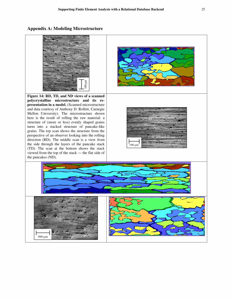
Supporting Finite Element Analysis with a Relational Database Backend 25
Appendix A: Modeling Microstructure
Figure 14: RD, TD, and ND views of a scanned polycrystalline microstructure and its re-presentation in a model. (Scanned microstructure and data courtesy of Anthony D. Rollett, Carnegie Mellon University). The microstructure shown here is the result of rolling the raw material: a structure of (more or less) evenly shaped grains turns into a stacked structure of pancake-like grains. The top scan shows the structure from the perspective of an observer looking into the rolling direction (RD). The middle scan is a view from the side through the layers of the pancake stack (TD). The scan at the bottom shows the stack viewed from the top of the stack — the flat side of the pancakes (ND).

- 26 -
Appendix B: The Menu Initialization DX Object

Supporting Finite Element Analysis with a Relational Database Backend 27
Appendix C: The Initial Grains DX Object

- 28 -
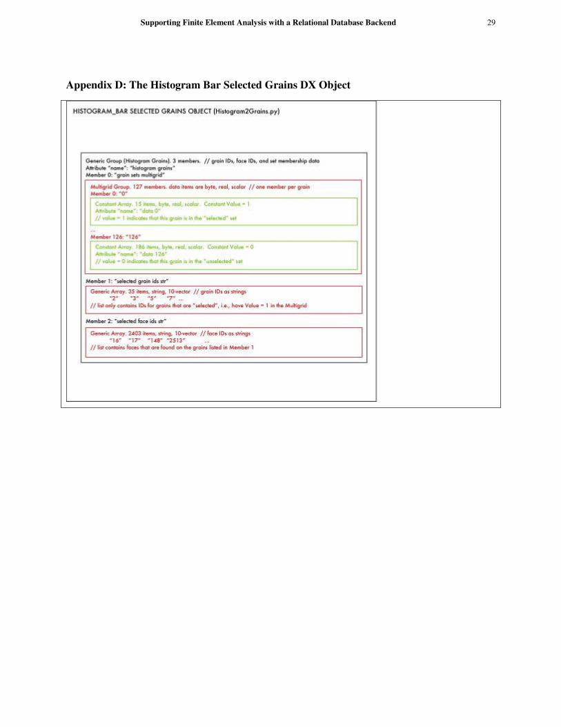
Supporting Finite Element Analysis with a Relational Database Backend 29
Appendix D: The Histogram Bar Selected Grains DX Object

- 30 -
Appendix E: The Structure of app.config
<?xml version=’1.0’ encoding=’UTF-8’?>
<appSettings>
<server name=’server1’>
<db name=’model1’ />
<db name=’model2’ hasVolumeMesh=’true’ />
</server>
<server name=’server2’>
<db name=’model3’ hasMechanics=’true’>
<Case id=’4711’ steps=’0 12 25 34 55’ hasFCC=’true’ />
</db>
</server>
</appSettings>
This configuration file informs the PreView and PView applications (via the menu initialization DX object described in Appendix B) about models’ features and lets them customize the menus on the various control panels accordingly. Database server server1 hosts models model1 and model2. Since no further attributes are provided, the applications will assume that only the unmeshed topological decomposition of a polycrystal is available. When model1 is the current model, the set of fields for which a histogram can be generated will automatically be limited to an appropriate subset and, for example, an option for plotting the area distribution for surface triangles will not be available. Switching to model2 will enable this option, since the hasVolumeMesh attribute indicates that, in addition to a surface mesh, there is actually a volume mesh stored as part of the model. The server called server2 hosts a database called model3 for which an FEA was performed, as indicated by the hasMechanics attribute. The database contains results (e.g., displacement and stress fields) for a case with the id 4711 and at least steps 0, 12, 25, 34, 55 (there could be more). The hasFCC attribute indicates that the model was run with an FCC plasticity material model which triggers DX to provide additional options (plastic slip, etc.) among the features that can be explored. Although it can be generated manually, app.config is typically generated by a Python script which, given a list of servers and models, gathers all relevant information (features) from the databases.


![Finite Element Analysis[May2014]](https://img.dokumen.tips/doc/110x75/55cf921c550346f57b93a5d9/finite-element-analysismay2014-5612ce55d2a43.jpg)


