SUPPLEMENTARY MATERIAL FOR

“Infinite-Dimensional Kalman Filtering Approach

to Spatio-Temporal Gaussian Process Regression”

1 Introduction

1.1 Wiener Process and White Noise

In the actual paper, we have denoted stochastic differential equations in Itonotation (cf. Karatzas and Shreve, 1991; Øksendal, 2003) such as

df(t) = Af(t) dt+ L dW(t), (1)

where W(t) is a Wiener process (or Brownian motion) with diffusion matrixQc. The Wiener process is a Gaussian process with statistics:

E[W(t)] = 0

E[W(t)WT (s)] = Qc min (s, t) .(2)

In this supplementary material we will rewrite the equation (1) in differentialequation form:

df(t)/dt = Af(t) + Lw(t), (3)

where the driving process w(t) is a Gaussian white noise with statistics

E[w(t)] = 0

E[w(t)wT (s)] = Qc δ(s− t),(4)

and can be considered as the formal derivative of Wiener process w(t) =dW(t)/dt. Here Qc is called the spectral density of the white noise process.The space-time white noise can be defined in analogous manner.

The white noise notation is very convenient in practical computations, be-cause in many cases the differential equations can be treated as if they weredeterministic differential equations. For this reason this notation is often pre-ferred in engineering literature (cf. Jazwinski, 1970; Grewal and Andrews, 2001).However, it is important to make sure that every operation is indeed valid inrigorous Ito calculus sense (Karatzas and Shreve, 1991; Øksendal, 2003), andtreat the white noise notation only as a convenient notation for the actual Ito

1

calculus in operation. To emphasis the actual meaning of the equations, wehave chosen to use the Ito notation in the paper itself.

The background of the notation is that in rigorous sense, we cannot directlydefine differential equations driven by a white noise such as (3). Let’s formallyintegrate the equation (3), which gives an integral equation of the form

f(t)− f(t0) =

∫ t

t0

Af(t) dt+

∫ t

t0

Lw(t) dt. (5)

Now the last integral cannot be defined as Riemann integral, because the whitenoise process is formally non-continuous everywhere. However, it can be de-fined as so called Ito stochastic integral (see, e.g. Karatzas and Shreve, 1991;Øksendal, 2003) provided that we interpret the term w(t) dt as increment ofWiener process W(t). In Ito formalism the equation can be written in form

f(t)− f(t0) =

∫ t

t0

Af(t) dt+

∫ t

t0

L dW, (6)

where dW is the Wiener process increment. The second integral is now stochas-tic integral with respect to the stochastic “measure” W(t), the Wiener process.If we drop the integral signs and consider small values of t− t0, the equation canbe written in the more compact form (1), which is the most common notationfor Ito stochastic differential equations in stochastics literature. The solutionf(t) of an Ito stochastic differential equation is called an Ito process. Note thatthe equation can be formally written as

df(t)/dt = Af(t) + L dW/dt, (7)

and comparing to Equation (3) reveals that the white noise process can be con-sidered as the formal derivative of Wiener process dW/dt. However, a slightlyproblematic thing is that the Wiener process is everywhere non-differentiable,and this causes appearance of the delta function in the covariance of white noise.

For the above reasons we also use the Ito notation for infinite-dimensionalstochastic differential equations in the actual paper, because there the situationis analogous to the finite-dimensional case. In this supplement we use the whitenoise notation, because it is easier when doing the actual analytic calculations.

1.2 Multi-Dimensional Fourier Transform

The Fourier transform of function f(x) : Rd 7→ R is here defined as

F [f ](ω) =

∫

Rd

f(x) exp(−iωT x) dx. (8)

The inverse transform is

F−1[F ](x) =1

(2π)d

∫

Rd

F (ω) exp(iωT x) dω. (9)

2

where F (ω) = F [f ](ω). Fourier transforms are rarely explicitly computed,but precomputed tables are often used instead (see, e.g. Rade and Wester-gren, 2004). One-dimensional Fourier transform pairs have been extensivelytabulated in literature and because exp(±iωT x) =

∏

j exp(±iωj xj) multi-dimensional Fourier transforms can be computed as sequential application ofsingle-dimensional transforms. The Fourier transform of a vector valued func-tion can be computed by applying Fourier transform to each of the componentsof the vector separately.

The important properties, which make Fourier transform particularly usefulfor solving linear ordinary and partial differential equations are the following:

• Linearity: If f(x) and g(x) are arbitrary functions and a, b ∈ R are con-stants, then:

F [a f + b g] = aF [f ] + bF [g]. (10)

• Derivative: If f(x) is a k times differentiable function, defined on wholespace Rd and vanishing at infinity, then the Fourier transform of the partialderivative ∂kf/∂xk

i is

F [∂kf/∂xki ] = (iωi)

k F [f ]. (11)

That is, the Fourier transform maps derivatives to polynomials and thustransforms ordinary and partial differential equations into algebraic equa-tions.

• Convolution: The convolution of functions f(x) and g(x) defined on wholespace R

d as above can be defined as

(f ∗ g)(x) =∫

Rd

f(x− x′) g(x′) dx′. (12)

The Fourier transform of the convolution is then the product of Fouriertransforms of f and g:

F [f ∗ g] = F [f ]F [g]. (13)

The Fourier transform is also useful in computing the covariance functions ofstochastic ordinary and partial differential equations due to the following prop-erties:

• Wiener-Khinchin: If f(x) is a zero mean wide sense stationary randomfield with covariance function

Cf (u) = E[f(x) f(x+ u)], (14)

then the spectral density Sf (ω) of the process f(x) is the Fourier transformof Cf (u):

Sf (ω) = F [Cf ]. (15)

3

• If h(x) is a function and H(iω) is Fourier transform (i.e., the transferfunction), then the spectral density of the convolution process g(x) =h(x) ∗ f(x) is

Sg(ω) = H(iω)Sf (ω)H(−iω) = |H(iω)|2 Sf (ω). (16)

The Gaussian spatial white noise process can be defined as a random field w(x)with the properties:

E[w(x)] = 0

E[w(x)w(x+ u)] = q δ(u).(17)

The spectral density of the white noise process can be obtained as the Fouriertransform of the covariance function Cw(u) = q δ(u) and it is given as

Sw(ω) = q. (18)

Due to this property the parameter q or its matrix equivalent in the definitionof white noise is often called the spectral density of the white noise process.

In this document and in the paper write we stationary covariance functionC(x,x′) = C(x−x′) simply as C(x). In the case of spatio-temporal covariances,the stationary covariance functions are denoted as C(x, t).

2 Details of Squared Exponential Covariance Func-

tion Example

The squared exponential (or exponential of square) class of covariance functionshas the form

C(x) = exp(−αx2

), (19)

where in the parameterization of Rasmussen and Williams (2006) we have α =1/(2L2). If we rename one of the input as t, and use separate scales for timeand input, we get

C(x, t) = exp(−αx x

2 − αt t2)

= exp(−αx x

2)exp

(−αt t

2) (20)

which can be seen to be separable in space and time. The corresponding spectraldensity is also separable

S(ωx, ωt) =

(π

αx

)d/2

exp

(

− ω2x

4αx

) (π

αt

)1/2

exp

(

− ω2t

4αt

)

(21)

Following the procedure presented by Hartikainen and Sarkka (2010) we cannow approximate the last term with a polynomial in ω2

t :

exp

(

− ω2t

4αt

)

≈ 1

a0 + a1 (iωt)2 + · · ·+ aN (iω)2N. (22)

4

We can then form the spectral factorization, which will gives

1

a0 + a1 (iωt)2 + · · ·+ aN (iω)2N

=

(1

b0 + b1 (iωt) + · · ·+ bN (iωt)N

)

︸ ︷︷ ︸

Ht(iωt)

(1

b0 + b1 (−iωt) + · · ·+ bN (−iωt)N

)

︸ ︷︷ ︸

Ht(−iωt)

(23)

where Ht(iωt) has poles only in the upper half plane. Thus we get the approx-imation

S(ωx, ωt) ≈ S(ωx, ωt) = |Ht(iωt)|2 Sx(ωx), (24)

where

Sx(ωx) =

(π

αx

)d/2(π

αt

)1/2

exp

(

− ω2x

4αx

)

. (25)

Let ωx be fixed and consider the process f satisfying the stochastic differentialequation

b0 f(ωx, t) + b1∂f(ωx, t)

∂t+ · · ·+ bN

∂N f(ωx, t)

∂tN= w(ωx, t), (26)

where t 7→ w(ωx, t) is a white noise process with spectral density Sx(ωx). Theprocess now has the spectral density, which was defined in the Equation (24).Taking inverse Fourier transform with respect to the space then implies thatthe process satisfying the stochastic equation

b0 f(x, t) + b1∂f(x, t)

∂t+ · · ·+ bN

∂Nf(x, t)

∂tN= w(x, t), (27)

where w(x, t) is a time-white process with spatial spectral density (25), andthus exponential covariance function, has the spectral density (24) and thusapproximately the covariance function (20).

If we define f = (f, ∂f/∂t, . . . , ∂N−1f/∂tN−1), it is easy to see that theabove equation can be written in form

∂f(x, t)

∂t= Af(x, t) + Lw(x, t) (28)

where A and L are constant matrices.

3 Details of the Cressie & Huang Example

Consider the stationary covariance function introduced in Example 1 of Cressieand Huang (1999):

C(x, t) =σ2

(a2t2 + 1)d/2exp

(

− b2||x||2a2t2 + 1

)

. (29)

5

The spectral density is Gaussian in space and thus we get the spatial Fouriertransform easily:

Fx[C(x, t)] =σ2πd/2

bdexp

(

−a2t2 + 1

4b2||ωx||2

)

=σ2πd/2

bdexp

(

−||ωx||24b2

)

exp

(

−a2||ωx||24b2

t2)

.

(30)

Taking Fourier transform with respect to t is again a Gaussian transform forthe last term, which gives the spectral density

S(ωx, ωt) =σ2πd/2

bdexp

(

−||ωx||24b2

)(2b π1/2

a ||ωx||

)

exp

(

− b2

a2||ωx||2ω2t

)

=2σ2π(d+1)/2

a ||ωx|| bd−1exp

(

−||ωx||24b2

)

exp

(

− b2

a2||ωx||2ω2t

)

.

(31)

Let’s form the following Taylor series approximation to the inverse of the lastterm, write it in terms of iωt and factor out the highest order term:

exp

(b2

a2||ωx||2ω2t

)

≈ 1 +

(b2

a2||ωx||2)

ω2t +

1

2

(b2

a2||ωx||2)2

ω4t

= 1−(

b2

a2||ωx||2)

(iωt)2 +

1

2

(b2

a2||ωx||2)2

(iωt)4

=1

2

(b2

a2||ωx||2)2(

2

(a2||ωx||2

b2

)2

− 2

(a2||ωx||2

b2

)

(iωt)2 + (iωt)

4

)

(32)

The roots of the polynomial on the right are given as

r = ±21/4 exp(±iπ/8) ||ωx|| (a/b), (33)

and thus the stable roots are

rs = −21/4 exp(±iπ/8) ||ωx|| (a/b). (34)

By expanding the corresponding polynomial, we get the following:

(iωt)2 + 25/4 cos(π/8) ||ωx|| (a/b) (iωt) + 21/2 ||ωx||2 (a/b)2. (35)

Thus, if we define

H(iωx, iωt) =1

(iωt)2 + 25/4 cos(π/8) ||ωx|| (a/b) (iωt) + 21/2 ||ωx||2 (a/b)2.

(36)

6

then H is a time-stable transfer function such that

S(ωx, ωt) ≈ H(iωx, iωt)Sw(ωx)H(−iωx,−iωt) (37)

where

Sw(ωx) =2σ2π(d+1)/2

a ||ωx|| bd−1exp

(

−||ωx||24b2

)

2

(a2||ωx||2

b2

)2

=

(4σ2π(d+1)/2a3

bd+5

)

||ωx||3 exp(

−||ωx||24b2

) (38)

Now let w(x, t) be a time-white Gaussian process with spectral density functionQw(x) = F−1

x [Sw(ωx)] and define the operators

A0 = F−1x [21/2 ||ωx||2 (a/b)2]

A1 = F−1x [25/4 cos(π/8) ||ωx|| (a/b)],

(39)

then the process f(x, t) approximately has the covariance function C(x, t):

∂2f(x, t)

∂t2+A1

∂f(x, t)

∂t+A0f(x, t) = w(x, t). (40)

The first of the operators is just

A0 = 21/2 (a/b)2 F−1x [||ωx||2] = −21/2 (a/b)2 ∇2 (41)

The second operator can be written as

A1 = 25/4 cos(π/8) (a/b)F−1x [||ωx||] = 25/4 cos(π/8) (a/b)

√

−∇2 (42)

In numerical computations the operator square root can be usually easily im-plemented. Thus the resulting pseudo-differential evolution equation is of theform

∂

∂t

(f(x, t)∂f(x,t)

∂t

)

=

(0 1

c0 ∇2 −c1√−∇2

)(f(x, t)∂f(x,t)

∂t

)

+

(01

)

w(x, t), (43)

where c0 = 21/2 (a/b)2 and c1 = 25/4 cos(π/8) (a/b) are constants.To compute approximation to the covariance function with scalar x, let’s

approximate the operators with their Dirichlet counterparts on finite interval[−L,L]. Consider the eigenvalue problem

−∇2vn(x) = −∂2vn(x)

∂x2= λ2

n vn(x), vn(−L) = vn(L) = 0, (44)

The normalized (squared) eigenvalues and orthonormal eigenfunctions for n =1, 2, . . . are:

λn =nπ

2L

vn(x) =

√

1

Lsin

(nπ (x+ L)

2L

)

.(45)

7

Thus the 1d Laplacian can be associated with the formal kernel

K0(x, x′) = −

∑

n

λ2n vn(x) vn(x

′), (46)

such that

∇2f(x, t) =

∫

K0(x, x′) f(x, t) dx (47)

If we expand f(x, t) on the basis {vn(x)} then we have

f(x, t) =∑

n

fn(t) vn(x). (48)

where fn(t) =∫f(x, t) vn(x) dx. Thus

∇2f(x, t) =

∫

K0(x, x′) f(x, t) dx

= −∑

n,n′

λ2n vn(x) vn(x

′) fn′(t) vn′(x) dx

= −∑

n,n′

λ2n vn(x) δn,n′ fn′(t)

= −∑

n

λ2n vn(x) fn(t).

(49)

The square root operator√−∇2 now has the formal kernel

K1(x, x′) =

∑

n

λn vn(x) vn(x′). (50)

We can now form (random) series expansion for w(x, t) as follows:

w(x, t) =∑

n

wn(t) vn(x)

wn(t) =

∫

w(x, t) vn(x) dx.

(51)

The differential equation can now be expressed in terms of the basis coefficientsas follows:

d

dt

(fn(t)dfn(t)dt

)

=

(0 1

−c0 λ2n −c1 λn

)(fn(t)dfn(t)dt

)

+

(01

)

wn(t). (52)

which should be true for all n. The joint spectral density Q for the processnoise can be derived as follows:

E[wn(t)wm(s)] = E[

∫∫

w(x, t) vn(x)w(x′, s) vm(x′) dx dx′]

=

∫∫

vn(x) E[w(x, t)w(x′, s)] vm(x′) dx dx′

=

∫∫

vn(x)Qc(x− x′) vm(x′) dx dx′ δ(t− s).

(53)

8

i.e.,

Qnm =

∫∫

vn(x)LQc(x− x′)LT vm(x′) dx dx′. (54)

with L = (0, 1). Thus we have a model of the form

df = Af dt+ dW, (55)

where f = (f1, df1/dt, f2, df2/dt, . . . , ) and

A =

(0 1

−c0 λ21 −c1 λ1

)

(0 1

−c0 λ22 −c1 λ2

)

. . .

(56)

and the diffusion matrix of W is Q. The measurement model is then

yk = Hk f + ek, (57)

where Hk = (v1(xk) 0 v2(xk) 0 · · · ).The equation for the mean m and covariance P of f are now given as

dm

dt= Am (58)

dP

dt= AP+PAT + Q. (59)

Let P∞ be the solution to the equation

AP∞ +P∞ AT + Q = 0 (60)

Then we have

Cf (τ) = E[f(t) fT (t+ τ)] =

{P∞ exp(τ A)T , for τ ≥ 0exp(−τ A)P∞ , for τ < 0

(61)

where

exp(τ A) =

exp

{(0 1

−c0 λ21 −c1 λ1

)

τ

}

exp

{(0 1

−c0 λ22 −c1 λ2

)

τ

}

. . .

(62)If we define v(x) = (v1(x), v2(x), . . .), then we have

f(x, t) =∑

n

fn(t) vn(x) = vT (x)Hf(t) (63)

9

where H is a matrix with elements Hj,2j = 1 and thus

E[f(x, t) f(x+ ξ, t+ τ)] = E[vT (x)Hf(t)vT (x+ ξ)Hf(t+ τ)]

= vT (x)H E[f(t) f(t+ τ)]HT v(x+ ξ)

= vT (x)HCf (τ)HT v(x+ ξ).

(64)

Thus we can approximate the covariance function defined by the stochasticequation by

Cf (x, t) ≈ vT (0)HCf (t)HT v(x). (65)

The covariance function can be now numerically computed by using a finitenumber of terms from this expansion. The Kalman filtering and RTS smoothingbased estimation solution can be done by using a finite number of series termsin dynamic model (55) and measurement model (57).

4 Details of Modeling US Monthly Precipita-

tion and Temperature Data

4.1 Model

We implemented the separable spatio-temporal GPs as finite-dimensional SDEsof form as

df(t) = Af(t) dt+ L dW(t), (66)

where matrix A is a dN×dN block diagonal matrix, where the N×N blocks areconstructed in such a way that they determine the desired temporal covariancefunction Ct(t) for the n components (see Hartikainen and Sarkka, 2010, formore details). In this example we used the Matern temporal covariance model.For the spatial covariance Cx(x) we used 2-dimensional Matern covariance (ν =3/2), which is used in forming the elements of diffusion matrix Qc of W(t).

To further lighten up the computations we formed the finite-dimensionalmodel (66) to a latent inducing process u(t) on fixed spatial locations {xi

u}mi=1,and constructed a linear-Gaussian mapping from the inducing process to ainfinite-dimensional latent process as f(x, t)|u(t) ∼ N(H(x)u(t),R(x), wherematrices in the mapping are set to H(x) = Cf ,uC

−1u,u and R(x) = diag(Cf ,f −

Cx,u C−1u,u Cu,x), where the covariance terms are evaluated with the spatial co-

variance function Cx. This can be seen as dynamic formulation of fully inde-

pendent conditional (FIC) sparse approximation recently proposed in the stan-dard GP regression framework. Different approximations can be constructed bychoosing the matrices H and R appropriately.

To achieve the computational efficiency (i.e., O(dm2) complexity in mea-surement updates) with the low-rank model one can use the matrix inversionlemma to avoid the inversion of n×n matrix and rather invert a m×m matrix.In Kalman filtering context the matrix inversion lemma is commonly imple-mented such that the estimated states and covariances are replaced with infor-

mation vectors and information matrices, which are defined as Ik = P−1k and

10

ik = P−1k mk. This formulation is Kalman filter is commonly termed as informa-

tion filter (Grewal and Andrews, 2001). In addition to computational efficiencythe information filter is more numerically robust with the low-rank model, whichis particularly important in marginal likelihood based hyperparameter learning.

4.2 Data

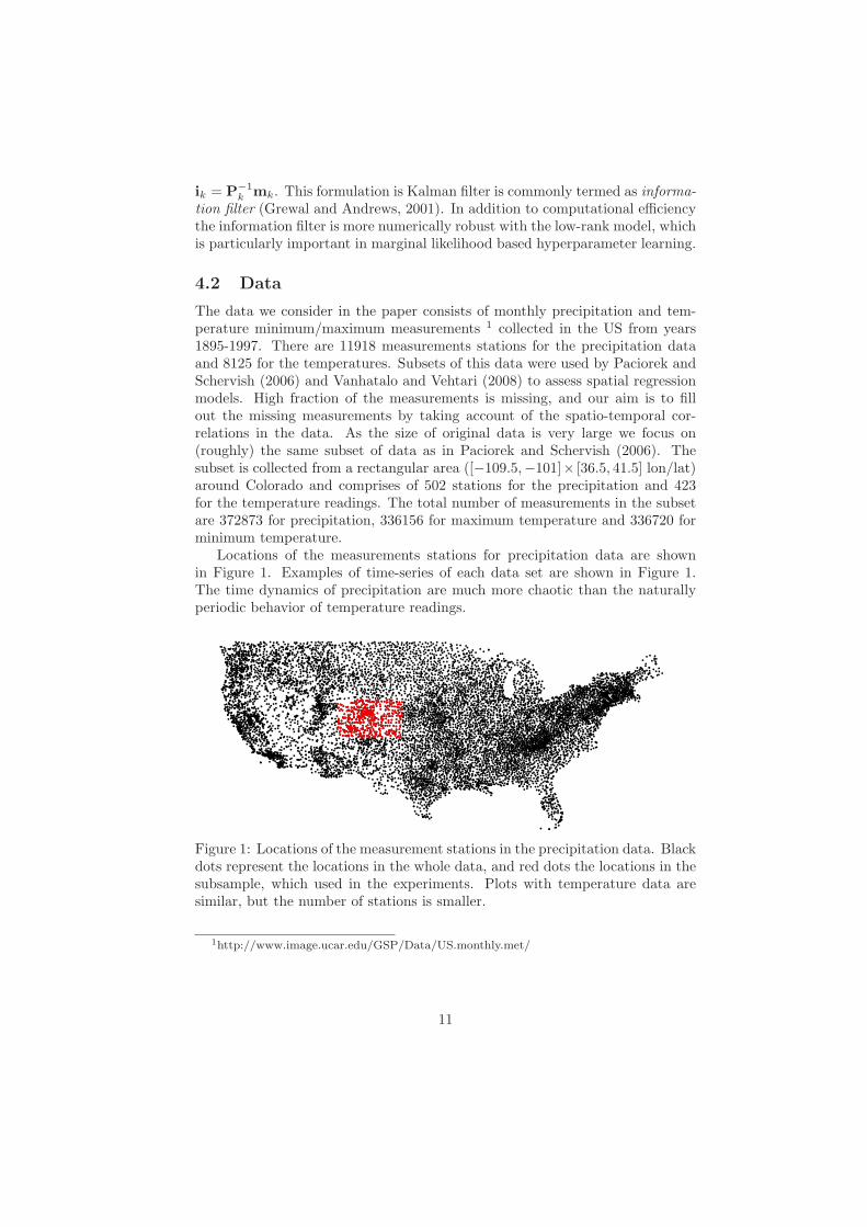
The data we consider in the paper consists of monthly precipitation and tem-perature minimum/maximum measurements 1 collected in the US from years1895-1997. There are 11918 measurements stations for the precipitation dataand 8125 for the temperatures. Subsets of this data were used by Paciorek andSchervish (2006) and Vanhatalo and Vehtari (2008) to assess spatial regressionmodels. High fraction of the measurements is missing, and our aim is to fillout the missing measurements by taking account of the spatio-temporal cor-relations in the data. As the size of original data is very large we focus on(roughly) the same subset of data as in Paciorek and Schervish (2006). Thesubset is collected from a rectangular area ([−109.5,−101]× [36.5, 41.5] lon/lat)around Colorado and comprises of 502 stations for the precipitation and 423for the temperature readings. The total number of measurements in the subsetare 372873 for precipitation, 336156 for maximum temperature and 336720 forminimum temperature.

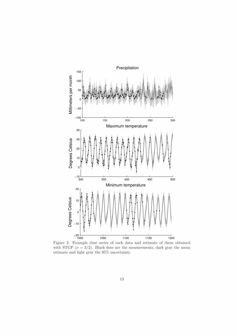
Locations of the measurements stations for precipitation data are shownin Figure 1. Examples of time-series of each data set are shown in Figure 1.The time dynamics of precipitation are much more chaotic than the naturallyperiodic behavior of temperature readings.

Figure 1: Locations of the measurement stations in the precipitation data. Blackdots represent the locations in the whole data, and red dots the locations in thesubsample, which used in the experiments. Plots with temperature data aresimilar, but the number of stations is smaller.

1http://www.image.ucar.edu/GSP/Data/US.monthly.met/

11

References

Cressie, N. and Huang, H.-C. (1999). Classes of nonseparable, spatio-temporal sta-tionary covariance functions. JASA, 94(448):1330–1340.

Grewal, M. S. and Andrews, A. P. (2001). Kalman Filtering, Theory and Practice

Using MATLAB. Wiley Interscience.Hartikainen, J. and Sarkka, S. (2010). Kalman filtering and smoothing solutions to

temporal Gaussian process regression models. In Proceedings of MLSP.Jazwinski, A. (1970). Stochastic Processes and Filtering Theory. Academic Press.Karatzas, I. and Shreve, S. E. (1991). Brownian Motion and Stochastic Calculus.

Springer.Øksendal, B. (2003). Stochastic Differential Equations: An Introduction with Applica-

tions. Springer, 6th edition.Paciorek, C. and Schervish, M. (2006). Spatial modelling using a new class of nonsta-

tionary covariance functions. Environmetrics, 17(5):483–506.Rade, L. and Westergren, B. (2004). Mathematics Handbook. Studentlitteratur, 5th

edition.Rasmussen, C. E. and Williams, C. K. I. (2006). Gaussian Processes for Machine

Learning. MIT Press.Vanhatalo, J. and Vehtari, A. (2008). Modelling local and global phenomena with

sparse Gaussian processes. In Proceedings of UAI.

12

100 150 200 250 300−100

−50

0

50

100

150

PrecipitationM

illim

ete

rs p

er

month

300 350 400 450 500−10

0

10

20

30

40

Maximum temperature

De

gre

es C

els

ius

1000 1050 1100 1150 1200−20

−10

0

10

20

Minimum temperature

De

gre

es C

els

ius

Figure 2: Example time series of each data and estimate of them obtainedwith STGP (ν = 3/2). Black dots are the measurements, dark gray the meanestimate and light gray the 95% uncertainty.

13