www.sciencemag.org/content/344/6179/78/suppl/DC1

Supplementary Material for

The Gravity Field and Interior Structure of Enceladus

L. Iess,* D. J. Stevenson, M. Parisi, D. Hemingway, R. A. Jacobson, J. I. Lunine, F. Nimmo, J. W. Armstrong, S. W. Asmar, M. Ducci, P. Tortora

*Corresponding author. E-mail: luciano.iess@uniroma1.it

Published 4 April 2014, Science 344, 78 (2014)

DOI: 10.1126/science.1250551

This PDF file includes:

Materials and Methods

Supplementary Text

Figs. S1 to S6

Tables S1 to S7

Full Reference List

2

Supplementary Text Contents S1. Enceladus gravity data S2. Data analysis

S2.1. Estimate of Enceladus’ gravity field S2.2. Update of Cassini and Enceladus state vectors S2.3. Residuals S2.4. Gravity disturbances and equipotential heights S2.5. Dynamical model

2.5.1 Gravitational and rotational model 2.5.2 Enceladus’ plumes and other non-gravitational effects

S2.6. Estimate of the ΔVs due to atmospheric drag S3. Model

S3.1. Reference ellipsoid and geoid S3.2. Moment of inertia S3.3. Radau-Darwin S3.4. Effect of a Regional Mass Anomaly S3.5. Isostatic compensation

S1 Enceladus gravity data The Cassini spacecraft performed gravity measurements of Saturn’s icy satellite

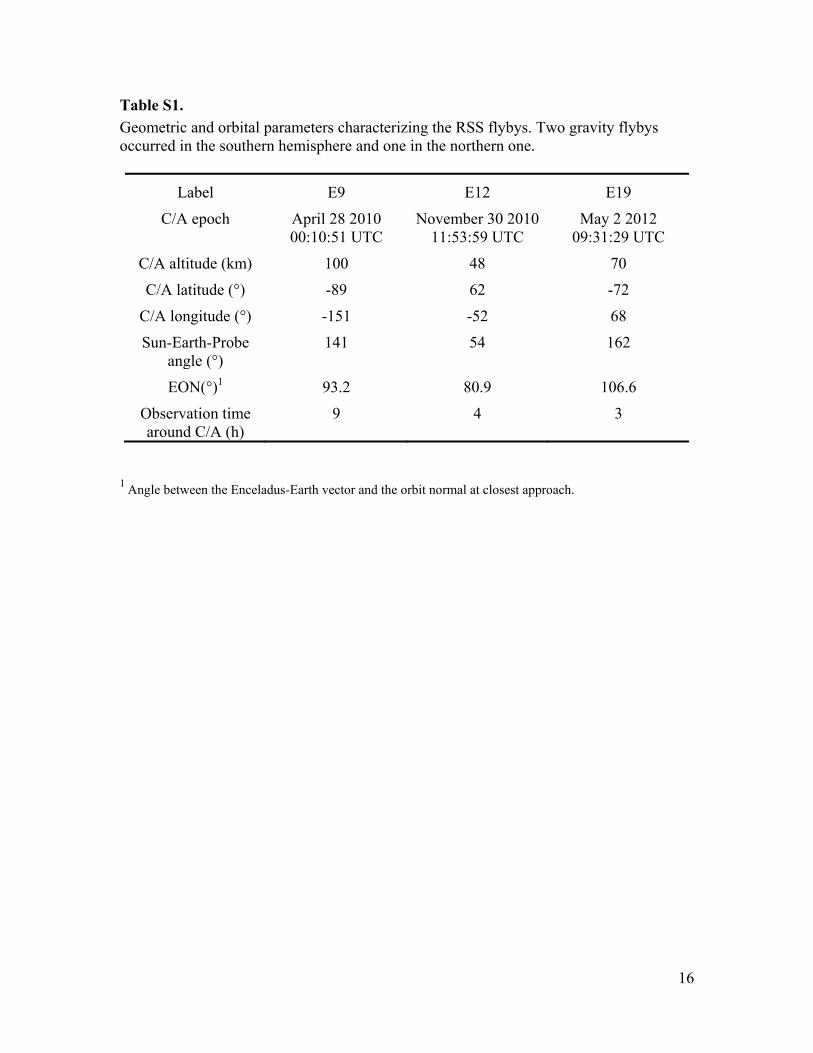
Enceladus between 2010 and 2012. These measurements are crucial to the understanding of the interior structure and evolution of the moon. Due to its size, the determination of the gravity field of this small satellite turned out to be more challenging than that of bigger bodies, also because of the complex dynamics characteristic of the Saturnian system. Cassini encountered Enceladus in three close flybys labeled as E9 (April 2010), E12 (November 2010) and E19 (May 2012), aimed at the determination of the moon’s gravity field by means of Doppler tracking data. These flybys were characterized by low altitudes (within 100 km of the surface) and continuous spacecraft tracking from Earth stations (for at least 3 hours) around closest approach. The south polar region was discovered to be very active and the origin of very interesting physical phenomena. Therefore the gravity investigation was planned so that the spacecraft probed this region twice (17). The key information about the gravity flybys is reported in Table S1.

The spacecraft velocity variation induced by each term of degree l and order m of the gravity field expansion is roughly equal to lma τ , where lma is the corresponding acceleration and τ is the interaction time (in principle different for each harmonics). Neglecting factors of order unity, the perturbations in the spacecraft velocity caused by Enceladus’ gravity (point mass, J2 and J3, respectively) are approximately:

(0) GMVrV

δ ≈ (S1a)

2(2)

2GM RV JrV r

δ ≈

(S1b)

3(3)

3GM RV JrV r

δ ≈

(S1c)

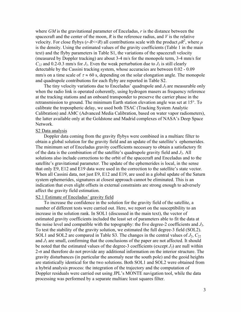
3

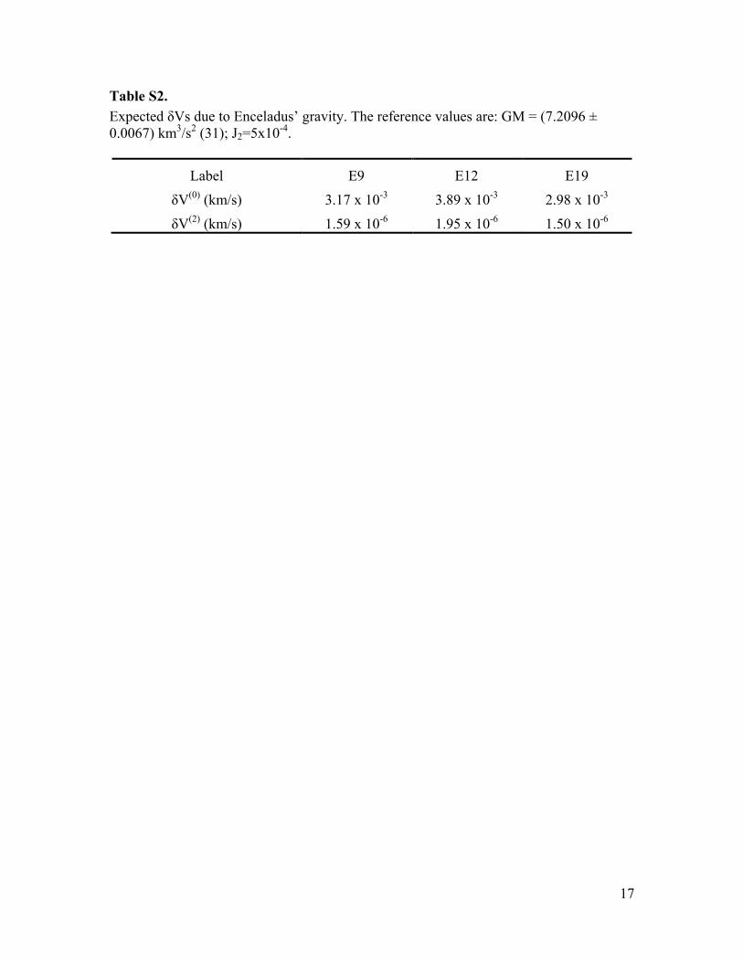
where GM is the gravitational parameter of Enceladus, r is the distance between the spacecraft and the center of the moon, R is the reference radius, and V is the relative velocity. For close flybys (r-R<<R) all contributions scale with the product ρR2, where ρ is the density. Using the estimated values of the gravity coefficients (Table 1 in the main text) and the flyby parameters in Table S1, the variations of the spacecraft velocity (measured by Doppler tracking) are about 3-4 m/s for the monopole term, 3-4 mm/s for C22 and 0.2-0.3 mm/s for J3. Even the weak perturbation due to J3 is still clearly detectable by the Cassini tracking system, whose accuracies are between 0.02 - 0.09 mm/s on a time scale of τ ≈ 60 s, depending on the solar elongation angle. The monopole and quadrupole contributions for each flyby are reported in Table S2.

The tiny velocity variations due to Enceladus’ quadrupole and J3 are measurable only when the radio link is operated coherently, using hydrogen masers as frequency reference at the tracking stations and an onboard transponder to preserve the carrier phase in the retransmission to ground. The minimum Earth station elevation angle was set at 15°. To calibrate the tropospheric delay, we used both TSAC (Tracking System Analytic Calibration) and AMC (Advanced Media Calibration, based on water vapor radiometers), the latter available only at the Goldstone and Madrid complexes of NASA’s Deep Space Network. S2 Data analysis

Doppler data coming from the gravity flybys were combined in a multiarc filter to obtain a global solution for the gravity field and an update of the satellite’s ephemerides. The minimum set of Enceladus gravity coefficients necessary to obtain a satisfactory fit of the data is the combination of the satellite’s quadrupole gravity field and J3. All solutions also include corrections to the orbit of the spacecraft and Enceladus and to the satellite’s gravitational parameter. The update of the ephemerides is local, in the sense that only E9, E12 and E19 data were used in the correction to the satellite’s state vector. When all Cassini data, not just E9, E12 and E19, are used in a global update of the Saturn system ephemerides, signatures at closest approach cannot be eliminated. This is an indication that even slight offsets in external constraints are strong enough to adversely affect the gravity field estimation. S2.1 Estimate of Enceladus’ gravity field

To increase the confidence in the solution for the gravity field of the satellite, a number of different tests were carried out. Here, we report on the susceptibility to an increase in the solution rank. In SOL1 (discussed in the main text), the vector of estimated gravity coefficients included the least set of parameters able to fit the data at the noise level and compatible with the topography: the five degree-2 coefficients and J3. To test the stability of the gravity solution, we estimated the full degree-3 field (SOL2). SOL1 and SOL2 are compared in Table S3. The changes in the central values of J2, C22 and J3 are small, confirming that the conclusions of the paper are not affected. It should be noted that the estimated values of the degree-3 coefficients (except J3) are null within 2-σ and therefore do not provide any additional information on the interior structure. The gravity disturbances (in particular the anomaly near the south pole) and the geoid heights are statistically identical for the two solutions. Both SOL1 and SOL2 were obtained from a hybrid analysis process: the integration of the trajectory and the computation of Doppler residuals were carried out using JPL’s MONTE navigation tool, while the data processing was performed by a separate multiarc least squares filter.

4

S.2.2 Update of Cassini and Enceladus state vectors The estimation of Enceladus’ mass and gravity coefficients required an update of the

spacecraft and the satellite initial states, at a reference epoch prior to the first gravity flyby. This process yielded new values for Enceladus’ gravitational parameter and reference state. Since the mass and the trajectory of the system barycenter must be kept unchanged during the iterative process, this resulted in a small adjustment of all major Saturnian satellite ephemerides. Corrections to the state of the spacecraft and Enceladus were made with respect to the nominal Cassini trajectory, provided by the navigation team, and JPL’s satellite ephemerides (sat337), respectively. JPL’s planetary ephemerides de421were used for the orbit of Saturn system barycenter. S2.3 Residuals

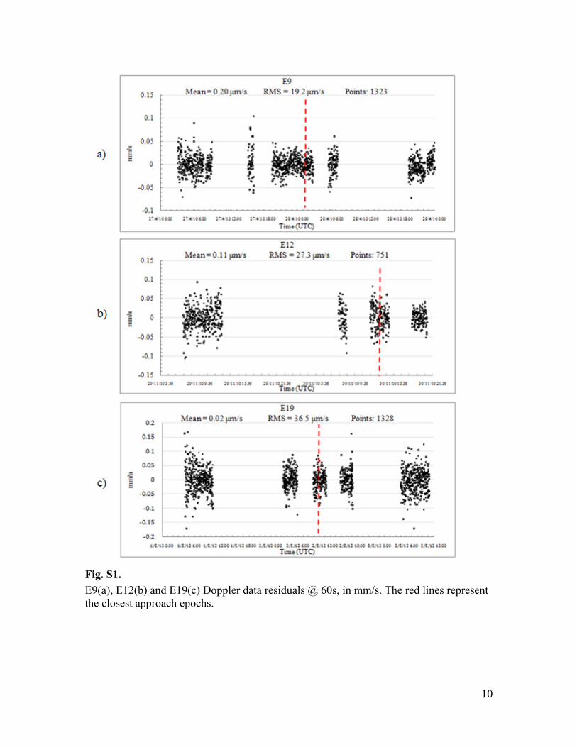
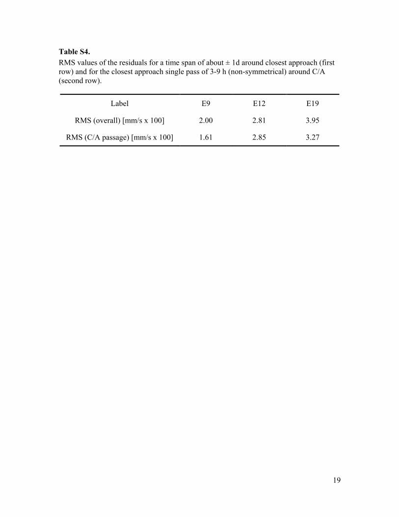
In this section, we discuss the Doppler residuals relative to the three gravity flybys, achieved as outcomes of the data processing. The count time for Doppler tracking data was set to 60 seconds. For this analysis only two-way and three-way Doppler data were used (F2 and F3), from X/X and X/Ka links. The time span of our data analysis was about 2 days centered at the closest approach, for each flyby. The plots in Figure S1 are free from signatures, zero-mean and nearly Gauss-distributed around the mean values. The RMS value of the residuals is reported in Table S4. S.2.4 Gravity disturbances and equipotential heights

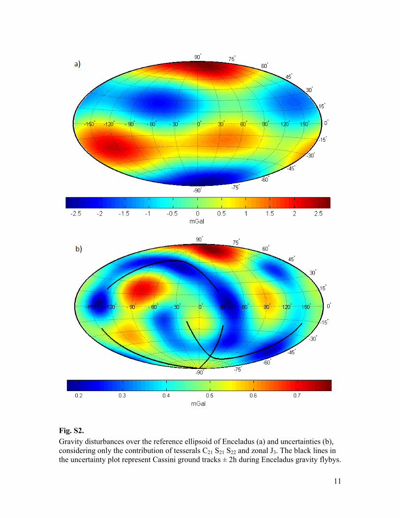
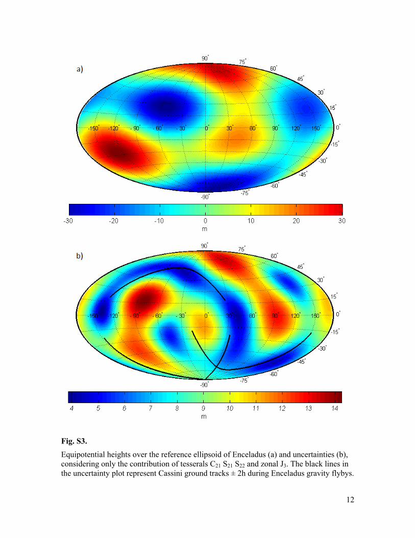
Using the coefficients estimated in SOL1, we produced a set of plots (Figures S2 and S3) showing the gravity disturbances and the equipotential heights over Enceladus’ reference ellipsoid, respectively, due to the effect of C21, S21, S22 and J3. The satellite presents a negative gravity anomaly at the south pole, of about 2.5 mGal. This anomaly arises in the equipotential height plot as a depression of about 30 m over the ellipsoid. The uncertainties over the gravity disturbances Δg (Figure S2b) are computed as:

2T

gg gCx x

σ∆

∂∆ ∂∆ = ∂ ∂ (S2)

where 2,0 ,... N Nx GM J J − = is the vector of the gravity parameters and C is the covariance matrix associated to the estimate of x. Similarly, the uncertainty on the geoid heights can be expressed as:

2T

rr rC

x xσ∆

∂∆ ∂∆ = ∂ ∂ (S3)

although in Figure S2 and S3 we did not include the contributions from J2 and C22 in equations S2 and S3 and referred the disturbances and geoid heights to the reference ellipsoid. S.2.5 Dynamical model

In order to obtain a satisfactory fit of Enceladus’ gravity data, it is of primary importance to correctly account for the effects of gravitational and non-gravitational forces acting on the spacecraft. In the following sections we discuss the details of relevant choices made in the process of building the most realistic possible dynamical environment surrounding the Cassini spacecraft during the gravity flybys of Enceladus. S.2.5.1 Gravitational and rotational model

In the dynamical model used for the analysis of Enceladus gravity data, we took into account the point mass accelerations exerted by all planets and saturnian satellites

5

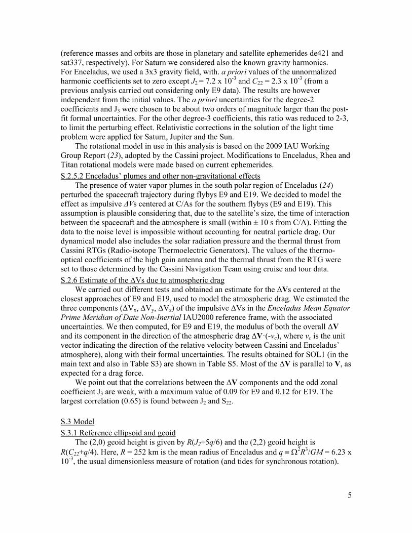
(reference masses and orbits are those in planetary and satellite ephemerides de421 and sat337, respectively). For Saturn we considered also the known gravity harmonics. For Enceladus, we used a 3x3 gravity field, with. a priori values of the unnormalized harmonic coefficients set to zero except J2 = 7.2 x 10-3 and C22 = 2.3 x 10-3 (from a previous analysis carried out considering only E9 data). The results are however independent from the initial values. The a priori uncertainties for the degree-2 coefficients and J3 were chosen to be about two orders of magnitude larger than the post-fit formal uncertainties. For the other degree-3 coefficients, this ratio was reduced to 2-3, to limit the perturbing effect. Relativistic corrections in the solution of the light time problem were applied for Saturn, Jupiter and the Sun.

The rotational model in use in this analysis is based on the 2009 IAU Working Group Report (23), adopted by the Cassini project. Modifications to Enceladus, Rhea and Titan rotational models were made based on current ephemerides. S.2.5.2 Enceladus’ plumes and other non-gravitational effects

The presence of water vapor plumes in the south polar region of Enceladus (24) perturbed the spacecraft trajectory during flybys E9 and E19. We decided to model the effect as impulsive ΔVs centered at C/As for the southern flybys (E9 and E19). This assumption is plausible considering that, due to the satellite’s size, the time of interaction between the spacecraft and the atmosphere is small (within ± 10 s from C/A). Fitting the data to the noise level is impossible without accounting for neutral particle drag. Our dynamical model also includes the solar radiation pressure and the thermal thrust from Cassini RTGs (Radio-isotope Thermoelectric Generators). The values of the thermo-optical coefficients of the high gain antenna and the thermal thrust from the RTG were set to those determined by the Cassini Navigation Team using cruise and tour data. S.2.6 Estimate of the ΔVs due to atmospheric drag

We carried out different tests and obtained an estimate for the ΔVs centered at the closest approaches of E9 and E19, used to model the atmospheric drag. We estimated the three components (ΔVx, ΔVy, ΔVz) of the impulsive ΔVs in the Enceladus Mean Equator Prime Meridian of Date Non-Inertial IAU2000 reference frame, with the associated uncertainties. We then computed, for E9 and E19, the modulus of both the overall ΔV and its component in the direction of the atmospheric drag ΔV·(-vc), where vc is the unit vector indicating the direction of the relative velocity between Cassini and Enceladus’ atmosphere), along with their formal uncertainties. The results obtained for SOL1 (in the main text and also in Table S3) are shown in Table S5. Most of the ΔV is parallel to V, as expected for a drag force.

We point out that the correlations between the ΔV components and the odd zonal coefficient J3 are weak, with a maximum value of 0.09 for E9 and 0.12 for E19. The largest correlation (0.65) is found between J2 and S22.

S.3 Model S.3.1 Reference ellipsoid and geoid

The (2,0) geoid height is given by R(J2+5q/6) and the (2,2) geoid height is R(C22+q/4). Here, R = 252 km is the mean radius of Enceladus and q ≡ Ω2R3/GM = 6.23 x 10-3, the usual dimensionless measure of rotation (and tides for synchronous rotation).

6

The reference ellipsoid is the equipotential surface for the (2,0) and (2,2) gravity harmonics, and centrifugal and tidal potential. The uncertainties in the short (polar) and long axis of the reference ellipsoid are respectively 9 and 16 m. S.3.2 Moment of inertia

We express the mean moment of inertia I as αMR2. Consider a body consisting of two layers, a core of radius xR and density Aρ0 and a mantle of density ρ0. The mean satellite density is ρ .

( ) 3

0

1 1r A xρρ

≡ = − + (S4)

( ) 52 1 15

r A xα ≡ − + (S5)

whence:

5 12

1

rx

r

α − =

− (S6)

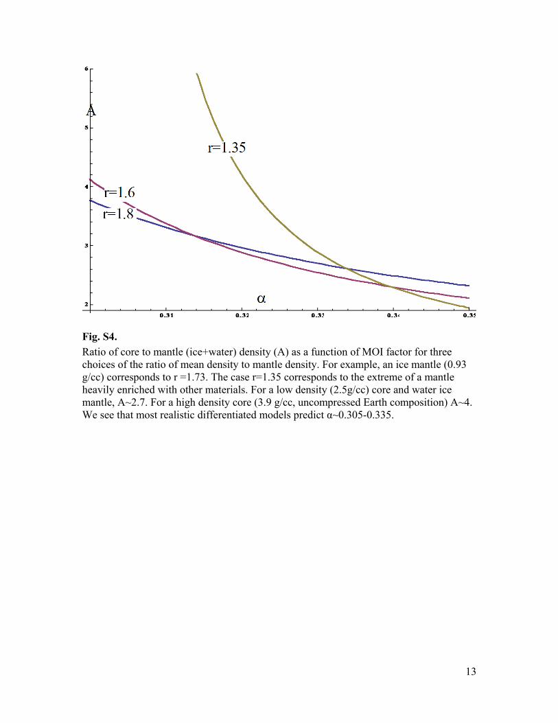
and A can be expressed explicitly in terms of α and r alone, see Figure S4. This formulation can only be used for small, differentiated satellites, since it depends on the ice layer having uniform density. There are no comparable satellites to Enceladus for which a useful comparison can be made. Rhea is the only other small satellite where the quadrupole field is available and several attempts have been made to interpret the data, with disagreement about the extent of differentiation and hydrostaticity (33-36).

A three-layer model could also be constructed in order to distinguish between the liquid and solid portions of the mantle. Assuming that ice and water densities differ by only ~10%, however, the effect on moment of inertia is negligible and therefore we prefer the two layer model for its simplicity. S.3.3 Radau-Darwin

The prediction of Radau-Darwin, linearized near the region of interest (0.32 < α < 0.35), is adequately approximated by:

( )( )

6 42,h

6 422,h

10 J = 5000+3.850x10 0.33410 = 1500+1.155x10 0.334C

αα−−

(S7)

for the hydrostatic contributions, exactly satisfying the 10/3 ratio. We can write: 2 2,h 2,nhJ J J= + (S8)

22 22,h 22,nhC C C= + (S9) for the hydrostatic and non-hydrostatic contributions, respectively. S.3.4. Effect of a Regional Mass Anomaly

The standard expansion of 1 'r r− in terms of Legendre polynomials implies that a

point mass at the South pole would yield a gravity field with contributions of the form J2n = -J2n+1 where n is a positive integer and the magnitude of the anomaly is proportional to the point mass δm. If instead that mass anomaly is spread uniformly over a latitude range as a cap centered on the south pole then the prediction is:

7

( ) ( )3 2 42 3 2 3

1 1

( ) / ( ) / 2 / 2 / 1/ 8 3 / 4 5 / 8x x

J J P x dx P x dx x x x x− −

= = − + − +∫ ∫ (S10)

where x = cosθ and θ is colatitude (x = -1 at the south pole). S.3.5 Isostatic compensation

Generalizing from equations (S8) and (S9), the measured non-normalized spherical harmonic gravity coefficients Glm may be separated into their hydrostatic (h) and non-hydrostatic (nh) components:

h nhlm lm lmG G G= + (S11)

Similarly the topographic coefficients derived from limb profiles (12) may be likewise separated:

h nhlm lm lmH H H= + (S12)

Taking the present-day rotation rate, the Darwin-Radau approximation (25) may then be used to calculate , , and given an assumed dimensionless moment of inertia α = I/MR2. The (3,0) terms have no hydrostatic component.

We then define the admittance Zlm as the ratio of the non-hydrostatic gravity to non-hydrostatic topography (26):

/nh nhlm lm lmZ G H= (S13)

The admittance gives an indication of the degree to which the topography is compensated and the depth at which compensation occurs, and can be estimated separately from the gravity-to-topography ratios for the (2,0), (2,2) and (3,0) terms (i.e., giving Z20, Z22, and Z30).

To determine the implied degree and depth of compensation, we note that the expected degree-l, order-m admittance is given by (26):

( )

3 1 12 1

lc

lmdZ C

l R Rρ

ρ = − − +

(S14)

where C is the degree of compensation (C=0 when the topography is uncompensated and C=1 when the topography is fully compensated, assuming surface loading), d is the depth of compensation, cρ is the crustal (ice shell) density, ρ is the mean density of Enceladus, and R is the mean radius of Enceladus. If, rather than surface loading, the topography arises due to loading from the bottom of the ice shell, we have:

( )

3 11 12 1

lc

lmdZ

l R C Rρ

ρ = − − +

(S14b)

Equation S14 can also be rewritten as:

( )

32 1

clm lmZ f

l Rρ

ρ=

+ (S15)

where flm captures both the degree of compensation and the compensation depth. If we assume complete compensation, then ( )1 1 l

lmf d R= − − (see Table 2 in the main text). Assuming isotropic admittance (expected from S14 as long as compensation is isotropic), the degree-2 admittances estimated separately from the (2,0) and (2,2) terms should agree

8

when the correct moment of inertia (α) is assumed. In this situation, f20 and f22 should likewise agree. Figure S6 plots Z20 and Z22 as a function of α and shows that there is a range of α values for which the two admittance estimates agree.

The (3,0) terms provide an independent check on the assumption of isotropic admittance. The ratio Z20/Z30 should be approximately 0.991 assuming a fully isostatic ice shell of mean thickness 30 km (eq. S14) and the properties listed in Table S6. Figure S6 shows that the measured value of Z30, when corrected by this factor, plots in the middle of the region in which Z20 and Z22 agree. This result provides an a posteriori check that the assumption of isotropic admittance is appropriate.

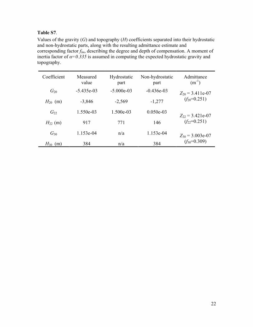
Agreement between the three estimates occurs at the 1-σ level for normalized moments of inertia (α =I/MR2) in the range 0.333–0.338 and admittances in the range 2.4–3.6 × 10-7 m-1 (Figure S6). The equivalent range of f20=f22 is 0.18-0.26, taking ρc=0.92 g/cc and assuming complete compensation. Agreement at the 2-σ level occurs in the range α = 0.330–0.340 and Z2 = 1.8–4.2 × 10-7 m-1 (f20=f22=0.13-0.31). Table S7 lists the gravity and topography coefficients separated into their hydrostatic and non-hydrostatic parts, along with the resulting admittances.

The regions of agreement were obtained by performing a Monte Carlo analysis in which each admittance value is calculated 100,000 times with the gravity and topography coefficients normally distributed according to their formal uncertainties. The regions in which there is overlap between the resulting 1-σ ranges of the three separate admittance estimates (based on the (2,0), (2,2), and (3,0) terms) is considered to be the region of agreement at the 1-σ level. The same procedure was carried out to determine the region of agreement at the 2-σ level.

The above analysis is model-independent, in that it makes no assumption about the location of the gravity anomalies (though it does assume isotropic admittance). However, if the only source of non-hydrostatic gravity were the surface topography, the non-hydrostatic gravity would be much larger than that observed (and the admittance would be ~14x10-7 m-1). This result strongly suggests that some kind of compensation, either regional or global, is taking place.

One end-member compensation model is to assume that compensation occurs at the base of an ice shell floating on a global ocean (27). In this case, adopting the parameters given in Table S6, we estimate the compensation depth (i.e., ice shell thickness) required to match the calculated admittance to be roughly 20–40 km (see Figure S6 and eq. S14).

Elastic thicknesses greater than ~0.5 km greatly reduce compensation and therefore lead to admittances that are too great (in the case of top-loading) or too small (in the case of bottom-loading) to agree with the values estimated here (26, 28). The top-loading calculation is carried out using equation S14 where the compensation factor, C=C(∆ρ), is computed according to equations S19 and S22 from ref. 26; the bottom-loading calculation instead uses equation S14b, with C=C(ρc), again computed according to equations S19 and S22 from ref. 26 (see Table S6 for the parameters used in these calculations). The small implied elastic thickness is in agreement with a local estimate of 0.3 km (13) based on flexural analysis and consistent with high heat fluxes inferred from relaxation studies (14).

If a global ocean is present, it will have observational consequences. In particular, the amplitude of longitudinal librations will be increased beyond those predicted for a solid Enceladus (21), with possibly important consequences for plume eruptive behavior;

9

the same will be true of the obliquity, although this is predicted to be very small (29). Non-synchronous rotation, which has been suggested on the basis of geological mapping (30), is possible, and true polar wander (31) is more likely.

It has been suggested that Enceladus may experience a 1:3 or 1:4 spin-orbit resonance, resulting in large amplitude librations (17, 22). The ratio of the librational frequency to the orbital frequency is given by (22):

1/222

2

32/C

C MRε =

(S16)

For the SOL1 value of C22 and C/MR2=0.335, we obtain ε=0.236, with a 2σ uncertainty of 0.003. This value of ε is less than that required for a 1:4 spin orbit resonance to occur.

Lastly, the global ocean makes predictions for the size of G40. Again assuming full compensation and a shell thickness of ~30 km, the ratio Z40/Z30 should be 0.978 and so based on the measured Z30 we obtain Z40=2.94 x10-7 m-1. Together with the known value of H40 (=-177 m), the predicted value of G40 is -5.22x10-5, or just less than half the magnitude of G30.

10

Fig. S1. E9(a), E12(b) and E19(c) Doppler data residuals @ 60s, in mm/s. The red lines represent the closest approach epochs.

11

Fig. S2. Gravity disturbances over the reference ellipsoid of Enceladus (a) and uncertainties (b), considering only the contribution of tesserals C21 S21 S22 and zonal J3. The black lines in the uncertainty plot represent Cassini ground tracks ± 2h during Enceladus gravity flybys.

12

Fig. S3. Equipotential heights over the reference ellipsoid of Enceladus (a) and uncertainties (b), considering only the contribution of tesserals C21 S21 S22 and zonal J3. The black lines in the uncertainty plot represent Cassini ground tracks ± 2h during Enceladus gravity flybys.

13

Fig. S4. Ratio of core to mantle (ice+water) density (A) as a function of MOI factor for three choices of the ratio of mean density to mantle density. For example, an ice mantle (0.93 g/cc) corresponds to r =1.73. The case r=1.35 corresponds to the extreme of a mantle heavily enriched with other materials. For a low density (2.5g/cc) core and water ice mantle, A~2.7. For a high density core (3.9 g/cc, uncompressed Earth composition) A~4. We see that most realistic differentiated models predict α~0.305-0.335.

14

Fig. S5. Thickness (D) of the mantle (water+ice) as a function of MOI factor for different choices of r, the ratio of mean density to mantle density. Mantle thicknesses of 60-100km are typical except when the mantle is much more dense than water ice.

15

Fig. S6. Region of 1-σ agreement (dark blue) and 2-σ agreement (pale blue) between the admittances estimated separately from the (2,0) (blue line), (2,2) (red line), and (3,0) (green line) terms. The (3,0) term has been multiplied by 0.991 to obtain the equivalent degree-2 value (see text). The solid line at ~14 × 10-7 /m represents the admittance expected for uncompensated (rigidly supported) topography. The dashed horizontal lines near 2 and 4 × 10-7 /m represent the admittances expected for fully compensated topography with compensation depths (ice shell thicknesses) of 20 and 40 km, respectively.

16

Table S1. Geometric and orbital parameters characterizing the RSS flybys. Two gravity flybys occurred in the southern hemisphere and one in the northern one.

Label E9 E12 E19

C/A epoch April 28 2010 00:10:51 UTC

November 30 2010 11:53:59 UTC

May 2 2012 09:31:29 UTC

C/A altitude (km) 100 48 70

C/A latitude (°) -89 62 -72

C/A longitude (°) -151 -52 68

Sun-Earth-Probe angle (°)

141 54 162

EON(°)1 93.2 80.9 106.6

Observation time around C/A (h)

9 4 3

1 Angle between the Enceladus-Earth vector and the orbit normal at closest approach.

17

Table S2. Expected δVs due to Enceladus’ gravity. The reference values are: GM = (7.2096 ± 0.0067) km3/s2 (31); J2=5x10-4.

Label E9 E12 E19

δV(0) (km/s) 3.17 x 10-3 3.89 x 10-3 2.98 x 10-3

δV(2) (km/s) 1.59 x 10-6 1.95 x 10-6 1.50 x 10-6

18

Table S3. Estimated gravity field of Enceladus (SOL1 And SOL2). ΔV(E9) and ΔV(E19) are the closest approach ΔVs used to model the effect of atmospheric drag (see Section S2.5.2 and Table S5).

Coefficient RSS (SOL1) RSS (SOL2) [km3/s2] [km3/s2]

GM 7.210443 ± 0.000030 7.210419 ± 0.000035 [value ± 1σ (x106)] [value ± 1σ (x106)]

J2 5435.2 ± 34.9 5442.9 ± 69.3 C21 9.2 ± 11.6 -59.2 ± 43.6 S21 39.8 ± 22.4 20.2 ± 67.7 C22 1549.8 ± 15.6 1613.5 ± 51.8 S22 22.6 ± 7.4 14.9 ± 13.5 J3 -115.3 ± 22.9 -85.9 ± 69.8

C31 / -40.3 ± 48.2 S31 / -97.4 ± 40.5 C32 / 33.3 ± 19.4 S32 / 8.1 ± 14.6 C32 / -1.5 ± 8.9 S32 / -15.0 ± 9.0

[mm/s] [mm/s] ΔV (E9) 0.247 ± 0.053 0.243 ± 0.054 ΔV (E19) 0.256 ± 0.049 0.261 ± 0.051

19

Table S4. RMS values of the residuals for a time span of about ± 1d around closest approach (first row) and for the closest approach single pass of 3-9 h (non-symmetrical) around C/A (second row).

Label E9 E12 E19

RMS (overall) [mm/s x 100] 2.00 2.81 3.95

RMS (C/A passage) [mm/s x 100] 1.61 2.85 3.27

20

Table S5. Estimated values for the ΔVs at E9 and E19 closest approaches. The component of the velocity variation along the drag direction is ΔV// = ΔV · (-vc) and is, in both cases, more the 90% of the total ΔV.

Flyby Component Central value

[mm/s]

Formal uncertainty

[mm/s]

Relative uncertainty

[%]

ΔV// / ΔV [%]

E9

ΔVx 0.1382 0.0273

ΔVy 0.2042 0.0419

ΔVz 0.0012 0.0493

ΔV 0.2466 0.0531 21.55 ΔV// = ΔV · (-vc) 0.2280 0.0457 20.04 92.46

E19

ΔVx -0.1766 0.0276

ΔVy 0.1817 0.0465

ΔVz -0.0384 0.0492

ΔV 0.2563 0.0490 19.49

ΔV// = ΔV · (-vc) 0.2333 0.0386 16.56 91.03

21

Table S6. Parameter values adopted in computing model admittances.

Parameter Symbol Value

Young’s modulus for ice E 9 GPa

Crustal (ice shell) density ρc 920 kg/m

3

Mantle (ocean) density ρm 1000 kg/m

3

Enceladus' bulk density 1609 kg/m3

Enceladus' radius R 252.1 km

Enceladus' surface gravity g 0.114 m/s2

22

Table S7. Values of the gravity (G) and topography (H) coefficients separated into their hydrostatic and non-hydrostatic parts, along with the resulting admittance estimate and corresponding factor flm, describing the degree and depth of compensation. A moment of inertia factor of α=0.335 is assumed in computing the expected hydrostatic gravity and topography.

Coefficient Measured value

Hydrostatic part

Non-hydrostatic part

Admittance (m-1)

G20 -5.435e-03 -5.000e-03 -0.436e-03 Z20 = 3.411e-07 (f20=0.251) H20 (m) -3,846 -2,569 -1,277

G22 1.550e-03 1.500e-03 0.050e-03 Z22 = 3.421e-07

(f22=0.251) H22 (m) 917 771 146

G30 1.153e-04 n/a 1.153e-04 Z30 = 3.003e-07 (f30=0.309) H30 (m) 384 n/a 384

References and Notes 1. J. N. Spitale, C. C. Porco, Association of the jets of Enceladus with the warmest regions on its

south-polar fractures. Nature 449, 695–697 (2007). doi:10.1038/nature06217 Medline

2. F. Postberg, J. Schmidt, J. Hillier, S. Kempf, R. Srama, A salt-water reservoir as the source of a compositionally stratified plume on Enceladus. Nature 474, 620–622 (2011). doi:10.1038/nature10175 Medline

3. J. R. Spencer, J. C. Pearl, M. Segura, F. M. Flasar, A. Mamoutkine, P. Romani, B. J. Buratti, A. R. Hendrix, L. J. Spilker, R. M. Lopes, Cassini encounters Enceladus: Background and the discovery of a south polar hot spot. Science 311, 1401–1405 (2006). doi:10.1126/science.1121661

4. M. M. Hedman, C. M. Gosmeyer, P. D. Nicholson, C. Sotin, R. H. Brown, R. N. Clark, K. H. Baines, B. J. Buratti, M. R. Showalter, An observed correlation between plume activity and tidal stresses on Enceladus. Nature 500, 182–184 (2013). doi:10.1038/nature12371 Medline

5. C. J. A. Howett, J. R. Spencer, J. Pearl, M. Segura, High heat flow from Enceladus’ south polar region measured using 10–600 cm−1 Cassini/CIRS data. J. Geophys. Res. 116, (E3), E03003 (2011). doi:10.1029/2010JE003718

6. J. Meyer, J. Wisdom, Tidal heating in Enceladus. Icarus 188, 535–539 (2007). doi:10.1016/j.icarus.2007.03.001

7. G. W. Ojakangas, D. J. Stevenson, Episodic volcanism of tidally heated satellites with application to Io. Icarus 66, 341–358 (1986). doi:10.1016/0019-1035(86)90163-6

8. K. Zhang, F. Nimmo, Recent orbital evolution and the internal structures of Enceladus and Dione. Icarus 204, 597–609 (2009). doi:10.1016/j.icarus.2009.07.007

9. Materials and methods are available as supplementary materials on Science Online.

10. L. Iess, N. J. Rappaport, R. A. Jacobson, P. Racioppa, D. J. Stevenson, P. Tortora, J. W. Armstrong, S. W. Asmar, Gravity field, shape, and moment of inertia of Titan. Science 327, 1367–1369 (2010). doi:10.1126/science.1182583

11. L. Iess, R. A. Jacobson, M. Ducci, D. J. Stevenson, J. I. Lunine, J. W. Armstrong, S. W. Asmar, P. Racioppa, N. J. Rappaport, P. Tortora, The tides of Titan. Science 337, 457–459 (2012). doi:10.1126/science.1219631

12. F. Nimmo, B. G. Bills, P. C. Thomas, Geophysical implications of the long-wavelength topography of the Saturnian satellites. J. Geophys. Res. 116, E11001 (2011). doi:10.1029/2011JE003835

13. B. Giese, R. Wagner, H. Hussmann, G. Neukum, J. Perry, P. Helfenstein, P. C. Thomas, Enceladus: An estimate of heat flux and lithospheric thickness from flexurally supported topography. Geophys. Res. Lett. 35, L24204 (2008). doi:10.1029/2008GL036149

14. M. T. Bland, K. N. Singer, W. B. McKinnon, P. M. Schenk, Enceladus’ extreme heat flux as revealed by its relaxed craters. Geophys. Res. Lett. 39, L17204 (2012). doi:10.1029/2012GL052736

15. G. Schubert, J. D. Anderson, B. J. Travis, J. Palguta, Enceladus: Present internal structure and differentiation by early and long-term radiogenic heating. Icarus 188, 345–355 (2007). doi:10.1016/j.icarus.2006.12.012

16. S. Zhong et al., J. Geophys. Res. 39, L15201 (2012).

17. C. C. Porco, P. Helfenstein, P. C. Thomas, A. P. Ingersoll, J. Wisdom, R. West, G. Neukum, T. Denk, R. Wagner, T. Roatsch, S. Kieffer, E. Turtle, A. McEwen, T. V. Johnson, J. Rathbun, J. Veverka, D. Wilson, J. Perry, J. Spitale, A. Brahic, J. A. Burns, A. D. Delgenio, L. Dones, C. D. Murray, S. Squyres, Cassini observes the active south pole of Enceladus. Science 311, 1393–1401 (2006). doi:10.1126/science.1123013

18. W. B. McKinnon, J. Geophys. Res. 118, 1775 (2013). doi:10.1002/jgrc.20072

19. G. Tobie, O. Cadek, C. Sotin, Solid tidal friction above a liquid water reservoir as the origin of the south pole hotspot on Enceladus. Icarus 196, 642–652 (2008). doi:10.1016/j.icarus.2008.03.008

20. J. H. Roberts, F. Nimmo, Tidal heating and the long-term stability of a subsurface ocean on Enceladus. Icarus 194, 675–689 (2008). doi:10.1016/j.icarus.2007.11.010

21. N. Rambaux, J. C. Castillo-Rogez, J. G. Williams, Ö. Karatekin, Librational response of Enceladus. Geophys. Res. Lett. 37, L04202 (2010). doi:10.1029/2009GL041465

22. J. Wisdom, Spin-orbit secondary resonance dynamics of Enceladus. Astron. J. 128, 484–491 (2004). doi:10.1086/421360

23. B. A. Archinal, M. F. A’Hearn, E. Bowell, A. Conrad, G. J. Consolmagno, R. Courtin, T. Fukushima, D. Hestroffer, J. L. Hilton, G. A. Krasinsky, G. Neumann, J. Oberst, P. K. Seidelmann, P. Stooke, D. J. Tholen, P. C. Thomas, I. P. Williams, Report of the IAU Working Group on cartographic coordinates and rotational elements: 2009. Celestial Mech. Dyn. Astron. 109, 101–135 (2011). doi:10.1007/s10569-010-9320-4

24. J. H. Waite, Jr., M. R. Combi, W. H. Ip, T. E. Cravens, R. L. McNutt, Jr., W. Kasprzak, R. Yelle, J. Luhmann, H. Niemann, D. Gell, B. Magee, G. Fletcher, J. Lunine, W. L. Tseng, Cassini ion and neutral mass spectrometer: Enceladus plume composition and structure. Science 311, 1419–1422 (2006). doi:10.1126/science.1121290

25. C. D. Murray, S. F. Dermott, Solar System Dynamics (Cambridge Univ. Press, Cambridge, 2000), pp. XXX–XXX.

26. D. Hemingway, F. Nimmo, H. Zebker, L. Iess, A rigid and weathered ice shell on Titan. Nature 500, 550–552 (2013). doi:10.1038/nature12400 Medline

27. G. C. Collins, J. C. Goodman, Enceladus’ south polar sea. Icarus 189, 72–82 (2007). doi:10.1016/j.icarus.2007.01.010

28. D. L. Turcotte, R. J. Willemann, W. F. Haxby, J. Norberry, Role of membrane stresses in the support of planetary topography. J. Geophys. Res. 86, 3951 (1981). doi:10.1029/JB086iB05p03951

29. E. M. A. Chen, F. Nimmo, Obliquity tides do not significantly heat Enceladus. Icarus 214, 779–781 (2011). doi:10.1016/j.icarus.2011.06.007

30. D. A. Patthoff, S. A. Kattenhorn, A fracture history on Enceladus provides evidence for a global ocean. Geophys. Res. Lett. 38, L18201 (2011). doi:10.1029/2011GL048387

31. F. Nimmo, R. T. Pappalardo, Diapir-induced reorientation of Saturn’s moon Enceladus. Nature 441, 614–616 (2006). doi:10.1038/nature04821 Medline

32. R. A. Jacobson, P. G. Antreasian, J. J. Bordi, K. E. Criddle, R. Ionasescu, J. B. Jones, R. A. Mackenzie, M. C. Meek, D. Parcher, F. J. Pelletier, W. M. Owen, Jr., D. C. Roth, I. M. Roundhill, J. R. Stauch, The gravity field of the Saturnian system from satellite observations and spacecraft tracking data. Astron. J. 132, 2520–2526 (2006). doi:10.1086/508812

33. J. D. Anderson, G. Schubert, Geophys. Res. Lett. 34, L02202 (2007).

34. L. Iess, N. Rappaport, P. Tortora, J. Lunine, J. Armstrong, S. Asmar, L. Somenzi, F. Zingoni, Gravity field and interior of Rhea from Cassini data analysis. Icarus 190, 585–593 (2007). doi:10.1016/j.icarus.2007.03.027

35. R. A. MacKenzie, L. Iess, P. Tortora, N. J. Rappaport, A non-hydrostatic Rhea. Geophys. Res. Lett. 35, L05204 (2008). doi:10.1029/2007GL032898

36. J. D. Anderson, G. Schubert, Rhea’s gravitational field and interior structure inferred from archival data files of the 2005 Cassini flyby. Phys. Earth Planet. Inter. 178, 176–182 (2010). doi:10.1016/j.pepi.2009.09.003