Supplementary Information Integrative Genomics ViewerAny numeric data IGV, WIG, TDF Sample metatadata Tab-delimited sample info file Table 4. IGV file formats. Sample Information File

1

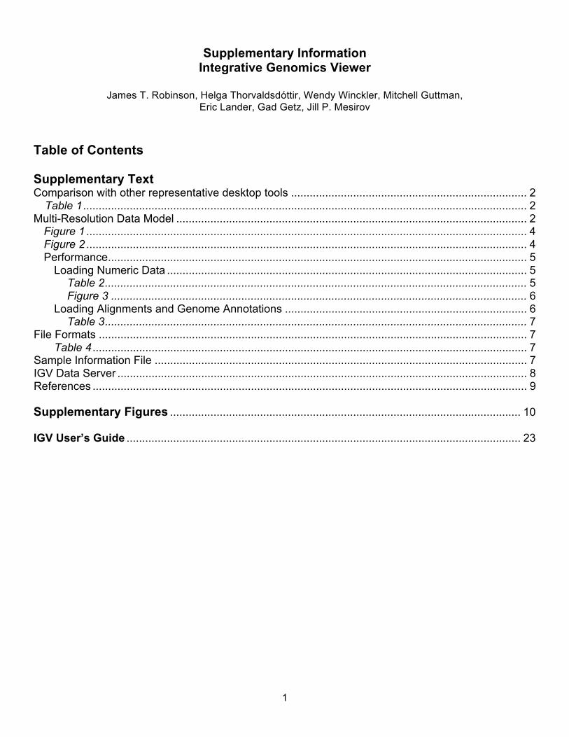
Supplementary Information Integrative Genomics Viewer

James T. Robinson, Helga Thorvaldsdóttir, Wendy Winckler, Mitchell Guttman,

Eric Lander, Gad Getz, Jill P. Mesirov

Table of Contents Supplementary Text Comparison with other representative desktop tools ............................................................................ 2 Table 1............................................................................................................................................... 2Multi-Resolution Data Model ................................................................................................................. 2

Figure 1 .............................................................................................................................................. 4 Figure 2 .............................................................................................................................................. 4 Performance....................................................................................................................................... 5

Loading Numeric Data .................................................................................................................... 5 Table 2........................................................................................................................................ 5 Figure 3 ...................................................................................................................................... 6

Loading Alignments and Genome Annotations .............................................................................. 6 Table 3........................................................................................................................................ 7

File Formats .......................................................................................................................................... 7 Table 4 ............................................................................................................................................ 7

Sample Information File ........................................................................................................................ 7IGV Data Server .................................................................................................................................... 8 References ............................................................................................................................................ 9 Supplementary Figures ................................................................................................................. 10 IGV User’s Guide ............................................................................................................................... 23

2

Comparison with other representative desktop tools

Art

emis

1

Eagl

eVie

w2

Map

View

3

Apo

llo4

Tabl

et5

Sava

nt6

IGB

7

IGV

JBro

wse

8

Alignment viewing X X X X X X X X X BAM format support X X X X X see notes

below Array data support (expression, copy number, LOH, etc.)

X X

Integration of sample metadata X Multi-resolution model for real-time pan and zoom of continuous data over all genomic scales

X X see notes below

Sharing data over the Web QuickLoad, DAS, DAS2

HTTP, DAS

X

Hosted public datasets X X

Table 1. Comparison of representative desktop tools. Notes on table: While not a desktop application, we include JBrowse in this comparison as it can be installed locally and used to browse local data. JBrowse supports real-time pan and zoom by pre-computing images at various scales. It supports BAM files with the aid of a utility program to convert them to JSON (JavaScript Object Notation) format. Multi-Resolution Data Model Support of real-time pan and zoom over all genomic scales is challenging due to the size of data files produced by high-resolution array and sequencing platforms. Even when the data can be loaded, the resulting memory and processing demands can quickly bog down a visualization application. Indexed file formats, such as BAM9 can be used to partially address this problem by enabling retrieval of data over limited genomic intervals. However, indexing alone is not sufficient to support interactive browsing over larger genomic intervals. As one zooms out, an increasingly larger portion of the underlying data must be loaded to render the view. As the density of the data exceeds the number of pixels available for display, this data must be aggregated before it can be viewed. For many datasets, the memory required to load and then aggregate this data can quickly exceed that available. IGV addresses the “zooming-out” problem by pre-computing aggregated datasets using summary statistics such as mean, median, and percentiles for a series of fixed resolution scales. For each resolution scale (“zoom level”), the aggregated data is divided into chunks or tiles that correspond to a region viewable on a typical user display. Each tile is subdivided into bins, with the width of a bin chosen to correspond to the width represented by a pixel at that resolution scale. During the pre-computation step, data in each bin is aggregated into one or more summary statistics as specified by the user. The corresponding data tiles for each zoom level are stored in the binary Tiled Data Format, or TDF, which has been optimized for fast tile retrieval. By organizing data in this way, tile sizes for each zoom level are constant and small, containing only the data needed to render the view at the resolution supported by the screen display. Hence a single tile at the lowest resolution, which

3

spans the entire genome, has the same memory footprint as a tile at the very high zoom levels, which might span only a few kilobases. As the user moves across the genome and through zoom levels, only the tiles required to support the current view are accessed (Figures 1 & 2). Tiles no longer in view are discarded as needed to free memory.

Using this method, large datasets such as the Broad’s Histone ENCODE dataset, (http://hgdownload.cse.ucsc.edu/goldenPath/hg18/encodeDCC/wgEncodeBroadChipSeq/) approximately 400 GB in uncompressed WIG files, can be browsed at all resolution scales with minimal memory footprint (see section Performance and Figure 3 below). It is important to note that conversion to TDF is not required. Smaller data files are typically directly loaded into IGV in their original format without pre-processing (see Table 4 below).

We note that while the TDF format was developed to support the multi-resolution model, other formats could be used. The recently released bigWIG10 format developed at UCSC is also a natural fit as it includes structures for storing pre-computed summary data by zoom level. We plan to support bigWIG as another option in addition to TDF in a future release (development work has already begun). A current limitation of bigWIG is its restriction to WIG files, precluding its use for array (multi-sample) file formats.

Savant also provides pan-and-zoom of large continuous-valued datasets over all resolution scales, following an approach similar to IGV. Data from WIG files can be pre-computed and stored at various zoom levels in binary “.savant” files. This step is mandatory as, unlike IGV, Savant does not support direct loading of WIG files. Similarly, JBrowse has an approach to support real-time pan and zoom of large quantitative data tracks using pre-computed images rather than data summarization. These images are generated from WIG files with a utility program in advance. We considered this approach early in IGV development, but we chose pre-computing the data rather than images as it allows the flexibility to dynamically specify at run time rendering parameters, such as graph type, scales, and colors. Furthermore, by utilizing pre-computed data rather than images, intermediate zoom levels can be computed on the fly, thus enabling the support of a continuous range of zooms rather than a fixed number of predetermined levels.

4

Figure 1. Multi-resolution data model: Whole-genome view. The bottom grid is a representation of the TDF file showing the tiles currently loaded in green. The entire genome is represented by a single low-resolution data tile in the TDF file.

Figure 2. Multi-resolution data model: Zoomed-in view. The same data as Figure 1 is zoomed into a 1.5Mb locus around EGFR. The green blocks illustrate loaded data tiles from a series of pan and zooms. A jump was made from zoom level 0 to 4, then further panned and zoomed to arrive at the current view. The red circle highlights the tile for the current view.

5

Performance Loading Numeric Data To illustrate the advantage of pre-computing aggregate datasets we tested loading portions of a GC content (GC%) wiggle (WIG) file downloaded from UCSC in both IGV and IGB, and compared that to loading the same data converted to a TDF file in IGV. The tests were performed for 1 million, 10 million, and 50 million data points representing data windows of 5 Mbases, 50 Mbases, and 250 Mbases, respectively. Results are summarized in Table 2. As expected, load time and memory consumed increase with window size for the WIG files in both applications. The 5 Mbase window was easily handled by both applications, loading in less than three seconds and consuming minimal memory. For the 50 Mbase window approximately 200 MB of memory is required in both applications, with noticeable load times. The 250 Mbase window is pushing the usability limit for both applications. Extrapolating this result we estimate it would take approximately 6 GB of memory and at least 10 minutes to construct a whole-genome view of this track. The TDF files, by contrast, are loaded into IGV in less than 1 second in all cases and consume negligible memory. This makes interactive visual exploration possible for very large datasets, such as the Broad’s ENCODE Histone dataset (http://hgdownload.cse.ucsc.edu/goldenPath/hg18/encodeDCC/wgEncodeBroadChipSeq/) consisting of 93 whole-genome ChIP-Seq tracks (Figure 3). These tracks are available as one of the hosted datasets under the “Load from server…” menu item. They load in a few seconds and take minimal memory. Zooming and panning to anywhere on the genome is near instantaneous.

WIG File TDF File Genomic Interval IGB version 6.3 IGV version 1.5.18 IGV version 1.5.18

5 Mbases (1 million data points)

3 seconds, 43 MB 2 seconds, 40 MB < 1 sec, < 1MB





Table 2. Load time and memory requirements for WIG and TDF files in IGV and IGB. Notes on table: Memory determined from memory display in lower right corner of both applications. Baseline startup memory of 34 MB for IGB and 76 MB for IGV has been subtracted from the total displayed to estimate memory required by data. The WIG files used are available for download from ftp://ftp.broadinstitute.org/pub/igv/NBT/.

6

Loading Alignments and Genome Annotations Zoomed out views of alignments and genome annotation features are represented by coverage or density graphs, which can be pre-computed and stored as TDF files for large tracks. Coverage graphs are used when the user zooms out past a “visibility threshold”, which can vary depending on the type and density of the track. Below this threshold features are loaded on demand and drawn as individual units. Large feature tracks can be indexed, which keeps overall memory demands low. BAM alignment files, in particular, are information rich, containing not only the alignment interval but the read bases and quality scores, indel information in the form of a “cigar” string, mate information, and other optional fields. These are memory intensive features, so the visibility threshold setting is important for good performance. The default value is 30 Kbases, which is a reasonable value for datasets in the 30X -100X coverage range. For very deep coverage datasets this window should be reduced accordingly. The memory required to load a given window size can be estimated from the formula:

memory = 100 + (depth * window / 30), where

memory = memory required in MB depth = average coverage depth window = window size in Kbases.

Figure 3. ENCODE Histone Data. High-density ChIP-Seq data from the ENCODE project. This data is available for loading over web to all IGV users from the “Load from server…” menu.

7

Table 3 summarizes memory requirements in MB for various depth / window size combinations.

Window Size Coverage Depth 1 Kbase 10 Kbases 30 Kbases 100 Kbases 10 X 100 103 110 133 50 X 102 117 150 267 100 X 103 133 200 433 1,000 X 133 433 1,100 3,767

Table 3. BAM file memory requirements in MB. File Formats IGV supports a number of different file formats for experimental data and genome annotations. For a complete list of supported formats see http://www.broadinstitute.org/igv/FileFormats. The following table shows the recommended file formats for a number of common data types.

Source Data Recommended File Formats ChIP-Seq, RNA-Seq WIG, TDF Copy number CN, SNP, TDF, canary_calls (Birdsuite) Gene expression data GCT, RES, TDF Genome annotations GFF, BED, GTF, PSL, UCSC table format GISTIC data GISTIC LOH data LOH, TDF Mutation data MUT, MAF Variant calls VCF RNAi data GCT Segmented data SEG, CBS Sequence alignment data BAM, SAM, PSL

Any numeric data IGV, WIG, TDF Sample metatadata Tab-delimited sample info file

Table 4. IGV file formats. Sample Information File A particular strength of IGV is the ability to flexibly and dynamically integrate diverse data tracks. Important to this functionality is the ability to associate arbitrary metadata to each track. These associations are defined in a tab-delimited “sample information file”. The first column of a sample information file is treated as a key identifying a track. This is often an experiment or chip identifier. Subsequent columns may contain arbitrary attributes, for example patient identifier, gender, tumor/normal, etc.

8

The sample information file plays an important role in integrating diverse data tracks from the same sample or patient. For example, tracks can be grouped based on the value of an attribute from the sample info file, such as a patient identifier. Similarly, sample attributes are used to overlay mutation tracks on other related tracks. Other uses of track attributes include sorting and filtering. The following table shows the contents of an example sample information file.

TRACK_ID Data_Type PARTICIPANT_ID SAMPLE_ID GENDER T/N Tumor_type Treated Primary / Secondary Hypermutated

EX-01-001 Expression P-01-P001 P-01-S001 M Tumor GBM Y Primary Y

CN-01-002 CopyNumber P-01-P001 P-01-S001 M Tumor GBM Y Primary Y

MU-01-003 Mutation P-01-P001 P-01-S002 M Tumor GBM Y Primary Y

EX-01-004 Expression P-01-P002 P-01-S003 M Normal GBM Y Secondary Y

CN-01-005 CopyNumber P-01-P002 P-01-S004 M Tumor GBM Y Secondary N

EX-01-006 Expression P-01-P002 P-01-S004 M Tumor GBM Y Secondary N

ME-01-007 Methylation P-01-P002 P-01-S004 M Tumor GBM Y Secondary N

EX-01-008 Expression P-01-P003 P-01-S006 F Tumor GBM N Primary Y

EX-01-009 Expression P-01-P004 P-01-S009 F Tumor GBM N Primary Y

EX-01-0010 Expression P-01-P005 P-01-S0011 M Control

Table 5. Sample information file IGV Data Server In addition to support for loading data via files from the local file system or URL, IGV includes an option to load data from public or private Web servers. The Broad maintains one such server, which provides access to data sets and genome annotation files from a number of genome characterization projects and public databases. These include:

• Gene expression, chromosomal copy number, loss of heterozygosity, methylation analysis, and mutation data for glioblastoma samples from The Cancer Genome Atlas project (TCGA). Note that only open-access TCGA data is made available. For more information see http://www.broadinstitute.org/igv/resources/tcga.html.

• Gene expression and chromosomal copy number data from the Multiple Myeloma Research Consortium. See http://www.broadinstitute.org/mmgp/home.

• Copy number alterations across human cancers from Beroukhim et al, The landscape of somatic copy-number alteration across human cancers, Nature 463, 899-905 (18 February 2010).

• ChIP-Seq Histone data from the ENCODE project. See http://genome.ucsc.edu/ENCODE/. • Next-generation sequencing data from the 1000 Genomes Project. See

http://www.1000genomes.org/.

9

• ChIP-Seq Histone data from Aiden et al., Wilms Tumor Chromatin Profiles Highlight Stem Cell Properties and a Renal Developmental Network, Cell Stem Cell, Volume 6, Issue 6, 591-602, 4 June 2010.

• ChIP-Seq data from Ku et al., Genomewide analysis of PRC1 and PRC2 occupancy identifies two classes of bivalent domains, PLoS Genet. 2008 Oct;4(10).

• RNA-Seq data from Illumina Hi-Seq sequencing of 15 human tissues (BodyMap 2.0). • Genome annotation data from public databases, including RefSeq, UniGene, Ensembl, UCSC

Genome Bioinformatics, OMIM, COSMIC, and others. Researchers can easily set up their own IGV servers by placing data in an HTTP accessible directory and describing that data with a simple XML file (see http://www.broadinstitute.org/igv/DataServer). This data can be optionally password protected. Standard HTTP was chosen in favor of specialized server protocols, such as DAS or QuickLoad, to minimize informatics support requirements for end users and organizations wishing to host a data server. Most organizations have a Web server, and many users have access to Web accessible directories. It is in general much easier to use this existing infrastructure than to install and maintain a specialized server. To enable Web hosting of random access formats such as BAM, TDF, and our feature index files we developed streaming classes to do binary random access over the Web using the range-byte feature of the HTTP protocol. We contributed these Java classes to the Picard project (http://picard.sourceforge.net/) for BAM files, and incorporate them internally in IGV for access to other file types. References 1. Rutherford, K. et al. Bioinformatics 16, 944-945 (2000). 2. Huang, W. & Marth, G. Genome Res 18, 1538-1543 (2008). 3. Bao, H. et al. Bioinformatics 25, 1554-1555 (2009). 4. Lewis, S.E. et al. Genome Biol 3, RESEARCH0082.0081–0082.0014 (2002). 5. Milne, I. et al. Bioinformatics 26, 401-402 (2010). 6. Fiume, M., Williams, V., Brook, A. & Brudno, M. Bioinformatics 26, 1938-1944 (2010). 7. Nicol, J.W., Helt, G.A., Blanchard, S.G., Jr., Raja, A. & Loraine, A.E. Bioinformatics 25, 2730-2731

(2009). 8. Skinner, M.E., Uzilov, A.V., Stein, L.D., Mungall, C.J. & Holmes, I.H. Genome Res 19, 1630-1638

(2009). 9. Li, H., Handsaker, B., Wysoker, A., Fennell, T., Ruan, J., Homer, N., Marth, G., Abecasis, G., Durbin,

R.; 1000 Genome Project Data Processing Subgroup. Bioinformatics 16, 2078-2079 (2009). 10. Kent, W.J., Zweig, A.S., Barber, G., Hinrichs, A.S. & Karolchik, D. Bioinformatics 26, 2204-2207 (2010).

Trac

k/S

ampl

e N

ames

Ann

otat

ion

Hea

tmap

Genom

e Features

Select ToolSample Attributes

Genom

ic Coordinates

Copy Number

Methylation

Gene Expression

LOHMutations

Figure S1: IGV user interface. This figure displays a screen shot of the IGV interface showing five data types (from top to bottom:Affymetrix SNP 6.0 copy number, Illumina methylation, Affymetrix gene expression, and SNP 6.0 loss of heterozygosity; mutationsare overlaid with black boxes) from approximately 80 glioblastoma multiforme samples.

10

GISTICtrack

Focalamplification

Figure S2a: Genome-wide view. Genome-wide view allowing visual assessment of general data quality as well as an overview ofcommon alterations in this disease. From this vantage, users can identify frequent whole chromosome or chromosome armalterations, such as gain of chromosome 7 or loss of 9p or 10.

Figure S2: Copy number and mutation data visualized at different scales. The figure illustrates a series of views of AffymetrixSNP 6.0 copy number and sequence mutations (overlaid) for 206 glioblastoma tumor samples from the TCGA project at increasinglevels of resolution. Red shading indicates the degree of copy gain; blue shading indicates copy loss. Small black squares indicatethe position of point missense mutations.

11

Non-synonymousmutations

Figure S2b: Chromosome centric view of chromosome 7. Data has been overlaid with non-synonymous mutations and the userhas selected a region (vertical bars) of high-level focal amplification at 7p11.

12

Mutations areconcentrated in amplified

samples

Figure S2c: Sorted by amplification in EGFR region. Samples have been sorted by amplification over the region selected in (b).13

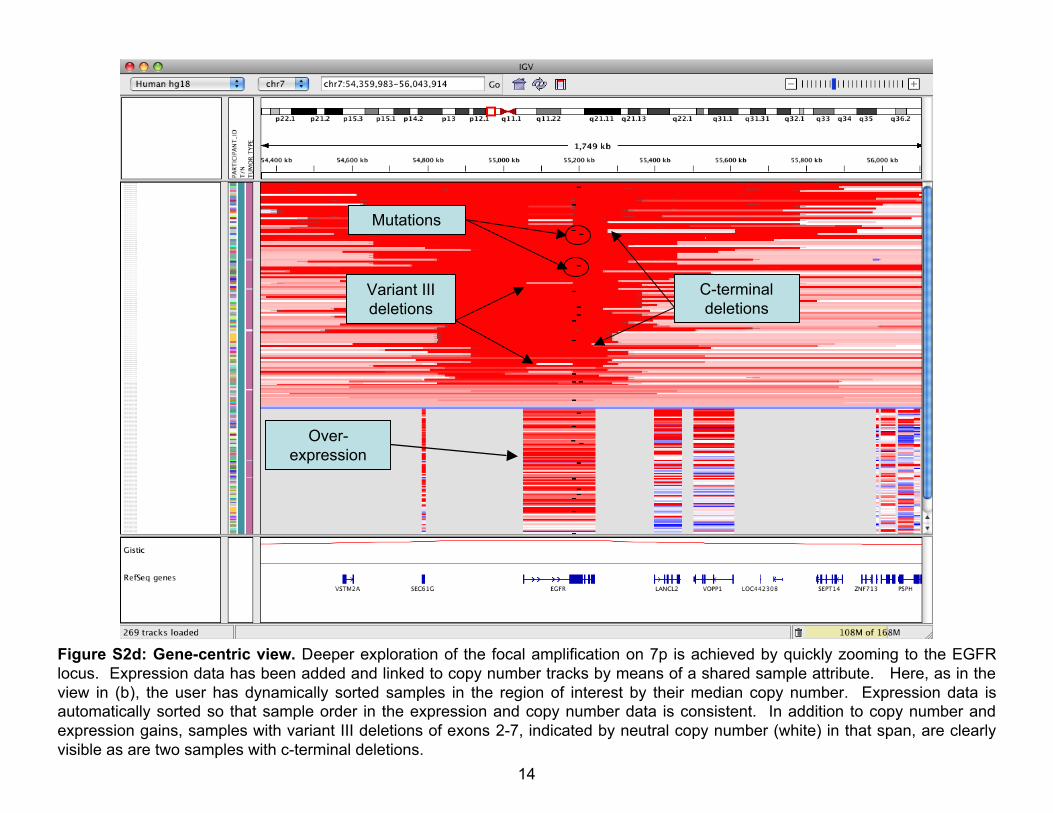
Mutations

Variant IIIdeletions

C-terminaldeletions

Over-expression

Figure S2d: Gene-centric view. Deeper exploration of the focal amplification on 7p is achieved by quickly zooming to the EGFRlocus. Expression data has been added and linked to copy number tracks by means of a shared sample attribute. Here, as in theview in (b), the user has dynamically sorted samples in the region of interest by their median copy number. Expression data isautomatically sorted so that sample order in the expression and copy number data is consistent. In addition to copy number andexpression gains, samples with variant III deletions of exons 2-7, indicated by neutral copy number (white) in that span, are clearlyvisible as are two samples with c-terminal deletions.

14

Sequence andamino acid

tracks

Mutations showing mutatedbase

Figure S2e: Individual base pair resolution view. Zooming to single base resolution provides the reference genomic sequenceand amino acids affected by these mutational events. Here we find two adjacent EGFR extracellular domain missense mutations.

15

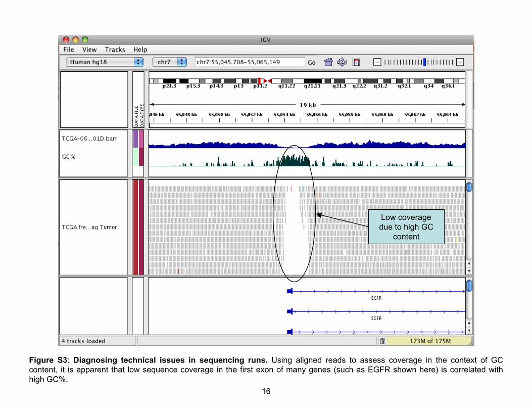
Low coveragedue to high GC

content

Figure S3: Diagnosing technical issues in sequencing runs. Using aligned reads to assess coverage in the context of GCcontent, it is apparent that low sequence coverage in the first exon of many genes (such as EGFR shown here) is correlated withhigh GC%.

16

Figure S4: Visualization of ChIP-Seq, RNA-Seq, and Conservation. Histone modification patterns, RNA levels, and conservationlevels are shown for a region. In green, H3K4me3 and in blue H3K36me3 are plotted as the number of DNA fragments obtained byChIP-Seq at each position across the genome. H3K4me3 marks the 5’ end of active genes while H3K36me3 marks the entireelongated transcript. The H3K4me3 peak is shown by the green box and the H3K36me3 region is shown with the blue box. Thisregion corresponds to a previously annotated protein coding gene which is shown at the bottom of the panel. RNA-Seq tracks (black)are displayed from the same cell types below the histone modifications. In addition to the processed reads, the locations of the rawgenome alignments are displayed in gray. The locations of these mapped reads coincide well with the previously determined exonicstructure of this gene. Finally, the phastCons evolutionary conservation score is plotted for each position in the genome is shown inblue.

17

A.

C.

B.

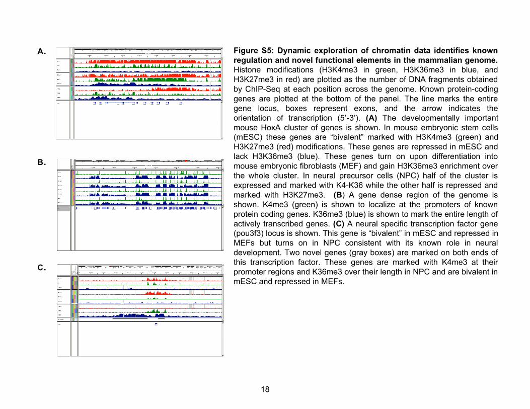
Figure S5: Dynamic exploration of chromatin data identifies knownregulation and novel functional elements in the mammalian genome.Histone modifications (H3K4me3 in green, H3K36me3 in blue, andH3K27me3 in red) are plotted as the number of DNA fragments obtainedby ChIP-Seq at each position across the genome. Known protein-codinggenes are plotted at the bottom of the panel. The line marks the entiregene locus, boxes represent exons, and the arrow indicates theorientation of transcription (5’-3’). (A) The developmentally importantmouse HoxA cluster of genes is shown. In mouse embryonic stem cells(mESC) these genes are “bivalent” marked with H3K4me3 (green) andH3K27me3 (red) modifications. These genes are repressed in mESC andlack H3K36me3 (blue). These genes turn on upon differentiation intomouse embryonic fibroblasts (MEF) and gain H3K36me3 enrichment overthe whole cluster. In neural precursor cells (NPC) half of the cluster isexpressed and marked with K4-K36 while the other half is repressed andmarked with H3K27me3. (B) A gene dense region of the genome isshown. K4me3 (green) is shown to localize at the promoters of knownprotein coding genes. K36me3 (blue) is shown to mark the entire length ofactively transcribed genes. (C) A neural specific transcription factor gene(pou3f3) locus is shown. This gene is “bivalent” in mESC and repressed inMEFs but turns on in NPC consistent with its known role in neuraldevelopment. Two novel genes (gray boxes) are marked on both ends ofthis transcription factor. These genes are marked with K4me3 at theirpromoter regions and K36me3 over their length in NPC and are bivalent inmESC and repressed in MEFs.

18

Low qualityalignments

Figure S6: Suspicious SNP call. This figure shows aligned reads from a region on Chromosome 2 derived from whole genomesequencing of a CEU (Western European ancestry) trio. Coverage depths are approximately 30x. Parents were sequenced on theIllumina platform. Three technologies were used for the child, Illumina (SLX), 454 and SOLID. A SNP in the CEU daughter wascalled by an analysis tool, however visual inspection raises several flags, (1) the SNP is not present in either parent, (2) there aremany nearby reads with mapping quality of zero, indicated by light grey shading with a darker outline, and (3) an unexpected (~5:1)allele imbalance in the SLX (Illumina) reads. Mousing over a feature or track reveals popup text – in this example supplyingadditional information for a read and the coverage plot. Note that one read is colored red, indicating that its mate is mapped toanother chromosome (chr20). This is confirmed in the popup text.

19

Figure S7: A de novo mutation in the CEU daughter. Another region, this one on Chromosome 1, from the same trio datasetdescribed in Figure S6. A heterozygous SNP is detected with ~50/50 allele balance in all three sequencing platforms for the CEUdaughter. Both read and alignment quality scores are high as indicated by the bright base letters and solid alignment features.The SNP is not present in either parent, indicating it is de novo.

20

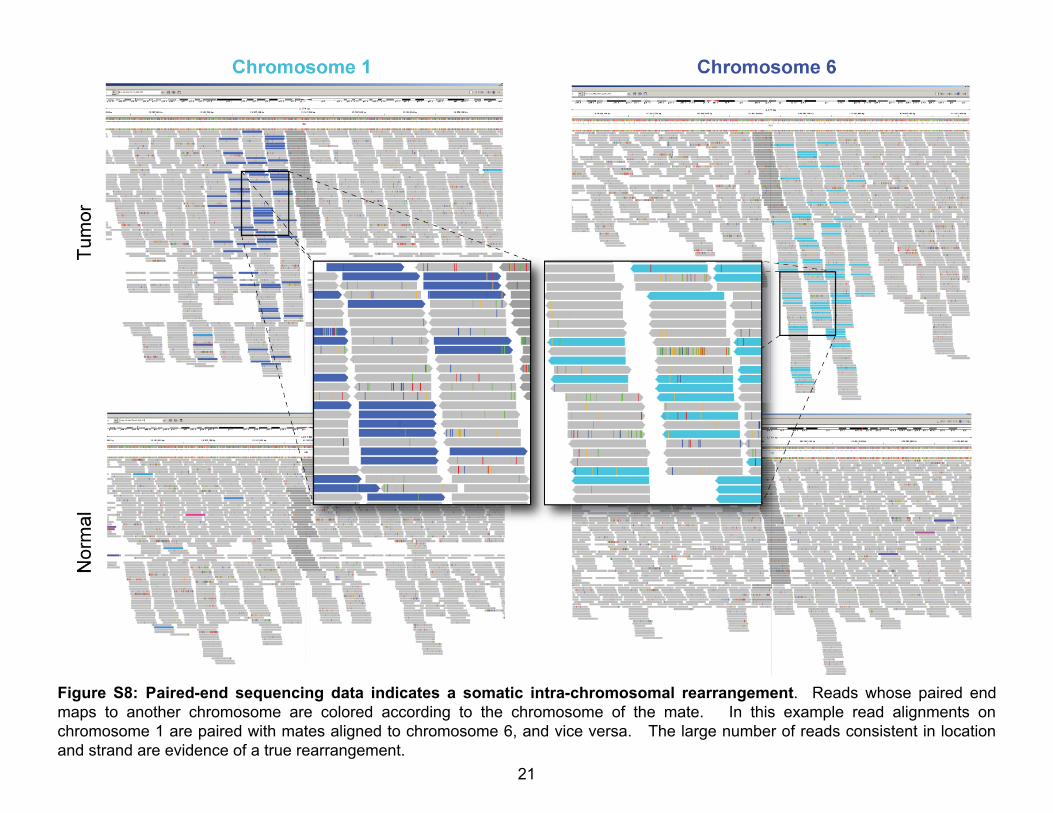
Figure S8: Paired-end sequencing data indicates a somatic intra-chromosomal rearrangement. Reads whose paired endmaps to another chromosome are colored according to the chromosome of the mate. In this example read alignments onchromosome 1 are paired with mates aligned to chromosome 6, and vice versa. The large number of reads consistent in locationand strand are evidence of a true rearrangement.

21

Rearrangements

Figure S9: Putative rearrangement flagged by analysis but rejected by visual inspection. This figure shows aligned readsfrom a whole genome scan of a glioblastoma multifome tumor sample. Although there are a few mate-pairs that are consistent inorientation, there are many more randomly scattered around the region. Also, there are a very high number of base mismatches fora 3 kb window, as indicated by the many colored bars in the coverage graph. Taken together, the evidence points to misalignmentsin this region rather than a true genomic event.

22

8/23/10 1:09 PMIGV User Guide

Page 1 of 58http://www.broadinstitute.org/igv/book/export/html/6

IGV User GuideThis guide fully describes the Integrative Genomics Viewer (IGV).

To start IGV, go to the IGV downloads page: http://www.broadinstitute.org/igv/download. For a 10-minute hands-on introduction, see the Quick Start.

User Interface

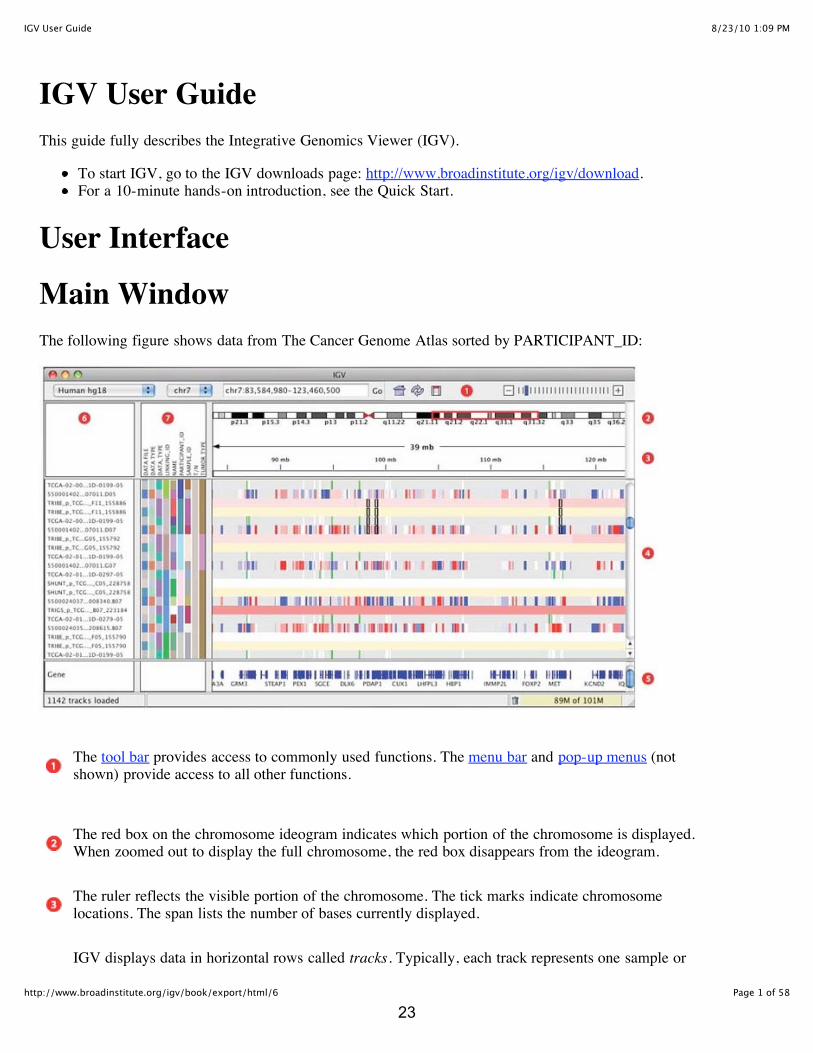
Main WindowThe following figure shows data from The Cancer Genome Atlas sorted by PARTICIPANT_ID:

The tool bar provides access to commonly used functions. The menu bar and pop-up menus (notshown) provide access to all other functions.

The red box on the chromosome ideogram indicates which portion of the chromosome is displayed.When zoomed out to display the full chromosome, the red box disappears from the ideogram.

The ruler reflects the visible portion of the chromosome. The tick marks indicate chromosomelocations. The span lists the number of bases currently displayed.

IGV displays data in horizontal rows called tracks. Typically, each track represents one sample or

23



experiment. This example shows methylation, gene expression, copy number, LOH and mutationdata.

IGV also displays features, such as genes, in tracks. By default, IGV displays data in one panel andfeatures in another, as shown here. Drag-and-drop a track name to move a track from one panel toanother. Combine data and feature panels by selecting that option on the General tab of thePreferences window.

Track names are listed in the far left panel. Legibility of the names depends on the height of thetracks; i.e. the smaller the track the less legible the name.

Attribute names are listed at the top of the attribute panel. Colored blocks represent attribute values,where each unique value is assigned a unique color. Hover over a colored block to see the attributevalue. Click an attribute name to sort tracks based on that attribute value.

Menu BarMenu Command Description

File Load from File Displays genomic data from one or more files. more...

Load from URL Displays genomic data from a file identified by URL. more...

Load fromServer

Displays genomic data from the IGV data server. more...

New Session Unloads all currently loaded data, as if you exited and restarted IGV. more...

Open Session Opens a previously saved session file. more...

Save Session Saves your current settings to a named session file. more...

Import Genome Imports a genome into IGV. more...

RemoveImportedGenomes

Removes an imported genome from the Genomes drop-down list in the toolbar. more...

Save ImageSaves a snapshot of the IGV window to a graphics file, omitting the menubar and tool bar.

Export RegionsSaves currently defined regions of interest to a BED file. If no regions ofinterest are defined, no BED file is created. more...

Import Regions Imports regions of interest from a BED file. more...

Clear Regions Removes all currently defined regions of interest. more...

24



Exit Closes IGV.

View Preferences Opens a tabbed menu of data display preferences. more...

Color Legends Displays color legends for track data, which may be modified. more...

Show AttributeDisplay

Shows/hides attributes and attribute values. more...

Select Attributesto Show

Shows/hides selected attributes and attribute values. more..

Refresh Refreshes the display.

Tracks Sort Tracks Sorts track data. more...

Group Tracks Groups track data. more...

Filter Tracks Filters track data. more...

Fit Data toWindow

Sets the track height to display all of the data, or as much data as possible.more...

Set TrackHeight

Sets the track height to a specified value. more...

Help Help Displays the IGV User Guide.

Tutorial Displays the IGV Quick Start.

About IGV Displays IGV version and build number.

Tool Bar

Genome drop-down boxLoads a genome. more...

Chromosome drop-down boxZooms to a chromosome. more...

Search box Displays the chromosome location being shown. To scroll to adifferent location, enter the gene name, locus, or track nameand click Go. more...

Whole genome viewZooms to whole genome view. more...

RefreshRefreshes the display.

25



Define a regionDefines a region of interest on the chromosome. more...

Zoom sliderZooms in and out on a chromosome. more...

Pop-up MenusTo select tracks and display the pop-up menu, do one of the following:

Right-click a track to select it and display the pop-up menu.Right-click an attribute value to select all tracks with that attribute value and display the pop-upmenu. Tip: Keep in mind that right-clicking an attribute may select tracks that are not visible in thedata panel. Scroll down the data panel to view all the selected tracks.Control-click track names (Mac: Command-click) to select the tracks, then right-click one of theselections to display the pop-up menu.

Commands in the track pop-up menu change the display options for the selected tracks. Most changesmade via the pop-up menu are lost when you exit IGV unless you save the session. In a few cases,changing the pop-up menu also changes an option in the Preferences window; these changes arepersistent.

The type of data displayed in the selected tracks determines which commands appear in the pop-up menu.This page lists commands by track type: data track, feature track, and alignment track. Use your browser'ssearch function to find a particular command.

Data Track

Data tracks display numeric values. For an example, click File > Load from Server and select The CancerGenome Atlas.GBM.Expression.GBM Batch 1-8 Centered and Normalized (hg18). The followingcommands appear in the pop-up menu for data tracks:

Command Description

Type of GraphHeatmapBar ChartScatterplotLine Plot

Changes the way IGV displays track data. more...

Windowing Function10th PercentileMedianMean90th PercentileMaximum

Changes the value represented by each pixel of track data.

At all but the lowest zoom levels, each pixel represents a significantamount of data. IGV divides the data to be displayed into "windows" ofequal length each corresponding to a single pixel, summarizes the valuesacross each window, and then displays the summarized values in thetrack. Select the function IGV will use to summarize the values.

26



Rename Track Renames a track. more...

Set Data RangeChanges the minimum, baseline, and maximum values of the graph usedto display track data. more...

Set Heatmap ScaleChanges the data range and color of the heatmaps used to display trackdata. more...

Change Track Height Changes the track height for selected tracks. more...

Change Track Color(Positive/Negative Values)

Changes the track color for selected tracks. more...

Remove Tracks Removes selected tracks from the display. more...

Feature Track

Feature tracks identify genomic features. For an example, see the Gene track, which IGV loads when youselect a genome. The following commands appear in the pop-up menu for feature tracks:

Command Description

Rename Track Renames a track. more...

Expand Track/Collapse Track

Displays overlapping features, such as different transcripts of a gene, onone line or multiple lines:

Collapsed state (default): Expanded state:

Change Track Height Changes the track height for selected tracks. more...

Change Track Color Changes the track color for selected tracks. more...

Remove Tracks Removes selected tracks from the display. more...

Alignment Track

Alignment tracks display alignments (more...). For an example, select the Human b36 genome, click File> Load from Server and select an alignment from the 1000 Genomes project. Tip: Zoom in to viewalignments and the alignment track pop-up menu.

27



Command Description

Sort alignmentsSorts alignments by start location, strand, nucleotide, mapping quality,sample, or read group (as defined in the BAM file).

Re-pack alignments Sorts alignments to minimize gaps at the top of the track.

Shade base by quality

Uses the color intensity of a mismatched base to indicate its qualityscore: the darker the color the higher the score. Changing this optionalso changes the option on the Alignments tab of the Preferenceswindow.

Shade alignmentsintersecting center

When selected, IGV shows a line at the center of the display and shadesalignments that intersect that center line. Changing this option alsochanges the option on the Alignments tab of the Preferences window.

Copy read details toclipboard

When you hover over a read, the tool tip displays information about theread. This option copies that information and the read sequence to theclipboard.

Go to mate region Jumps to the region of the paired read (if any).

Show all basesBy default, mismatched bases are displayed as colored letters on a graybar that represents the read. Select this option to display all bases in theread.

Show coverage trackWhen selected, IGV displays the matching coverage track for thealignment track.

Load coverage data

Loads coverage data for an alignment track. To generate coverage data,use igvtools. more...

Loading an alignment track from the IGV data server (File > Load fromServer) automatically loads the matching coverage data.

Rename track Renames a track.

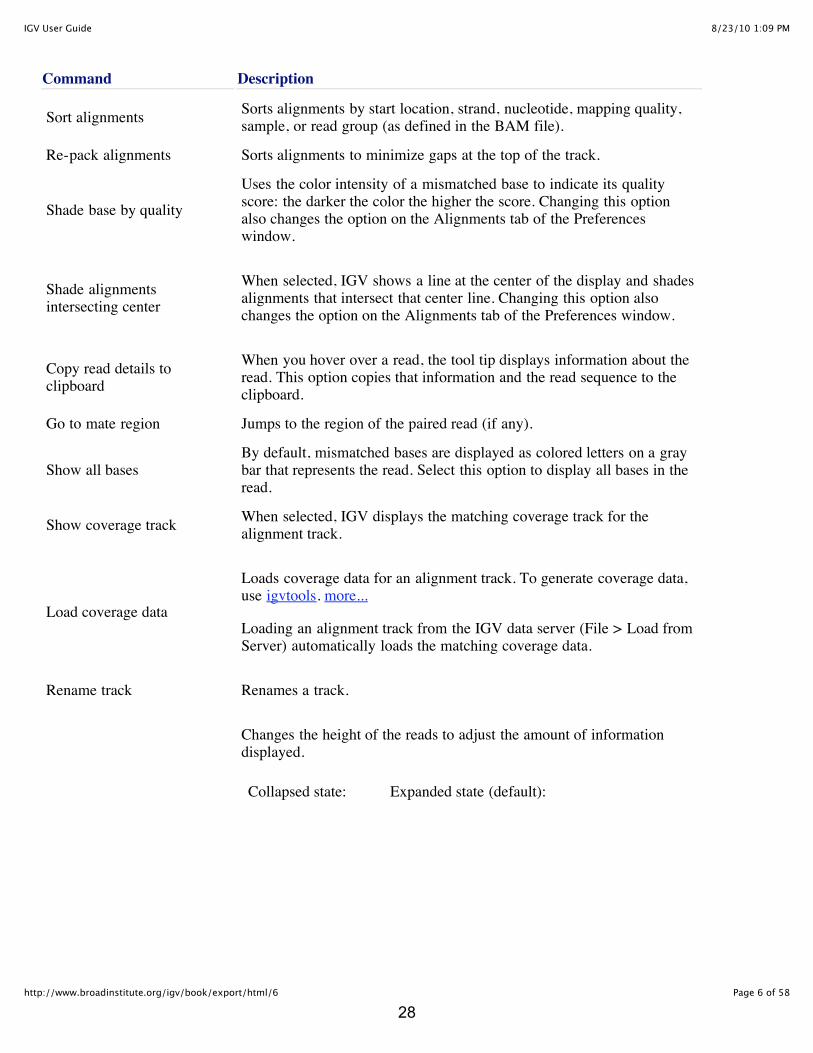
Changes the height of the reads to adjust the amount of informationdisplayed.

Collapsed state: Expanded state (default):

28



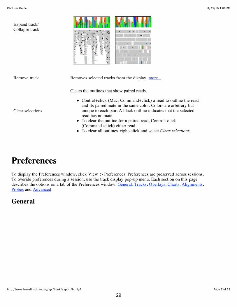
Expand track/Collapse track

Remove track Removes selected tracks from the display. more...

Clear selections

Clears the outlines that show paired reads.

Control+click (Mac: Command+click) a read to outline the readand its paired mate in the same color. Colors are arbitrary butunique to each pair. A black outline indicates that the selectedread has no mate.To clear the outline for a paired read, Control+click(Command+click) either read.To clear all outlines, right-click and select Clear selections.

PreferencesTo display the Preferences window, click View > Preferences. Preferences are preserved across sessions.To overide preferences during a session, use the track display pop-up menu. Each section on this pagedescribes the options on a tab of the Preferences window: General, Tracks, Overlays, Charts, Alignments,Probes and Advanced.

General

29



Select to distinguish regions with zero values (white) from regions with missing data (gray). Clear(default) to display both regions in the same way (gray). Effects only bar charts and scatter plots.

Select to display all tracks in a single panel. Clear (default) to display data tracks (e.g., expressiondata) in one panel and feature tracks (e.g., genes) in another.

Select (default) to fill the gaps between adjacent segments by extending the segment endpoints.Clear to leave gaps between adjacent copy number segments. Effects only tracks displayingsegmented copy number.

Select (default) to show attributes and attribute values to the left of the data panel. Clear to hide theattributes. This option and View > Show Attribute Display have the same effect on attributedisplay.

Zoom to feature (not shown). When selected the zoom level is automatically adjusted so that thetarget feature fills the view after a successful search. If not checked the target feature of a search iscentered in the view but the zoom level is unaffected.

Tracks

30



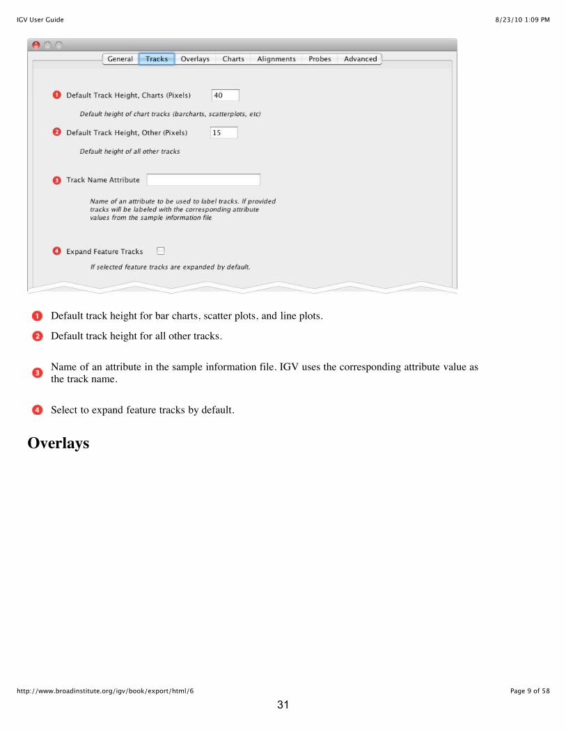
Default track height for bar charts, scatter plots, and line plots.

Default track height for all other tracks.

Name of an attribute in the sample information file. IGV uses the corresponding attribute value asthe track name.

Select to expand feature tracks by default.

Overlays

31



Select to overlay mutation data on other tracks. more...

Name of an attribute in the sample information file. IGV uses the corresponding attribute value to"link" mutation data with other track data. more...

Select to color-code mutation data overlaid on other tracks. Click Choose Colors (or View > ColorLegends) to display the Color Legends window, which allows you to view and change mutationcolor codes. more...

When mutation data is displayed in a separate track, IGV color codes mutations by type (missense,silent, and so on). By default, when mutation data is overlaid on other tracks, IGV displaysmutations in black for clarity.

Select to display mutation data in a separate track. more...

Charts

32



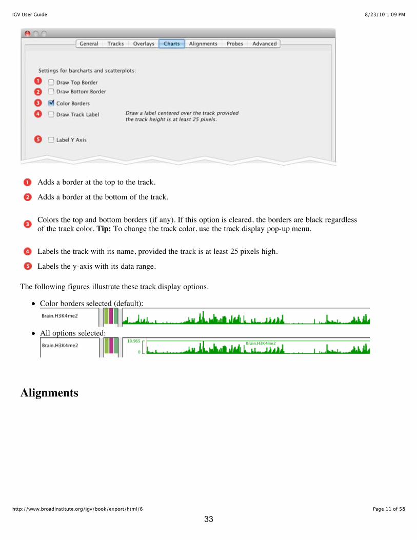
Adds a border at the top to the track.

Adds a border at the bottom of the track.

Colors the top and bottom borders (if any). If this option is cleared, the borders are black regardlessof the track color. Tip: To change the track color, use the track display pop-up menu.

Labels the track with its name, provided the track is at least 25 pixels high.

Labels the y-axis with its data range.

The following figures illustrate these track display options.

Color borders selected (default):

All options selected:

Alignments

33



Sets the threshold at which IGV displays reads. Reads are visible only when IGV is zoomed in todisplay a number of bases less than or equal to this threshold.

Sets the maximum number of vertically stacked alignments viewable at any particular locus.

Sets a threshold on alignment mapping quality. Only alignments with mapping quality greater thanor equal to this threshold are shown.

Sets a size threshold for the flagging of paired end alignments. Only paired end alignments withinsert sizes greater than or equal to this threshold are flagged.

Select to display alignments marked as duplicate reads.

Select to draw a red box around any paired alignment whose mate is not mapped.

Select to display a coverage track for each alignment track. The coverage track is visible only whenalignments are visible. It displays a gray bar chart showing the depth of the reads at each locus. If anucleotide differs from the reference sequence in greater than 20% of quality weighted reads, IGVcolors the bar in proportion to the read count of each base (A, C, G, T). Modifying this optionaffects the display of subsequently loaded alignment tracks.

Select to display the reference sequence with each alignment track. When cleared (default), IGV

34



displays the reference sequence once. Modifying this option affects the display of subsequentlyloaded alignment tracks.

Select to display a line at the center of the display. When zoomed in sufficiently, IGV shadesalignments that intersect the center line. At higher resolutions, the center line becomes lines thatframe the aligned bases at the center of the display. Modifying this option affects the display ofsubsequently loaded alignment tracks.

Hide alignments that match the read groups listed in the filter file. The filter file is a text file thatlists read groups one per line.

A colored read indicates a paired end read with a mate on another chromosome. The color of theread indicates which chromosome holds its mate.

Probes

Choose an option to determine how IGV places expression data on the genome:

Map probes to target loci: Use the probe ID to determine the probe locus and display data at thatlocation. If that fails, map the probe ID to a gene, determine the gene locus, and display data at thatlocation.

Map probes to genes: Map the probe ID to a gene, determine the gene locus, and display data atthat location.

Modifying this option affects the display of subsequently loaded alignment tracks.

Advanced

35



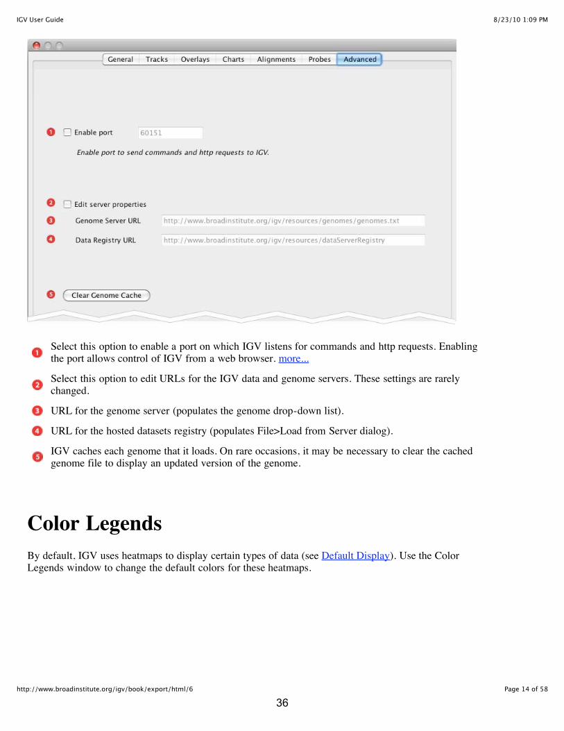
Select this option to enable a port on which IGV listens for commands and http requests. Enablingthe port allows control of IGV from a web browser. more...

Select this option to edit URLs for the IGV data and genome servers. These settings are rarelychanged.

URL for the genome server (populates the genome drop-down list).

URL for the hosted datasets registry (populates File>Load from Server dialog).

IGV caches each genome that it loads. On rare occasions, it may be necessary to clear the cachedgenome file to display an updated version of the genome.

Color LegendsBy default, IGV uses heatmaps to display certain types of data (see Default Display). Use the ColorLegends window to change the default colors for these heatmaps.

36



To change the default colors:

1. Click View > Color Legends to display the Color Legends window.2. Click a heatmap legend to set its color and range.3. For LOH and Mutation data, click a colored box to change its color.

Navigating

Zooming

Zoom out to view the whole genome, zoom in to a chromosome and continue zooming to base pairresolution. As you zoom in, the gene track shows gene names and sequence data. If the sequence data isunavailable, small blocks replace the bases. If you are using a genome stored on the IGV genome server,you must be connected to the internet to view the sequence data.

Click the whole genome view icon to zoom out to the genome view.

37



From the genome view, zoom to a chromosome by clicking its label.

Select a chromosome from the drop-down menu to zoom to it.

To zoom in and out on a chromosome:

Zoom in Zoom out

+ -

Double-click or shift-click the track data Alt-click (Mac: option-click) the track data

Click a zoom level on the zoom slider Click a zoom level on the zoom slider

Click the plus (+) icon on the zoom slider Click the minus (-) icon on the zoom slider

Scrolling

To scroll the display:

Vertical scroll Horizontal scroll*

Scroll bar in the IGV window Click and drag the track data

Click and drag the track data Click the chromosome ideogram to scroll to that location

Page Up and Page Down keys Click the ruler to center that location

Up and down arrow keys Left and right arrow keys

Home and End keys (scroll by screen width)

* You cannot scroll horizontally when IGV is displaying the whole genome or a whole chromosome.

Searching

Use the search box to locate:

A locus (for example, chr5:90,339,000-90,349,000)A gene symbol or other feature identifier (e.g., DPYD or NM_10000000)A track name (e.g., secondary_GBM_89)

IGV searches for an exact match to the name entered in the search box. For example, entering 'secondary'will not locate the 'secondary_GBM_89' track. If multiple features have the same name, IGV jumps to anarbitrary match.Ju

Jumping

If you have a feature track loaded (e.g. Gene track, BED or GFF file), you can jump from one feature to

38



the next.

1. Click the track that contains the features that you want to find.2. Jump from feature to feature:

Click Ctrl+F to jump forward to the next feature.Click Ctrl+B to jump backward to the previous feature.

IGV positions the start of the next (or previous) feature at the center of the display.

Loading a GenomeIGV displays annotations for one genome at a time. To load a different genome, select it from thegenome drop-down list in the tool bar:

When you switch genomes, IGV does not remap data that has already been loaded. We recommendthat you remove loaded tracks (File>New Session), switch genomes, and then load the desired datafiles.The genome selected when IGV exits is automatically selected when IGV restarts.

Selecting a Hosted Genome

IGV provides several genomes, which are hosted on a server at the Broad Institute. Initially, the genomedrop-down lists only these hosted genomes. If the genome you need is not available, either contact [email protected] and request that it be added or import the genome.

Importing a Genome

If the genome drop-down list does not include the genome that you need, you can easily import it.Imported genomes appear at the top of the genome drop-down list, above the hosted genomes.

Prerequisites:

A FASTA file , directory of FASTA files, or zip of FASTA files that contains the sequence data foreach chromosome in the genome. (Required)A cytoband file, which IGV uses to display the chromosome ideogram. (Optional)An annotation file in BED file format, the GFF file format, or any variation of the genePred tableformat. (Optional)

Step-by-step:

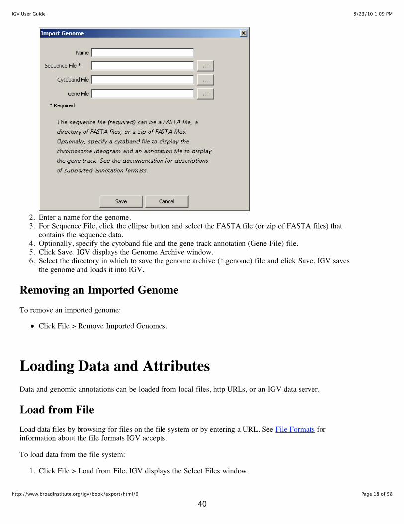
1. Click File > Import Genome. IGV displays the Import Genome window:

39



2. Enter a name for the genome.3. For Sequence File, click the ellipse button and select the FASTA file (or zip of FASTA files) that

contains the sequence data.4. Optionally, specify the cytoband file and the gene track annotation (Gene File) file.5. Click Save. IGV displays the Genome Archive window.6. Select the directory in which to save the genome archive (*.genome) file and click Save. IGV saves

the genome and loads it into IGV.

Removing an Imported Genome

To remove an imported genome:

Click File > Remove Imported Genomes.

Loading Data and AttributesData and genomic annotations can be loaded from local files, http URLs, or an IGV data server.

Load from File

Load data files by browsing for files on the file system or by entering a URL. See File Formats forinformation about the file formats IGV accepts.

To load data from the file system:

1. Click File > Load from File. IGV displays the Select Files window.

40



2. Select one or more data files or sample information files, then click OK. CTRL-click (Mac:Command-click) to select multiple files.

Load from URL

To load data from an HTTP URL:

1. Click File > Load from URL.2. Enter the HTTP URL for a data file or sample information file, then click OK.

Notes:

The following file types cannot be loaded by URL at this time: .sam, .sorted.txt, .h5 (superseded by.tdf) and .aligned (internal Broad format).FTP is not supportedFor .bam, .tdf, and indexed file formats the server must support byte-range requests.

Load from Server

To load data from the IGV data server:

1. Click File > Load from Server. The Available Datasets window appears:

2. Expand the tree to see the datasets.3. Select one or more datasets. Click the check box to the left of a dataset to select it.

Warning: Selecting a folder selects all of its subfolders and all of the datasets in those folders. Thiscan potentially be a huge amount of data. To be sure you are loading only the data you want, opencollapsed folders and select only the datasets of interest.

4. Click OK. IGV displays the genomic data.

Removing Tracks and Attributes

To remove all tracks and attributes:

Click File > New Session. This is essentially the same as restarting IGV.

41



To remove specific tracks, do one of the following:

Right-click a track name and click Remove Tracks in the pop-up menu.Right-click an attribute value, which selects all tracks tagged with that attribute value, and clickRemove Tracks in the pop-up menu.Control-click track names (Mac: Command-click), then right-click one of the selections and clickRemove Tracks in the pop-up menu.

Note:

Sequence data is associated with the gene track; therefore, removing the gene track removes thesequence data.You cannot remove individual attributes during a session, but you can hide them.

Viewing AttributesAttributes can be associated with tracks and used for filtering, sorting, and grouping data. By default alltracks have at least 3 attributes: Data File, Data Type, and Name. To display additional attributes, load asample attribute file. IGV displays attribute names and values in the attributes panel.

Color-Coded Attribute Values

IGV uses color-coded blocks to represent the attribute values.

Hover over a colored block to display the attribute value.Click a colored block to select all tracks with that attribute value. IGV indicates a selected track byhighlighting the track name. Tip: Keep in mind that clicking an attribute may select tracks that arenot visible in the data panel. Scroll down the data panel to view all the selected tracks.

Showing and Hiding Attributes

42



To show or hide selected attributes:

1. Click View > Select Attributes to Show. IGV displays a list of attributes.2. Select (or clear) an attribute’s check box to show (or hide) the attribute.3. Click OK. IGV updates the display to show only the selected attributes.

To show or hide all attributes:

Click View > Show Attribute Display to toggle the setting. A check mark next to the menu itemindicates that the attribute panel is displayed. No check mark indicates that it is hidden. Tip: This is a persistent setting. Toggling the menu item also toggles the corresponding setting onthe General tab of the Preferences window and vice versa.

Viewing Data

Default DisplayWhen you load genomic data, IGV displays the data in horizontal rows called tracks. Typically, eachtrack represents one sample or experiment. For each track, IGV displays the track identifier, one or moreattributes, and the data.

When loading a data file, IGV uses the file extension to determine the file format (see File Formats), thefile format to determine the data type (Table 1), and the data type to determine the track default displayoptions (Table 2).

File Format Data TypeTable 1. File Format Determines Data Type

CBS, CN, SEG, SNP Copy number

LOH LOH

GCT Gene expression or RNAi

43



GISTIC GISTIC data

RES Gene expression

SAM, BAM Sequence alignments

BED, GFF, GFF3 Genome annotations

MUT Mutation

IGV, WIG, HDF5 file not created withalignment processor

Other

Cytoband, FASTANot applicable. Cytoband and sequence files for animported genome.

Data Type Default Graph Type Default Data Range Default ColorsTable 2. Data Type Determines Display Options

Copy number Heatmap -1.5 to 1.5 Blue to red

Gene expression Heatmap -1.5 to 1.5 Blue to red

Chip Bar chart None, data is autoscaled Blue

DNA methylation Heatmap0 to 1(methylation score)

Green

Allele-specific copy number Heatmap -1.5 to 1.5 Blue to red

LOH Heatmap -1 to 1Blue = LOH (1)Yellow = Retained (0)Red = Conflict (-1)

RNAi Heatmap -3 to 3 Red to blue

Other Bar chart None, data is autoscaled Blue

Changing the DisplayYou can override IGV's default display options in several ways:

Use the track pop-up menu to change the appearance of selected tracks. Use the Preferences window to set display preferences for all tracks.Use the Color Legends window to set the default data range and color for heatmaps, whichIGV uses to display copy number, gene expression, RNAi, methylation, LOH, and mututation data(Table 2).For IGV and segmented (SEG, CBS) data files, add a type line to the data file to override thedefault data type associated with the file format and thus the default display options for the data.Add a track line at the top of a data file to specify the display settings for the data.Override the default display settings by including display attributes in the sample information file.Note that changes made with this method take precedence over the defaults prescribed by a #typeline.

44



This section describes a few commonly used display options that apply to all (or most) tracks: graph type,data range, track color, track height, andtrack names. For information about how to load and displayspecific types of data, see Viewing Data. For a complete list of display options, review the optionsavailable in the pop-up menus, Preferences window, Color Legends window, and the menu bar (View andTracks menus).

Graph Type

Most tracks are displayed using one of four graph types (the following graphs show the same data):

Heatmap:

Barchart:

Scatterplot:

Lineplot:

IGV determines the default graph type for a track as described in Default Display.

To change the graph type of selected tracks:

Right-click a track and select a graph type from the pop-up menu.

Data Range

The data range for a track provides the minimum, baseline, and maximum value for the graph. IGVdetermines the default data range for a track as described in Default Display.

To change the data range for selected heat map tracks:

Right-click a track and select Set Heatmap Scale from the pop-up menu.

To change the data range for other selected tracks:

Right-click a track and select Set Data Range from the pop-up menu.

Changing the data range can significantly affect the data display:

minimum,baseline,maximum

Result

45



0,0,3

-1.5,0,1.5

-5,0,5

Track Color

To change the track color for selected heat map tracks:

Right-click a track and select Set Heatmap Scale from the pop-up menu.

To change the track color for other selected tracks:

Right-click a track and from the pop-up menu select either Change Track Color (Positive Values)or Change Track Color (Negative Values).

Track Height

To change the height of selected tracks:

Use the track pop-up menu.

To change the height of all tracks:

Click Tracks > Set Track Height and enter a value.

To fit the data to the window:

Click Tracks > Fit to Window. IGV displays all tracks. If necessary, it sets the track height to 1 pixel and scrolls the data.

Track Names

By default, IGV displays track names to the left of the attribute panel. Legibility of the track namesdepends on track height; for example, track names will not be legible when track height is 1 pixel).

To select the attribute IGV uses as the track name:

Use the Tracks tab of the Preferences window.

To display the track name as a track label:

Use the Charts tab of the Preferences window.

To rename a track:

46



Right-click a track or a track name, then click Rename Track in the pop-up menu.

You can only rename one track at a time. You can preserve track name changes only by saving thesession.

Expanding the Track

By default all features in a track are drawn on a single line, including features that might overlap such asalternative isoforms of a transcript.

To see all overlapping features right-click on the feature track and select Expand Track.

This breaks expands the track to multiple rows as required so that features do not visibly overlap.

Expression Data

File Formats

For expression data, use the GCT file format. This a tab-delimited format that contains a row for eachprobe set ID (or gene), a column for each sample, and expression values for each feature in each sample.

Display Notes

By default, IGV displays expression data as a blue-to-red heatmap where the data range is -1.5 to1.5. If loaded expression data appears in tracks colored all red, check the data values and modifythe data range as necessary.To change track display options, use the track pop-up menu. The commands that appear in the pop-up menu are those relevant to any data track.

Genomic Locations for Probes

To display expression data, IGV must first map the probe set IDs named in the expression data file to

47



their genomic locations. IGV displays data for all of the probes that it can map to genomic locations. Ifnone of the probes in the file can be mapped, IGV displays an error message.

IGV determines the genomic locations for probes as follows:

1. If you use the delimiters |@ and | to specify the probe loci in the file (see the GCT file format), IGVuses the specified loci. Otherwise, it goes to the next step.

2. IGV searches all loaded annotation tracks for each probe. (This is the same as entering the ID in thefirst column (the Name column) of the file into the search box on the IGV tool bar and clickingGo.) If a probe is found, IGV displays the data at that location. Otherwise, it goes to the next step.

3. IGV searches its probe mapping files for each probe. If a probe is found, IGV determines the probelocus and displays the data at that location. Otherwise, it goes to the next step.

4. IGV uses its gene mapping files to map each probe ID to a gene symbol, determines the genelocus, and displays the data at that location.

Choose preferred mapping: By default, IGV uses its probe mapping files before its gene mapping files.If you prefer to map probes to genes, select the 'Map probes to genes' radio button on the Probes tab ofthe Preferences window.

Probe Mapping Files

Probe mapping files map probe identifiers to chromosomal locations. They are compiled from source filesprovided by Affymetrix, Agilent, and Illumina. The Affymetrix and Agilent mapping files are split byspecies due to their large size. Separate mapping files are provided for human, mouse, and other (non-mouse, non-human) species. Human probe identifiers are mapped to hg18. Depending on the vendor,mouse probe identifiers are mapped to mm9 (Affymetrix), mm5 (Agilent) or mm8 (Illumina).

Following are links to the probe mapping files:

http://www.broadinstitute.org/igv/resources/probes/affy/affy_human_mappings.txt.gzhttp://www.broadinstitute.org/igv/resources/probes/affy/affy_mouse_mappings.txt.gzhttp://www.broadinstitute.org/igv/resources/probes/affy_other_mappings.txt.gzhttp://www.broadinstitute.org/igv/resources/probes/agilent/agilent_human_mappings.txt.gzhttp://www.broadinstitute.org/igv/resources/probes/agilent/agilent_mouse_mappings.txt.gzhttp://www.broadinstitute.org/igv/resources/probes/agilent/agilent_other_mappings.txt.gzhttp://www.broadinstitute.org/igv/resources/probes/illumina/illumina_allMappings.txt.gz

Gene Mapping Files

Gene mapping files map probe identifiers to gene identifiers. Following are links to the gene mappingfiles:

http://www.broadinstitute.org/igv/resources/probes/affy/affy_probe_gene_mapping.txt.gzhttp://www.broadinstitute.org/igv/resources/probes/agilent/agilent_probe_gene_mapping.txt.gzhttp://www.broadinstitute.org/igv/resources/probes/illumina/illumina_probe_gene_mapping.txt.gz

Sources for the Mapping Files

The probe and gene mapping files are compiled from source files provided by Affymetrix, Agilent, andIllumina. A list of the source files is available athttp://www.broadinstitute.org/igv/resources/probes/data_sources_for_mapping.txt.

48



Mutation Data

File Formats

Mutation data is loaded from a .mut file. The resulting values can be visualized as distinct tracks oroverlaid on other associated tracks (e.g. expression or SNP data from the same patient). This associationis specified by means of a special "linking" column in a sample information file. By default IGV looksfor a column with the heading LINKING_ID for this association, but the exact heading is configurable asa user preference under the Overlays tab. Mutations are overlaid on another track when the values of thiscolumn are equal. A typical use case is to record an identifier identifying a patient, or sample, in thiscolumn.

To visualize mutation data:

1. Format mutation data using the MUT file format; e.g. example.mut.2. Format the data from platform-specific assays using an appropriate file format; e.g. example.gct

(expression data) and example.seg (segmented copy number data).3. Define attributes and their values in a sample information file; e.g.

example_sampleinfo_LINKING_ID.txt. A sample information file contains a row for each trackand a column for each attribute:

The first column contains track identifiers. The track identifier for each mutation track andeach associated data track must be included in the sample information file. The trackidentifiers can be found in the data files (e.g. example.mut, example.gct and example.seg).

Each subsequent column identifies an attribute and its value (if any) for each track. IGVuses the value of one attribute (by default, LINKING_ID) to link mutations to associateddata tracks; a mutation track and data track that have the same value for this attribute arelinked.

49



In the example sample information file, the LINKING_ID attribute (2nd column) links the mutation anddata tracks. However, in practice, it might be easier to use an existing an attribute rather than adding aLINKING_ID attribute. Notice that, in this example, the LINKING_ID and Sample attributes have thesame value. The LINKING_ID attribute could be removed from the sample information file and theSample attribute used to link the mutation and data tracks. By default, IGV uses the LINKING_ID tooverlay mutations on data tracks. If you use an attribute other than LINKING_ID, enter that attributename on the Overlays tab of the Preferences window.

Display Notes

By default, IGV displays mutations (variant bases) in distinct tracks and overlaid on associated datatracks. Mutations displayed in distinct tracks are color coded by type (missense, silent, and so on).Mutations overlaid on data tracks are colored black for clarity.

Use the Color Legends window to view or change the mutation color codes.

Use the Overlays tab of the Preferences window to modify other display options for mutations.

50



RNAi DataIGV displays RNAi data similarly to expression data, with one exception: to facilitate analysis of hairpinscores, IGV provides a unique RNAi bar chart. To display the bar chart:

Right-click an RNAi track and select Bar Chart from the pop-up menu.

The following figure explains how to read the bar chart.

Hover over a track to view hairpin values.

51



Segmented Data

File Format

For segmented data, use the SEG or CBS file format.

Display Notes

By default, IGV displays segmented data as a blue-to-red heatmap where the data range is -1.5 to1.5. If loaded segmented data appears in tracks colored all red, check the data values and modifythe data range as necessary.To change track display options, use the track pop-up menu. The commands that appear in the pop-up menu are those relevant to any data track.

Gaps Between Segments

By default, IGV fills the gaps between adjacent segments by extending the segment endpoints. Whenzoomed in sufficiently, error bars indicate the gaps:

Alternatively, you can leave the gaps between the segments. In this case, the gaps appear gray:

To modify how gaps are displayed between adjacent segments set the "Join Adjacent CopyNumberSegments" option on the General tab of the Preferences window.

Viewing Alignments

File Formats

The preferred file format for viewing alignments in IGV is the BAM format, a binary form of SequenceAlignment Format (SAM). Both BAM and SAM files are described on the Samtools project pagehttp://samtools.sourceforge.net/. IGV requires that BAM files be indexed.

For large alignment files we recommend using the BAM format. However, SAM files can be usedprovided the alignments are sorted by start position and indexed. The igvtools command line utilities canbe used to both sort and index the files. Alternatively, if the file is already sorted an index will beautomatically created upon first loading the file. IGV will attempt to store the index in the directory

52



where the alignment file resides with an extension of ".sai". If that fails the index is stored in the usersIGV directory.

Alignments Panel

IGV displays sequence alignment data in a separate Alignments panel. The display changes as you zoomin. When zoomed out, IGV displays only coverage data, when available (more detail below).

When zoomed in to the alignment read visibility threshold (by default, 30 KB), IGV shows the reads. Atthis resolution the colored bars in the coverage track identify loci where more than 20% of the qualityweighted reads differ from the reference. For paired end alignments, reads that have a larger thanexpected insert size or a mate on another chromosome are color coded to indicate the chromosome of themate pair. (more detail below).

At higher resolutions read bases that do not match the reference are color coded, and insertions ( ),deletions relative to the reference become visible. By default, read bases that match are displayed ingray. To color code all bases, regardless of whether they are mismatched, right-click the track and selectShow All Bases from the pop-up menu. In addition, mismatched bases are assigned a transparency valueproportional to the read quality (phred) score. This has the effect of de-emphasizing low quality reads. Transparency shading can be turned off temporarily from the pop-up menu, or permanently from thePreferences window.

53



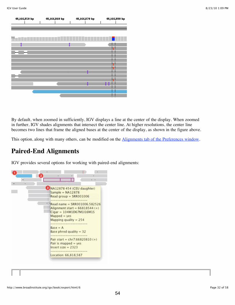
By default, when zoomed in sufficiently, IGV displays a line at the center of the display. When zoomedin further, IGV shades alignments that intersect the center line. At higher resolutions, the center linebecomes two lines that frame the aligned bases at the center of the display, as shown in the figure above.

This option, along with many others, can be modified on the Alignments tab of the Preferences window.

Paired-End Alignments

IGV provides several options for working with paired-end alignments:

54



IGV colors paired-end alignments whose inferred insert size is larger than expected or whose materead is aligned to a different chromosome. A read with a mate aligned to a different chromosome iscolor-coded to identify the other chromosome. A read with a large insert size is the color of its ownchromosome. The chromosome color legend is on the Alignments tab of the Preferences window:

Control+click (Mac: Command+click) a read to outline the read and its paired mate in the same color.Colors are arbitrary but unique to each pair. A black outline indicates that the selected read has nomate.

Control+click (Command+click) either read to clear the outline.Right-click and select Go to Mate Region to jump to the paired mate. Note: If the paired readshave a large insert size, the paired mate will not be highlighted. This is a known issue that willbe addressed in a future release.Right-click and select Clear Selections to clear all outlines.

Hover over a read to view information about the read, including the location of its paired mate.

Insertions

When viewing a gapped alignment, IGV indicates insertions with respect to the reference with a purplebar ( ). Hover over the insertion symbol to view the inserted bases.

Read Coverage

Default Coverage Data

IGV supplements each alignment track with a coverage track. When IGV is zoomed in sufficiently todisplay alignments, the coverage track displays the depth of the reads displayed at each locus as a graybar chart. If a nucleotide differs from the reference sequence in greater than 20% of quality weightedreads, IGV colors the bar in proportion to the read count of each base (A, C, G, T).

55



To hide the coverage track, clear the Show Coverage Track option on the Alignments tab of thePreferences window.

Extended Coverage Data

To display coverage data at the whole genome or chromosome level, use the igvtools package (countcommand) to generate coverage data for the alignments file. The resulting file can be associated with thealignment track by file naming convention, or loaded independently as a separate track.

To associate a coverage track using filename the track must be named as follows, and placed in the samedirectory as the alignment track:

<alignment file name>.tdf

For example, the coverage track for test.bam would be named test.bam.tdf.

To dynamically associate coverage data with a bam track choose the "Load Coverage Data" from eitherthe alignment or coverage track menu. When the alignment data is loaded with its matching coveragedata, the coverage track displays data at all zoom levels.

Sorting Alignments

Alignments can be sorted by start location, strand, nucleotide, mapping quality, sample, or read group.

To sort alignments:

1. Right-click a track to display the pop-up menu.2. Choose a Sort option from the menu. IGV sorts the alignments that intersect the center line of the

display.

Sorting rearranges rows so that alignements that intersect the center appear in the order specified. Thiscan cause the alignment layout away from the center line to appear sparse. To restore the layout to anoptimally packed configuration choose "Re-pack alignments" from the popup-menu.

56



Illumina Sequencing Support

IGV includes limited support for viewing alignments in the "sorted.txt" format from the Illumina Pipelineversion 1.3, with the following restrictions.

The contig fields (columns 12 and 19) are not supportedThe Match chromosome field (column 11) must either be the name of a chromosome in an IGVgenome, or an entry in the seqname to chromosome mapping file defined below.

Mapping File: To view alignments from a sorted.txt file in which the chromosome names are notchromosome names in IGV a mapping file must be provided. This is a 2 column tab delimited file withchromosome names from the sorted.txt file in column 1, and corresponding IGV chromosome names incolumn 2. The file must be named "sequence.map" and placed in a specific directory, which is platformdependent:

Windows: <user home>/igv/samLinux: <user home>/igv/samMac: <user home>/.igv/sam

On Windows computers the user home directory is normally found at

C:/Documents and Settings/<user name>

Sorting, Grouping, and FilteringBy default, IGV displays tracks in the order in which they are loaded (i.e. the order of the data in thefiles). Alternatively, sort the tracks by attribute, region of interest, or track list. You can also group orfilter tracks.

Sorting by Attribute

If tracks are grouped, IGV sorts the tracks in each group. To sort groups by attribute, first sort theungrouped tracks by the desired attributes, then group the tracks.

To sort tracks based on an attribute value:

Click the attribute name in the attributes panel. IGV sorts the tracks based on the attribute's value.

Alternatively, use the Sort Tracks command for additional options:

1. Click Tracks > Sort Tracks. IGV displays the Sort window:

57



2. Select the attributes to sort by and whether to sort based on ascending or descending values.

Sorting by Region of Interest

If tracks are grouped, IGV sorts the tracks in each group. It then sorts the groups using a composite scorefor the group, which IGV defines as the maximum score from the tracks in that group.

To sort tracks in the data panel based on a region of interest:

1. Define a region of interest on the genome, as shown below.2. Click the red bar above the defined region and select an option from the pop-up menu:

Sort by amplification: Affects tracks of copy number data. Sorts tracks based on copy numbervalues in this region, from highest to lowest.Sort by deletion: Affects tracks of copy number data. Sorts tracks based on copy numbervalues in this region, from lowest to highest.Sort by expression: Affects tracks of gene expression data. Sorts tracks based on geneexpression in this region, from highest to lowest.Sort by value: Sorts tracks based on the values of the track data in this region, from highest tolowest.Delete: Removes this region-of-interest annotation.

Defining Regions of Interest

A region of interest is a portion of the data panel that is highlighted with black lines at either side of theregion and a red bar at the top:

58



To define a region of interest:

1. In the tool bar, click the Define a Region icon:

2. In the data panel, click the start of the region and then the end of the region. IGV draws linesdelimiting the region.

To remove one region of interest from the display:

Right-click the red bar above the region and click Delete.

To remove all regions of interest from the display:

Click File > Clear Regions.

To export a region of interest:

Click File > Export Regions and save the file.

To import a region of interest:

Click File > Import Regions, navigate to the location of the exported file, and double-click it. IGVdisplays the lines delimiting the region.

Sorting and Filtering by Track List

To display selected tracks in a specific order:

1. Create a sample information file that contains two columns. The first column must be labeled'Array' and lists the tracks that you want to display. The second column can be labeled 'Order' (orany other label) and lists the sort order for the tracks.For example, the following sample information file provides a track list for use withsegmented_data_080520.seg:

Array Order

primary_GBM_10 a

primary_GBM_20 b

primary_GBM_30 c

59



primary_GBM_40 d

primary_GBM_50 e

primary_GBM_60 f

primary_GBM_70 g

2. Load the data file and the sample information file that you created in step 1.3. Apply a filter to display only those tracks that contain a value for the Order attribute. To do so,

click Tracks > Filter Tracks and apply the following filter: Order is not equal to <leave the text field blank >

4. Sort the tracks based on the Order attribute. To do so, click Tracks > Sort Tracks and select theOrder attribute.

Grouping Tracks by Attribute

To group tracks by attribute:

Click Tracks > Group Tracks and select an attribute from the drop-down list. IGV organizes thetracks into groups that share the same value for that attribute.

Filtering Track Data

You can filter track data to display only tracks that meet certain criteria.

To filter tracks:

1. Click Tracks > Filter Tracks. IGV displays the Filter Tracks window:

60



2. Enter a filter criterion by selecting an attribute from the first drop-box and an operator from thesecond drop-box and entering an attribute value in the text box.

3. Optionally, add additional criteria:Click the plus (+) button to enter each filter criterion.Click the minus (-) button to remove a criterion.

4. Determine how the criteria should be combined by choosing one of the following, at the top of thewindow:

Match all of the following to combine the criteria using a logical ANDMatch any of the following to combine the criteria using a logical OR

5. Click OK to apply the filter.

To clear the filter:

1. Click View > Filter Tracks.2. At the top of the Filter Tracks window, click Show all tracks, then click OK.

Saving and Restoring Sessions

Saving and Restoring

You can save the current state of an IGV session to a named session file. You can use that file to restorethe IGV session yourself or share it with colleagues, as long as they have access to the session file andany data files that were loaded when the session file was saved. For example, if the data files are loadedinto IGV from a shared directory and the IGV session file is saved to that shared directory, anyone withaccess to the directory can restore the saved IGV session.

To save a session:

1. Click File > Save Session.2. In the Save Session window, select a directory and session file name and click OK.

To restore a saved session:

1. Click File > Open Session.2. In the Open Session window, select a session file and click OK. IGV ends the current session and

restores the saved session.

Session File

IGV Version 1.5 and Greater

Overview

Sessions are an integral part of IGV, allowing users to share their data and views with other users simplyand accurately. Session files describe the session in XML. If you wish to manually create or edit asession file, use the information below to better understand the components of each session file.

Session XML Hierarchy

61



<Global><Resources>

<Resource><Panel>

<Track><DataRange>

Description of Session Components

Required - These elements are required in a session file. All session files must follow XML standards.

<Global>: Contains information about the general state of IGV when the session was savedgenome= The genome idlocus= The genomic range selected when the session was savedversion= The session version (this must equal '3')

<Resources>: An enclosing element for all Resource elements<Resource>: Contains the location and other important information for your data files; for instance,a Resource could be a DAS server, BED file, or sequence alignment

name= The name of the track for single track filespath= The path IGV uses to access the resourceurl= The URL path to the resource / UCSC Track Line Url

Optional - These elements are optional in a session file and are added by IGV to help determine theplacement of the data and visual style choices.

<Panel>: Contains information about the placement of Tracks in the visual panelsname= The display name for the Panelheight= The default height for the Panelwidth= The default width for the Panel

<Track>: Details information about every track in a sessioncolor= The default color for the data in the trackexpand= Whether the track is expanded or notheight= The default height of the trackid= The id assigned by IGV to this trackname= The display name for the trackrenderer= The renderer to be used with this Track (non-default)visible= Whether the track is visible or loaded in the backgroundwindowFunction= The function to be used when displaying data

<DataRange>: A set of attributes used to determine the look of the Panelbaseline=drawbaseline=flipAxis=maximum=minimum=type=

Session Example

The XML below is an example of a simple Session created by IGV

------------------------------------------------------------------------------------------------------------------

62



------------

<?xml version="1.0" encoding="UTF-8"?>

<Global genome="hg18" locus="All" version="3">

<Resources>

<Resource hyperlink="http://genome.cse.ucsc.edu/cgi-bin/hgTrackUi?g=rnaGene" label="RNA Genes"name="RNA Genes" path="http://www.broadinstitute.org/igvdata/annotations/hg18/rna_genes.bed"/>

<Resource hyperlink="http://genome.cse.ucsc.edu/cgi-bin/hgTrackUi?g=wgRna" label="sno/miRNA"name="sno/miRNA" path="http://www.broadinstitute.org/igvdata/annotations/hg18/sno_mirna.bed"/>

</Resources>

<Panel height="445" name="DataPanel" width="1000">

<Track color="0,0,178" colorScale="ContinuousColorScale;0.0;20.0;255,255,255;0,0,178"displayName="Non coding RNA" expand="false" height="45"id="http://www.broadinstitute.org/igvdata/annotations/hg18/rna_genes.bed" name="RNA Genes"renderer="BASIC_FEATURE" visible="true" windowFunction="count">

<DataRange baseline="0.0" drawBaseline="true" flipAxis="false" maximum="20.0" minimum="0.0"type="LINEAR"/>

</Track>

<Track color="0,0,178" colorScale="ContinuousColorScale;0.0;20.0;255,255,255;0,0,178"displayName="sno miRNA" expand="false" height="45"id="http://www.broadinstitute.org/igvdata/annotations/hg18/sno_mirna.bed" name="sno/miRNA"renderer="BASIC_FEATURE" visible="true" windowFunction="count">


</Track>

</Panel>

<Panel height="65" name="FeaturePanel" width="1000">

<Track color="0,0,178" colorScale="ContinuousColorScale;0.0;20.0;255,255,255;0,0,178"displayName="RefSeq genes" expand="false" height="30" id="Genes" name="Genes"renderer="BASIC_FEATURE" visible="true" windowFunction="count">


</Track>

</Panel>

</Global>

63



Configuring a Data ServerBy default, the File > Load from Server option in IGV provides access to public datasets stored on theIGV data server. You can host your own web accessible datasets by creating server registry andconfiguration files.

To create a custom load from server menu

1. For each top level node in the hierarchy, create an XML file that describes the datafiles accessibleunder that node. Each datafile is specified by a Resource element which has 2 attributes, a name tobe displayed to the user and a url to the file. The resources can be organized into categories,which in turn can be nested to form a tree structure. An example follows.

<?xml version="1.0" encoding="UTF-8"?><Global name="Example Project" infolink="http://www.broadinstitute.org/igv/" version="1"> <Category name="Category"> <Category name="Subcategory One"> <Resource name="pi.12mer.tdf" path="http://www.broadinstitute.org/igvdata/pi.12mer.tdf" /> </Category> <Category name="Subcategory One"> <Resource name="omega.12mer.tdf" path="http://www.broadinstitute.org/igvdata/omega.12mer.tdf" />

64



</Category> </Category> </Global>

The infolink attribute, which displays an information link for the resource, may be included in any<Global> or <Category> element.

2. Create a registry (text) file that lists the XML files. For example:

http://www.broadinstitute.org/igvdata/annotations/hg18/hg18_annotations.xmlhttp://www.broadinstitute.org/igvdata/tcga_external.xmlhttp://www.broadinstitute.org/igvdata/mmgp.xmlhttp://www.broadinstitute.org/igvdata/epigenetics_public.xmlhttp://www.broadinstitute.org/igvdata/1KG/1KG.xmlhttp://www.mycompany.org/igvdata/example_project.xml

3. In IGV, on the Advanced tab of the Preferences window, update the Data Registry URL to point toyour registry file.

IGV points to exactly one data registry file. If you'd like your data server to provide access to the publicdatasets on the IGV data server, include them in your registry file, as shown above.

Configuring a Genome ServerTo upload a new genome to your own server so you can share it with others:

1. Use the steps here ("Importing a Genome") to create an initial .genome file and sequence directory. The product of this step will be a ".genome" file and a sequence directory. The seqeuencedirectory contains a file for each chromosome/contig sequence in the genome. NOTE: The sequence directory must be placed in a web-accessible directory.

2. Copy the .genome file (which is a zip archive) to a temporary directory and unzip it.3. Open the property.txt file in a text editor. The following properties will likely need to be edited:

id= Unique identifier for the genome (for example, "hg18"). This property is input to somecommands in igvtools. name= This is the name that appears in the users' pull-down genome list in IGV.sequenceLocation= http:// <path to sequence directory> (this is the location of the sequencedirectory discussed in step #1)

4. Re-zip the files from the .genome archive and name the resulting archive <id=>.genome. Thisnaming convention is mandatory for igvtools.

5. Copy the <id=>.genome file to the folder that contains your IGV server's genome files.6. If you haven't already done so, copy the contents of the sequence directory to http:// <path to

sequence directory>.7. To make your genome appear in the users' pull-down list, you will need to create a genomes list

file. The IGV default genomes list file can be used as a starting point. Each line in the genomeslist is formatted as follows:

<name> <tab> <URL of the .genome file> <tab> <id=>

65



for example

Human hg18 http://iwww.broadinstitute.org/igvedata/genomes/hg18.genome hg18

8. To test in IGV, change the genome URL in the "Advanced" preferences section to: http://<path toyour genomes.txt file>. You must quit IGV and restart for this preference to take effect. Thegenome should appear in the drop-down list.

Creating HTML Links to IGVThis section describes two forms of html links for interacting with IGV from a web page. The first can beused to launch IGV on the client machine at a specific locus with a supplied session file. The second canbe used to load data and session files into IGV (after it has been launched).

Launch IGV with a Session File

The first type of html link makes use of a service running at the Broad institute to launch IGV on aspecified session file. It takes the following form:

http://www.broadinstitute.org/igv/dynsession/igv.jnlp?sessionURL=URL&user=name&locus=locus

The base url, http://www.broadinstitute.org/igv/dynsession/igv.jnlp, is a reference to our dynamic sessionservice. This service is neccessary to construct a custom launch file that references your session. Parameters to this service are listed below.

Parameter Description

sessionURL RequiredURL to a session file (further described below), or a comma delimited list ofdata files.

locus Optional Locus to display. Use any syntax that is valid in the IGV search box.

user Optional A short name identifying your website or organization.

Example:

http://www.broadinstitute.org/igv/dynsession/igv.jnlp?sessionURL=http://www.broadinstitute.org/tumorscape/textReader/IGV/all_tumors_session.xml&locus=chr7:55054218-55206232&user=igvuser

Creating a Session File

You can create the session file from IGV, but it may be easier to create it manually. Only three elementsare required, as illustrated in the example below.

<?xml version="1.0" encoding="UTF-8"?><Global genome="hg18" version="2">

66



<Files> <DataFile name="http://www.broadinstitute.org/igvdata/pi.12mer.tdf"/> <DataFile name="http://www.broadinstitute.org/igvdata/omega.12mer.tdf"/> </Files></Global>

As illustrated in the example above data files should be accessible by http and identified by URL. This isneccessary as the session file is loaded on the client machine running IGV.

URL Commands

As of version 1.4.2, IGV can optionally listen for http requests. This option is turned off by default butcan be enabled from the Advanced tab of the Preferences window. Once enabled, IGV accepts thefollowing commands:

http://machine:port/load?file=URL&locus=locus&genome=genome&merge=true

http://machine:port/goto?locus=locus

The file parameter value can be a url or list of urls to most IGV supported data file types (exceptionslisted below), or a session file. The merge parameter controls whether or not the loaded data is mergedwith the existing IGV session, or a loaded into a new session. If false, any data currently loaded will beunloaded after clicking this link. The default value is false.

File types not supported over http: SAM, sorted.txt, .h5.

Examples:

http://localhost:60151/load?file=http://www.broadinstitute.org/igvdata/annotations/hg18/conservation/pi.12mer.wig.tdf&locus=egfr&genome=hg18

http://localhost:60151/load?file=http://www.broadinstitute.org/tumorscape/textReader/IGV/all_tumors_session.xml&merge=true

http://localhost:60151/goto?locus=egfr

Controlling IGV through a PortAs of version 1.4, IGV can optionally listen for http requests over a port. This option is turned off bydefault but can be enabled from the Advanced tab of the Preferences window.

Note: IGV will write a response back to the port socket upon completion of each command. It is goodpractice to read this response before sending the next command. Failure to do so can overflow the socketbuffer and cause IGV to freeze. See the example below for the reccommended pattern.

Commands

Command Description

new Create a new session. Unloads all tracks except the default genome ann

67



load fileLoads data or session files. Specify a comma delimited list of full paths orURLs.

genome genomeId Selects a genome.

goto locus Scrolls to a locus. Use any syntax that is valid in the IGV search box.

snapshotDirectory path Sets the directory in which to write images.

snapshot filename

Saves a snapshot of the IGV window to an image file. If filename is omitted,writes a .png file with a filename generated based on the locus. If filename isspecified, the filename extension determines the image file format, whichmust be .png or .svg.

sort optionSorts an alignment track by the specified option. Recognized values for theoption parameter are: base, position, strand, quality, sample, and readGroup.

Example

Example java code:

Socket socket = new Socket("127.0.0.1", 60151); PrintWriter out = new PrintWriter(socket.getOutputStream(), true); BufferedReader in = new BufferedReader(new InputStreamReader(socket.getInputStream()));

out.println("load na12788.bam,n12788.tdf"); String response = in.readLine(); System.out.println(response);

out.println("genome hg18"); response = in.readLine(); System.out.println(response);

out.println("goto chr1:65,827,301"); //out.println("goto chr1:65,839,697"); response = in.readLine(); System.out.println(response);

out.println("snapshotDirectory /screenshots"); response = in.readLine(); System.out.println(response);

out.println("snapshot"); response = in.readLine(); System.out.println(response);

68



Running IGV with a batch fileAs of version 1.5, a user may load a text file from the "File" menu to execute a series of sequential tasks.The user will load a txt file that contains a list of commands, one per line, that will be run by IGV. Arguments are delimited by spaces (note: not tabs). Lines beginning with # or // are are skipped. See Controlling IGV through a Port for accepted commands.

Example

newload myfile.bamsnapshotDirectory mySnapshotDirectorygenome hg18goto chr1:65,289,335-67,427,933sort positioncollapsesnapshotgoto chr1:113,144,120-115,282,718sort basecollapsesnapshotgoto chr4:68,457,006-69,284,218sort strandcollapsesnapshot

The example script does the following:

1. Loads a file2. Sets genome and snapshot directory3. Jumps to a specified loci4. Sorts, Collapses, and then takes a snapshot of the screen5. Repeats these steps for other loci

Password Protected Directories

Overview

Users can access password-protected web addresses or URLs. This option only applies to those who arenot using proxy settings.

When a user enters a password-protected URL, IGV prompts for a user name and password. If theusername/password combination is incorrect, IGV will continue to ask the user to authenticate until thecombination is entered correctly or the user clicks Cancel.

69



Verification and Examples

There is an example site so that users can test the password protection feature. Clickhttp://www.broadinstitute.org/igvdata/private/. IGV should prompt for a username and password. Enter:

username: guestpassword: password

After verifying that server connection and authentication, user can try the following example files in IGVby clicking File>Load from URL:

http://www.broadinstitute.org/igvdata/private/SignalK562H3k36me3.tdfhttp://www.broadinstitute.org/igvdata/private/cpgIslands.hg18.bedhttp://www.broadinstitute.org/igvdata/private/snp130.bedzhttp://www.broadinstitute.org/igvdata/private/snp130.bedz.sai

If you are unable to load these files, verify that your Internet connection is working properly and contactyour IT staff for help.

Setting Up a Password-protected Site

There are many ways to set up a password-protected site. The following describes one method ofhandling this on an Apache server.

Apache

The Apache HTTP Server is a commonly used web server; it is, for example, in use at the Broad Institute.Setting up a password requires:

an Access Filea Password File

The Access File (.htaccess) is located in the restricted directory. It should contain the followinginformation:

AuthUserFile /home/[path]/.htpasswdAuthName "Private IGV Folder"AuthType BasicRequire valid-user

The first line should contain the path to the Password File.

The Password File (.htpasswd) should be placed in a directory that is accessible internally, not throughthe web. This is can be the home directory, but it must be a location that is not externally visible. Anexample password file might look like this:

user1:kJs1GPxWtLet2

The file contains the usernames and passwords for all authenticated users, with one user per line. In theexample line, the username is "user1" and the password is "kJx1GPxWtLet2," which is an encryptedpassword representing the human-readable word, "password."

70



To make the authentication lines, users can contact IT staff or use one of several websites that helpgenerate them. The one used for this line was http://www.kxs.net/support/htaccess_pw.html. This websiteprovides a string that can be used in the .htpasswd file.

Contact your IT staff for assistance if you have any trouble. Test that a password is working by goingto the password-protected directory URL. If you are not prompted for a username/password, or receive a403 error, then the directory is not yet protected.

igvtools

Download

The igvtools utility is available on the Downloads page. This utility includes the following commands:

tile converts a sorted data input file to a binary tiled data (.tdf) file. Supported input file formats: .wig, .cn, .snp, .igv, .gctcount computes average alignment or feature density for over a specified window size across thegenome. Supported input file formats: .sam, .bam, .aligned, .sorted.txt, .bedsort sorts the input file by start position.Supported input file formats: .cn, .igv, .sam, .aligned, and .bedindex creates an index file for an input ascii alignment or feature file. Supported input file formats: .sam, .aligned, .sorted.txt, and .bed

File formats: IGVTools provides utilities for working with ascii file formats, including certain asciialignment formats such as SAM. These utilities to not work with BAM files, for processing bam filesuse samtools.

Command line: All igvtools commands are run from the command line. On Windows, enter thecommands at an MS-DOS prompt (click Start>Run and type: command). On Mac, enter the commands ina terminal window (click Applications>Utilities>Terminal.app).

Running igvtoolsStarting with shell scripts

The igvtools utilities can invoked from one of the following scripts:

igvtools (command line version for linux and Mac OS 10.x) igvtools_gui (gui version for linux and Mac OS 10.x)

igvtools.bat (cmmand line version for windows) igvtools_gui.bat (gui version for windows)

The general form of the command-line version is:

igvtools [command] [options][arguments]

71



or igvtools.bat [command] [options][arguments]

Recognized commands, options,arguments, and file types are described below.

Starting with java

Igvtools can also be started directly using java as shown below. This optionallows more control over java parameters, such as the maximum memory toallocate. In the example below igvtools is started with 1500 MB of memoryallocated

java -Xmx1500m -jar igvtools.jar [command] [options][arguments]

To start with a gui the command is

java -Xmx1500m -jar igvtools.jar -g

Memory settings

The scripts above allocate a fixed amount of memory. If this amount is notavailable on your platform you will get an obscure error along the lines of"Could not start the Virtual Machine". If this happens you will need toedit the scripts to reduce the amount of memory requested, or use the javastartup option. The memory is set via a "-Xmx" parameter. For example -Xmx1500mrequests 1500 MB, -Xmx1g requests 1 gigabyte.

Genome

The genome argument in the tile and count command can be either an id, ora full path to an IGV .genome file. The id for IGV supplied genomes arelisted below. Genome definitions corresponding to these files are in the"genomes" subdirectory of the igvtools install. The id is derived by removingthe .extension from the filename.

Current genome list: hg18, 1kg_ref, hg19, hg17, hg16, mm9, mm8, mm7, mm6, mm5, canFam2,btaurus_3.0, galGal3, cavPor3, Plasmodium_3D7_v2.1, Plasmodium_3D7_v5.5, Plasmodium_6.1,sacCer1, spombe_709, spombe_1.55, zebrafish, ce6, ce4, dm3, dm2, dmel_5.9, Aplysia, tcas_2.0,tcas_3.0, ncrassa_v3, Glamblia_2.0, me49, tair8, tair9 O_Sativa_r6, ppatens_1.2.

Note: Other genomes might be availalbe, check the "genomes" directory in the IGVTools installationfolder. The id of the genome can be inferred by removing ".genome" from the name.

Commands

Tile

72



The "tile" command converts a sorted data input file to a binary tileddata (.tdf) file. Input file formats supported are .wig, .cn, .igv,and .gct.

Usage:

igvtools tile [options] [inputFile] [outputFile] [genome]

Required arguments:

inputFile The input file (see supported formats below).

outputFile Binary output file. Must end in ".tdf".

genome A genome id or filename. See details below. Default is hg18.

Options:

-z num Specifies the maximum zoom level to precompute. The default value is 7 and is sufficient for most files. To reduce file size at the expense of IGV performance this value can be reduced.

-f list A comma delimited list specifying window functions to use when reducing the data to precomputed tiles. Possible values are min, max, and mean. By default only the mean is calculated.

-p file Specifies a "bed" file to be used to map probe identifiers to locations. This option is useful when preprocessing gct files. The bed file should contain 4 columns: chr start end name where name is the probe name in the gct file.

Example:

igvtoolsh tile -z 5 copyNumberFile.cn copyNumberFile.tdf hg18

Notes:

Data file formats, with the exception of .gct files, must be sorted bystart position. If neccessary files can be sorted with the "sort" commanddescribed below. Attempting to preprocess an unsorted file will resultin an error.

Count

The "count" command computes average feature density over a specified

73



window size across the genome. Common usages include computing coveragefor alignment files and counting hits in Chip-seq experiments. Supportedfile formats are .sam, .bam, .aligned, .sorted.txt, and .bed.

NOTE: Bed files must include the stand column (column 6 in the bed format). This constraint will beremoved in the next release.

Usage:

igvtools count [options] [inputFile] [outputFile] [genome]

Required arguments:

inputFile The input file (see supported formats above).

outputFile Binary output file. Must end in ".tdf".

genome A genome id or filename. See details below. Default is hg18.

Options:

-z num Specifies the maximum zoom level to precompute. The default value is 7 and is sufficient for most files. To reduce file size at the expense of IGV performance this value can be reduced.

-w num The window size over which coverage is averaged. Defaults to 25 bp.

-e num The read or feature is extended by the specified distance in bp prior to counting. This option is useful for chip-seq and rna-seq applications. The value is generally set to the average fragment length of the library.

-f list A comma delimited list specifying window functions to use when reducing the data to precomputed tiles. Possible values are min, max, and mean. By default only the mean is calculated.

Notes:

The input file must be sorted by start position. The samtools package canbe used to sort .bam files. Other files types can be sorted with the "sort"command (see below).

Example: igvtools count -z 5 -w 25 -e 250 alignments.bam alignments.cov.tdf hg18

Sort

Sorts the input file by start position. This command supports the following

74



file formats: .cn, .igv, .sam, .aligned, and .bed.

NOTE: This command does not work with BAM files. The samtools packagecan be used to sort .bam files.

Usage:

igvtools sort [options] [inputFile] [outputFile]

Required arguments:

inputFile

outputFile

Options:

-t tmpdir Specify a temporary working directory. For large input files this directory will be used to store intermediate results of the sort. The default is the users temp directory.

-m maxRecords The maximum number of records to keep in memory during the sort. The default value is 500000. Increase this number if you receive "too many open files" errors. Decrease it if you experience "out of memory" errors.

Index

Creates an index for an alignment or the bed feature file formats. Indexesrequired for loading alignment files into IGV, and can significantlyimprove performance for large feature files. The input file must besorted by start position. This command does not take an output fileargument, rather the filename is generated by appending ".sai" (for alignments)or ".idx" (for features) to the input filename. IGV relies on this namingconvention to find the index.

Supported file formats are .sam, .aligned, .sorted.txt, and .bed.

NOTE: This command will not index a binary (BAM) file. Use samtools to sortand index BAM files.

Usage:

igvtools index [inputFile]

Version

75



Prints the version to the console.

Hosted GenomesThe IGV genome server hosts several genomes. To load a hosted genome into IGV, launch IGV andselect the genome from the drop-down list in the tool bar. Our thanks to the contributors.

Human

Source: UCSC Genome Bioninformatics, http://genome.ucsc.edu/Assemblies:

UCSC hg19 (GCA_000001405.1), February 2009UCSC hg18 (NCBI build 36.1), March 2006UCSC hg17 (NCBI build 35), May 2004UCSC hg16 (NCBI build 34), July 2003

Human: 1000 Genomes

Source: 1000 Genomes, http://www.1000genomes.org/Assembly: b36 (1kg ref), December 2008

Mouse (Mus musculus)


UCSC mm9 (NCBI build 37), July 2007UCSC mm8 (NCBI build 36), Febuary 2006UCSC mm7 (NCBI build 35), August 2005UCSC mm6 (NCBI build 34), March 2005UCSC mm5 (NCBI build 33), May 2004

Aplysia californica (Sea hare)

Source: Broad Institute, http://www.broadinstitute.org/science/projects/mammals-models/vertebrates-invertebrates/aplysia/aplysia-genome-sequencing-projectAssembly: Aplcal2.0

Arabidopsis thaliana

Source: The Arabidopsis Information Resource, http://www.arabidopsis.org/Assemblies:

TAIR 8, November 2009

76



TAIR 9, March 2010

C. elegans


UCSC ce6, May 2008UCSC ce4, January 2007

Chicken (Gallus gallus)

Source: UCSC Genome Bioninformatics, http://genome.ucsc.edu/Assembly: UCSC galGal3 (WUSTL v 2.1), May 2006

Cow (Bos taurus)

Source: University of Maryland, http://www.cbcb.umd.edu/research/bos_taurus_assembly.shtmlAssembly: UMD 3.0

D. discoideum (Slime mold)

Source: dictyBase, http://dictybase.org/Assembly: 05-13-2010

Dog (Canis familiaris)

Source: UCSC Genome Bioninformatics, http://genome.ucsc.edu/Assembly: canFam2Lindblad-Toh K, et al. Genome sequence, comparative analysis and haplotype structure of the domestic dog. Nature. 2005 Dec 8;438:803-19

Drosophila melanogaster (Fruit fly)

Source: UCSC Genome Bioninformatics, http://genome.ucsc.edu/dm3, April 2006dm2, April 2004

Souce: FlyBase, http://flybase.org/5.9, June 20085.22, October 2009

Frog (Xenopus tropicalis)

Sources: Dept of Energy Joint Genome Institute, http://genome.jgi-psf.org/Xentr4/Xentr4.home.html,and USCS, http://hgdownload.cse.ucsc.edu/downloads.html#xenTroAssembly: v 4.1 (also known as xenTro2) August 2005

77



Giardia lamblia

Source: GiardiaDB, http://giardiadb.org/ (GiardiaDB and TrichDB: integrated genomic resourcesfor the eukaryotic protist pathogens Giardia lamblia and Trichomonas vaginalis.)Assembly: Release 2.0, November 2009

Guinea Pig (Cavia porcellus)

Source: UCSC Genome Bioninformatics, http://genome.ucsc.eduAssembly: CavPor3, Feb. 2008 , Broad Institute

Neurospora crassa

Source: Broad Institute, http://www.broadinstitute.org/annotation/genome/neurospora/Home.htmlAssembly: v3

Opossum (Monodelphis domestica)

Source: UCSC Genome Bioninformatics, http://genome.ucsc.edu/Assembly: monDom5, October 2006

Oryza sativa (Rice)

Source: Rice Genome Annotation Project, http://rice.plantbiology.msu.edu/Assembly:

release 6, January 2009release 6.1, June 2009

Physcomitrella patens

Source: Physcome Project, http://www.cosmoss.orgAssembly: Version 1.2, October 2009Rensing SA, Lang D, Zimmer AD, et al, (70 co-authors). The Physcomitrella genome revealsevolutionary insights into the conquest of land by plants. Science (2008) 319:64–69

Pig (Sus scrofa)

Source: Ensembl, http://www.ensembl.org/Sus_scrofa/Info/IndexAssembly: 9.56, September 2009

Plasmodium falciparum

Source: Wellcome Sanger Trust, http://www.sanger.ac.uk/Projects/P_falciparum/3D7 v2.1, February 20063D7 v5.5

Source: PlasmoDB, http://plasmodb.org/plasmo/Version 6.1, September 2009

78



Rat (Rattus norvegicus)

Source: UCSC Genome Bioninformatics, http://genome.ucsc.edu/, based on version 3.4 produced bythe Atlas group at Baylor Human Genome Sequencing Center (HGSC) as part of the Rat GenomeSequencing Consortium

UCSC Baylor 3.4/rn4 (Nov 2004)

Sea urchin (S. purpuratus)

Source (assembly): Human Genome Sequencing Center, Baylor College of Medicine(http://www.hgsc.bcm.tmc.edu/project-species-o-Strongylocentrotus purpuratus.hgsc?pageLocation=Strongylocentrotus purpuratus).

Spur_2.1 (Sep 2006)Spur_2.5 (Feb 2010)

Source (annotation): SpBase (http://www.spbase.org).Release 4 (Oct 2009)Release 5 (Jun 2010)

Stickleback (Gasterosteus aculeatus)

Source: UCSC Genome Bioninformatics, http://genome.ucsc.edu/, from the Broad sequenceAssembly: Broad Institute v1.0, Feb 2006

Toxoplasma gondii

Source: http://toxodb.org/toxo/B. Gajria, A. Bahl, J. Brestelli, J. Dommer, S. Fischer, X. Gao, M. Heiges, J. Iodice, J. C.Kissinger, A. J. Mackey, et al. ToxoDB: an integrated Toxoplasma gondii database resource.Nucleic Acids Res., November 14, 2007; (2007).(http://nar.oxfordjournals.org/cgi/content/full/gkm981v1)Assembly: ME49

Tribolium castaneum (Red flour beetle)

Source: Human Sequencing Genome Center at Baylor University,http://www.hgsc.bcm.tmc.edu/projects/tribolium/Assemblies:

TCas V2TCas V3

Yeast (Candida albicans)

Source: UCSC Genome Bioninformatics, http://www.candidagenome.org/Assembly: 21 (strain SC5314), April 2007

Yeast (Saccharomyces cerevisiae)

79




sacCer1, October 2003sacCer2, June 2008

Source: Wellcome Trust Sanger Institute,http://www.sanger.ac.uk/research/projects/genomeinformatics/sgrp.htmlAssembly: sk1, February 2008

Yeast (Schizosaccharomyces pombe)

Source: Wellcome Trust Sanger Institute, http://www.sanger.ac.uk/Projects/S_pombe/Assemblies:

July 2009EF 1.55

Zea mays ssp. mays (Maize, Corn)

Source: Maize Genome Sequencing Project, http://www.maizesequence.org/index.htmlAssembly: B73 (4a.53), November 2009

Zebrafish (Danio rerio)

Source: UCSC Genome Bioninformatics, http://genome.ucsc.edu/Assembly:

ZV7/danRer5ZV8/danRer6

80