SUPPLEMENTARY INFORMATION - Department of …jankowsk/Sunday_et_al 2012_SuppMat.pdfestimates of potential latitudinal ranges and analyses of potential vs. realized ranges (Fig. 1,

SUPPLEMENTARY INFORMATIONDOI: 10.1038/NCLIMATE1539

NATURE CLIMATE CHANGE | www.nature.com/natureclimatechange 1

1

Supplementary Information for Thermal tolerance and the global redistribution of animals

Jennifer M. Sunday, Amanda E. Bates & Nicholas K. Dulvy

Supplementary Methods

Thermal tolerance, latitudinal range boundary, and environmental temperature data

Analysis of potential versus realized latitudinal range boundaries.

Treatment of intertidal species

Climate-related range shifts: assemblage-level

Climate-related range shifts: single species-level

Supplementary Discussion

What is the effect of different metrics of thermal tolerance used in experimental studies upon our

findings?

Is overfilling of the poleward range an artefact of acclimation temperatures?

Can our findings be an artefact of spatial autocorrelation?

Can our findings be an artefact of differing quality of range boundary estimates between land and sea?

Can our findings be an artefact of non-random sampling across longitudes?

To what degree might species boundaries relate to precipitation?

Are species ranges limited by rare extreme events?

What explains the difference between assemblage and single-species range shift results?

Is the asymmetry in terrestrial range boundary shifts due to differing climate velocities?

Is the asymmetry in terrestrial range boundary shifts due to differing detectability?

Supplementary Figures

Fig S1. Temperature extremes, thermal tolerance and latitudinal ranges of ectotherms in Southern and

Northern hemispheres

Fig. S2. Overfilling and underfilling of range boundaries with species’ mid-latitude

Fig. S3. Relationship between latitudinal range boundary and thermal tolerance limit

Fig. S4. Effect of thermal tolerance metrics on degree of offset

Fig. S5. Effect of acclimation on degree of poleward range boundary offset in terrestrial species

Fig. S6. Testing for spatial autocorrelation in model outputs

Fig. S7. Homogeneity in quality of range limit estimates

Fig. S8. Potential for longitudinal temperature bias when using local longitudinal means as a proxy for

local climate

Fig. S9. Latitudinal ranges and precipitation

Fig. S10. Extreme weather events, thermal tolerance, and latitude on land

Fig. S11. Schematic representation of assemblage-level range shift data

Supplementary Tables

Table S1. Parameter estimates for linear mixed effects models testing degree of overfilling and

underfilling of potential range boundaries

Table S2. Parameter estimates for linear mixed effects models testing position of range boundaries

relative to thermal tolerance

Table S3. 95% confidence sets of models based on AICc

Table S4. Summary of single range-boundary range shift studies

Table S5. Low sensitivity of range shift results to inclusion criteria

© 2012 Macmillan Publishers Limited. All rights reserved.

2

Supplementary Methods

Thermal tolerance, latitudinal range boundary, and environmental temperature data.

We used a dataset of published experimental estimates of heat and cold tolerance limits of ectotherms

that include both (i) critical thermal limits, the temperature at which species lose essential motor

function, and (ii) lethal thermal limits, the temperature at which a predefined percentage of individuals

die after a fixed duration of exposure. Species were excluded if they were collected from laboratory

culture, agriculture, aquaculture, or regions outside of their native range, to avoid the confounding issues

of unnatural selective history (see Ref.S1 for full description of dataset). Realized latitudinal range

extents were determined using primary literature and online data providers, mainly the Global

Biodiversity Information FacilityS2 (data and references available upon request) searched up to May

2009. For environmental temperature extremes, we used the mean temperature of the warmest and

coldest months from global gridded climatologies of both land and ocean. Because our study was within

the latitudinal dimension, we collapsed environmental data into a single vector of mean and standard

error at each latitude, averaged across longitude. Terrestrial climatologies were acquired through

WordClimS3, and were based on average monthly climate data from weather stations between ~1950-

2000, interpolated on a 10 arc-minute resolution grid. Marine climatologies were acquired through Bio-OracleS4, from monthly 9 km-resolution data between 2002-2009 using the Aqua-Modis sensor.

Analysis of potential versus realized latitudinal range boundaries.

We defined potential cold and warm range boundaries as the latitudinal limits at which a species could

survive the mean temperature of the most extreme month given its thermal tolerance (Figs. 1 and 2). In

an attempt to capture the most extreme temperatures, we used the maximum monthly temperature plus

one standard deviation, and minimum monthly temperature minus one standard deviation, at each

latitude. Realized range boundaries were taken from one hemisphere only and potential equatorward

range boundaries were truncated at the equator to avoid inflation across the other hemisphere, We

calculated the difference between realized and potential boundary latitudes, in degrees latitude, with a

negative sign representing underfilling, and a positive sign for overfilling, the potential latitudinal range

extent (termed “degree of offset” in the models below). We used mixed-effects linear models to test the

following hypotheses: (1) whether the degree of warm or cold boundary offset differed from zero, (2) if

the offset increases with elevation (terrestrial species only), (3) if the offset increases with absolute mid-

latitude of species, and (4) if relationships differ among major animal groups (taxonomic level of Class).

In all models we accounted for experimental methodologies (thermal limit type: critical or lethal) and

phylogenetic non-independence (using taxonomy as a nested random effect from Order through to

Genus). We used an information-theoretic approach to determine the model-averaged coefficients for

each variable based on the upper 95% confidence-set of models taken from every possible subset of the

full model (Tables S1-S3). If only a single model made up the 95% confidence set, the coefficients from

the single top model are reported. The following describes the full models used for both warm and cold

range boundaries:

Terrestrial: Degree of offset = mid.latitude*elevation*Class+limit type, random=O/F/G

Marine: Degree of offset = mid.latitude+limit type, random=O/F/G

We also tested for direct linear relationships between cold tolerance and poleward range boundary, and

heat tolerance and equatorward range boundary, using similar model structures, where habitat is a two-

level variable (marine/terrestrial):

Poleward boundary = cold tolerance*habitat+limit type, random=P/C/O/F/G

Equatorward boundary = warm tolerance*habitat+limit type, random=P/C/O/F/G


3

Residuals of all final models were checked to ensure they met linear model assumptions, and in

some cases, error structures were applied to normalize variance in the residuals (Table S2). All

analyses were conducted using the nlmeS5 and MuMInS6 packages in R (v. 2.8.1)S7.

Treatment of intertidal species

Intertidal species were included in our dataset of thermal tolerance limits and latitudinal range sizes

(n=24). Because latitude may be a proxy for temperatures experienced in both subtidal and intertidal

environments, we included intertidal species in our analysis of thermal limits and latitudinal range

boundaries, and results were robust to their inclusion (Fig. S3). However, predicting the experienced

environmental temperatures of intertidal species for estimation of potential range boundaries was

problematic, as they are expected to experience a combination of terrestrial and marine temperatures

depending on their water emersion duration and timing. We therefore excluded intertidal species from

estimates of potential latitudinal ranges and analyses of potential vs. realized ranges (Fig. 1, Table S1; n

without intertidal =145).

Climate-related range shifts: assemblage-level.

We searched the published literature for studies of multiple latitudinal range-limit shifts within a region

attributed to climate warming, in which both poleward and equatorward range limits were considered

(though these could be of separate species, see Supplementary Fig. S11). Data are comprised of studies

reporting poleward shifts in poleward and equatorward latitudinal limitse.g.S8, or relative changes in

species abundance near species range edgese.g.S9. In studies that did not include a significance test for

shifts in latitudinal range limits, only shifts >30 km were considered ecologically significant. Our results

were robust to the size of this threshold (Supplementary Table S5).

Targeted fish stocks showing range contraction at both poleward and equatorward range limits were

removed to avoid attributing an excess of equatorward range contractions to climate changee.g.S10, though

our results were robust to this exclusion (Supplementary Table S5). Studies were excluded if they

reported abundance shifts but did not clearly identify species’ poleward or equatorward biogeographic

affiliatione.g.S11-13. Reviews of range shifts at the assemblage level summarizing only shifts in the

expected climate-related direction were not included because of biased sampling against species

showing no responsee.g.S14. If more than one study was made of the same location and time period, the

study with the greater species and time-period coverageS9vs.S15, or the greater emphasis on latitudinal

shiftsS16vs.S17, was used.

For each study, we extracted the number of significant poleward shifts of range boundaries, or

increases/decreases in abundance at poleward/equatorward range margins, relative to the total number of

each range boundary sampled. Standardizing by the sampling intensity in this way was required because

unequal numbers of poleward and equatorward range boundaries were considered per study.

Some species were sampled more than once across different assemblage studies. This occurred solely in

marine fish data in which 28 of 204 species’ range limits were sampled more than once. For summaries

of the pooled marine assemblage data (eg. Table 1), each species’ range limit was only used once, and

data from ref.S18 could not be included because individual species identities were not available.

However, summaries of range shifts within regions (eg. Fig. 3b) included species counted more than

once, as here region was the unit of replication.

Climate-related range shifts: single species-level.

We sampled the published literature for species displaying a temperature-related latitudinal shift in

either range boundary, or changes in abundance near a range boundary consistent with a range shift. We


4

used combinations of the following keywords and their synonyms: range shift, contraction, expansion,

temperature and climate change, in searches using ISI Web of Knowledge and Google Scholar up until

Dec. 2011. Google Scholar searches were limited to the first 50 pages of citations per search string.

Studies that examined climatic cycles, such as the North Atlantic Oscillation, and those that investigated

range shifts in exotic species were excluded from the dataset. Because we were interested in latitudinal

range shifts, we excluded changes in species occurrence within (and not at the extremes of) species’

latitudinal ranges, even if they were predicted by climate changee.g.S19. Species observed more than once

at the same (poleward or equatorward) range boundary, or that were also observed in the assemblage-

level studies, were excluded from the results, but are reported in Supplementary Table S4.


5

Supplementary Discussion

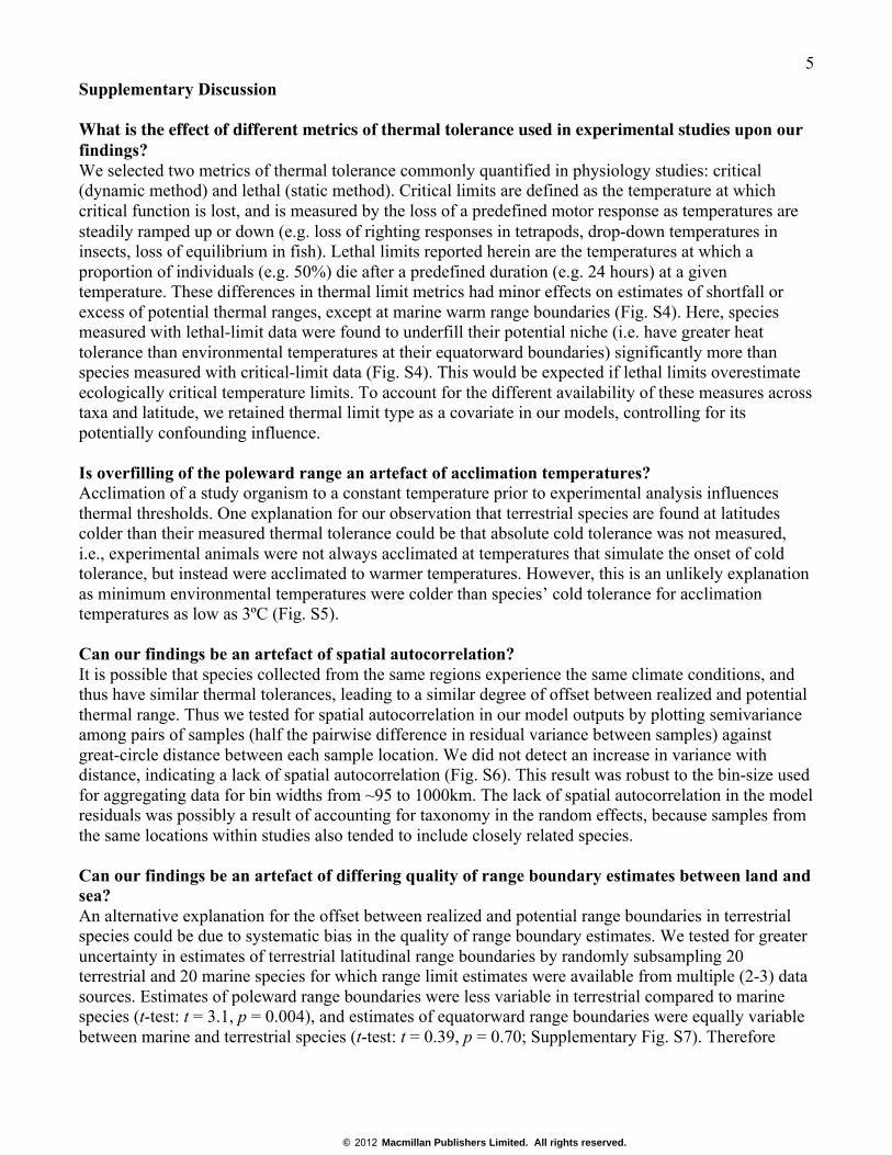
What is the effect of different metrics of thermal tolerance used in experimental studies upon our

findings?

We selected two metrics of thermal tolerance commonly quantified in physiology studies: critical

(dynamic method) and lethal (static method). Critical limits are defined as the temperature at which

critical function is lost, and is measured by the loss of a predefined motor response as temperatures are

steadily ramped up or down (e.g. loss of righting responses in tetrapods, drop-down temperatures in

insects, loss of equilibrium in fish). Lethal limits reported herein are the temperatures at which a

proportion of individuals (e.g. 50%) die after a predefined duration (e.g. 24 hours) at a given

temperature. These differences in thermal limit metrics had minor effects on estimates of shortfall or

excess of potential thermal ranges, except at marine warm range boundaries (Fig. S4). Here, species

measured with lethal-limit data were found to underfill their potential niche (i.e. have greater heat

tolerance than environmental temperatures at their equatorward boundaries) significantly more than

species measured with critical-limit data (Fig. S4). This would be expected if lethal limits overestimate

ecologically critical temperature limits. To account for the different availability of these measures across

taxa and latitude, we retained thermal limit type as a covariate in our models, controlling for its

potentially confounding influence.

Is overfilling of the poleward range an artefact of acclimation temperatures?

Acclimation of a study organism to a constant temperature prior to experimental analysis influences

thermal thresholds. One explanation for our observation that terrestrial species are found at latitudes

colder than their measured thermal tolerance could be that absolute cold tolerance was not measured,

i.e., experimental animals were not always acclimated at temperatures that simulate the onset of cold

tolerance, but instead were acclimated to warmer temperatures. However, this is an unlikely explanation

as minimum environmental temperatures were colder than species’ cold tolerance for acclimation

temperatures as low as 3ºC (Fig. S5).

Can our findings be an artefact of spatial autocorrelation?

It is possible that species collected from the same regions experience the same climate conditions, and

thus have similar thermal tolerances, leading to a similar degree of offset between realized and potential

thermal range. Thus we tested for spatial autocorrelation in our model outputs by plotting semivariance

among pairs of samples (half the pairwise difference in residual variance between samples) against

great-circle distance between each sample location. We did not detect an increase in variance with

distance, indicating a lack of spatial autocorrelation (Fig. S6). This result was robust to the bin-size used

for aggregating data for bin widths from ~95 to 1000km. The lack of spatial autocorrelation in the model

residuals was possibly a result of accounting for taxonomy in the random effects, because samples from

the same locations within studies also tended to include closely related species.

Can our findings be an artefact of differing quality of range boundary estimates between land and

sea?

An alternative explanation for the offset between realized and potential range boundaries in terrestrial

species could be due to systematic bias in the quality of range boundary estimates. We tested for greater

uncertainty in estimates of terrestrial latitudinal range boundaries by randomly subsampling 20

terrestrial and 20 marine species for which range limit estimates were available from multiple (2-3) data

sources. Estimates of poleward range boundaries were less variable in terrestrial compared to marine

species (t-test: t = 3.1, p = 0.004), and estimates of equatorward range boundaries were equally variable

between marine and terrestrial species (t-test: t = 0.39, p = 0.70; Supplementary Fig. S7). Therefore


6

uncertainty in range limit estimates is unlikely to explain the offset between equatorward range

boundaries and heat tolerance in terrestrial species.

Can our findings be an artefact of non-random sampling across longitudes?

Warm and cold temperatures vary across longitudes at any given latitude both on land and in the ocean.

Our calculations of potential latitudinal range boundaries used temperature metrics generalized for each

latitude, therefore any systematic bias in sampling species at warmer- or colder-than-average longitudes

may have affected overall patterns. Specifically, if terrestrial species were sampled at warmer-than-

average latitudes, this would generate the pattern we observed: equatorward range boundaries that are

truncated from the expectation as warm temperatures are warmer on average at the longitudes sampled,

and poleward range boundaries that extend further towards the poles than expected, as cold temperatures

are milder on average at the longitudes sampled. We tested for systematic bias in the longitudes sampled

in our dataset by calculating the difference between average temperatures experienced at species’

latitudinal range boundaries relative to the mean temperature for each latitude. For each species, we

calculated a ‘localized’ average warm temperature along a it’s equatorward latitudinal boundary, and a

‘localized’ average cold temperature along it’s poleward latitudinal boundary, including longitudes 5° W

and E of the longitude of specimen collection, and including only grid cells with suitable habitat (land or

ocean). We then calculated the difference between this local mean for the species and the grand mean

for the entire latitude. In some cases, the range of longitudes used for the local temperature mean was

extended by 5° units until suitable habitat (land or ocean) was sampled.

The residual difference between local means and grand means at a latitude were centred on zero for

terrestrial species at both poleward and equatorward range boundaries, and for marine species at

poleward range boundaries (Fig. S8a-c). The mean values were not significantly different than zero (t-

tests: terrestrial poleward range boundaries p=0.08, terrestrial equatorward range boundaries p=0.45,

marine poleward range boundaries p=0.95) (Fig. S8 a-c). The distribution of residual temperatures at

marine equatorward range boundaries was bimodal, with two peaks at ±~2°C, and the median residual

difference was lower than zero by 1.6°C in a Wilcoxin signed rank test (p=0.003). However, the peaks

in the distribution were attributable to multiple samples within studies, sampled from the same

longitude, and with the same equatorward range boundaries (at the equator). Because samples from the

same studies were usually taxonomically similar, we tested for a difference from zero in temperature

residuals when taxonomy was included as a random effect. With taxonomy included, none of the

modelled means differed from zero (terrestrial poleward range boundaries p=0.75, terrestrial

equatorward range boundaries p=0.71, marine poleward range boundaries p=0.82, marine equatorward

range boundaries p=0.18). Because taxonomy was also included in the full models, it is unlikely that

non-random sampling across longitudes affected the overall outcomes of underfilling and overfilling of

range boundaries found here (Fig. 1).

To what degree might species boundaries relate to precipitation?

It is clear that precipitation and water availability influence local diversityS20

and may influence the

distribution of organisms. Climate envelope models frequently include precipitation and/or a series of

derived precipitation metricseg.S21-23

. Ideally, we would test this question with experimental data on the

desiccation tolerance of species - analogous to the thermal tolerance data we’ve used here. Such data are

surprisingly hard to find. Instead we used available precipitation data across species’ geographic ranges

to test the expectation that precipitation-limited species would experience the lowest level of

precipitation at their equatorward range margin (Fig. S9). Species found between 20-40o degrees North,

and between 20-35o South, have equatorward range boundaries coincident with lowest level of

precipitation in their geographic range, and hence desiccation may limit their equatorward distribution.

A subset of species, mainly below 20° latitude, are unlikely to be precipitation-limited, because their


7

lowest level of precipitation is not encountered at their equatorward range boundary (shown by vertical

yellow bars in Fig. S9).

Are species ranges limited by rare extreme events?

Extreme heat may limit terrestrial species at their warm range boundaries in a manner not captured by

mean monthly climatologies. To explore this, we compared species’ heat tolerances to national record-

high temperatures available on a public web-server (see refS24

for citations). We found that the pattern of

extreme heat events recorded across latitude is greatest at mid-latitudes, and drops down at the equator,

in both hemispheres (Fig. S10). Because the temperatures of these events generally exceed the thermal

tolerances of species living there (Fig. S10), animals must survive heat events in cooler locations or

habitat refugia. However, this finding suggest that extreme heat events have the potential to limit

species’ range boundary locations, and greater sampling within species’ habitats and longitudes may

reveal closer correspondence between extreme heat events at species’ warm boundaries and the

extremes of their thermal tolerance.

What explains the difference between assemblage and single-species range shift results?

Both on land and in the ocean, observations of single-species poleward range shifts of leading range

boundaries (range expansions) have been more frequently recorded than poleward range shifts of trailing

range boundaries (range contractions). In the assemblage data sampling intensity of upper and lower

boundary shifts is standardized, by contrast it is not possible to standardize for sampling intensity in the

single-species data. Thus the excess of leading boundary shifts, and departure from a log-ratio of one

(Fig. 3b,c), may represent one or more of three biases: (1) a global bias towards sampling species at their

poleward compared to their equatorward latitudinal range limits, (2) a bias in detecting range expansions

compared to contractions (discussed in more detail below), or (3) a bias in attributing upper range limit

shifts to climate warmingS25

. Nevertheless, the level of asymmetry is greater among terrestrial single-

species studies, above and beyond the level of bias expected based on the marine single-species studies.

Is the asymmetry in terrestrial range boundary shifts due to differing climate velocities?

For the single-range limit analysis of range shifts, where paired observations are not available at a given

latitude, attributing the frequency of trailing boundary shifts to climate sensitivity relies on the

assumption that the velocity of climate change is similar across latitudes. This assumption appears to

hold in the latitudes sampled for marine and terrestrial systemsS26

.

Is the asymmetry in terrestrial range boundary shifts due to differing detectability?

The asymmetry of terrestrial responses to climate change could also be explained by lower detectability

of range boundary contractions compared to range boundary expansionsS27,28

. However, differential

detectability should have a greater effect in the oceans which receive far less research effortS29

. Where

elevational gradients are available, a downwards bias in the detection of trailing range boundary shifts

might also be expected because terrestrial species can move upwards on mountains to escape heat at

their equatorward limit. In such cases, the leading range boundary may not change, although the species

range has responded to increasing temperature, leading to a bias in the detection of the trailing boundary

responsesS27

. However, marine species can also move deeperS17

hence detection of equatorward

boundary shifts may be negatively biased in both systems depending on the extent of searching at

altitude and at depth. Marine fish assemblages in Table 1 each involved trawls to the 200 m depth and

beyond, indicating elevation/depth gain alone is not likely to account for the greater bias on land.


8

Fig. S1. Temperature extremes, thermal tolerance and latitudinal ranges of ectotherms in

Southern and Northern hemispheres.

Latitudinal ranges and thermal tolerance of marine (a,b) and terrestrial (c,d) species, with latitudinal

range on x-axis, and thermal tolerance on y-axis. Latitudinal ranges and thermal limits are shown in

relation to mean temperature of warmest month (curved lines in a, c) and coldest month (b, c). Error

around environmental temperature curves indicate standard deviation of values across longitudes at each

latitude (colour-shaded regions). Dashed grey lines indicate the extent to which some species underfill

their potential thermal ranges. Negative latitudes denote the Southern hemisphere. Colours of horizontal

lines denote the thermal limit metric used for each species (lethal vs. critical limits).


9

Fig. S2. Overfilling and underfilling of range boundaries with species’ mid-latitude. Extent to

which terrestrial and marine species overfill (positive values) or underfill (negative values) their

potential latitudinal range based on temperature tolerance as a function of absolute mid-latitude of

species distribution. Shortfall or excess are in units of degrees latitude, calculated as the difference

between the potential and realized latitudinal range boundary. Grey shading shows areas of the plot

where data cannot fall because potential warm range boundaries are constrained by the equator and

potential cold range boundaries are constrained by the poles (90° latitude). Species for which range

limits were estimated using critical thermal limits (circles) and lethal thermal limits (diamonds) are both

shown. Adjacent bean plots shows the density distribution of the data and horizontal bars show the

median value. Black line in (b) denotes significant best-fit line from the model-averaged mixed-effects

models.


10

Fig. S3.

Relationship between latitudinal range boundary and thermal tolerance limit.

a,b marine species. c,d terrestrial species. a,c Poleward range boundary and cold tolerance limit, b,d

equatorward range boundary and heat tolerance limit. Triangles represent intertidal marine species,

which were not included in the potential/realized range boundary analyses. Lines represent significant

model-averaged coefficients (see Tables S2-S3) when intertidal data are included (solid) or when

intertidal data are excluded (dashed grey).


11

Fig. S4.

Effect of thermal tolerance metrics on degree of offset

Beanplots show the relative density of species that overfill (positive values) or underfill (negative

values) their potential latitudinal range according to the critical (lefthandside of bean) or lethal (RHS of

bean) thermal limit metric used. Units of shortfall or excess are in degrees latitude, calculated as the

difference between the potential and realized latitudinal range boundary based on thermal physiological

limits. Width of beanplot denotes relative density, and large horizontal bar denotes median value. Short

horizontal bars show individual data in each category.


12

Fig. S5. Effect of acclimation on degree of poleward range boundary offset in terrestrial species.

Extent of overfilling (positive values) and underfilling (negative values) of poleward range boundaries

in terrestrial species against absolute latitude of specimen collection. Colours denote the acclimation

temperature used for each thermal limit measurement. Data shown are a subset of terrestrial species for

which acclimation temperatures were available.


13

Fig. S6. Testing for spatial autocorrelation in model outputs.

Average pairwise difference in model residual variance (semivariance), plotted against great-circle

distance between sample locations. Data shown are binned by 96 km (terrestrial) and 92 km (marine)

increments (200 bins between minimum and maximum distance). No increase in variance with distance

indicates a lack of spatial autocorrelation.


14

Fig. S7. Homogeneity in quality of range limit estimates.

Standard deviation, in degrees latitude, of (a) poleward range boundary estimates and (b) equatorward

range boundary estimates, for species in which range limits could be obtained from multiple data

providers (2-3 providers per species). Whisker plots denote the median, upper and lower quartiles, and

extremes values.


15

Fig. S8. Potential for longitudinal temperature bias when using local longitudinal means as a

proxy for local climate.

Difference between localized mean temperatures at longitudes near specimen collection (±5° longitude

from collection point, at poleward or equatorward range boundaries), and the grand mean across the

entire latitudinal band, in terrestrial (a,b) and marine (c,d) taxa. Positive differences, or ‘residuals’,

represent species located at longitudes with warmer-than-average temperatures at their poleward (a,c) or

equartorward (b,d) range boundaries. Dashed lines denote mean residual value.


16

Fig. S9. Latitudinal ranges and precipitation.

Terrestrial species’ range boundaries (green horizontal bars) are shown relative to the mean precipitation

across latitude (black line) in the northern (N) and southern (S) hemispheres. The height of each species

along the y-axis indicates the minimum precipitation experienced throughout its range. Points indicate

equatorward range boundaries. Yellow vertical bars show where the minimum latitudinal range

boundary does not coincide with its minimum experienced precipitation.


17

Fig. S10. Extreme weather events, thermal tolerance, and latitude on land.

Record-high temperatures for various countries within the last century and their locations across latitude

(yellow points). Black line shows the maximum temperature per 5 degrees of latitude. Green horizontal

lines indicate latitudinal ranges of terrestrial species along the x-axis, and their maximum thermal

tolerance on the y-axis. Most species have heat tolerances below the most extreme temperatures

potentially experienced in their range within the last century, hence extreme heat events may be a better

predictor of species’ ranges than mean temperature of the warmest month.


18

Fig. S11. Schematic representation of assemblage-level range shifts.

Assemblage-level studies are defined as those that analysed distributional responses of multiple species

within a fixed region. The portion of the latitudinal range captured in the sampling area differed among

species. We identified species where either the equatorward (a) or poleward (b), or both range limits (c)

were examined for a given species. Cosmopolitan species found throughout the latitudinal scope of the

study (d) were excluded. Decreases in the abundance of species distributed at higher latitudes than the

study region (a) were considered equatorward boundary range contractions. Likewise, increases in

abundance of species historically distributed towards the equator (b) were considered poleward

boundary range expansions.


19

Table S1. Parameter estimates for linear mixed effects models testing degree of overfilling and

underfilling of potential range boundaries. If multiple models fell within the 95% confidence set (see

Table S3), model-averaged parameter estimates and unconditional errors based on Akaike Information

Criterion (AIC) are shown. If, however, only one model fell within the 95% confidence set, the

parameter estimates and p-values from the top model are shown. Effect types are intercepts (unshaded)

and slopes (shaded). Helmert contrast coefficients are presented for each model parameter, so

coefficients represent the overall intercept (Intercept), overall slope (Mid-latitude, Elevation), and the

increase/decrease from the overall intercept or slope for different levels of categorical variables. Levels

of categorical variables are shown in brackets, in order, such that the contrast coefficient shows the

effect of the first level, and the negative effect of the second level. § symbol indicates contrast

coefficients with 95% confidence intervals greater than 0, or p-values below 0.05. Inclusion of

taxonomic random effects was determined based on AIC comparisons prior to model averaging, model

improvement when taxonomy is included is indicated by delta AIC (dAIC) proceeding model. If

taxonomy did not provide model improvement, it was not included.

(a) Terrestrial warm boundaries

Degree of offset = mid-latitude + elevation + limit type, random=C/O/F/Genus

dAIC without taxonomic inclusion: 71.7

95% confidence set only included a single model, therefore non-averaged results shown

Fixed-effects Contrast coefficient Standard error p-value

Intercept 2.02 4.65 0.666

Mid-latitude -0.406 0.091 <0.0001 §

(b) Terrestrial cold boundaries

Degree of offset = mid.latitude + elevation + limit type, random=C/O/F/Genus




Intercept -6.19 1.82 0.0013 §

Mid-latitude 0.724 0.047 <0.0001 §

Elevation -0.0053 0.0012 <0.0001 §

Limit type (lethal, critical) -6.64 1.57 0.0001 §

(c) Marine warm boundaries

Degree of offset = mid.latitude +limit type, random=O/F/Genus


Fixed-effects Contrast coefficient Unconditional

Standard error

Lower 95%

limit

Upper 95%

limit

Intercept -4.90 5.76 -17.0 7.2

Mid-latitude -0.0987 0.235 -0.603 0.406

Limit type (lethal, critical) -6.55 2.35 -12.0 -1.10 §

(d) Marine cold boundaries

Degree of offset = mid.latitude +limit type

dAIC with taxonomic inclusion: -1.81, therefore not included as random effect



Intercept -2.65 1.38 0.065

Limit type (lethal, critical) -5.08 1.38 0.0009 §


20

Table S2. Parameter estimates for linear mixed effects models testing position of range boundaries

relative to thermal tolerance. If multiple models fell within the 95% confidence set (see Table S3),

model-averaged parameter estimates and unconditional errors based on Akaike Information Criterion

(AIC) are shown. If, however, only one model fell within the 95% confidence set, the parameter

estimates and p-values from the top model are shown. Effect types are intercepts (unshaded) and slopes

(shaded). Helmert contrast coefficients are presented for each model parameter, so coefficients represent

the overall intercept (Intercept), overall slope (Tmin, Tmax), and the increase/decrease from the overall

intercept or slope for different levels of categorical variables. Levels of categorical variables are shown

in brackets, in order, such that the contrast coefficient shows the effect of the first level, and the negative

effect of the second level. § symbol indicates contrast coefficients with 95% confidence intervals greater

than 0 or with p-values less than 0.05. Random effects and error structures included in the full model

were determined based on AIC comparisons prior to model averaging.

(a) Poleward range boundary

Poleward boundary ~ tmin*habitat+limit type, varExp(form=~ tmin), random=C/O/F/G

Fixed-effects

Contrast

coefficient

Standard

error

Lower 95%

interval

Upper 95%

interval

Intercept 47.3 1.7 44.0 50.6 §

Tmin -1.57 0.14 -1.86 -1.28 §

Habitat (terrestrial/marine) 5.74 1.57 -1.91 9.58 §

Tmin:Habitat (terrestrial/marine ) -0.08 0.15 -0.37 0.21

Limit type (critical/lethal) 2.82 1.39 -3.78 1.67

(b) Equatorward range boundary

Equatorward boundary ~ tmax*habitat+ limit type, random=C/O/F/G


Fixed-effects

Contrast

coefficient

Standard

error

p-value

Intercept 45.1 8.62 0.000 §

Tmax -0.55 0.21 0.012 §

Habitat (terrestrial/marine ) -31.1 8.57 0.011 §

Tmax:Habitat (terrestrial/marine ) 0.85 0.21 0.0002 §


21

Table S3. 95% confidence sets of models based on AICc (Akaike's information criterion corrected for

finite sample sizes). For four of six models, the 95% confidence set only included one model.

Model Model structure dAICc weight

Terrestrial warm

boundary offset

Mid.latitude, random=C/O/F/G 0 0.759

Terrestrial cold

boundary offset

Mid.latitude + Elevation + Limit type, random=C/O/F/G 0 0.571

Marine warm

boundary offset

Limit type, random=C/O/F/G 0 0.632

Mid.latitude + Limit type, random=C/O/F/G 2.90 0.148

Mid.latitude, random=C/O/F/G 2.98 0.142

1, random=C/O/F/G 4.18 0.078

Marine cold

boundary offset

Limit type 0 0.726

Poleward

boundary

Tmin+Habitat, random= P/C/O/F/G 0 0.416

Tmin+Habitat+limit type, random=P/C/O/F/G 1.155 0.234

Tmin+Habitat+(Tmin:Habitat), random=P/C/O/F/G 1.44 0.203

Tmin+Habitat+(Tmin:Habitat)+Limit type,

random=P/C/O/F/G

2.345 0.129

Equatorward

boundary

Tmax+Habitat+(Tmax:Habitat), random=P/C/O/F/G 0 0.62


22

Table S4. Summary of single range-boundary range shift studies. Table includes studies reporting

poleward shifts at poleward or equatorward range boundaries, or shifts in abundance of northerly or

southerly species, correlated with recent changes in temperature, in marine and terrestrial ectotherms.

Asterisk (*) denotes species limits not included in analyses and Fig. 3, because they are already counted

once in assemblage-scale data, or elsewhere within table.

Location Study

Latitude Animal type

Species name or

proportion of

species group

shifted

Shift

direction

Poleward/

equatorward

limit

Reference & Data Details

Marine - shifts in upper/lower latitude limit

Gulf of

Mexico, USA 25ºN

Cnidaria

(coral) Acropora palmate poleward

poleward

limit

Ref.S30

; distribution literature is

reviewed

Acropora cercisornis poleward

poleward

limit

“

California

Gulf, USA 30° N

Mollusca

(abalone)

Haliotis walallensis poleward

equatorward

limit

Ref.S31

; distribution surveys at two time

periods (1979 vs. 2005)

California

Gulf, USA 34ºN

Mollusca

(snail) Kelletia kelletii poleward

poleward

limit

Ref.S32


reviewed

Japan 30-35°N Cnidaria

(coral)

Acropora hyacinthus poleward

poleward

limit Ref.

S33; 1931-2010 National records

Acropora muricata poleward

poleward

limit

Acropora solitaryensis poleward

poleward

limit

Pavona decussata poleward poleward

limit

Southern

Atlantic, USA 35ºN

Mollusca

(mussel) Mytilus edulis L.* poleward

equatorward

limit

Ref.S34

; distribution survey data

combined with experimental transplant

study

California

Gulf, USA 41ºN Fish

Entelurus aequoreus* poleward

poleward

limit Ref.

S35; fishing survey data

Tasman Sea,

Australia 38ºS

Echinoderm

ata (urchin)

Centrosetphanus rodgersii poleward

poleward

limit

Ref.S36


reviewed

Sea of Japan,

Japan 42ºN

Echinoderm

ata (urchin)

Hemicentrotus pulcherrimus poleward

poleward

limit

Ref.S37

; annual distribution surveys

(1980-2005)

Tasman Sea,

Australia 40-43ºS Fish 30 species poleward

poleward

limits

Ref.S38

; RefS39

; historical fisheries

records vs. compiled information from

scientists, scuba divers and fishers;

temperature increase due to ocean

circulation changes. Species from both

studies cross-referenced to avoid

double-counting.

Bay of

Biscay,

France

43ºN Arthropoda

(barnacle)

Semibalanus balanoides poleward

equatorward

limit

Ref.S40

; distribution surveys at several

time periods (historical surveys vs.

2006)

45ºN

Annelida

(polychaete)

Diopatera neapolitana poleward

poleward

limit “


23

Bay of

Biscay,

France

44ºN Annelida

(polychaete) Diopatra sp. A poleward

poleward

limit

Ref.S41

; distribution surveys at two time

periods (late 1800s vs. 2006)

Irish Sea,

Ireland 45ºN

Porifora

(sponge)

Hexadella racovitzai poleward

poleward

limit

Ref.S42


reviewed

Bering Sea,

USA 50ºN

Arthropoda

(euphausiid)

Thysanoessa inspinata poleward

poleward

limit

Ref.S43

; distribution surveys (historical

data vs. 1997-2002)

Wadden Sea 53ºN Mollusca

(bivalve) Macoma balthica poleward

equatorward

limit

Ref.S44

; annual distribution surveys

(1970-2007); Jansen et al. 2007;

experimental transplant study

Irish Sea, UK 54ºN Mollusca

(snail)

Tectura testudinalis poleward

poleward

limit

Ref.S45

; cited by author as unpublished

data

Bering Sea,

USA 57ºN

Arthropoda

(crab)

Chionoecetes opilio poleward

equatorward

limit Ref.

S46; fishing survey data (1975-2001)

Arctic Ocean,

Norway 61ºN Fish

Entelurus aequoreus* poleward

poleward

limit

Ref.S47

; survey data (historical

distribution vs. 2006)

Arctic Ocean,

Norway 72ºN

Mollusca

(mussel) Mytilus edulis L.* poleward

poleward

limit

Ref.S48


distribution vs. 2004)

Marine - shifts in abundance

Bansho Cape,

Japan ~33ºN Molluscs

not available (>1

species) increase poleward

limits

Ref.S49

; abundance surveys (1985 -

1994); winter temperature and ocean

current changes implicated

Gulf of

California,

USA

35ºN Fish Oncorhynchus mykiss decrease

equatorward

limit

Ref.S50

; local extirpation events at the

lower range limit; habitat modification

and temperature implicated

Gulf of

California,

USA

35ºN Mollusc

(abalone)

Haliotis kamtschatkana decrease

equatorward

limit

Ref.S31

; presence data from two time

periods (1959 vs. 2005)

Mid-Atlantic

Coast, USA 37ºN

Mollusc

(clam)

Spisula solidissima decrease

equatorward

limit

Ref.S51

; survey data at the lower range

limit (1994, 1997, 1999 & 2002)

Gulf of

Maine, USA 40ºN

Echinoderm

(sea star) Asteria vulgaris decrease

equatorward

limit Ref.

S52; survey data (1976 vs. 1996)

Asteria forbesi increase

poleward

limit “

Portugal and

UK 40ºN

Arthropod

(barnacle)

Solidobalanus fallax increase

poleward

limit

Ref.S53

; compiled records from various

sources (1995-2004)

Bay of

Biscay,

France

44ºN Fish Capros aper* increase poleward

limit

Ref.S54

; abundance per haul data

(various years from 1973-2003)

Tasmania 43°S Zooplankton

Calanus australis Centropages australiensis Neocalanus tonsus

decrease equatorward

limit

Ref.S39

; 1970-73 vs. 2000-09. Species

with ≥2 years abundance shifts counted.

Tasmania 43°S Zooplankton

Acartia danae Corycaeus spp. Pleuromamma gracilis Sapphirina spp.

increase poleward

limit

Ref.S39

; 1970-73 vs. 2000-09. Species

with ≥2 years abundance shifts counted.

English

Channel, UK ~49ºN Chaetognath Sagitta elegans decrease

equatorward

limit

Ref.S14

; data represent case species in

manuscript

Sagitta setosa increase

poleward

limit

“

Arthropod

(copepod & Eucalanus sp. decrease

equatorward

limit

“

barnacle) Calanus sp. increase

poleward

limit

“


24

Chthmalus sp. increase

poleward

limit

“

Monodontu lineate increase

poleward

limit

“

Aglantha digitalis decrease

equatorward

limit

“

Fish Sardina pilchardus* increase

poleward

limit

“

Clupea herengis* decrease equatorward

limit

“

UK ~54ºN Mollusc

(snail) Osilinus lineatus increase

poleward

limit

Ref.S55

; survey data (1950s vs. 2001-

2003)

~54ºN

Gibbula umbilicalis increase

poleward

limit “

North Sea,

UK 54ºN

Arthropod

(cladoceran) Penilia avirostris increase

poleward

limit

Ref.S56

; monthly Continuous Plankton

Recorder survey data (various years

from 1990-2004)

Ireland 51-55ºN Invertebrate Balanus crenatus decrease equatorward

limit

Ref.S57

; qualitative abundance surveys

(1958 vs. 2003); temperature and

operator error implicated

Littorina littorea decrease equatorward

limit “

North Sea,

Norway 58ºN

Arthropod

(copepod)

Calanus finmarchicus decrease

equatorward

limit

Ref.S58

; ICES survey data (1985-1995);

change in C. harengus attributed to low

prey abundance and temperature

Fish Clupea harengus* increase poleward

limit “

Bering Sea,

USA 59ºN Fish

Gadus macrocephalus increase

poleward

limit Ref.

S46; survey data (1981–2000)

Terrestrial - shifts in upper/lower latitude limit

UK 50-60ºN

Amphibian,

Reptile,

Fish,

Arthropod

(various

taxa)

195 species poleward poleward

limits

Ref.S59

; survey data for

presence/absence in 10-km grid squares

(two recording periods of ~11 years,

spaced by 14 years between 1965 and

2005); to discount endotherms and

species sampled elsewhere (butterflies

and dragonflies), maximum number of

mammal (9), bird (22), butterfly (29)

and dragonfly (20) range shifts were

removed from the total number range

shifts reported (275).

Florida, USA ~22ºN Arthropod

(butterfly)

Coryphaeschna adnexa poleward

poleward

limit

Ref.S60

; survey data (1889-1991 vs.

1989)

Chrysobasis lucifer poleward

poleward

limit “

Erythemis plebeja poleward poleward

limit “

Microathyria aequalis poleward

poleward

limit “

Microathyria didyma poleward

poleward

limit “

Nehalennia minuta poleward

poleward

limit “


25

Central Japan 34ºN Arthropod

(stick bug) Nezara viridula poleward

poleward

limit

Ref.S61

; survey data (1961 to 1962 vs.

1999-2007)

Africa,

Mediterranea

n Region

35ºN Arthropod

(butterfly)

Danaus chrysippus poleward

poleward

limit

Ref.S62


reviewed

Southeastern

USA 39ºN

Arthropod

(beetle)

Dendroctonus frontalis poleward

poleward

limit Ref.

S63; survey data (1987-2004)

Mediterranea

n Region 40ºN

Arthropod

(dragonfly)

Trithemis annulata poleward

poleward

limit Ref.


Washington,

USA 45ºN

Arthropod

(butterfly)

Atalopedes campestris poleward

poleward

limit

Ref.S65


reviewed

Germany ~46ºN Arthropod

(butterfly)

Crocothemis erythraea poleward

poleward

limit

Ref.S66


reviewed (1970 until present)

Northern Italy 47ºN Arthropod

(moth)

Thaumetopoea pityocampa poleward

poleward

limit Ref.


UK 50ºN Arthropod

(butterfly) Pyronia tithonus* poleward

poleward

limit Ref.

S68; distribution data is reviewed

UK 54ºN Arthropod

(butterfly) Aricia artaxerxes poleward

equatorward

limit

Ref.S25

; survey data (1970 to 1982

vs.1995-1999)

Erebia aethiops poleward

equatorward

limit

“

UK 57ºN Arthropod

(butterfly) Pararge aegeria* poleward

poleward

limit

Ref.S69


distribution vs. 1940-1989 and 1990-

1997)

Sweden 64ºN Arthropod

(tick) Ixodes ricinus poleward

poleward

limit

Ref.S70

; data based on questionnaires

distributed to 1000 participants (early

1980s and mid-1990s)

Finland 60-69ºN Arthropod

(butterfly) 14 species* poleward

poleward

limits

Ref.S71

; surveys for presence/absence in

10-km grid squares (1992-1996 vs.

2000-2004); species shifting < 30 km

were excluded; 13 species also sampled

in assemblage-scale data were excluded

Northern

Fennoscandia 70ºN

Arthropod

(moth)

Operophtera brumata poleward

poleward

limit

Ref.S72

; survey data (1862-1968 vs.

1969-2001)

Northern

Fennoscandia 70°N

Arthropod

(moth)

Epirrita autumnata poleward

poleward

limit Ref.

S73

Europe 69°N Arthropod

(tick) Ixodes rinicus poleward

poleward

limit Ref.

S74;survey data (1943, 1983, 2009)

Norway 72ºN Arthropod

(moth) Plutella xylostella poleward

poleward

limit

Ref.S75

; warm air currents transported

moths to the arctic islands in 2000

Terrestrial - shifts in abundance

Australia 20ºS Reptile

(lizard)

Liopholis kinetorei decrease

equatorward

limit

Ref.S19

; survey data (see manuscript for

details); habitat modification and

climate change implicated

Mexico 30ºN Arthropod

(butterfly)

Euphydryas editha decrease

equatorward

limit

Ref.S76

; survey data (historical data

vs.1992-1996)

Czech

Republic ~49ºN

Arthropod

(cricket)

Phaneroptera nana increase

poleward

limit

Ref.S77

; historical data and surveys

(1995-2007)

Phaneroptera falcata increase

poleward

limit

“


26


(cricket)

Conocephalus fuscus increase

poleward

limit Ref.

S78; as cited in Ref.

S79


(cricket)

Metrioptera roeselii increase

poleward

limit Ref.

S79; survey data (1990-2004)

UK 59ºN Arthropod

(fly) Coelopa pilipes increase

poleward

limit

Ref.S80

; survey data (historical data vs.

2004-2005)

Europe 40ºN Arthropod

(butterfly) Colotis evagore increase

poleward

limit

Ref.S81

; review paper presented

compiled data on range extension of

insects in Europe from the late 1800s to

present

41ºN Colias erate* increase

poleward

limit “

50ºN Apamea Illyria increase

poleward

limit

“

50ºN

Araschnia levana* increase

poleward

limit

“

50ºN

Autographa buraetica increase

poleward

limit

“

50ºN

Autographa mandarina increase

poleward

limit

“

50ºN Brenthis ino* increase

poleward

limit

“

50ºN

Chlorantha hyperici increase

poleward

limit

“

50ºN Colias erate increase

poleward

limit

“

50ºN

Cucullia artemisiae increase

poleward

limit

“

50ºN

Cucullia fraudatrix increase

poleward

limit

“

50ºN Erebia ligea* increase

poleward

limit

“

50ºN Libythea celtis increase

poleward

limit

“

50ºN

Lithophane leautieri increase

poleward

limit

“

50ºN Lycaena tityrus increase

poleward

limit

“

50ºN

Macdunnoughia confusa increase

poleward

limit

“

50ºN Opigena polygona increase

poleward

limit

“

50ºN Pararge aegeria* increase

poleward

limit

“

50ºN

Polygonia c-album increase

poleward

limit

“

50ºN

Staurophora celsia increase

poleward

limit

“

46ºN

Polistes dominulus increase

poleward

limit

“

49ºN Xylocopa violacea increase

poleward

limit

“

50ºN

Dolichovespula media increase

poleward

limit

“

50ºN

Dolichovespula saxonia increase

poleward

limit

“

52ºN

Meconema thalassinum increase

poleward

limit

“


27

52ºN (bee, wasp)

Platycleis albopunctata increase

poleward

limit

“

52ºN

Tettigonia viridissima increase

poleward

limit

“

52ºN

Conocephalus dorsalis increase

poleward

limit

“

52ºN

Stenobothrus lineatus increase

poleward

limit

“

52ºN Omocestus rufipes increase

poleward

limit

“

52ºN Tetrix subulata increase

poleward

limit

“

54ºN (grasshopper

, cricket)

Chorthippus albomarginatus increase

poleward

limit

“


28

Table S5. Low sensitivity of range shift results to inclusion criteria.

Chi-square tests between the frequency of poleward range shifts at equatorward range boundary vs.

poleward range boundaries, given various inclusion criteria for range shifts. Results are robust to

different inclusion criteria: there is an excess of poleward range boundary shifts in terrestrial species,

indicated by negative log ratios, but no access of poleward range boundary shifts in marine species,

indicated by log ratios close to zero. See methods for details of inclusion criteria.

Data inclusion

criterion

habitat

Equa.

boundary

shifts

Poleward

boundary

shifts

Equa.

Boundaries

sampled

Poleward

boundaries

sampled

log ratio of

poleward:

equatorward

range shift

frequencies

χ2 P-value

shifts <60km

considered stable

marine 37 73 49 101 0.019 0.001 0.976

terrestrial 56 76 14 44 0.36 5.032 0.025*

shifts <30km

considered stable†

marine 35 73 49 101 -0.005 0.008 0.928

terrestrial 52 76 12 44 0.399 5.511 0.019*

shifts <20km

considered stable

marine 37 73 49 101 0.019 0.001 0.976

terrestrial 52 76 12 44 0.399 5.511 0.019*

all reported shifts

(>0km)

considered

significant

marine 37 73 49 101 0.019 0.001 0.98

terrestrial 51 76 12 44 0.391 5.238 0.022*

harvested stocks

with contractions

at both limits not

excluded

marine 37 74 47 101 0.032 0.018 0.893

terrestrial 52 76 12 44 0.399 5.511 0.019*

† criterion used in main results


29

Supplementary References

S1. Sunday, J.M., Bates, A.E., and Dulvy, N.K., Global analysis of thermal tolerance and latitude in

ectotherms. Proc. R. Soc. Lond., Ser. B: Biol. Sci. 278, 1823-1830 (2011).

S2. Global Biodiversity Information Facility. Data for individual species accessed through GBIF

Data Portal, http://data.gbif.org, between 2008-03-01 and 2009-02-10.

S3. Hijmans, R.J. et al., Very high resolution interpolated climate surfaces for global land areas.

International Journal of Climatology 25, 1965-1978 (2005).

S4. Tyberghein, L. et al., Bio-ORACLE: a global environmental dataset for marine species

distribution modeling. Global Ecol. Biogeogr. 21, 272-281 (2011).

S5. Pinheiro, J. et al., nlme: Linear and Nonlinear Mixed Effects Models (R package version 3.1-96,

2009).

S6. Bartoń, K., MuMIn: Multi-model inference. R package version 1.5.2. 2011).

S7. R Development Core Team, R: A Language and Environment for Statistical Computing (Vienna,

Austria, 2009).

S8. Parmesan, C. et al., Poleward shifts in geographical ranges of butterfly species associated with

regional warming. Nature 399, 579-583 (1999).

S9. Sagarin, R.D., Barry, J.P., Gilman, S.E., and Baxter, C.H., Climate-related change in an intertidal

community over short and long time scales. Ecol. Monogr. 69, 465-490 (1999).

S10. Nye, J.A., Link, J.S., Hare, J.A., and Overholtz, W.J., Changing spatial distribution of fish stocks

in relation to climate and population size on the Northeast United States continental shelf. Mar. Ecol. Prog. Ser. 393, 111-129 (2009).

S11. Fodrie, F.J. et al., Climate-related, decadal-scale assemblage changes of seagrass-associated

fishes in the northern Gulf of Mexico. Global Change Biol. 16, 48-59 (2010).

S12. Reichert, K. and Buchholz, F., Changes in the macrozoobenthos of the intertidal zone at

Helgoland (German Bight, North Sea): a survey of 1984 repeated in 2002. Helgol. Mar. Res. 60,

213-223 (2006).

S13. Flenner, I. and Sahlen, G., Dragonfly community re-organisation in boreal forest lakes: rapid

species turnover driven by climate change? Insect Conservation and Diversity 1, 169-179 (2008).

S14. Southward, A.J., Hawkins, S.J., and Burrows, M.T., 70 years observations of changes in the

distribution and abundance of zooplankton and intertidal organisms in the western English

Channel in relation to rising sea temperature. J. Therm. Biol. 20, 127-155 (1995).

S15. Barry, J.P., Baxter, C.H., Sagarin, R.D., and Gilman, S.E., Climate-Related, Long-Term Faunal

Changes in a California Rocky Intertidal Community. Science 267, 672-675 (1995).

S16. Perry, A.L., Low, P.J., Ellis, J.R., and Reynolds, J.D., Climate change and distribution shifts in

marine fishes. Science 308, 1912-1915 (2005).

S17. Dulvy, N.K. et al., Climate change and deepening of the North Sea fish assemblage: a biotic

indicator of warming seas. J. Appl. Ecol. 45, 1029-1039 (2008).

S18. Poulard, J.-C. and Blanchard, F., The impact of climate change on the fish community structure

of the eastern continental shelf of the Bay of Biscay. ICES Journal of Marine Science: Journal du Conseil 62, 1436-1443 (2005).

S19. Sinervo, B., Fausto Méndez-de-la-Cruz, Donald B. Miles , Benoit Heulin, et al., Erosion of

Lizard Diversity by Climate Change and Altered Thermal Niches. Science 328, 894-899 (2010).

S20. Currie, D.J., Energy and large-scale patterns of animal-species and plant-species richness. Am. Nat. 137, 27-49 (1991).

S21. Suarez-Seoane, S., Osborne, P.E., and Rosema, A., Can climate data from METEOSAT improve

wildlife distribution models? Ecography 27, 629-636 (2004).

S22. Thuiller, W. et al., Climate change threats to plant diversity in Europe. Proceedings of the National Academy of Sciences of the United States of America 102, 8245-8250 (2005).


30

S23. Lobo, J.M., Verdu, J.R., and Numa, C., Environmental and geographical factors affecting the

Iberian distribution of flightless Jekelius species (Coleoptera : Geotrupidae). Divers. Distrib. 12,

179-188 (2006).

S24. List of weather records. In Wikipedia, The Free Encyclopedia. Retrieved November 30, 2011,

http://en.wikipedia.org/wiki/List_of_weather_records.

S25. Franco, A.M.A. et al., Impacts of climate warming and habitat loss on extinctions at species'

low-latitude range boundaries. Global Change Biol. 12, 1545-1553 (2006).

S26. Burrows, M.T. et al., The Pace of Shifting Climate in Marine and Terrestrial Ecosystems.

Science 334, 652-655 (2011).

S27. Thomas, C.D., Franco, A.M.A., and Hill, J.K., Range retractions and extinction in the face of

climate warming. Trends Ecol. Evol. 21, 415-416 (2006).

S28. Hampe, A. and Petit, R.J., Conserving biodiversity under climate change: the rear edge matters.

Ecol. Lett. 8, 461-467 (2005).

S29. Richardson, A.J. and Poloczanska, E.S., Ocean Science: Under-Resourced, Under Threat.

Science 320, 1294-1295 (2008).

S30. Precht, W.F. and Aronson, R.B., Climate flickers and range shifts of reef corals. Front. Ecol. Environ. 2, 307-314 (2004).

S31. Rogers-Bennett, L., Is climate change contributing to range reductions and localized extinctions

in northern (Haliotis kamtschatkana) and flat (Haliotis walallensis) abalones? Bull. Mar. Sci. 81,

283-296 (2007).

S32. Zacherl, D., Gaines, S.D., and Lonhart, S.I., The limits to biogeographical distributions: insights

from the northward range extension of the marine snail, Kelletia kelletii (Forbes, 1852). J. Biogeogr. 30, 913-924 (2003).

S33. Yamano, H., Sugihara, K., and Nomura, K., Rapid poleward range expansion of tropical reef

corals in response to rising sea surface temperatures. Geophys. Res. Lett. 38, L04601 (2011).

S34. Jones, S.J., Lima, F.P., and Wethey, D.S., Rising environmental temperatures and biogeography:

poleward range contraction of the blue mussel, Mytilus edulis L., in the western Atlantic. J. Biogeogr., 1-17 (2010).

S35. Sturm, E.A. and Horn, M.H., Increase in occurrence and abundance of zebraperch (Hermosilla azurea) in the Southern California Bight in recent decades. Bulletin Southern California Academy of Sciences 100, 170-174 (2001).

S36. Ling, S.D., Range expansion of a habitat-modifying species leads to loss of taxonomic diversity:

a new and impoverished reef state. Oecologia 156, 883-894 (2008).

S37. Agatsuma, Y. and Hoshikawa, H., Northward extension of geographic range of the sea urchin

Hemicentrotus pulcherrimus in Hokkaido, Japan. J. Shellfish Res. 26, 629-635 (2007).

S38. Last, P.R. et al., Long-term shifts in abundance and distribution of a temperate fish fauna: a

response to climate change and fishing practices. Global Ecol. Biogeogr. 20, 58-72 (2010).

S39. Johnson, C.R. et al., Climate change cascades: Shifts in oceanography, species' ranges and

subtidal marine community dynamics in eastern Tasmania. J. Exp. Mar. Biol. Ecol. 400, 17-32

(2011).

S40. Wethey, D.S. and Woodin, S.A., Ecological hindcasting of biogeographic responses to climate

change in the European intertidal zone. Hydrobiologia 606, 139-151 (2008).

S41. Berke, S.K. et al., Range shifts and species diversity in marine ecosystem engineers: patterns and

predictions for European sedimentary habitats. Global Ecol. Biogeogr. 19, 223-232 (2010).

S42. Picton, B.E. and Goodwin, C.E., Sponge biodiversity of Rathlin Island, Northern Ireland. J. Mar. Biol. Assoc. U.K. 87, 1441-1458 (2007).

S43. Lindley, J.A., Batten, S.D., Coyle, K.O., and Pinchuk, A.I., Regular occurrence of Thysanoessa

inspinata (Crustacea: Euphausiacea) in the Gulf of Alaska. J. Mar. Biol. Assoc. U.K. 84, 1033-

1037 (2004).


31

S44. Beukema, J.J., Dekker, R., and Jansen, J.M., Some like it cold: populations of the tellinid bivalve

Macoma balthica (L.) suffer in various ways from a warming climate. Marine Ecology-Progress Series 384, 135-145 (2009).

S45. Hawkins, S.J. et al., Complex interactions in a rapidly changing world: responses of rocky shore

communities to recent climate change. Clim. Res. 37, 123-133 (2008).

S46. Orensanz, J. et al., Contraction of the geographic range of distribution of snow crab

(Chionoecetes opilio) in the eastern Bering Sea: An environmental ratchet? California Cooperative Oceanic Fisheries Investigations Reports 45, 65-79 (2004).

S47. Fleischer, D., Schaber, M., and Piepenburg, D., Atlantic snake pipefish (Entelurus aequoreus)

extends its northward distribution range to Svalbard (Arctic Ocean). Polar Biol. 30, 1359-1362

(2007).

S48. Berge, J., Johnsen, G., Nilsen, F., Gulliksen, B., Slagstad, D., Ocean temperature oscillations

enable reappearance of blue mussels Mytilus edulis in Svalbard after a 1000 year absence. Mar. Ecol. Prog. Ser. 303, 681-687 (2005).

S49. Ohgaki, S.T., T. Hashimoto, K. Nakai Year-to-year Changes in the Rocky-shore Malacofauna of

Bansho Cape, Central Japan. Rising Temperature and Increasing Abundance of Southern

Species. Benthos Research 54, 47-58 (1999).

S50. Boughton, D.A. et al., Contraction of the southern range limit for andromous Oncorhynchus mykiss. NOAA Technical Memorandum NOAA-TM-NMFS-SWFSC-380 (2005).

S51. Weinberg, J.R., Bathymetric shift in the distribution of Atlantic surfclams: response to warmer

ocean temperature. ICES Journal of Marine Science: Journal du Conseil 62, 1444-1453 (2005).

S52. Harris, L.G., Tyrrell, M., and Chester, C.M., Changing patterns for two sea stars in the Gulf of

Maine, 1976-1996. Proceedings of the Ninth International Echinoderm Conference, San Francisco, 243-248 (1998).

S53. Southward, A.J. et al., Habitat and distribution of the warm-water barnacle Solidobalanus fallax

(Crustacea: Cirripedia). J. Mar. Biol. Assoc. U.K. 84, 1169-1177 (2004).

S54. Blanchard, F. and Vandermeirsch, F., Warming and exponential abundance increase of the

subtropical fish Capros aper in the Bay of Biscay (1973-2002). C. R. Biol. 328, 505-509 (2005).

S55. Mieszkowska, N. et al., Changes in the Range of Some Common Rocky Shore Species in Britain

– A Response to Climate Change? Hydrobiologia 555, 241-251 (2006).

S56. Johns, D.G., Edwards, M., Greve, W., and Sjohn, A.W.G., Increasing prevalence of the marine

cladoceran Penilia avirostris (Dana, 1852) in the North Sea. Helgol. Mar. Res. 59, 214-218

(2005).

S57. Simkanin, C., Anne Marie Power, Alan Myers, David McGrath, Alan Southward, Nova

Mieszkowska, Rebecca Leaper and Ruth O'Riordan, Using historical data to detect temporal

changes in the abundances of intertidal species on Irish shores. Journal of the Marine Biological Association of the UK 85, 1329-1340 (2005).

S58. Corten, A., Northern distribution of North Sea herring as a response to high water temperatures

and/or low food abundance. Fisheries Research 50, 189-204 (2001).

S59. Hickling, R., D.B. Roy, J.K. Hill, R. Fox and C.D. Thomas, The distributions of a wide range of

taxonomic groups are expanding polewards. Glob. Change Biol. 12, 450-455 (2006).

S60. Paulson, D.R., Recent Odonata recors from southern Florida - effects of global warming?

International Journal of Odonatology 4, 57-69 (2001).

S61. Tougou, D., Musolin, D.L., and Fujisaki, K., Some like it hot! Rapid climate change promotes

changes in distribution ranges of Nezara viridula and Nezara antennata in Japan. Entomol. Exp. Appl. 130, 249-258 (2009).

S62. Garcia-Barros, E. and Benito, H.R., The relationship between geographic range size and life

history traits: is biogeographic history uncovered? A test using the Iberian butterflies. Ecography

33, 392-401 (2010).


32

S63. Tran, J.K. et al., Impact of minimum winter temperatures on the population dynamics of

Dendroctonus frontalis. Ecol. Appl. 17, 882-899 (2007).

S64. Bonet-Betoret, C., Expansión de Trithemis annulata en Europa en los años 80 y 90. Boletín de la Sociedad Entomológica Aragonesa 27, 85–86 (2004).

S65. Crozier, L., Winter warming facilitates range expansion: cold tolerance of the butterfly

Atalopedes campestris. Oecologia 135, 648-656 (2003).

S66. Ott, J., in Biology of dragonflies – Odonata, edited by B. Tyagi (Scientific Publications, Jodhpur,

2007), pp. 201.

S67. Battisti, A. et al., Expansion of geographic range in the pine processionary moth caused by

increased winter temperatures. Ecol. Appl. 15, 2084-2096 (2005).

S68. Pollard, E., Changes in the flight period of the hedge brown butterfly Pyronia tithonus during

range expansion. J. Anim. Ecol. 60, 737-748 (1991).

S69. Hill, J.K., Thomas, C.D., and Huntley, B., Climate and habitat availability determine 20th

century changes in a butterfly's range margin. Proceedings of the Royal Society of London Series B-Biological Sciences 266, 1197-1206 (1999).

S70. Lindgren, E., Talleklint, L., and Polfeldt, T., Impact of climatic change on the northern latitude

limit and population density of the disease-transmitting European tick Ixodes ricinus. Environ. Health Perspect. 108, 119-123 (2000).

S71. Poyry, J. et al., Species traits explain recent range shifts of Finnish butterflies. Global Change Biol. 15, 732-743 (2009).

S72. Jepsen, J.U., Hagen, S.B., Ims, R.A., and Yoccoz, N.G., Climate change and outbreaks of the

geometrids Operophtera brumata and Epirrita autumnata in subarctic birch forest: evidence of a

recent outbreak range expansion. J. Anim. Ecol. 77, 257 (2008).

S73. Jepsen, J.U. et al., Rapid northwards expansion of a forest insect pest attributed to spring

phenology matching with sub-Arctic birch. Global Change Biol. 17, 2071-2083 (2011).

S74. Jore, S. et al., Multi-source analysis reveals latitudinal and altitudinal shifts in range of Ixodes

ricinus at its northern distribution limit. Parasites & Vectors 4 (2011).

S75. Coulson, S.J. et al., Aerial colonization of high Arctic islands by invertebrates: the diamondback

moth Plutella xylostella (Lepidoptera: Yponomeutidae) as a potential indicator species. Divers. Distrib. 8, 327-334 (2002).

S76. Parmesan, C., Climate and species' range. Nature 382, 765-766 (1996).

S77. Kocarek, P. et al., Recent expansions of the bush-crickets Phaneroptera falcata and

Phaneroptera nana (Orthoptera: Tettigoniidae) in the Czech Republic. Articulata 23, 67-75

(2008).

S78. Fartmann, T., Hypdrochorie und warme Jahre - sind das die Grunde fur die Ausbreitung dier

Langflugeligen Schwertschrecke (Concephalus fuscus) in Ostbrandenburg? Articulata 19, 75-90

(2004).

S79. Wissmann, J., Schielzeth, H., and Fartmann, T., Landscape-scale expansion of Roesel's bush-

cricket Metrioptera roeselii at the North-western range limit in central Europe (Orthoptera:

Tettigoniidae). Entomol Gener 31, 317-326 (2009).

S80. Edward, D.A., J.E. Blyth, R. Mckee, A.S. Gilburn, Change in the distribution of a member of the

strand line community: the seaweed fly (Diptera: Coelopidae). 32, 741-746 (2007).

S81. Burton, J.F., The apparent influence of climatic change on recent changes of range by European

insects (Lepidoptera, Orthoptera). Proc. 13th Int. Coll. EIS, 13-21 (2003).


Documents

SUPPLEMENTARY INFORMATION - Department of …jankowsk/Sunday_et_al 2012_SuppMat.pdfestimates of potential latitudinal ranges and analyses of potential vs. realized ranges (Fig. 1,