Embed Size (px)
Citation preview

revised on Jan 31, 2016
*This Chapter was written by Professor Cheng Few Lee. I appreciate the help of my assistant Bridget Chadziutko in writing this chapter. 1
Supplement Chapter 3
Futures, Options, and Swaps: An Overview
Table of Contents:
A. Introduction
B. B. Futures Contracts and Hedging
a. B1. Nature of Contracts
b. B2. Futures Exchanges
c. B3. Margin
d. B4. Regulation
e. B5. Hedging with Futures
C. Options
a. C1. Basic Concepts of Options
b. C2. Option Terminology
c. C3. Option Exchanges
d. C4. Option Price Information
e. C5. Option Valuation
f. C6. Variables That Influence Call
Option Value
D. Option-Like Securities
a. D1. Warrants
b. D2. Convertible Securities
c. D3. Callable Bonds
d. D4. Risky Corporate Debt
e. D5. Earnings Per Share with
Warrants and Convertibles
E. Swap Contracts and Hedging
a. E1. Interest Rate Swaps
b. E2. Currency Swaps
F. Risk Management
G. Summary
A. Introduction
For those not familiar with their characteristics and uses, derivative securities such as futures, options, and
swaps can appear to be highly speculative—that is, risky—investments. News stories in recent years
informed the public of the escapades of highly speculative investments made by personnel at
organizations such as Barings Bank PLC; Procter & Gamble; Orange County, California; Gibson
Greetings; and Metallgesellschaft.
On the contrary, proper use of derivatives helps companies, as well as investors, to reduce risk. Firms that
use oil, metals, or grain as production inputs can use derivatives to “lock in” prices today to reduce the
risk of future price fluctuations. Financial derivatives can reduce firms’ financing costs and can help
corporate treasurers reduce the risk of future changes in interest rates or exchange rates.
The seventies and eighties can be regarded as truly revolutionary for financial markets and financial
theory. During these decades, derivative securities, such as futures, options, warrants, and swaps, literally
caused the markets to explode. It is said that the value of derivatives now traded generally exceeds the
value of the New York Stock Exchange by a factor of 10. Much of the growth of these derivatives can be
attributed to increased volatility in the financial markets. In addition, with the theoretical development of
the Black-Scholes Option pricing model, the way that financial analysts consider risk and return has
changed. The main purpose of this chapter is to introduce these relatively new ideas by briefly discussing
futures, options, and swaps and applying them to the valuation of option-like securities and the
management of corporate risk.
In the next five sections, we will go into more detail concerning the topics Futures, Options, Option-Like
Securities, Swap Contracts, and Risk Management. In Section B, we take a deeper look at futures

revised on Jan 31, 2016
*This Chapter was written by Professor Cheng Few Lee. I appreciate the help of my assistant Bridget Chadziutko in writing this chapter. 2
contracts, and how entering futures contracts can hedge exchange rate risks. In Section C, we define what
an option contract is, and how to value option contracts. In Section D, we will learn about other securities
that act like options, for example warrants, convertible securities, callable bonds, and risky corporate
debt. We will then learn the benefits of using interest rate swaps and currency rate swaps to hedge risk in
Section E. Finally in Section F, we will describe the importance of managing risk for investors through
the various strategies of futures contracts, option contracts, swaps, warrants, convertible bonds, and other
hedging procedures.
B. Futures Contracts and Hedging
This sections defines futures contracts. In the first section B1, we define what a futures contract is and
explain the terminology associated with futures contracts. Part B2 provides a brief background on the
history of Futures Exchanges both domestically and internationally. In Part B3, the importance of margin
requirements in respect to futures contracts is described. After we discuss maintenance requirements, we
will look at B4 and learn about the regulation surrounding the futures markets. In B5, we learn about the
advantages of using futures to hedge out risk, especially exchange rate risk. This section will provide a
large overview of futures contracts and how futures can be used to hedge risk for investors.
B1. Nature of Contracts
Many types of securities share similar characteristics with options, which we will discuss in the next
section. Perhaps the most significant is a futures contract. The International Money Market (IMM) of the
Chicago Mercantile Exchange (CME) began trading futures contracts on foreign exchange currency in
1972. In 1982, a market similar to the IMM opened in London. This market, called the London
International Financial Futures Exchange (LIFFE), trades futures contracts that are similar to the IMM
contracts. In this section, we focus on currency futures. However, several other futures also exist, such as
futures on grains and oilseeds, futures on metals and petroleum, and futures on interest rates. Table 3.1
presents futures price quotations of corn futures as examples for these markets.
A forward contract is a tailor-made agreement between a corporate customer and a bank that specifies
an amount, a place, a date, and an exchange rate for the exchanged of one currency for another. These
forward contracts are very useful because they can be tailored to fit any situation, but they are very
expensive. Unlike a forward contract, a futures contract is a standardized financial institute with a stated
amount and specific maturity that is traded on an organized exchange and is resalable up to the close of
trading or settlement date. The futures contract defines what asset is to be bought or sold, and how, when,
where and in what quantity it is to be delivered. The terms also specify the currency in which the contract
will trade, minimum tick value, and the last trading day and expiry or delivery month. Futures contracts
tend to be smaller than forward contracts and are not as flexible in meeting hedging needs.

revised on Jan 31, 2016
*This Chapter was written by Professor Cheng Few Lee. I appreciate the help of my assistant Bridget Chadziutko in writing this chapter. 3
Table 3.1 Futures quotes for select commodities from the Wall Street Journal on December 3, 2014
Open High Low Last Trade Prior
Settlement
Change Volume Open
Interest
Corn, 5,000 bushels, cents per bushel
Dec., 2014 367’4 368’4 364’2 367’2 367’4 -0’4 4112 24,040
Mar, 2015 381’4 382’2 377’2 380’0 391’2 -1’2 50891 662,693
May, 2015 389’6 390’6 386’0 388’6 389’6 -1’0 7407 151,237
July, 2015 396’4 397’4 392’6 395’4 396’6 -1’2 5550 136,085
Sep, 2015 401’2 401’4 397’6 401’0 401’4 -0’4 2795 29,316
Dec., 2015 410’0 410’6 406’2 409’6 409’8 -0’2 3865 153,588
Gold, 100 oz, $ per oz
Dec., 2014 1198.1 1213.7 1196.1 1209.3 1199.2 10.1 369 2,249
Jan., 2015 1196.6 1214.8 1194.4 1210.4 1199.2 11.2 980 666
Feb., 2015 1197.6 1215.0 1193.5 1210.7 1199.4 11.3 114302 232,811
Apr., 2015 1196.7 1215.3 1194.7 1211.0 1199.9 11.1 1481 44,443
June, 2015 1198.4 1214.8 1196.9 1211.5 1200.4 11.1 1236 32,368
Aug, 2015 1200.4 1208.0 1199.4 1206.0 1200.8 5.2 539 9,102
Crude Oil, 1,000 barrels, $ per barrel
Jan., 2015 67.60 68.23 66.88 67.20 66.88 0.32 174480 319,555
Feb., 2015 67.70 68.32 67.00 67.31 67.00 0.31 24323 121,625
Mar, 2015 67.80 68.43 67.15 67.47 67.15 0.32 19196 136,119
Apr., 2015 68.25 68.61 67.36 67.62 67.39 0.23 8403 48,702
May, 2015 68.38 68.83 67.63 67.88 67.64 0.24 5443 41,828
June, 2015 68.65 69.00 67.86 67.99 67.86 0.13 16355 142,552
Source: Wall Street Journal, Market Data Center, December 3, 2014. http://online.wsj.com/mdc/public/page/mdc_commodities.html?mod=mdc+topnav_2_3000.
Table 3.1 is composed of futures quotes provided by the Wall Street Journal for the commodities corn,
gold, and crude oil on the date December 3, 2014. The underlying asset of the futures contract, the
contract size, and the way the price is quoted is shown at the top of each section. For the commodity corn,
the size of the contract is 5,000 bushels, quoted at cents per bushel. The expiration month of each contract
is also listed in the first column. Futures terms related to Table 3.1 are defined in Table 3.2.
The table indicates the opening price, the highest price in trading thus far during the trading day, and the
lowest price thus far during the trading day. The opening price represents the prices at which the contracts
were trading immediately at the start of trading on December 3, 2014. For the May 2015 Crude Oil
contract, the opening price was $68.38 per barrel, with a high of $68.83 per barrel and low of $67.63 per
barrel.

revised on Jan 31, 2016
*This Chapter was written by Professor Cheng Few Lee. I appreciate the help of my assistant Bridget Chadziutko in writing this chapter. 4
The Last Trade column represents the most recent trading price for the contract on the current trading day.
The Change column represents the change of the current price of the contract from the previous day’s
settlement price. The settlement price is the price used to calculate the daily gains and losses and margin
requirements. We calculate it as the price at which the contract traded immediately before the day’s
trading session ended. For the June 2015 Gold contract, the last trade was at $1211.5 per ounce. This
price is $11.1 greater than the settlement price from yesterday. Therefore, we see that the prior settlement
for the June 2015 Gold contract was $1200.4 ($1211.5 – 11.1 = 1200.4). Since the change is positive, we
subtract the change from the last trade value. If the change was negative, we would add that to the last
trade number to find the prior settlement price. We add when the change is negative since the prior
settlement price had a higher price than the current’s day last trade, meaning the prior settlement price
needs to be larger than the current day’s last trading price.
The second to last column in Table 3.1 represents the Volume. This column gives the trading volume, or
the number of contracts traded in a day, for the given futures contract. It can be contrasted with the open
interest, which is the number of contracts outstanding, or in other words, the number of long positions or
the number of short positions. If there is a large amount of trading by day traders, then the volume of
trading may be greater than the beginning open interest or the closing open interest.
The price fluctuations of a futures contract are limited by the rules of the exchange on which it trades. The
parties (buyer and seller) to the futures contract typically do not know each other. However, neither faces
any chance of default on the futures contract because an exchange clearinghouse stands ready to ensure
performance of the contract. The major limitations of the futures contract from the viewpoint of
corporations or hedgers are the relatively small sizes and the standardized maturities of available
contracts.
After expiry, each futures contract will be settled, either by physical delivery (typically for assets
underlying commodities) or by a cash settlement (typically for financial underlyings). The contracts
ultimately are not between the original buyer and the original seller, but between the holders at expiry and
the exchange. Since contracts potentially pass through many different hands between the point of creation
and sale, settling parties often do not know with whom they have ultimately traded.
Table 3.2 presents the definition of futures contract terms
TABLE 3.2 Futures Terms
Open The price for the day’s first trade, registered during the period designated as the opening of the market
High Highest price at which the futures contract sold during the day Low Lowest price at which the futures contract sold during the day Settle Since each contract is marked to market each day, the settlement price or the
marking to market price is very important to investors. The settlement price is a figure determined by formula from within the range of closing prices or it may be the closing price
Change The amount the settlement price changed from the previous day Lifetime high or low The highest and lowest prices recorded for each contract maturity from the
first day it was traded to the present Open Interest The quantity of open long positions at the exchange’s clearinghouse for each
contract

revised on Jan 31, 2016
*This Chapter was written by Professor Cheng Few Lee. I appreciate the help of my assistant Bridget Chadziutko in writing this chapter. 5
Volume The number of contracts actually traded on the exchange for a given trading session
B2. Futures Exchanges
Futures Exchanges are able to provide risk insurance to producers with risky output and provide insurance
to commodity stockholders at low cost. Speculators in the market absorb some of the risk but hedging
appears to drive most commodity markets. The equilibrium futures price can be either below or above the
(rationally) expected future price.
One of the earliest written records of futures trading is found in Aristotle’s Politics. Aristotle tells the
story of Thalesa, a poor philosopher from Miletus who developed a "financial device, which involves a
principle of universal application". Thales used his skill in forecasting and predicted that the olive harvest
would be exceptionally good the next autumn. Confident in his prediction, he made agreements with local
olive-press owners to deposit his money with them to guarantee him exclusive use of their olive presses
when the harvest was ready. Thales successfully negotiated low prices because the harvest was in the
future and no one knew whether the harvest would be plentiful or pathetic and because the olive-press
owners were willing to “hedge” against the possibility of a poor yield. When the harvest-time came, and a
sharp increase in demand for the use of the olive presses outstripped availability of the presses, he sold his
future-use contracts of the olive presses at a rate of his choosing, and made a large quantity of money. It
should be noted, however, that this is a very loose example of futures trading and, in fact, more closely
resembles an option contract because Thales was not obligated to use the presses if the yield turned out to
be pathetic.
The first modern organized futures exchange began in 1710 at the Dojima Rice Exchange in Osaka,
Japan.
The London Metal Market and Exchange Company (London Metal Exchange) was founded in 1877, but
the market traces its origins back to 1571 and the opening of the Royal Exchange, London. Before the exchange was created, business was conducted by traders in London coffee houses, using a makeshift ring
drawn in chalk on the floor. At first, only copper was traded but later followed by lead and zinc (although
they were only made official in 1920.) The exchange was closed during WWII did not re-open until 1952.
The range of metals traded was extended to include aluminum, nickel, tin, aluminum alloy, steel, cobalt,
and molybdenum. The exchange ceased trading plastics in 2011. The total value of the trade is around
$US 11.6 trillion annually.
Chicago has the largest future exchange in the world, the Chicago Mercantile Exchange. Chicago is
located at the base of the Great Lakes, close to the farmlands and cattle country of the Midwest, making it a natural center for transportation, distribution, and trading of agricultural produce. Gluts and shortages of
these products caused chaotic fluctuations in price, and this led to the development of a market enabling
grain merchants, processors, and agriculture companies to trade in "to arrive" or "cash forward" contracts
to insulate them from the risk of adverse price change and enable them to hedge. In March 2008 the
Chicago Mercantile Exchange announced its acquisition of NYMEX Holdings, Inc., the parent company

revised on Jan 31, 2016
*This Chapter was written by Professor Cheng Few Lee. I appreciate the help of my assistant Bridget Chadziutko in writing this chapter. 6
of the New York Mercantile Exchange and Commodity Exchange. CME's acquisition of NYMEX was
completed in August 2008.
For most exchanges, forward contracts were standard at the time. However, most forward contracts were
not honored by both the buyer and the seller. For instance, if the buyer of a corn forward contract made an
agreement to buy corn, and at the time of delivery the price of corn differed dramatically from the original
contract price, either the buyer or the seller would back out. Additionally, the forward contracts market was very illiquid and an exchange was needed that would bring together a market to find potential buyers
and sellers of a commodity instead of making people bear the burden of finding a buyer or seller .
In 1848 the Chicago Board of Trade (CBOT) was formed. Trading was originally in forward contracts;
the first contract (on corn) was written on March 13, 1851. In 1865 standardized futures contracts were
introduced.
Following the end of the postwar international gold standard in 1972, the CME formed a division called
the International Monetary Market (IMM) to offer futures contracts in foreign currencies: British pound,
Canadian dollar, German mark, Japanese yen, Mexican peso, and Swiss franc.
In 1881 a regional market was founded in Minneapolis, Minnesota, and in 1883 introduced futures for the
first time. Trading continuously since then, today the Minneapolis Grain Exchange (MGEX) is the only
exchange for hard red spring wheat futures and options.
The 1970s saw the development of the financial futures contracts, which allowed trading in the future
value of interest rates. These (in particular the 90-day Eurodollar contracts introduced in 1981) had an
enormous impact on the development of the interest rate swap market.
In June 2001, InterContinental Exchange (ICE) acquired the International Petroleum Exchange (IPE),
now ICE Futures, which operated Europe’s leading open-outcry energy futures exchange. Since 2003,
ICE has partnered with the Chicago Climate Exchange (CCX) to host its electronic marketplace. In April
2005, the entire ICE portfolio of energy futures became fully electronic.
In 2005, The Africa Mercantile Exchange (AfMX®) became the first African commodities market to
implement an automated system for the dissemination of market data and information online in real-time
through a wide network of computer terminals. As at the end of 2007, AfMX® had developed a system of secure data storage providing online services for brokerage firms. The year 2010, saw the exchange
unveil a novel system of electronic trading, known as After®. After® extends the potential volume of
processing of information and allows the Exchange to increase its overall volume of trading activities.
In 2006 the NYSE teamed up with the Amsterdam-Brussels-Lisbon-Paris Exchanges "Euronext"
electronic exchange to form the first transcontinental futures and options exchange. These two
developments as well as the sharp growth of internet futures trading platforms developed by a number of
trading companies clearly points to a race to total internet trading of futures and options in the coming
years.
In terms of trading volume, the National Stock Exchange of India in Mumbai is the largest stock futures
trading exchange in the world, followed by JSE Limited in Sandton, Gauteng, South Africa.
B3. Margin
Whenever someone enters into a contract position in the futures market, a security deposit, commonly

revised on Jan 31, 2016
*This Chapter was written by Professor Cheng Few Lee. I appreciate the help of my assistant Bridget Chadziutko in writing this chapter. 7
called a margin requirement, must be paid. While the futures margin may seem to be a partial payment
for the security on which the futures contract is based, it only represents security to cover any losses that
may result from adverse price movements. The meaning of the word margin is often quite confusing. We
have profit margin, NYSE margin requirement, and so on. Each of these usages of the word margin has a
specialized meaning. It is helpful to go over the various definitions of the word margin to insure that any
confusion is avoided.
The minimum margin requirements set by the exchange must be collected by the clearing member firms
(members of the exchange involved in the clearinghouse operations) when their customers take positions
in the market. In turn, the clearing member firms must deposit a fixed portion of these margins with the
clearinghouse. At the end of each trading day, every futures-trading account is incremented or reduced by
the corresponding increase or decrease in the value of all open interest positions. This daily adjustment
procedure is applied to the margin deposit and is called marking to market. For example, if an investor
is long on a yen futures contract and by the end of the day its market value has fallen $1,000, he or she
would be asked to add an additional $1,000 to the margin account. Why? Because the investor is
responsible for its initial value. For example, if a futures contract is executed at $10,000 with an initial
margin of $1,000 and the value of the position goes down $1,000, to $9,000, the buyer would be required
to put in an additional margin of $1,000 because the investor is responsible for paying $10,000 for the
contract. If the investor is unable to comply or refuses to do so, the clearing member firm that he or she
trades through would automatically close out the position. On the other hand, if the contract’s value was
up $1,000 for the day, the investor might immediately withdraw the profit if he or she so desired. The
procedure of marking to market implies that all potential profits and losses are realized immediately.
Due to the difficulty of calling all customers whose margin accounts have fallen in value for the day, a
clearing member firm usually will require that a sum of money be deposited at the initiation of any futures
position. This additional sum is called maintenance margin. In most situations, the original margin
requirement may be established with a risk-free, interest-bearing security such as a T-bill. However, the
maintenance margin, which must be in cash, is adjusted for daily changes in the contract value.
As the clearing house is the counterparty to all their trades, they only have to have one margin account.
This is in contrast with OTC derivatives, where issues such as margin accounts have to be negotiated with
all counterparties.
B4. Regulation
Each exchange is normally regulated by a national governmental (or semi-governmental) regulatory agency:
In Australia, this role is performed by the Australian Securities and Investments Commission.
In the Chinese mainland, by the China Securities Regulatory Commission.
In Hong Kong, by the Securities and Futures Commission. In India, by the Securities and Exchange Board of India and Forward Markets
Commission (FMC) In Japan, by the Financial Services Agency.

revised on Jan 31, 2016
*This Chapter was written by Professor Cheng Few Lee. I appreciate the help of my assistant Bridget Chadziutko in writing this chapter. 8
In Pakistan, by the Securities and Exchange Commission of Pakistan. In Singapore by the Monetary Authority of Singapore. In the UK, futures exchanges are regulated by the Financial Services Authority.
In the USA, by the Commodity Futures Trading Commission. In Malaysia, by the Securities Commission Malaysia. In Spain, by the Comisión Nacional del Mercado de Valores (CNMV). In Brazil, by the Comissão de Valores Mobiliários (CVM).
In South Africa, by the Financial Services Board (South Africa). In Mauritius, by the Financial Services Commission (FSC)
B5. Hedging with Futures
Markets that permit individuals, corporations, and banks to protect themselves from foreign exchange risk
are necessary during periods of fluctuating exchange rates. A comparison of forward and futures markets
is summarized in Table 3.3.
Foreign exchange futures also can be used to hedge exchange rate risk. For example, a German firm that
exports its products to the United States will receive U.S. dollar payments in the near future. The financial
manager of the German firm can sell the deutsche mark currency futures to hedge potential devaluation of
the U.S. dollar relative to the deutsche mark. The deutsche mark currency futures will result in a gain if
the value of the dollar falls against the deutsche mark. Section 2 of Chapter 15 will discuss currency
futures in detail.
TABLE 3.3 Comparison of Forward and Futures Markets
Forward Futures
Size of contract Tailored to individual needs Standardized Delivery Date Tailored to individual needs Standardized Method of Transaction Established by the bank via telephone
contact with l imited number of market participants
Determined by open auction among many buyers and sellers on the exchange floor
Participants Banks, brokers, corporations, and central banks; public speculation not encouraged
Banks, brokers, corporations; public speculation encouraged
Commissions Set by spread between bank’s buy and sell prices; not easily determined by consumer
Small brokerage fee and negotiated rates on block trades
Security Deposit None, but compensating bank balances required
Small security deposit required
Clearing Operation Handling contingent upon individual banks and brokers
Handled by exchange clearinghouse, daily settlements marked to market
Marketplace Communications network Central exchange floor Economic Justification Facilitate world trade by providing a
hedge mechanism Risk sharing with public participation
Accessibility Limited to very large customers Open to anyone Regulation Self-regulating Commodity Futures Trading
Commission Price Fluctuations No daily l imit Daily l imit imposed by exchange

revised on Jan 31, 2016
*This Chapter was written by Professor Cheng Few Lee. I appreciate the help of my assistant BridgetChadziutko in writing this chapter.
9
Contract Liquidity None Daily trading
EXAMPLE 3.1
Q: Assume that the spot and one-year futures prices for the British pound are $1.58 and $1.62
respectively. Suppose an American investor buys $1,580,000 worth of pounds (£1,000,000) and then
invests the £1,000,000 at the 10-percent riskless rate yielded by one-year British-government securities on
January 10, 2014. Furthermore, to hedge against fluctuations in the dollar-pound exchange rate, the
investor sells £1,100,000 worth of one-year futures contracts on the pound at $1.62. Assuming the
investor holds her futures position to its maturity and then delivers the initial £1,000,000 investment to
close the positions, what is the return for this risk-free investment?
A: January 10, 2014:
Buy $1.58 million worth of pounds.
Invest proceeds at 10-percent British rate.
Sell £1,000,000 worth of futures at $1.62
January 10, 2015:
Value of British investment: £1,100,000
Delivery of £1,100,000 against short futures position at $1.62/£1.00: $1,782,000
Less initial investment: $1,580,000
Net profit: $202,000
Annual return: 12.78 percent
From all these transactions, the investor earns an annualized return of 12.78 percent on the original
investment of $1,580,000. This return is composed of the interest earned on the riskless British-
government security and the $0.04 difference in spot and one-year futures prices for the pound.
Single stock futures are presented in Appendix 3A. Chapter 14 will discuss Future Valuation and
Hedging. Section 14.1 will describe the differences of forward versus future markets. Section 14.2 will
give an overview of futures markets. Section 14.3 will describe the components and mechanics of futures
markets. Section 14.4 will explain the valuation of futures contracts. Section 14.5 will discuss the hedging
concept and hedging strategies for futures contracts. Chapter 15 also discusses Commodity Futures,
Financial Futures, and Stock-Indexed Futures.
C. Options
In this section, we will learn what option contracts are and how they also can be used to manage risk. In
C1, the basic definitions concerning options are provided, and a brief explanation on the history of option
contracts is provided. In C2, we describe what is meant by a call and put option, as well as American
versus European options. In C3, we discuss the different exchanges that exist for the trading of options. In
C4, we look at a partial listing of option contracts and learn how to pull out important information from
exchange quotes. C5 expands on how to value both call and put options, using equations 3.1 and 3.2. In
addition, we learn how option contracts are influenced by the market price of the stock, exercise price of
the option, volatility of the stock price, and time until option expiration.
revised on Jan 31, 2016
*This Chapter was written by Professor Cheng Few Lee. I appreciate the help of my assistant Bridget Chadziutko in writing this chapter. 10
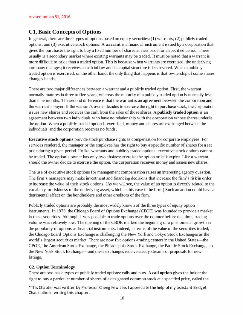
C1. Basic Concepts of Options In general, there are three types of options based on equity securities: (1) warrants, (2) publicly traded
options, and (3) executive stock options. A warrant is a financial instrument issued by a corporation that
gives the purchaser the right to buy a fixed number of shares at a set price for a specified period. There
usually is a secondary market where existing warrants may be traded. It must be noted that a warrant is
more difficult to price than a traded option. This is because when warrants are exercised, the underlying
company changes; it receives a cash inflow and its capital structure is less levered. When a publicly
traded option is exercised, on the other hand, the only thing that happens is that ownership of some shares
changes hands.
There are two major differences between a warrant and a publicly traded option. First, the warrant
normally matures in three to five years, whereas the maturity of a publicly traded option is normally less
than nine months. The second difference is that the warrant is an agreement between the corporation and
the warrant’s buyer. If the warrant’s owner decides to exercise the right to purchase stock, the corporation
issues new shares and receives the cash from the sales of those shares. A publicly traded option is an
agreement between two individuals who have no relationship with the corporation whose shares underlie
the option. When a publicly traded option is exercised, money and shares are exchanged between the
individuals and the corporation receives no funds.
Executive stock options provide stock purchase rights as compensation for corporate employees. For
services rendered, the manager or the employee has the right to buy a specific number of shares for a set
price during a given period. Unlike warrants and publicly traded options, executive stock options cannot
be traded. The option’s owner has only two choices: exercise the option or let it expire. Like a warrant,
should the owner decide to exercise the option, the corporation receives money and issues new shares.
The use of executive stock options for management compensation raises an interesting agency question.
The firm’s managers may make investment and financing decisions that increase the firm’s risk in order
to increase the value of their stock options. (As we will see, the value of an option is directly related to the
variability or riskiness of the underlying asset, which in this case is the firm.) Such an action could have a
detrimental effect on the bondholders and other creditors of the firm.
Publicly traded options are probably the most widely known of the three types of equity option
instruments. In 1973, the Chicago Board of Options Exchange (CBOE) was founded to provide a market
in these securities. Although it was possible to trade options over the counter before that time, trading
volume was relatively low. The opening of the CBOE marked the beginning of a phenomenal growth in
the popularity of options as financial instruments. Indeed, in terms of the value of the securities traded,
the Chicago Board Options Exchange is challenging the New York and Tokyo Stock Exchanges as the
world’s largest securities market. There are now five options-trading centers in the United States—the
CBOE, the American Stock Exchange, the Philadelphia Stock Exchange, the Pacific Stock Exchange, and
the New York Stock Exchange—and these exchanges receive steady streams of proposals for new
listings.
C2. Option Terminology
There are two basic types of publicly traded options: calls and puts. A call option gives the holder the
right to buy a particular number of shares of a designated common stock at a specified price, called the

revised on Jan 31, 2016
*This Chapter was written by Professor Cheng Few Lee. I appreciate the help of my assistant Bridget Chadziutko in writing this chapter. 11
exercise price (or striking price), on or before a given date, known as the expiration date. On the
Chicago Board Options Exchange, options typically are created for three-, six-, or nine-month periods.
All have the same expiration date: the Saturday following the third Friday of the month of expiration. The
owner of the shares of common stock can write, or create an option and sell it in the options market, in an
attempt to increase the return or income on a stock investment. A more venturesome investor may create
an option in this fashion without owing any of the underlying stock. This naked option writing exposes
the speculator to unlimited risk because he or she may have to buy shares at some point to satisfy the
contract at whatever price is reached. This is a serious if the value of the underlying asset has a high
degree of variability.
A put option gives the holder the right to sell a certain number of shares of common stock at a set price
on or before the expiration date of the option. In purchasing a put, the owner of the shares has bought the
right to sell those shares by the expiration date at the exercise price. As with calls, one can create, or
write, a put, accepting the obligation to buy shares.
The owner of a put or call is not obligated to carry out the specified transaction, but has the option of
doing so. If the transaction is carried out, it is said to have been exercised. For example, if you hold a call
option on a stock that is currently trading at a price higher than the exercise price, you may want to
exercise the option to purchase stock at the exercise price and then immediately resell the stock at a profit.
This call option is said to be in the money. On the other hand, if the call option is out of the money—that
is, the stock is trading at a price below the exercise price—you certainly would not want to exercise the
option, as it would be cheaper to purchase stock directly. At the money means that the stock price is
trading at the exercise price of the option.
An American option can be exercised at any time up to the expiration date. A European option can be
exercised only on the expiration date; this makes it simpler to analyze because its term to maturity is
known. Because of this simplifying factor, we will concentrate on the valuation of European options. The
factors that determine the values of American and European options are the same; all other things being
equal, however, an American option is worth more than a European option because of the extra flexibility
it grants the option holder.
Although our discussion in this section is limited to options on equities, many other kinds of securities
underlie publicly traded options. For example, people also trade options to buy or sell stock indexes,
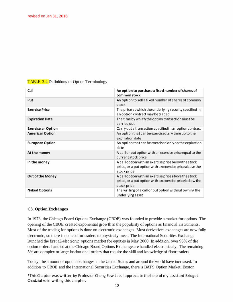
Treasury bonds, futures contracts, foreign currencies, and agricultural commodities. Table 3.4
summarizes the terms introduced in this section.
revised on Jan 31, 2016
*This Chapter was written by Professor Cheng Few Lee. I appreciate the help of my assistant Bridget Chadziutko in writing this chapter. 12
TABLE 3.4 Definitions of Option Terminology
Call An option to purchase a fixed number of shares of common stock
Put An option to sell a fixed number of shares of common stock
Exercise Price The price at which the underlying security specified in an option contract may be traded
Expiration Date The time by which the option transaction must be carried out
Exercise an Option Carry out a transaction specified in an option contract American Option An option that can be exercised any time up to the
expiration date European Option An option that can be exercised only on the expiration
date At the money A call or put option with an exercise price equal to the
current stock price In the money A call option with an exercise price below the stock
price, or a put option with an exercise price above the stock price
Out of the Money A call option with an exercise price above the stock price, or a put option with an exercise price below the stock price
Naked Options The writing of a call or put option without owning the underlying asset
C3. Option Exchanges
In 1973, the Chicago Board Options Exchange (CBOE) was founded to provide a market for options. The
opening of the CBOE created exponential growth in the popularity of options as financial instruments.
Most of the trading for options is done on electronic exchanges. Most derivatives exchanges are now fully
electronic, so there is no need for traders to physically meet. The International Securities Exchange
launched the first all-electronic options market for equities in May 2000. In addition, over 95% of the
option orders handled at the Chicago Board Options Exchange are handled electronically. The remaining
5% are complex or large institutional orders that require the skill and knowledge of floor traders.
Today, the amount of option exchanges in the United States and around the world have increased. In
addition to CBOE and the International Securities Exchange, there is BATS Option Market, Boston

revised on Jan 31, 2016
*This Chapter was written by Professor Cheng Few Lee. I appreciate the help of my assistant Bridget Chadziutko in writing this chapter. 13
(BOX) Options Exchange, C2 Options Exchange, ISE Gemini, MIAC Options Exchange, NASDAQ
OMX BX, NASDAQ OMX PHLX, Philadelphia Stock Exchange, NASDAQ Options Market, NYSE,
AMEX Options (American Stock Exchange), and NYSE Arca Options.
C4. Option Price Information
FIGURE 3.5Option Quotes for Johnson & Johnson, December 17, 2012
December 17, 2012
Johnson & Johnson (JNJ) Underlying stock price: 70.96
Expiration Call Strike Put
Last Chg Bid Ask Volume O pen
Int.
Last Chg Bid Ask Volume O pen
Int.
Dec 2012 3.50 +0.35 3.45 3.55 3 626 67.50 0.03 0.00 0.02 0.04 1 9402
Dec 2012 1.03 +0.28 1.04 1.10 10293 15316 70.00 0.09 -0.08 0.09 0.10 735 7237
Dec 2012 0.03 -0.03 0.03 0.01 99 10240 72.50 1.57 -0.39 1.53 1.59 113 1399
Jan 2013 3.57 +0.37 3.55 3.65 287 23980 67.50 0.11 -0.02 0.10 0.12 240 72991
Jan 2013 1.42 +0.21 1.41 1.43 313 70004 70.00 0.46 -0.15 0.46 0.47 444 10940
Jan 2013 0.27 +0.03 0.25 0.27 1188 33215 72.50 1.82 -0.32 1.78 1.83 308 7645
Mar 2013 6.20 +0.65 6.05 6.15 3 2418 65.00 0.26 -0.07 0.25 0.26 235 25415
Mar 2013 3.85 +0.30 3.80 3.85 53 47303 67.50 0.57 -0.14 0.56 0.58 179 12726
Mar 2013 1.92 +0.20 1.89 1.92 416 13686 70.00 1.34 -0.18 1.31 1.33 120 5866
Figure 3.5 presents options quotations for Johnson & Johnson. The price of Johnson & Johnson shares on
this date was $70.96. The first column gives the expiration month for each option. We have included
listings for call and put options with exercise prices ranging from $67.50 to $72.50 per share, and with
expiration dates in December 2012, and January and March 2013.
The next columns provide the closing prices, its change from the previous trading day, bid price, asked
price, trading volume, and open interest (outstanding contracts) of each option. Column 4 shows the Bid,
or the latest price offered by a market maker to buy a particular option. The Ask price in column 5 is the
latest price offered a market maker to sell a particular option. For example, the first contract traded on the
December 2012 expiration call with exercise price of $67.50. The last trade was at $3.50, meaning that an
option to purchase one share of Johnson & Johnson at an exercise price of $67.50 sold for $3.50. Each
option contract (on 100 shares) therefore costs $350.
Notice that the prices of call options decrease as the exercise price increases. For example, the December
2012 expiration call with exercise price $70 costs only $1.03. This makes sense, because the right to
purchase a share at a higher exercise price is less valuable. Conversely, put prices increase with the
exercise price. The right to sell a share of Johnson & Johnson at a price of $67.50 in December 2012 costs
$.03 while the right to sell at $70 costs $.09.

revised on Jan 31, 2016
*This Chapter was written by Professor Cheng Few Lee. I appreciate the help of my assistant Bridget Chadziutko in writing this chapter. 14
Option prices also increase with time until expiration. Clearly, one would rather have the right to buy
Johnson & Johnson for $70 at any time until January 2013 rather than at any time until December 2012.
Not surprisingly, this shows up in a higher price for the January 2013 expiration options. For example, the
call with exercise price $70 expiring in January 2013 sells for $1.42, compared to only $1.03 for the
December 2012 call.
CONCEPT QUIZ
1. What are the three types of options based on equity securities?
2. What is the difference between an American and a European option?
3. What is the difference between a put and a call option?
C5. Option Valuation
Let’s begin with a simple question. How much is a call option worth on its expiration date? The question
is simple because the imminent expiration makes the uncertain future movements of the price of the stock
irrelevant. The call must be exercised immediately or not at all. If a call option is out of the money on its
expiration date, it will not be exercised; it will become a worthless piece of paper.
On the other hand, if the call option is in the money on its expiration date, it will be exercised. The owner
can purchase stock at the exercise price and immediately resell if at the market price, if desired. The
option value is the difference between these two prices. On the call option’s expiration date, its value is
either zero or some positive amount equal to the difference between the market price of the stock and the
exercise price of the option.
C5.1 Basic Model
Symbolically, let P equal the price of the stock and X equal the exercise price of the option. The value of
the call, Vc, equals the maximum of zero or P minus X. This relationship can be written as:
Vc = Max(0, P – X) (3.1)
where Max denotes the larger of the two bracketed terms. For a put option (Vp), Vp = X – P if X > P, and
Vp = 0 if X ≤ P. This can be written as:
Vp = Max(0, X – P) (3.2)

revised on Jan 31, 2016
*This Chapter was written by Professor Cheng Few Lee. I appreciate the help of my assistant Bridget Chadziutko in writing this chapter. 15
The call position is illustrated in Panel (a) of Figure 3.1, which considers a call option with an exercise
price of $50, the call option is worthless, Vc = 0. The option’s value increases as the stock price rises
above $50. If, on the expiration date, the stock is trading at $60, then the call option is worth $10.
Panel (b) of Figure 3.1 is the mirror image of Panel (a); it shows the position of the write of the call
option. If the stock is trading below the exercise price on the expiration date, the call option will not be
exercised and its seller will incur no loss. However, stock is trading at $60, the seller of the call option
will be required to sell this stock for $50, that is, $10 below the price that could be obtained on the
market.
We have seen that once a call option has been purchased the holder of the option may obtain gains but
cannot incur losses beyond the initial premium payment. Correspondingly, the writer of an option may

revised on Jan 31, 2016
*This Chapter was written by Professor Cheng Few Lee. I appreciate the help of my assistant Bridget Chadziutko in writing this chapter. 16
incur losses but cannot achieve any more gains after receiving the premium. In both cases, the premium
represents the current value of the option. Further, there is not net gain; the profit gained by one balances
the loss of the other. Thus, options are zero-sum securities; they transfer wealth, rather than create it. To
acquire this instrument, the buyer must pay the premium to the writer. This value is the price paid to
acquire the chance of future profit, and therefore, it will reflect uncertainty about future market prices of
the common stock. Several factors that influence call option values are discussed in the next section. The
real value or attractiveness of options has to do with how options can transform risks. So it is not wealth
creation that gives options value but rather the risk transformation factor.
C6. Variables That Influence Call Option Value
Five factors influence the value of a call option: the market price of the stock, the exercise price of the
option, the risk-free interest rate, the volatility of the stock price, and the time that remains before the
option’s expiration date. We’ll examine the impact of these factors on call value next.
Market Price of the Stock. AE in Figure 3.2 shows the curvilinear relationship between a call option’s
value and the market price of the underlying stock. As already noted, the slope of this relationship
increases as market price becomes higher; eventually, each dollar increase in the price of the stock
translates into an increase in the value of the call option. In Figure 3.2, AB and CD represent the
maximum and the minimum value for the call option, respectively.
Exercise Price of the Option. Offered two otherwise identical call options on the same stock, you would
prefer the one with the lower exercise price. It would generate larger gains from any favorable movement
in the price of the stock than the option with the higher exercise price. Therefore, a lower exercise price
implies a higher call-option value, all other things being equal. In Figure 3.2, C represents the exercise
price. In addition, the locations of at the money, in the money and out of the money prices are also
presented.
Risk-Free Interest Rate. If a call option is eventually exercised, the holder of the option will reap some
of the benefits of an increase in the market value of the stock. The option holder will enjoy this gain
without having to pay the exercise price immediately. This payment will be made only at some future
time, when the call option is actually exercised. In the meantime, this money can be invested in
government securities to earn a no-risk return.
This opportunity confers an increment of value on the call option. All else being equal, a higher risk-free
interest rate should cause a greater call option value. Moreover, postponing the exercise of the option for
a longer time should increase the risk-free interest earnings. Accordingly, the risk-free interest rate should
help to determine a call option’s value in conjunction with the time remaining before the expiration date.

revised on Jan 31, 2016
*This Chapter was written by Professor Cheng Few Lee. I appreciate the help of my assistant Bridget Chadziutko in writing this chapter. 17
TABLE 3.6 Probabilities for Future Prices of Two Stocks
Less Volatile for Stock A More Volatile for Stock B Future Price (P) Prob (PR) (P)(PR) Future Price(P) Prob(PR) (P)(PR)
42 0.10 4.2 32 0.10 3.2 47 0.20 9.4 42 0.20 8.4 52 0.40 20.8 52 0.40 20.8 57 0.20 11.4 62 0.20 12.4 62 0.10 6.2 72 0.10 7.2 1.00 52.0 1.00 52.0
Volatility of the Stock Price. Suppose that you can purchase call options on either Stock A or Stock B
each with an exercise price of $50. Table 3.6 lists probabilities (PRi) for different market prices (Pi) on

revised on Jan 31, 2016
*This Chapter was written by Professor Cheng Few Lee. I appreciate the help of my assistant Bridget Chadziutko in writing this chapter. 18
the expiration date for each stock. Both mean expected future prices are $52.1 However, the price of Stock
B is far more likely to differ substantially from the mean than the price of Stock A. The price of such a
stock is said to be more volatile.
Following Equation 3.1, the expected payoff (EP) on the expiration date for a call option can be defined
as:
EP = ∑ (𝑃𝑅𝑖 ) × Max(0,𝑃𝑖 − 𝑋)𝑛𝑖=1 (3.3)
where Pi is the stock price per share at the ith state of nature, X is the exercise price, and PRi is the
probability at the ith state of nature.
The expected payoff on the expiration date for a call option on the more volatile stock is higher than the
expected payoff for a call option on the less volatile stock. The option on the less volatile stock will not
be exercised at a price below $50; for the three prices above $50, it exercise will result in payoff of $2,
$7, and $12. Therefore, following Equation 3.3, the expected payoff for the call option on the less volatile
stock (EPA) is:
EPA = (0.10)(0) + (0.20)(0) + (0.40)(2) + (0.20)(7) + (0.10)(12) = $3.40
Similarly, for a call option on the more volatile stock, EPB:
EPB = (0.10)(0) + (0.20)(0) + (0.40)(2) + (0.20)(12) + (0.10)(22) = $5.40
where 𝐸𝑃𝐵 is the = $5.40 expected payoff from the call option on the more volatile stock.
Although the mean expected future price is the same for the two stocks, the expected payoff from a call
option on the more volatile stock is higher. This conclusion is quite general. For example, it does not
require that the exercise price must fall below the expected future stock price.
Time Remaining to Option’s expiration. The above discussions of the risk-free interest rate and stock-
price volatility both suggest that a longer time remaining before an option’s expiration date should
accompany a higher call option value, all else being equal. Extra time allows larger gains from postponing
payment of the exercise price, and it permits greater volatility in price movements of the stock. These two
considerations operate together to increase the value of a call option.
Following the five variables just mentioned, black and Scholes derived the well-known option pricing
model presented in Appendix 3B1. In the following section, we will use these option concepts to discuss
option-like securities in some detail.
Option Valuation and related topics will be discussed further in Chapters 16, 17, 18, 19, and 20. Chapter
16 discusses Options and Option Strategies. Chapter 17 describes the Option Pricing Theory and Firm
Valuation. Chapter 18 explains the Decision Tree and Microsoft Excel Approach for Option Pricing
Model. Chapter 19 discusses the Normal. Log-Normal Distribution, and Option Pricing Model. Chapter
20 provides a Comparative Static Analysis of the Option Pricing Model. Chapter 24 also discusses
portfolio insurance and synthetic options.
1 Mean expected future price (MEFP) is calculated by the following formula:
MEFP = ∑ (P𝑖)(PR𝑖 )𝑛𝑖 = 1

revised on Jan 31, 2016
*This Chapter was written by Professor Cheng Few Lee. I appreciate the help of my assistant Bridget Chadziutko in writing this chapter. 19
1See Black, F. and M.Scholes, “The Pricing of Options and Corporate Liabilities,” Journal of Political Economy, Vol. 31, <ay/June 1973, pp.637-659.
CONCEPT QUIZ
1. What five factors determine an option’s value?
2. Why is the volatility of a stock important in valuing options?
3. Why is time to expiration important in valuing options?
D. Option-Like Securities Some corporate bond and stock issues take on the characteristics of options. Bonds constitute a fixed
claim on the corporation, while common stock confers a residual claim and a share in corporate
ownership. However, corporations also raise capital by issuing securities that are neither straight debt nor
straight equity. In this section, we will discuss the following option-like securities: warrants, callable
bonds, convertible securities, and risky corporate debt.
D1. Warrants
As mentioned earlier, a warrant constitutes an option to purchase a specific number of shares of common
stock at a stipulated price for a set period of time directly from the issuing corporation. Typically, a
warrant accompanies a bond issue, but it is detachable; it can be traded separately from the bond. A
warrant is essentially a call option written by the company that issues the stock. Its value is influenced by
the same factors that influence the value of a call option.
In this context, the value of a warrant at expiration (Vw) is defined by the following equation:
Vw = Max[0, NP – NX] (3.4)
where P and X are as defined in Equation 3.1 and N is the number of shares obtainable with each warrant.
Example 3.2: The Value of a Warrant at Expiration
Q: A warrant for a firm gives the holder the right to buy three shares of stock for $30. On the expiration
date of the warrant, the common stock of the firm is selling at $12 per share. What is the value of the
warrant at expiration?
A: Substituting the above information into Equation 3.4, we obtain:
VW = Max[0, (3)($12) - $30] = $6
Therefore, the value of the warrant at expiration is $6.00.
Why would a corporation include a warrant with bond issue? To the extent that the market puts a positive
value on the warrant, a bond with a warrant will be valued more highly than an otherwise identical
straight bond. By attaching the warrant the corporation can sell debt at a lower interest rate.
A corporation does not know, however, how much capital it eventually will raise when owners exercise
their warrants. The amount raised will be related directly to the profits generated by the business activity
of the corporation over the exercise period. If the corporation is relatively unsuccessful, its stock price is
likely to stagnate and the warrants will not be exercised. On the other hand, if the corporation is

revised on Jan 31, 2016
*This Chapter was written by Professor Cheng Few Lee. I appreciate the help of my assistant Bridget Chadziutko in writing this chapter. 20
successful and its stock price rises, the warrants are more likely to be exercised, generating additional
capital, presumably at a time when it is most needed to fund further growth.
This discussion ignores changes in the market as a whole, though. Even if the firm does not prosper,
general market movements could carry the stock price upward or downward and thus affect the
profitability of the warrant’s exercise.
FROM THE BOARDROOM: Too Clever by Half
In the twilight zone of structured finance, the sun has set on what was once a favorite derivative. The
Nikkei-linked bond offered investors a high fixed coupon plus a variable value on redemption that rose or
fell with Japanese share prices. About ¥3 trillion ($23 billion) of the bonds were issued, estimates
Bankers Trust, which arranged many of the deals, before crashing shares and frowning regulators put an
end to them. Now many rue the day they ever heard of this particular bright idea.
The Nikkei-linked bond was designed in the late 1980s, mainly to help Japanese life insurance
companies pay policy-holders a guaranteed form of return. This rate was far higher than could be earned
on yen bonds or cash at the time. Life insurers found it hard to earn enough even in Japan’s booming
stock market, for they were (and are) required to pay policy-holders out of income and most companies
paid their shareholders stingy dividends. Enter Nikkei-linked bonds.
The bonds usually carried coupons three or four percentage points higher than those on other yen
bonds of similar quality. In return for that extra income, the investor bet that share prices would not fall.
In the most popular form of Nikkei-linked bond, investors sold the issuer the right to redeem the bond in
the future at a price that was pegged to the performance of the Nikkei average. Generally issued as one-
to-three-year Eurobonds, these hybrid securities often were placed with a single investor.
The deals typically were geared three times. This meant that, for every 1% the Nikkei fell, the
amount of principal to be repaid would fall by 3%. The investor stood to lose all his principal if the index
fell by one-third—and this is exactly what happened. Most Nikkei-linked bonds were issued in 1989 and
early 1990, when the Nikkei was between 30,000 and 39,000. Most investors had lost just about all their
principal when the Nikkei fell to around 21,000 toward the end of 1990.
Faced with this nasty predicament, some life insurers returned to the firms which has arranged the
deals, including Bankers Trust and Salomon Brothers. The investors wanted a way to postpone taking a
loss on the bonds. The investment banks responded with a flurry of “rescue bonds,” until the finance
ministry put a stop to all the Nikkei bonds.
The “rescues” allowed investors to double their bet, in the misguided belief that share prices could
not keep falling. An investor who faced losing, say, 80% of his principal would, in effect, sell the bond
back to the firm that had arranged it, at 100% of its face value. The arranger concocted a new bond,
typically worth twice the face value of the old one and with the same sort of fixed coupon. The cost to the
investor of delaying the pain was reflected in the redemption price, however. For the bond to be redeemed
at face value this time, share prices had to rise, in most cases, by some 40%.
It was only when this second batch of deals began to go wrong (a few bonds were even “rescued”

revised on Jan 31, 2016
*This Chapter was written by Professor Cheng Few Lee. I appreciate the help of my assistant Bridget Chadziutko in writing this chapter. 21
twice) with the continuing slide in share prices that the finance ministry called a halt. At the end of 1991,
the Nihon Keizai Shimbum, Japan’s leading financial daily, notified the financial firms arranging the deals
it would no longer permit its Nikkei average to be used in Eurobond issues.
By then, insurers had had enough of these weird hybrids and the Tokyo stock market. Accordingly,
they took advantage of a brief New Year rally to sell a chunk of their Nikkei-linked bonds while the
option still had some time to run. Bankers Trust estimates there are now only about ¥500 billion of
Nikkei-linked bonds outstanding, and most of the rest expire by next March. A once-flourishing market
will be confined to a footnote in financial history—where many other vogue derivatives will one day
surely follow.
Source: The Economist, May 23, 1992, p.82. Copyright 1992 The Economist Newspaper Group, Inc. Reprinted with permission.
Further reproduction prohibited.
Why would a corporation include a warrant with a bond issue? To the extent that the market puts a
positive value on the warrant, a bond with a warrant will be valued more highly than an otherwise
identical straight bond. By attaching the warrant the corporation can sell debt at a lower interest rate.
A corporation does not know, however, how much capital it eventually will raise when owners exercise
their warrants. The amount raised will be related directly to the profits generated by the business activity
of the corporation over the exercise period. If the corporation is relatively unsuccessful, its stock price is
likely to stagnate and the warrants will not be exercised. On the other hand, if the corporation is
successful and its stock price rises, the warrants are more likely to be exercised, generating additional
capital, presumably at a time when it is most needed to fund further growth.
This discussion ignores changes in the market as a whole, though. Even if the firm does not prosper,
general market movements could carry the stock price upward or downward and thus affect the
probability of the warrant’s exercise.
Section 5 of Chapter 17 will discuss the valuation model of warrants in further detail.
D2. Convertible Securities
A convertible security is a bond or preferred stock issue that typically gives its holder the right to
exchange it for a stipulated number of shares of common stock of the issuing corporation during a
specified period of time. Therefore, convertible bonds and convertible preferred stock represent options to
the security holder. If the price of common stock rises sufficiently, holders of these securities will find it
profitable to exercise their conversion rights. As for a warrant, such a right will have some positive value
in the market, so the market will accept a lower coupon rate on the corporation’s convertible bonds then it
would demand for a bond with no conversion privilege.
Convertible bonds are especially attractive when management prefers to raise capital by issuing equity
rather than debt, but believes that transient influences have led the market to temporarily undervalue its
common stock. If this perception is correct, the stock price will rise and, as a result, debt will be
converted to equity. A convertible bond issue may offer an advantage over a bond issue with warrants
since managers can predict how much capital the issue will raise.

revised on Jan 31, 2016
*This Chapter was written by Professor Cheng Few Lee. I appreciate the help of my assistant Bridget Chadziutko in writing this chapter. 22
The exercise of a warrant raises further capital for the firm; conversion simply substitutes equity for debt.
The conversion of a bond issue for shares of common stock does not raise new capital, but it does
implicitly increase cash flow if the conversion occurs prior to the bond’s maturity date, by reducing future
coupon payments.
A further distinction between warrants and convertible bonds is that warrants are not callable, while the
issuer generally can call a convertible bond. The bondholder can be offered the option of converting it
within a short time period or surrendering it at a specific cash price. As with all callable bonds, investors
demand higher returns for callable, convertible securities. Firms are willing to pay this higher price in
exchange for management flexibility.
We have seen why a corporation might want to issue a hybrid security rather than straight debt and/or
equity. What about the investor? These securities may be particularly attrac tive when investors have
trouble assessing the riskiness of a corporation’s future business activities. If the corporation embarks on
a high-risk enterprise, holders of straight bonds will be in the unappealing position of gaining nothing if
the enterprise succeeds and facing greatly increased default risk if it fails.
Warrants or conversion privileges can restore some balance. By exercising a warrant or converting a bond
to stock, the bondholder can share in any success resulting from a risky venture. This reduces the
importance of assessing the future business risk of a corporation’s activities. Now we will discuss how the
conversion privilege can be determined.
Consider an issue of 20-year bonds with face values of $1,000. Each bond is convertible to 50 shares of
common stock and the current market price of the stock is $15 per share. The coupon rate on these
convertible bonds is 9.5 percent, while straight debt of the issuing corporation with similar terms
currently carries a rate of 12 percent. This issue can be called by the corporation, at a price of $1,050, at
any time after five years. How much do investors pay for the conversion privilege?
The number of shares that can be received in exchange for each bond is set by the conversion ratio; the
conversion ratio of the issue described above is 50 shares to one bond. Immediate conversion would
exchange a bond valued at $1,000 for 50 shares of common stock, so that the effective price of the stock
would be $20 per share. This conversion price, in general, equals:
Conversion price = Par value of bond
Conversion ratio
Many convertible bond contracts specifically state conversion prices. The conversion price of the example
bond exceeds the current market price of the shares by one-third. Obviously, it makes no sense to exercise
this conversion privilege immediately. However, that privilege may have some value due to the profit that
holders of the convertible bond can expect to earn if the price of the stock increases sufficiently.
The value of the conversion privilege is determined by computing the present value of the bond’s debt
element. Holding the bond to maturity, the bondholder would receive a stream of 20 annual payments of
$95, plus $1,000 at the end of Year 20. Discounting these payments at a rate of 12 percent gives a present
value of debt, PVD, of:

revised on Jan 31, 2016
*This Chapter was written by Professor Cheng Few Lee. I appreciate the help of my assistant Bridget Chadziutko in writing this chapter. 23
𝑃𝑉𝐷 = ∑$95
(1.12)𝑡 +$1,000
(1.12)20
20
𝑡=1
= $95 × PVIFA(12%, 20 years) + $1,000PVIF(12%, 20 years)
=$709.60 + $103.67 = $813.27
This often is called the straight bond value of the convertible bond. The market value of a convertible
bond is somewhat above the higher of the conversion or straight bond value, as shown in Figure 3.3.
Remember, however that the instrument may be worth more if the conversion privilege is exercised.
Since, at issue, the bond can be exchanged for 50 shares of common stock valued by the market at $15 per
share; its conversion value is 50 times $15 or $750. The bond value exceeds the conversion value, but it is
lower than the price of the bond. If the bond is issued at par, then the difference between the market value
of $1,000 and the larger of the straight bond value (line A in Figure 3.3) or conversion value is $186.73.
This represents the conversion premium, or the price (line B in Figure 3.5) that investors pay for the
conversion privilege. Section 5 of Chapter 5 will discuss this instrument in more detail.
As mentioned earlier, the conversion privilege is essentially a call option on shares of common stock, so
its value is influenced by all those factors that determine the value of call options. However, one
additional factor also has an effect. If the conversion privilege is exercised, the bond must be surrendered
in exchange for stock. Therefore, the exercise price per share of the call option is the market price of the
convertible bond divided by the conversion ratio. Over time, market forces will cause the price of the
convertible bond to vary, so the exercise price of the implicit call option also will vary.

revised on Jan 31, 2016
*This Chapter was written by Professor Cheng Few Lee. I appreciate the help of my assistant Bridget Chadziutko in writing this chapter. 24
D3. Callable Bonds
Corporate bonds often are issued with call provisions that entitle the issuer to buy back the bond from
bondholders at some later date, at a specified price. These securities are called callable bonds. We can
view the call provision as a call option held by the issuer of the bond. In this case, the excise price is equal
to the price at which the bond can be repurchased. In order for bondholders to allow the firm to hold a call
option on the security they own, they must be compensated with a higher coupon rate. Section 1 of
Chapter 5 will discuss this issue in more detail.
D4. Risky Corporate Debt
Sometimes, options are used to value risky corporate debt. Because of the limited liability of
stockholders, money borrowed by the firm is back, at most, by the total value of the firm’s assets. One
way to view this agreement is to consider that stockholders have sold the entire firm to debt holders but
hold a call option with an exercise price equal to the face value of the debt. In this case, if the value of the
firm exceeds the value of the debt, stockholders exercise the call option by paying off the bondholders. If
the value of the firm is less than the value of the debt, shareholders do not exercise the call option, and all
assets are distributed to the bondholders.
Black and Scholes (1973) have used the option pricing model to discuss the relationship between stock,
bonds, and firm values. Chapter 17 will discuss this issue in further detail.
CONCEPT QUIZ
1. Why would a corporation include a warrant with a bond issue?
2. Why might an investor prefer a hybrid security over straight debt?
3. Why are hybrid securities viewed as option-like securities?
4. What is the conversion price of a convertible bond?
D5. Earnings Per Share with Warrants and Convertibles
Warrants and convertible securities can change a firm’s earnings per share (EPS) and number of shares
outstanding. Investors, managers, accountants, and federal and state government agencies all watch the
earnings per share of a corporation. Earnings per share generally means net income after taxes, less
preferred stock dividends, divided by the weighted average number of shares of common stock
outstanding. In 1969, the Accounting Principles Board, a forerunner of the FASB, issued APB Opinion
No. 15, “Earnings per Share.” This ruling laid down the rules for calculating the earnings per share for
financial reporting purposes. In 1982, the FASB issued Statement No. 55, “Determining Whether a
Convertible Security Is a Common Stock Equivalent.” The accounting requirements set out in these
rulings provide alternative ways of calculating earnings per share if a company has outstanding
convertible securities, warrants, stock options, or other contracts that permit it to increase the number of
shares of common stock.
The EPS for a firm with a simple capital structure is called basic EPS. A simple capital structure has only
one form of voting capital and includes no potential equity, such as warrants or convertibles. The
existence of nonconvertible preferred stock does not create a complex capital structure.
A corporation that has warrants, convertibles, or options outstanding is said to have a complex capital
structure. The complexity comes from the difficulty of measuring the number of shares outstanding. This
is a function of a known amount of common shares currently outstanding plus an estimate of the number

revised on Jan 31, 2016
*This Chapter was written by Professor Cheng Few Lee. I appreciate the help of my assistant Bridget Chadziutko in writing this chapter. 25
of shares that may be issued to satisfy the holders of warrants, convertibles, and options should they
decide to exercise their rights and receive new common shares.
Because of the possible dilution in EPS represented by securities that have the potential to become new
shares of common stock, the EPS calculation must account for common stock equivalents (CSEs). CSEs
are securities that are not common stock, but are equivalent to common stock because they are likely to be
converted into common stock in the future. Convertible debt, convertible preferred stock, stock rights,
stock options, and stock warrants all are securities that can create new common shares and thus dilute (or
reduce) the firm’s earnings per share. APB No. 15 mandates the calculation of two types of EPS for a
firm with a complex capital structure: primary EPS and fully diluted EPS. It is useful to review the basic
accounting concepts dealing with income recognition and ownership at this point.
1. Basic EPS. The earnings available to stockholders are divided by the average number of shares actually
outstanding during the period.
2. Primary EPS. The earnings available to stockholders are divided by average number of common shares
plus the common stock equivalents (CSEs).
3. Fully diluted EPS. Earnings are handled in a manner similar to primary EPS, but all warrants and
convertibles are assumed to be exercised or converted. In other words, EPS is assumed to be at maximum
dilution.
The relationship between these three types of EPS can be presented as follows:
Type equation here.
EPS = Basic EPS – (Impact of CSE) – (CSE impact of all other dilutive securities)
It is interesting to speculate on whether the market will use primary EPS or fully diluted EPS in valuing
shares of stock. If the market expects holders of common stock equivalents to convert them into new
equity, then fully diluted EPS is likely to be more meaningful. If the market does not expect conversion,
then it is likely to treat convertible bonds like straight debt and focus on primary EPS with no adjustment
for new shares. In other words, the market is likely to use basic EPS in such cases.
Convertible bonds that have no chance of being converted are called hung convertibles. The idea here is
that if investors don’t wish to convert their bonds into the firm’s equity, the conversion price is hung. The
bond is worth more as a bond than it is worth converted into equity. APB No. 15 and FASB No. 55
require a firm to provide EPS information under either circumstance and let the market participant choose
which measure is more meaningful.
The financial analyst needs to identify the difference between two firms with a similar primary EPS value
and markedly different fully diluted EPS values. In general, hybrid securities in the capital structure cause
the difference.
Fully Diluted EPS
Primary EPS

revised on Jan 31, 2016
*This Chapter was written by Professor Cheng Few Lee. I appreciate the help of my assistant Bridget Chadziutko in writing this chapter. 26
CONCEPT QUIZ
1. How does the issuance of warrants or convertibles affect EPS?
2. What is fully diluted EPS? What is primary EPS?
E. Swap Contracts and Hedging
In addition to using forward, futures, and option contracts to hedge transactions or transaction exposure,
many corporations are engaging in what are called swap transactions to accomplish this. A swap
contract is a private agreement between two companies to exchange a specific cash flow amount at a
specific date in the future. If the specific cash flow amount is interest payments, then the contract is an
interest rate swap; if the specific amount of cash flows is currency payments, then the contract is a
currency swap. The first swap contract was negotiated between IBM and the World Bank in the early
eighties. Since that time, the swap market has grown to over $10 trillion.
E1. Interest Rate Swaps
An interest rate swap is a financial transaction in which two borrowers exchange interest payments on a
particular amount of principal with a specified maturity. The swap enables each party to alter the
characteristics of the periodic interest payments that it makes or receives.
The exchange might involve swapping a fixed-rate payment for a variable rate payment or one type of
floating rate for another. All swaps trade only interest payments made on underlying note values; no
principal payments need to change hands with a simple interest rate swap.

revised on Jan 31, 2016
*This Chapter was written by Professor Cheng Few Lee. I appreciate the help of my assistant Bridget Chadziutko in writing this chapter. 27
Figure 3.4 shows the cash flows of a simple interest rate swap for each of the parties involved. The two
primary parties to the swap are called counterparties. Usually, although not always, a financial
institution serves as an intermediary between the counterparties.
In this example, Company A exchanges a variable-rate debt for a fixed-rate debt. Company B trades its
fixed-rate debt for a variable-rate debt. The intermediary has no exposure to interest rate movements and
earns a fee of 0.1 percent, which is spread between the payments and the receipts of A and B.
In the typical interest rate swap, the counterparty with the fixed-rate debt pays a premium over the rate the
other counterparty initially paid on its variable-rate debt. This premium is based upon factors such as
terms of the swap, the creditworthiness of the counterparties, and the conditions in the market for fixed-
rate and variable-rate debt.
It is unusual for two companies to arrange an interest rate swap themselves. In most cases, intermediaries
act as brokers, dealers, or principals to the transaction. As a broker or dealer, the intermediary serves to
bring A and B together and collects an arrangement fee. However, in most swaps the intermediary acts as
a principal to both counterparties, assuming the credit risk in the event that one counterparty defaults.
When the intermediary acts as the principal to a swap, its compensation is in the form of an arrangement
fee and/or the spread between the terms of these two counterparties.

revised on Jan 31, 2016
*This Chapter was written by Professor Cheng Few Lee. I appreciate the help of my assistant Bridget Chadziutko in writing this chapter. 28
Firm A has a variable –rate debt with an interest rate of LIBOR (London Interbank Offer Rate) + 1%,
which is borrowed from the money market; Firm B has a fixed-rate debt with a fixed rate of 9.3%, which
is borrowed from the capital market. Through the intermediary, Firm A swaps its variable-rate debt for
Firm B’s fixed-rate debt at interest payment dates. This interest rate swap flowchart is presented in Figure
3.5.
The analysis of this swap is now presented in more detail.
From the information given in Figure 3.5, the interest rate cost of Firm A and Firm B and the fee of the
intermediary can be calculated as follows:
Firm A Intermediary Firm B
Pays Fixed 9.5% Fixed 9.4% Fixed 9.3%
LIBOR + 1% LIBOR + 1.1% LIBOR + 1.1% Receives LIBOR + 1.1% Fixed 9.5% Fixed 9.4%
LIBOR + 1.1%
Net Payment (income) Fixed 9.4% (.1%) LIBOR + 1%
After the swap, Firm A owns a fixed-rate debt with an interest rate of 9.4% and Firm B owns a variable-
rate debt with an interest rate of LIBOR + 1%. The intermediary earns a fee of 0.1 percent. Due to this
swap, Firm A has eliminated its interest rate exposure risk.
Firm A has entered into the swap, it has three sets of cash flows:
1. It pays FIXED 9.5% to Intermediary
2. It pays LIBOR + 1% to Money Market
3. It receives LIBOR + 1.1% from Intermediary
For Firm B, the swap could have the effects of transforming a fixed-rate loan into a floating-rate loan.
After it has entered into the swap, it has three sets of cash flows:
1. It pays FIXED 9.3% to Capital Market
2. It pays LIBOR +1.1% to Intermediary
3. It receives FIXED 9.4% from Intermediary
For intermediary, there are four cash flows:
1. It pays LIBOR +1.1% to Firm A
2. It pays FIXED 9.4% to Firm B
3. It receives FIXED 9.5% from Firm A
4. It receives LIBOR +1.1% from Firm B
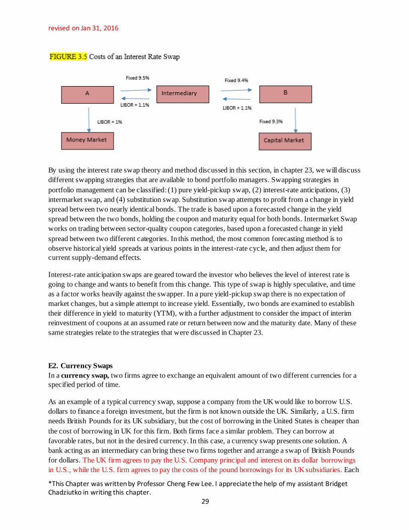
revised on Jan 31, 2016
*This Chapter was written by Professor Cheng Few Lee. I appreciate the help of my assistant Bridget Chadziutko in writing this chapter. 29
By using the interest rate swap theory and method discussed in this section, in chapter 23, we will discuss different swapping strategies that are available to bond portfolio managers. Swapping strategies in
portfolio management can be classified: (1) pure yield-pickup swap, (2) interest-rate anticipations, (3)
intermarket swap, and (4) substitution swap. Substitution swap attempts to profit from a change in yield
spread between two nearly identical bonds. The trade is based upon a forecasted change in the yield
spread between the two bonds, holding the coupon and maturity equal for both bonds. Intermarket Swap
works on trading between sector-quality coupon categories, based upon a forecasted change in yield
spread between two different categories. In this method, the most common forecasting method is to
observe historical yield spreads at various points in the interest-rate cycle, and then adjust them for
current supply-demand effects.
Interest-rate anticipation swaps are geared toward the investor who believes the level of interest rate is
going to change and wants to benefit from this change. This type of swap is highly speculative, and time
as a factor works heavily against the swapper. In a pure yield-pickup swap there is no expectation of
market changes, but a simple attempt to increase yield. Essentially, two bonds are examined to establish
their difference in yield to maturity (YTM), with a further adjustment to consider the impact of interim
reinvestment of coupons at an assumed rate or return between now and the maturity date. Many of these
same strategies relate to the strategies that were discussed in Chapter 23.
E2. Currency Swaps
In a currency swap, two firms agree to exchange an equivalent amount of two different currencies for a
specified period of time.
As an example of a typical currency swap, suppose a company from the UK would like to borrow U.S.
dollars to finance a foreign investment, but the firm is not known outside the UK. Similarly, a U.S. firm
needs British Pounds for its UK subsidiary, but the cost of borrowing in the United States is cheaper than
the cost of borrowing in UK for this firm. Both firms face a similar problem. They can borrow at
favorable rates, but not in the desired currency. In this case, a currency swap presents one solution. A
bank acting as an intermediary can bring these two firms together and arrange a swap of British Pounds
for dollars. The UK firm agrees to pay the U.S. Company principal and interest on its dollar borrowings
in U.S., while the U.S. firm agrees to pay the costs of the pound borrowings for its UK subsidiaries. Each

revised on Jan 31, 2016
*This Chapter was written by Professor Cheng Few Lee. I appreciate the help of my assistant Bridget Chadziutko in writing this chapter. 30
firm thus obtains the best possible rate and eliminates exposure to exchange rate changes by agreeing to
exchange currencies. Figure 3.6 illustrates the workings of a currency swap.
Figure 3.6 can be used to explain this action as: (a) principal exchange, (b) interest payment, and (c)
repayment. In this case, US firm and UK firm agree to exchange an amount of US dollars for an
equivalent amount of British Sterling. In a principal exchange, the UK firm pays the US firm an amount
of British Sterling and US firm equivalent amount of US dollars.
Consider a hypothetical five-year currency swap agreement between a US firm and a UK firm entered
into on March 1, 2014. We supposed the US firm pays a fixed rate of interest of 4% in sterling and
receives a fixed rate of interest of 5% in dollars from the UK. Interest rate payments are made once a year
and the principal amounts are $20 million and £15 million. This is termed a fixed-for-fixed currency swap
because the interest rate in each currency is at a fixed rate. The swap is shown in figure 3.6. Initially, the
principle amounts flow in the opposite direction to the arrows in Figure 3.6. At the outset of the swap, the
US firm pays $20 million and receives £15 million. Each year during the life of the swap contract, the US
firm receives $1 million (=5%*$20 million) and pays £.60 million (=4%*£15 million). At the end of the
life of the swap, its pays a principal of £15 million and receives principal of $20 million. We show these
cash flows in Table 3.7
Table 3.7 Cash flows to US firm in currency swap
Date Dollar Cash Flows Sterling Cash Flows
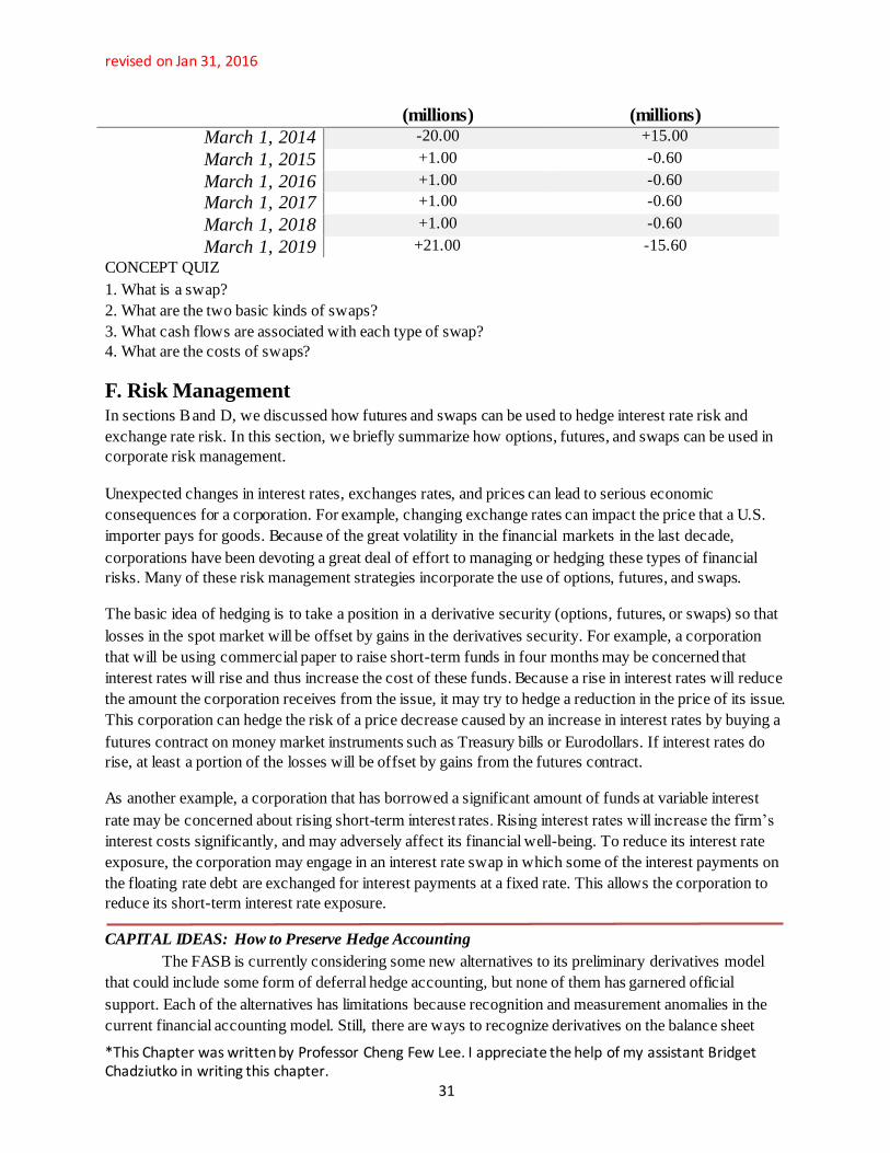
revised on Jan 31, 2016
*This Chapter was written by Professor Cheng Few Lee. I appreciate the help of my assistant Bridget Chadziutko in writing this chapter. 31
(millions) (millions)
March 1, 2014 -20.00 +15.00
March 1, 2015 +1.00 -0.60
March 1, 2016 +1.00 -0.60
March 1, 2017 +1.00 -0.60
March 1, 2018 +1.00 -0.60
March 1, 2019 +21.00 -15.60
CONCEPT QUIZ
1. What is a swap?
2. What are the two basic kinds of swaps?
3. What cash flows are associated with each type of swap?
4. What are the costs of swaps?
F. Risk Management In sections B and D, we discussed how futures and swaps can be used to hedge interest rate risk and
exchange rate risk. In this section, we briefly summarize how options, futures, and swaps can be used in
corporate risk management.
Unexpected changes in interest rates, exchanges rates, and prices can lead to serious economic
consequences for a corporation. For example, changing exchange rates can impact the price that a U.S.
importer pays for goods. Because of the great volatility in the financial markets in the last decade,
corporations have been devoting a great deal of effort to managing or hedging these types of financial
risks. Many of these risk management strategies incorporate the use of options, futures, and swaps.
The basic idea of hedging is to take a position in a derivative security (options, futures, or swaps) so that
losses in the spot market will be offset by gains in the derivatives security. For example, a corporation
that will be using commercial paper to raise short-term funds in four months may be concerned that
interest rates will rise and thus increase the cost of these funds. Because a rise in interest rates will reduce
the amount the corporation receives from the issue, it may try to hedge a reduction in the price of its issue.
This corporation can hedge the risk of a price decrease caused by an increase in interest rates by buying a
futures contract on money market instruments such as Treasury bills or Eurodollars. If interest rates do
rise, at least a portion of the losses will be offset by gains from the futures contract.
As another example, a corporation that has borrowed a significant amount of funds at variable interest
rate may be concerned about rising short-term interest rates. Rising interest rates will increase the firm’s
interest costs significantly, and may adversely affect its financial well-being. To reduce its interest rate
exposure, the corporation may engage in an interest rate swap in which some of the interest payments on
the floating rate debt are exchanged for interest payments at a fixed rate. This allows the corporation to
reduce its short-term interest rate exposure.
CAPITAL IDEAS: How to Preserve Hedge Accounting
The FASB is currently considering some new alternatives to its preliminary derivatives model
that could include some form of deferral hedge accounting, but none of them has garnered official
support. Each of the alternatives has limitations because recognition and measurement anomalies in the
current financial accounting model. Still, there are ways to recognize derivatives on the balance sheet

revised on Jan 31, 2016
*This Chapter was written by Professor Cheng Few Lee. I appreciate the help of my assistant Bridget Chadziutko in writing this chapter. 32
without eliminating traditional hedge accounting.
Why preserve hedge accounting? Hedging activities usually aren’t part of an enterprise’s central
operations, but neither are they merely peripheral transactions. The hedge accounting model for
traditional hedging activities has generally worked well for decades, producing financial statements that
reflect the economic substance of hedging transactions and management’s reasons for using derivatives.
The FASB’s approach prohibits deferring realized gains and losses, even to hedge the cost of a
long-term asset to be acquired in a future transaction. It effectively excludes firm commitments and
forecasted transactions from hedge accounting for many transactions because of the requirement to
recognize realized gains and losses immediately.
The FASB’s model includes derivative financial instruments that traditionally have been off the
balance sheet, such as futures, options, forwards and swaps. In addition, other instruments, whose
principal characteristics resemble those of off-balance-sheet derivatives, are included, even if they’re
recognized on the balance sheet. The board plans to expand the definition of a financial instrument to
include commodity-based contracts that entitle the holder to receive either a financial instrument or a
nonfinancial contract. And because the FASB’s model classifies all free-standing derivatives as trading
other than trading, it prescribes different accounting based on the instrument’s purpose, rather than the
type of instrument. It classifies trading derivatives as assets or liabilities and measures them at fair value,
and it recognizes changes in value in earnings as the changes occur. The model recognizes other-than-
trading derivatives as assets or liabilities and measures them at fair value. But it excludes from earnings
these derivatives’ changes in value and reports them in a separate component of equity until gains or
losses are realized.
Source: M.S. Joseph and S.A. Woltemath, “ How to Preserve Hedge Accounting,” Excerpted with permission from Financial Executive,
May/June 1995, pp. 32-35. Copy right 1995 by Financial Executives Institute, 10 Madison Avenue, P.O. Box 1938, Morristown, NJ 07962- 1938
(201)898-4600.
G. Summary
In this chapter, we discussed the basic concepts of futures, options, and swaps and how these instruments
can be used to hedge risk. In addition, the concept of options was used to illustrate the mechanics of a
number of securities that have option-like properties. Corporate securities, such as warrants, convertible
bonds, convertible preferred stock, callable bonds, and risky corporate debt all can be analyzed using the
basic principles of options. We also discussed the calculation of earnings per share for a company issuing
warrants and convertibles. We also discussed gold futures and another important hedging instrument, the
swap, including both interest rate swaps and currency swaps.
The main ideas discussed in this chapter are summarized as follows:
1. Futures contracts such as currency futures have similar characteristics as forward contracts. Both
forward and futures contracts can be used to hedge risk.
2. Two basic types of options are call option and put option. The value of call option depends on the
following five factors:
a. current stock price per share
b. exercise price of the option
c. risk-free interest rate
d. volatility of the stock price
e. time remaining to option’s expiration date

revised on Jan 31, 2016
*This Chapter was written by Professor Cheng Few Lee. I appreciate the help of my assistant Bridget Chadziutko in writing this chapter. 33
3. Firms frequently issue option-like securities. For example, warrants are long-term call options issued
by the firm; convertible bonds give the investor the right to buy the firm’s stocks in exchange for the
value of the underlying bonds. Callable bonds give the option right to the issuing firms instead of
investors.
4. Risky corporate debt issued by a firm can be regarded as an option contract. We can consider that
stockholders have sold the entire firm to debt holders but hold a call option with an exercise price equal to
the face value of the debt.
5. Swap contracts allow firms to exchange one series of future payments for another. Both interest rate
and currency swaps can be used to do risk management for a firm.
Key TermsAmerican option
Call option Callable bond Common stock equivalent (CSE) Complex capital structure
Conversion premium Conversion price Conversion ratio Convertible security
Counterparty Currency swap European option Executive stock options
Exercise price Expiration date
Forward contract
Futures contract Hung convertible Interest rate swap Maintenance margin
Margin requirement Marking to market Naked option writing Premium
Publicly traded option Put option Straight bond value Swap contract
Warrant
Self-Test Problems
1. Analyzing the Value of Convertible Bond
JoLee Corp. has a $1million, $1,000 par value, 9% semiannual convertible bond that is maturing in 5
years. The conversion price for the equity is $20 per share. Today, the common stock is selling for $18
per share. Similar convertibles have a stated nominal rate (APR) of 10%.
Calculate the conversion ratio, the conversion value, and the minimum price of the bond. As an
investor, what would you do with this bond? What is the value of the conversion privilege if the bond is
selling at $1,000?
A: Conversion ratio = Conversion ratio = Par value
Conversion price
= $1,000
$20/share
= 50 shares
Conversion value = Conversion ratio × Price per share
= 50 shares X $18/share
= $900

revised on Jan 31, 2016
*This Chapter was written by Professor Cheng Few Lee. I appreciate the help of my assistant Bridget Chadziutko in writing this chapter. 34
APR of 10% corresponds to a semiannual periodic rate of 5%
Bond value = ∑Interest
(1+𝑟)𝑡+
Par
(1+𝑟)𝑛𝑛𝑡=1
= $45 × PVIFA (5%, 10 periods) + $1,000 × PVIF (5%, 10 periods)
= $347.48 + $613.91
= $961.39
If the market price is below $900 per bond, you would buy the bond and convert it into common shares.
The value of the conversion privilege is the difference between $1,000 and the larger of bond value or
conversion value: $1,000 - $961.39 = $38.61.
2. Calculating the Value of a Warrant
On the expiration date of a warrant, the common stock of a firm is selling at $10 per share. The warrant
gives the holder the right to buy two shares of stock for $18. What is the value of the warrant at
expiration?
A: Using Equation 3.4, we obtain:
Vw = Max(0, NP – NX)
= Max (0, 2($10) - $18)
= $2.00/warrant
The stock is valued at $10 per share, or $20 for two shares. The exercise of the warrant to get two shares
costs $18; therefore, the warrant is worth $2.
Discussion Questions
1. Define the following terms:
a. executive stock option
b. call option
c. put option
d. exercise price
e. option premium
f. expiration date
g. naked option writing
h. in the money
i. out of the money
j. at the money
2. Distinguish between an American option and a European option.
3. What happens to the number of shares of stock outstanding when a call option is exercised?
4. What is the major difference between an option and a futures contract?
5. What is a convertible bond? Why would a corporation issue a convertible bond?
6. What is an interest rate swap?
7. Briefly explain how options are valued.
8. What is the relationship between the conversion ratio and the conversion price for a convertible bond?
9. Why will a convertible bond usually sell at a price above its value as equity or debt?
10. What is the difference between a warrant and a convertible bond?
11. What factors determine the value of a warrant?
12. Describe a situation in which a firm should consider issuing a convertible bond.
13. Describe a situation in which a firm should consider issuing warrants.

revised on Jan 31, 2016
*This Chapter was written by Professor Cheng Few Lee. I appreciate the help of my assistant Bridget Chadziutko in writing this chapter. 35
14. What is the conflict of interest when a manager with executive stock options is making capital
budgeting decisions concerning risky projects?
15. What is the problem with a corporate treasurer speculating with options and/or futures in order to
increase shareholder wealth?
16. Bankers do not need to explain the risks of using derivative instruments to sophisticated corporate
treasurers. Comment on the arguments for and against this statement.
Problems 1. Calculating Expected Value of Call Options
Find the expected value of a call option with an exercise price of $100 at the end of the period, given the
following information (current stock price is $100):
Probability Stock Price
0.4 $150
0.6 80
2. Calculating Value of Call Options
If a call option has an exercise price of $50, how much will it be worth on its exercise date (assuming no
transaction costs) if the price of the underlying stock is:
a. $30?
b. $50?
c. $80?
3. Call Option Value for Buyer and Seller
If a call option has an exercise price of $60 and the price of the stock is $40, what is the value of the call:
a. to the holder of the option?
b. to the seller of the option?
4. Expected Value of Call Options
Allison Merrick is considering two call options, each with an exercise price of $20 and identical in all
other respects except for the distribution of underlying stock values. The distribution of the values of the
underlying stocks of Companies J and K are given below:
Company J Company K
Future Stock Price Probability Future Stock Price Probability
$10 0.2 $5 0.1
18 0.3 17 0.3
22 0.3 25 0.4
25 0.2 35 0.2
Find the expected payoff for each call option and explain which one you would prefer.
5. Conversion Price of a Bond
LMW Company has issued convertible bonds that have a conversion ratio of 20 shares to one bond.
Compute the conversion price for a bond with a par value of $1,000. If the current market price for the
stick is $75 per share, does it make sense to convert? Why?
6. Price Conversion Privilege
Jones and Smith Company has just issued convertible bonds that have a coupon rate of 10 percent and a
conversion ratio of 25 shares to one bond. They mature in 20 years and pay semiannual coupons. If
similar straight debt has a nominal return of 14 percent, what price will investors pay for the conversion
privilege if the bonds currently are selling in par?

revised on Jan 31, 2016
*This Chapter was written by Professor Cheng Few Lee. I appreciate the help of my assistant Bridget Chadziutko in writing this chapter. 36
7. Price Conversion Privilege
The IKC Corporation has convertible bonds outstanding. The bonds have a coupon rate of 8 percent and a
conversion ratio of 50 shares to one bond. They mature in 10 years and pay semiannual coupons. If
similar straight debt has a nominal return of 10 percent, what price will investors pay for the conversion
privilege if the bonds currently are selling at par?
8. Calculating the Value of a Warrant
On the expiration date of a warrant, the common stock of a firm is selling at $25 per share. The warrant
gives the holder the right to buy five share of stock for $90. What is the value of the warrant at
expiration?
Appendix 3A: Single Stock Futures In this Appendix, we will learn about Single Stock Futures(SSF) and how these alternate securities can be
used by investors to increase their profitability while managing their exposure. Single Stock futures
possess many of the same qualities of traditional futures contracts, yet also have their differences. We will
look more into the nature of Single Stock Futures, as well as their advantages in this appendix.
Single stock futures are futures contracts on individual stocks. There are currently over 80 well-known
stock futures such as IBM, eBay, and Philip Morris. These futures products provide investors with a cost-
effective vehicle for participating in U.S. equities markets.
A stock futures contract is an agreement to deliver shares of a specific stock at a designated date in the
future, called the expiration date. Most stock futures contracts are not held until expiration because traders typically offset their position - selling if the trader is long or buying if the trader is short.
The price of an equity futures typically tracks the price of the underlying instrument nearly tick for tick,
so trading strategies followed in the stock market are generally transferable to the stock futures market.
Single stock futures may therefore be used with a broad range of trading strategies and for a variety of
portfolio management needs.
When a stock future is traded, both the buyer and seller put up a good faith deposit called margin. The
margin requirement for security futures is generally 20% of the underlying value of the securities,
although this requirement may be lower if the investor also holds certain offsetting positions in cash
equities, stock options, or other security futures in the same securities account.
3A.1 Nature of SSF Contracts
Each single stock futures contract represents 100 shares of underlying stock. That is the contract size used
at the London International Financial Futures Exchange (LIFFE) and by the Chicago Board Options
Exchange (CBOE) for equity options. There are no daily price limits for SSF contracts. Like other
securities that are exchange traded, physical delivery of underlying security takes place on the third
business day following the Expiration Day.

revised on Jan 31, 2016
*This Chapter was written by Professor Cheng Few Lee. I appreciate the help of my assistant Bridget Chadziutko in writing this chapter. 37
Figure 3A.1 SSF Quotes from OneChicago
Symbol Expiration
Month
Days to
Expiration
Future
BID
size
Future
BID
Future
ASK
Future
ASK
Size
Dividend Time
ONECHICAGO ETF Futures on 11-24-2014
XLF1D Dec 27 100 242.26000 24.3400 100 0.0000 11:23:59
XLE1D Dec 27 100 88.1500 88.2400 100 0.0000 11:24:00
SPY1D Dec 27 10 206.7000 207.3100 10 0.0000 11:23:31
QQQ1D Dec 27 50 104.3600 104.4400 50 0.0000 11:23:59
IWM1D Dec 27 10 117.2100 117.3600 10 0.0000 11:23:50
DIA1D Dec 27 100 117.6700 177.8000 100 0.0000 11:24:00 Top 10 Most Active Futures at ONECHICAGO on 11-24-2014
EA1D Mar 118 10 43.3300 44.2200 10 0.0000 10:06:33
AA1C Dec 27 0 0.0000 0.0000 0 0.0000 09:55:37
ALL1C Dec 27 0 0.0000 0.0000 0 02799 09:55:10
AUY1D Mar 118 500 4.0300 4.1000 500 0.0000 11:23:08
AXP1C Dec 27 0 0.0000 0.0000 0 0.0000 09:56:00
CCL1C Dec 27 0 0.0000 0.0000 0 0.0000 09:56:31
COH1D Dec 27 10 37.4100 37.4900 10 0.0000 11:24:00
COST1C Dec 27 0 0.0000 0.0000 0 0.0000 11:16:40
CS1D Dec 27 30 26.7600 26.8900 30 0.0000 11:23:38
CSCO1C Dec 27 0 0.0000 0.0000 0 0.0000 09:57:22
In Figure 3A.1, we see the market quotes for Single Stock Futures from OneChicago for November 24,
2014. Both tables show the trading of SSF on the OneChicago Exchange, the bottom table just
representing what stocks experience more frequent trading. The first column represents the symbol for
each of the SSF. In the bottom table, we see that there are quotes on Allstate (ALL1C), Cisco Systems
(CSCO1C), American Express (AXP), and many others. The second column, expiration month, states the month of expiration for each of the stock futures depicted, in this case either March or December. The
third column, days to expiration, expands on column 2 and provides a quantitative measure of the days
left in the futures contract. The fourth and seventh columns, Future Bid Size and Future Ask Size
describe the size of the futures contract in question. As we can see for the EA1D futures contract in the
second table, there is a bid/ask size of 10. The Future Bid illustrates the price that people are willing to buy the SSF contracts at, and the Future Ask is the price at which people are willing to sell. Looking at

revised on Jan 31, 2016
*This Chapter was written by Professor Cheng Few Lee. I appreciate the help of my assistant Bridget Chadziutko in writing this chapter. 38
the Dividend column, we see that most of the stocks do not offer a dividend, except for ALL1C. In the
following section we will see that when pricing single stock futures, we need to account for dividends by
subtracting them out of the equation due to the fact that SSF contract holders are not entitled to a dividend. The last column represents the time at which each trade occurred.
3A.2 Pricing Single Stock Futures Single stock futures values are priced by the market in accordance with a theoretical pricing model based
on a formula:
Futures Price = underlying stock price X (1+ annualized interest rate) - dividend)
For stocks that contain a dividend we get the following equation:
F = S ∙ (1 + r) – Div (3A.1)
Where F is the single-stock futures contract price, S is the underlying stock price, r is the annualized interest rate, and Div is the expected dividend.
Another valuation of single stock futures can be found through the following:
F = [S – PV (Div)] ∙ er∙(T-t) (3A.2)
Where F is single stock futures contract price, S is the underlying stock price, PV(Div) is the present
value of any dividends entitled to the holder of the underlying between T and t, r is the interest rate, and e
is the base of the natural log.
For stocks that do not contain a dividend we can price SSF using the following equation:
F = S ∙ (1 + r) (3A.3)
Where F is the single-stock futures contract price, S is the underlying stock price, r is the annualized
interest rate.
Another valuation of single stock futures can be found through the following:
F = S ∙ er∙(T-t) (3A.4)
Where F is single stock futures contract price, S is the price of the underlying (the stock price), T-t is the
days to expiration, r is the interest rate, and e is the base of the natural log.
Most of the time, single stock futures will trade at a premium to the stock price adjusted for the broker
loan rate. The premium reflects the interest earned on the capital saved by not posting the full value of
the underlying stock. Since futures holders are not entitled to collect dividends, the futures price must be
adjusted downward by the expected amount of dividend payments prior to expiration. In the case where a large dividend payment is expected, the futures contract may theoretically trade at a discount to the actual
cash price.
3A.3 Advantages of Single Stock Futures There are many advantages to an investor who chooses to use Single Stock Futures. Some of these
advantages are as follows:

revised on Jan 31, 2016
*This Chapter was written by Professor Cheng Few Lee. I appreciate the help of my assistant Bridget Chadziutko in writing this chapter. 39
Selling A Stock Short
One advantage to selling a stock short is the ease and diminished expense of taking a short position in a single stock. Selling a stock short in the stock market is relatively complicated and expensive. A short
sale in a stock necessitates locating the shares to borrow and paying the broker loan rate of interest. You
must then wait for an uptick to sell the stock short. Waiting for an uptick to sell a stock short in a
declining market can be frustrating and costly. By the time a particular stock upticks, it could be
substantially below the price at which you wanted it sold. However, in the futures market with the SSF contract, you can sell a stock short just as easily as you can buy one. When you sell a stock short using an
SSF contract, you don’t have to wait for an uptick. You can sell when you want, without going to the
trouble of finding the stock and without the expense of paying the broker loan rate of interest on the
shares borrowed.
Risk Management Selling SSF contracts can also greatly contribute to risk management in an investor’s portfolio with
possible tax benefits. Instead of selling specific stocks in one’s portfolio during market downturns, an
investor could sell an equal amount of shares in SSF as a hedge against his or her stock position. The
ability to hedge a particular stock facilitates holding onto the underlying position in the stock market for
longer periods of time, thereby potentially providing investors substantial tax savings in long-term versus short-term gains.
Speculation
An investor without owning any stock could use SSF to speculate outright on an anticipated increase or
decrease in the price of a stock.
Margins
One major difference between stocks and futures centers on the role of margins. For stocks, margins,
which are set by the Federal Reserve's Regulation T, have been at 50% for retail investors and 15% for
dealers since 1974. A stock investor buying on margin borrows the difference, and can either pay the loan
down, or offset it when the security is sold. Futures margins, which are set by the exchange, don't represent a down payment on an asset -- but are rather a performance bond from the investor to the
exchange clearinghouse. Margins vary quite widely as a percentage of the underlying asset, but generally
are quite low. For example, the underlying value of the S&P 500 future is hovering around $335,000, but
the initial margin for a speculator is only $23,438, or less than 7%. The futures investor doesn't have to
pay interest on the remaining 93%; indeed, futures investors can deposit T-bills and earn interest on 90% of the deposit with a 10% haircut in their margin accounts.
Cost Advantage
SSF are traded in 100-share blocks, virtually mirroring the price movement in the single stock on which
the futures contract is based. A $1 move in an individual stock equals $100 in an SSF contract. There is a big cost advantage here. In order to control shares in a stock, you need to post at least 50% margin and
pay interest on the balance. In SSF, all that is required is approximately 20%, or less than half the margin
required in the stock market. Additionally, there is no interest charge on buying or selling a stock on
margin in SSF. Essentially, you will earn or lose the same in an SSF contract as you would when buying
100 shares of stock.
Commission Savings
In all probability, the transaction costs in buying or selling a SSF contract amounts to less than buying or
selling the same 100 shares of stock in the stock market.

revised on Jan 31, 2016
*This Chapter was written by Professor Cheng Few Lee. I appreciate the help of my assistant Bridget Chadziutko in writing this chapter. 40
Spread Differentials
SSF offers investors additional investment strategies. For example, if an investor feels the price of one
stock will decline or rise in relation to another stock he or she can buy a SSF contract on one stock and sell a SSF contract on another, hoping to profit from the spread differential between the two stocks
anytime up to the contract’s expiration.
No Clearing Fees on Foreign Markets
Investor can also gain cross border exposure without the expense of going through foreign clearing systems. Will circumvent many of the difficulties faced by investors attempting to trade across
jurisdictional boundaries by providing access to UK, European and US shares on a single trading
platform.
Universal Stock futures transactions will be clear of costs of accessing settlement systems across
international borders
Greater Versatility
SSF allows a trader to potentially profit no matter what direction the market moves. If a trader is of the
opinion that the stock market is going to fall, a trader can sell a contract. A profit will be made if the
trader then buys that contract back later when the price decreases. This avoids the hassle of stock
borrowing.
Appendix 3B: The Black-Scholes Option Pricing Model Black and Scholes came up with a mathematical model to determine the value of an option. In this
appendix, we present an intuitive explanation of the model. The model can be understood in terms of the
following steps.
Step 1: The future stock price is constant over time.
Following Equation C4.1, if the stock price is constant over time, then the value of the call, Vc, is the
current price of the stock, P, less the present value of the exercise price, X. Mathematically, the value of
the call option is:
𝑉𝐶 = 𝑃 −𝑋
(1+𝑟)t (3B.1)
Equation 3B.1 assumes discrete compounding of interest. If continuous compounding (as discussed in
Appendix 6A of Chapter 6) is assumed, then Equation 3B.1 becomes:
Vc = P – Xe –rt (3B.2)
where e is a constant approximately equal to 2.71828.
Step 2: Assume the price of the stock fluctuates over time. In this case, we need to adjust Equation 3B.2
for the fluctuation associated with the uncertainty. IF we assume that the stock’s returns follow a normal
distribution, then both P and X in Equation 3B.2 can be adjusted for the uncertainty factor associated with
the fluctuation of the stock’s price over time. The call option pricing model thus becomes:
Vc = PN(d1) – Xe-rt N(d2) (3B.3)

revised on Jan 31, 2016
*This Chapter was written by Professor Cheng Few Lee. I appreciate the help of my assistant Bridget Chadziutko in writing this chapter. 41
where
𝑑1 =[ln (𝑃/𝑋)+(𝑟+.5𝜎2)𝑡]
𝜎√𝑡
𝑑2 = 𝑑1 − 𝜎√𝑡
r = risk-free interest rate
t = time until the option expires (in years)
Equation 3B.3 is the well-known Black-Scholes option pricing model. The adjustment factors N(d1) and
N(d2) represent the cumulative standard normal distribution function. N(d1) and N(d2) are probabilities
that a random variable with a standard normal distribution takes on a value less than d1 and d2
respectively. The values for N(d1) and N(d2) can be found by using a standard normal distribution table as
presented at the end of the book, in Table V on page 1122.
Equation 3B.3 can be used to find the theoretical value on January 12, 1995, of J&J’s call option expiring
in July 1995. In this case, we have X = $55, P = $54.875, σ = .1434, r = .0563, and t = .52 (years). Using
this information we can solve for d1 and d2.
𝑑1 =[ln(54.875 55⁄ ) + (. 0563 + .5(.1434)2)(.52)]
(. 1434)√.52
= .313
𝑑2 = .313 − (. 1434)√.52
= .21
To find the values for N(d1) and N(d2), we need to use the table in Table V. To find the cumulative normal
distribution function, we need to add the probability that Z is less than zero to the value given in the table
in Table AV. Because the standard normal distribution is symmetric around zero, we know that the
probability that Z is less than zero is .5, so N(d1) and N(d2) can be computed as:
N(d1) = P(Z < d1) = P(Z < 0) + P(0 < Z < d1)
= .5 + .1231
= .6231
N(d2) = P(Z < d2) = P(Z < 0) + P(0 < Z < d2)
= .5 + .0832
= .5832
Plugging this data into the Black-Scholes formula, we get:
Vc = 54.875(.6231) – (55)(.5832)e-(.0563)(.52)
= $3.04

revised on Jan 31, 2016
*This Chapter was written by Professor Cheng Few Lee. I appreciate the help of my assistant Bridget Chadziutko in writing this chapter. 42
The actual price of the option on January 12, 1995, was $2.75, as reported in The Wall Street Journal on
January 13, 1995.