Embed Size (px)
Citation preview

Support of Pavement Management Systems
At The Delaware Department of Transportation
Prepared for
Delaware Transportation Institute
And
Delaware Department of Transportation
By
Qingbo Zheng
And
David P. Racca
Center for Applied Demography and Survey Research
College of Human Resources, Education and Public Policy University of Delaware
Newark, DE 19716
December 1999

ii
The University of Delaware is committed to assuring equal opportunity to all persons and does not discriminate on the basis of race, color, sex, religion, ancestry, national origin, sexual preference, veteran status, age, or handicap in its educational programs, activities, admissions, or employment practices as required by Title IX of the Educational Amendments of 1972, Sections 503 and 504 of the Rehabilitation Act of 1973, Title VI and Title VII of the Civil Rights Act of 1964, the American Disabilities Act, Executive Orders 11246 and 11375 and other applicable statutes. Inquiries concerning Title IX, Section 503 and 504 compliance, Executive Order 11246 and information regarding campus accessibility and Title VI should be referred to the Affirmative Action Director, 305 Hullihen Hall, (302) 831-2835, (302) 831-4552(TDD).

iii
TABLE OF CONTENTS
LIST OF FIGURES ...................................................................................................................................................v LIST OF TABLES ....................................................................................................................................................vi
Introduction................................................................................................................................................................. 1
Part I Background of PMS ....................................................................................................................................... 3
Introduction of PMS.................................................................................................................................. 1
Why Is PMS Important ............................................................................................................................. 4
Experiences in Other States ..................................................................................................................... 5
FHWA Pavement Policy .......................................................................................................................... 6
AASHTO Guidelines ................................................................................................................................ 8
DelDOT PMS............................................................................................................................................. 8 Part II Foundations of PMS.................................................................................................................................... 11
A Fra mework of Pavement Management............................................................................................ 11
Data Collection......................................................................................................................................... 12
Pavement Condition Indicators ............................................................................................................. 14
Performance Modeling............................................................................................................................ 15
Pavement Performance Prediction Methodologies............................................................................ 17
Optimization ............................................................................................................................................. 19
Preventive Maintenance.......................................................................................................................... 20 Part III Support of DelDOT Pavement Management Systems Enhancements ............................................. 23
Introduction............................................................................................................................................... 23
Evaluation of OPC................................................................................................................................... 23
Determination of OPC ............................................................................................................... 24 Variability ..................................................................................................................................... 25 Errors and Outliers....................................................................................................................... 26 Yearly Difference ........................................................................................................................ 27 Comparison with Automated Measures of Districts .............................................................. 28
Pavement Performance Modeling......................................................................................................... 34
Factors Used to Predict Performance ....................................................................................... 34 Age ................................................................................................................................. 34 Pavement Types ........................................................................................................... 35 Structure Number......................................................................................................... 35 Model Procedure .......................................................................................................................... 36 Grouping of Highway Sections................................................................................. 36 Screening Procedure.................................................................................................... 37 Linear Regression Analysis ........................................................................................ 38 Non-linear Regression Analysis ................................................................................ 40

iv
Inclusion of Structure Number into Non-linear Analysis ..................................... 46 Improvement on Pavement Management Database............................................................... 51
Summary of Findings.............................................................................................................................. 52
A Review of Current Practices .................................................................................................. 52 A Review of Data Needed for PMS and Its Availability...................................................... 53 Evaluating the Current OPC and How It Relates to Age...................................................... 54 The Development of Pavement Performance Models ........................................................... 55
Reference................................................................................................................................................................... 57 Appendix A Correlation of OPC with Distress Types Appendix B OPC Rating Guide Appendix C Correlation of Pavement Family with Surface Type Appendix D Crosstabulation of Structure Number and Pavement Type

v
List of Figures
Figure 1 PMS Framework ........................................................................................................................ 11
Figure 2 Pavement Performance Curves ................................................................................................ 16
Figure 3 Maintenance Strategies ............................................................................................................. 20
Figure 4 Distribution of OPC................................................................................................................... 25
Figure 5 Scatterplot of OPC and Age..................................................................................................... 26
Figure 6 Percentage of Asphalt Transverse Cracking.......................................................................... 30
Figure 7 Percentage of Asphalt Fatigue Cracking................................................................................ 30
Figure 8 OPC and Roughness .................................................................................................................. 32
Figure 9 OPC and Ride Number.............................................................................................................. 32
Figure 10 Histogram of Residual............................................................................................................... 38
Figure 11 Linear Model for Rigid Family ................................................................................................ 39
Figure 12 Linear Model for Composite Family ...................................................................................... 39
Figure 13 Linear Model for Flexible Family ........................................................................................... 40
Figure 14 Pavement Conditions Forecasting Model.............................................................................. 41
Figure 15 Rigid Families in the North District........................................................................................ 43
Figure 16 Composite Families in the North District .............................................................................. 43
Figure 17 Flexible Families in the North District ................................................................................... 44
Figure 18 Composite Families in the South Disctrict ............................................................................ 44
Figure 19 Flexible Families in the South Disctrict ................................................................................. 44
Figure 20 Rigid Families in the Pooled Data........................................................................................... 45
Figure 21 Composite Families in the Pooled Data ................................................................................. 45
Figure 22 Flexible Families in the Pooled Data...................................................................................... 45

vi
LISTS OF TABLES Table 1 Pavement Performance Condition Indicators........................................................................ 15
Table 2 Example Comparison of the Effects of Alternative Maintenance Strategies................... 22
Table 3 OPC Scoring Based on Remaining Life ................................................................................. 24
Table 4 Distribution of Estimated Remaining Life ............................................................................. 27
Table 5 Statistical Summary of OPC Year Testing ............................................................................ 28
Table 6 Statistical Results from South District.................................................................................... 28
Table 7 ARAN Data Desciption............................................................................................................. 29
Table 8 Coefficients of Distress Types ................................................................................................. 31
Table 9 IRI and Roughness Categories................................................................................................. 31
Table 10 Family Distributions.................................................................................................................. 35
Table 11 Sample Outliers .......................................................................................................................... 38
Table 12 Statistical Parameters of First-order Linear Prediction Models ......................................... 41
Table 13 Statistical Parameters of Third-order Polynomial Prediction Models .............................. 42
Table 14 Dummy Variables for Family Classification......................................................................... 47
Table 15 Models Summary of Family Testing ...................................................................................... 48
Table 16 Coefficients of Family Testing ................................................................................................ 48
Table 17 Models Summary of Structure Number Testing................................................................... 49
Table 18 Analysis of Variance of Structure Number Testing............................................................. 49
Table 19 Coefficients of Structure Number Testing............................................................................. 50
Table 20 Coefficients Statistics of Flexible Family .............................................................................. 50

1
Introduction
This is the final report of the Delaware Transportation Institute Project "Support of the
Development of Pavement Management Systems, Part I" as prepared by the Center for Applied
Demography and Survey Research (CADSR) at the University of Delaware. It describes research
and analysis sponsored by the Delaware Department of Transportation (DELDOT) through the
DELDOT Pavement Management Team.
Over the last few years, DELDOT has initiated substantial efforts to improve decision
making in regards to the maintenance of the road network. These efforts include the
improvement of historic databases on pavement structure and conditions, analysis of pavement
condition rating schemes in use, and the development of multi-year prioritization tools for the
development of a multi-year prioritization capability to determine the timing and types of
pavement rehabilitation projects that would be most cost effective.
As part of these efforts DELDOT initiated contracts with Applied Pavement Technology,
Inc (APTech) and the Delaware Transportation Institute (DTI). The DTI portion of the work
conducted by CADSR supported the DELDOT Pavement Management Section and APTech in a
multi-phased project to provide enhancements to pavement management systems at DELDOT.
CADSR's work was focused in the following areas:
§ A review of current practices in pavement management systems.
§ A review of the data needed for PMS and its availability to support DELDOT initiatives.
§ An evaluation of the current Overall Pavement Condition (OPC) rating used by DELDOT
and its relationship to age, type, and other attributes of roads.
§ Development of performance models for Sussex and New Castle counties based on the data
provided by DELDOT.
§ Examination of Sussex County surface distress data provided by automated means.
§ Assistance with the development of pavement management databases and tracking systems.
This report describes CADSR's role and findings and is divided into three parts. Part I provides a
background of pavement management systems and includes highlights of the research and

2
literature review component of the project. Part II discusses the foundations of pavement
management systems in terms of the data collection, modeling, and optimization that are
involved. Part III discusses the specific work and analysis performed by CADSR in this project.
A summary of findings by CADSR is provided at the end Part III.

3
PART I - BACKGROUND OF PAVEMENT MANAGEMENT SYSTEMS
Introduction of PMS
The term “pavement management systems (PMS)” originally came into use in the late
1960s. In 1966, the American Association of State Highway Officials (AASHO), now referred to
as the American Association of State Highway and Transportation Officials (AASHTO), through
the National Cooperative Highway Research Program, initiated a study to make new
breakthroughs in the pavement management field. The intent was to provide a theoretical basis
for extending the results of the AASHO Road Test. As a result, researchers at the University of
Texas in 1968 began to look at pavement design anew, using a systems approach. Simultaneously,
independent efforts were being conducted in Canada to structure the overall pavement design and
management problem and several of its subsystems. A third concurrent keystone effort was that
of Scrivner and others at the Texas Transportation Institute of Texas A&M University in their
work for the Texas Highway Department. The work of these groups provides the overall historic
perspective for pavement management systems.
The term pavement management systems began to be used by these groups of researchers
to describe the entire range of activities involved in construction and maintenance of pavements.
The initial operational or “working” systems were developed. One of the largest efforts was
Project 123, conducted by the Texas Highway Department, Texas A&M University, and the
University of Texas. A series of reports and manuals have resulted from this research, beginning
with 123-1 in 1970. The project has produced many of the modern innovations in pavement
analysis.
At present there is no universally accepted definition of a pavement management system.
Haas and Hudson referred to it as the pavement functions “considered in an integrated,
coordinated manner”. PMS was defined by the Organization of Economic and Cooperative
Development (OECD) Expert Group as “the process of coordinating and controlling a
comprehensive set of activities in order to maintain pavements, so as to make the best possible
use of resources available, i.e. maximize the benefit for society”. (OECD report, 1987). In
AASHTO’s Guidelines for Pavement Management Systems , PMS is “a systematic approach that
provides the engineering and economic analysis tools required by decision makers in making
cost-effective selections of Maintenance, Rehabilitation, and Reconstruction (MR&R) strategies

4
on a network basis”. Corresponding with this definition, pavement management today has
become a concept that is mandated in federal legislation and implemented by state highway
agencies, cities, counties, and airports throughout the world. It has evolved from a concept with
little practical application into an established approach that can be used by engineers to make
more informed decisions, resulting in more optimal use of resources.
Pavement management activities and system components are generally focused at two
administrative levels termed the “network” and “project”(or individual) levels. Network level
analysis is of greater interest to the decision makers and budget directors and is doubtless the
most powerful of pavement management approaches, because it involves:
§ Identification and ranking of candidate pavements for improvements;
§ Network-level budgeting;
§ Long range budget forecasts;
§ Network-level pavement condition assessments;
§ Forecast of future conditions.
The project level, on the other hand, is concerned with more specific technical management
decisions for the individual projects. It involves:
§ Assessing the causes of deterioration;
§ Determining potential solutions;
§ Assessing benefits of the alternatives by life-cycle costing;
§ Ultimately selecting and designing the desired solutions.
Why is PMS important?
A systematic approach to pavement management is needed to provide factual information
on the present state and evolution of pavement conditions, and logical procedures for evaluating
repair options, taking into accounts as much as possible all of their economic advantages and
disadvantages (Hass and Hudson, 1987). In this way, PMS assists with the technical problems of
choosing optimal times, places, and techniques for repairing pavements and simultaneously,
providing those in charge of maintaining and improving roads with the data and other technical
justifications needed to secure political support for adequate road maintenance budgets and
programs. As described in the most recent FHWA “Pavement Policy for Highways”. “The
analysis and reporting capabilities of a PMS are directed towards identifying current and future
5
needs, developing rehabilitation programs, priority programming of projects and funds, and
providing feedback on the performance of pavement designs, materials, rehabilitation techniques,
and maintenance levels.”
This systematic approach has advantages over the common approach of using rules of
thumb and intuitive engineering judgment. In times of budget austerity, available resources must
be put to their best use, which means that all the practical options should be quantitatively and
economically evaluated to identify the best overall solution. A comprehensive pavement
management system supported by computerized tools to examine in detail the estimated costs and
benefits of various strategies can be very effective in making the best use of resources.
Experiences In Other States
While the initial introduction of PMS at the national level dates from the late 1970s and
early 1980s, most DOTs continue to rely on the experience of their maintenance, material, and
pavement engineers, rather than their PMS, to determine the performance of their maintenance
treatments and strategies. However, experience in the United States, where PMS took root during
the recent era of tight road budgets, shows that the benefits of systematic approaches to pavement
management have proven themselves in practice (Smith, 1992):
§ The Arizona Department of Transportation (ADOT) reports that PMS implementation
to optimize pavement rehabilitation expenditures enabled ADOT to save
approximately $300 million over a five-year period. These savings can be used to
expedite the construction of other badly needed capital improvements.
§ The California Department of Transportation (CALTRANS) reports that its priority
program of pavement rehabilitation projects based upon objective criteria established
by top management, has led to fewer instances where staff level (technical) decisions
are overridden by elected representatives. CALTRANS has been able to show, to the
satisfaction of its elected representatives, that the projects being funded are more
viable than those that are not, and its PMS has resulted in improved communication
between political and technical decision-makers.
§ Minnesota has a comprehensive, flexible and operational PMS in place, tailored to its
requirements. Among the key reasons for the successful development and

6
implementation were careful pre-implementation planning; strong support throughout
the department including senior management; a sound technical basis for the system
in terms of the data base, models, programs, and reporting functions; and a
commitment by those responsible for its systematic perspective.
§ A number of other state road administrations were able to argue successfully for
increases in their vehic le fuel tax rates, because they were able to show effectively
and objectively that previous program funding levels were insufficient to keep up
with deteriorating pavement.
These agencies employed different methods to improve the way they manage their
pavements but they all experienced a similar outcome. Because of the sound technical foundation
on which decisions were based, they were able to produce pavements with better performance
from available resources and ensure more effective technical input into the political decision-
making.
FHWA Pavement Policy for Highways
The Federal Highway Administration (FHWA) of the U.S. Department of Transportation
has focused attention on the use of pavement management concepts for cost-effective use of
highway funds. By co-sponsoring with the American Association of State Highway and
Transportation Officials (AASHTO) and the Transportation Research Board (TRB), numerous
conferences, workshops, and training activities have been conducted over the past 18 years.
The policy describes the scope and purpose of a PMS as providing the analysis and
reporting capabilities to highway administrators and engineers that include the ability to identify
current and future needs, develop rehabilitation programs, and prioritize programming of projects
and funds. Decisions are made in consideration of historic performance of pavement designs,
materials, rehabilitation techniques, and maintenance strategies. The policy advocates the
inclusion of full network level performance and trend information, covering all rural and urban
arterial routes under a transportation agency's jurisdiction. Certain data may be collected visually
for lower-order systems, but some degree of objective measurements should be made for high-
level systems. FHWA policy recommends that a state's PMS should address the following key
areas:

7
1. Inventory – An accounting of the physical features (number of lanes, widths, and
pavement type, shoulder information, functional classification, etc) of the roadway
network is essential.
2. Condition Survey – Measurement of the pavement condition (ride or roughness,
distress, structural adequacy, and surface friction) from which changes over time can
be determined.
3. Traffic Data – Traffic loading data are key elements that enter into analyses of
pavement performance and deterioration rates.
4. Database System – An effective, automated system for the storage and retrieval of
roadway inventory, condition, and traffic data is a critical feature of a PMS. A means
of linking data to physical locations is required to permit the incorporation of
maintenance management systems data and other data sources (bridges, accidents,
railroads crossing, etc.) into the PMS.
5. Highway Performance Monitoring System (HPMS) – Due to similar data needs,
coordination between the PMS and HPMS activities are encouraged.
6. Data Analysis Capabilities – The ability to effectively manipulate and use the
information in the database to produce useful reports for decision makers is probably
the most important capability of a PMS. Reports such as traffic analysis, network
trends, project programming, project ranking, and project selection strategy are
examples of the type of output needed by decision makers. An operational PMS will
enhance communication among planning, design, construction, maintenance,
materials, and research activities. As data is added over a longer time period, a PMS
can be used to develop evaluations of materials and designs in relation to traffic
loading and environmental conditions.
The policy required each state highway agency to have an operational PMS within a
reasonable time, not to exceed 4 years from the January 1989. The FHWA field offices
periodically monitor implementation progress and assess adequacy of each state’s PMS with
regard to quality of data collected, reports produced, and use in strengthening the pavement
program.

8
AASHTO Guidelines for Pavement Management Systems
AASHTO guidelines describe the various components of a PMS that are required for its
development and implementation, and how the PMS products and reports can be used as strategic
planning and programming tools. The guidelines suggest seven conditions necessary for the
development, implementation, and operation of a PMS.
§ Strong commitment from top management and coordination throughout the department.
§ A steering committee that exclusively deals with organizational and political problems.
§ PMS Staff including one person who will be the lead PMS engineer with full time
responsibility for managing, coordinating, and operating the PMS.
§ System selection or development including good data, good analysis, and effective
communications.
§ Demonstration of PMS on a limited scale.
§ Full-scale implementation – The pavement management team established earlier is very
important to successful implementation.
§ Periodical review and feedback.
DelDOT PMS
DelDOT Division of Highways is responsible for the maintenance of 4,765 miles of
public roads in Delaware. Of this mileage, 221 miles are multilane highways. Most of the
necessary funds for construction, reconstruction, rehabilitation, and maintenance of these roads
are allocated from the Delaware Transportation Trust Fund. This statewide roadway network
represents a tremendous investment. The preservation and management of these facilities is vital
to the economy of the state, and is a key responsibility of the Department. Increases in traffic,
both in numbers of vehicles and in wheel loads, along with rising costs and reduced resources,
results in significant challenges to administrative and engineering personnel.
A systematic approach to the management of the pavements is needed to provide
engineering and economic analysis tools required by decision makers in making cost-effective
selections of Maintenance, Rehabilitation, and Reconstruction (MR&R) strategies on a network
9
basis.
DelDOT has recognized this need since 1980s and has made significant progress toward
PMS development. In 1980, prior to the Federal guidelines, DelDOT management supported the
concept of PMS and appointed a PMS Steering Committee. Recommendations from this
committee led to improvements in data collection, the formation of a Pavement Management Unit
within the Office of Planning and Programming (now Division of Planning), and the designation
of a full-time Pavement Management Engineer. The Office of Planning and Programming, and
the Pavement Management Unit were instrumental in the development of a priority process for
selecting projects to be included in annual highway programs. However, the process did not
include some of the important features of a PMS such as forecasting, graphic reporting,
budgeting, and optimizing capabilities, and had some less desirable features:
§ There was an inability to forecast pavement conditions and needs.
§ The process was very labor intensive. Information for decision-making was located in
different data files and the analysis required both manual and computer efforts.
§ The process was based largely on more subjective evaluations of road condition, and
rules of thumb. Rating and prioritization of projects was still a "worst first" approach
with practically no consideration for preventive maintenance.
In 1991, in response to the requirements of Congress's Intermodal Surface Transportation
Act, DelDOT contracted with the consulting firm PCS/Law, to conduct state-of-the-art
engineering and economic analysis and to provide cost-effective management tools for the entire
network of paved roads and streets under DelDOT's jurisdiction. The initial project concentrated
on determining the specific DelDOT needs, desires, and objectives as they pertain to the PMS and
the preparation of a work plan responding to these objectives. As the work plan advanced,
DelDOT accepted PCS/Law's proposal to develop DelDOT PMS into multi-modal transportation
facilities. This project lasted several years but was discontinued in 1996. Several issues were
identified that needed to be addressed:
§ Limited availability of fiscal resources and technical know-how to support PMS once
implemented.
§ The absence of an agency-wide data base system and a complete historical pavement
database.

10
§ Inadequate identification of the needs and anticipated costs and benefits derived from
the project.
§ Political disruption of the PMS's consistency and uniformity
In order to consistently maintain and rehabilitate the pavement network, DelDOT
contracted with Applied Pavement Technology, Inc (APTech) and the Delaware Transportation
Institute (DTI) to evaluate the information available for the development of PMS components and
enhance the existing capabilities.
The first phase of the study conducted by APTech was completed in December 1997. The
study (APTech report) concentrated on the following areas of interest:
§ Data management – including the identification of the types of the data required to
support the pavement management efforts, procedures for obtaining the information, and
processes to ensure the consistency and quality of the data used.
§ Pavement performance models – including enhancements to the existing condition rating
methods, the development of agency-specific pavement performance prediction models,
and the establishment of preventive maintenance and rehabilitation treatments, triggers,
costs, and impacts.
§ Implementation/training – including the integration of the tools into the operational
processes that exist within DelDOT.
The findings from the first phase of the study will be further investigated in Phase II,
during which APTech will work with DelDOT Pavement Management to further develop
performance models and to implement pavement management computerized tools.

11
PART II - FOUNDATIONS OF PMS
A Framework of Pavement Management
Perhaps the most relevant research toward defining the components of a pavement
management system was conducted by OECD (Organization of Economic and Cooperative
Development) Expert Group’s study, which laid the foundation for cooperative research across
countries. The scope and objectives of PMS developed by OECD has been generally accepted by
a number of countries in North America and Europe. Students of PMS from different countries all
agree that the pavement maintenance procedure consists of four steps or processes as shown in
figure 1.
1. Data collection
2. Models/analysis
3. Criteria /optimization
4. Consequences/implementation
Figure 1 PMS Framework
Steps Elements - Structural conditions of pavements Data - Functional conditions of pavements Collection - Traffic condition (flow and axle load) - Costs and benefits (user, social)
Models - Performance predictions of pavements data Analysis - Distress predictions of pavements base - Costs and benefits of traffic operation - Costs and benefits of pavement operation
Criteria - Min. functional conditions of pavements Optimization - Min. structural conditions of pavements
- Min. overall costs or max. net benefits - Consequence - Necessary funding level Implementation - Schedule of maintenance works

12
Data Collection
The objective of data collection is to keep track of the actual condition of roadways and
record the condition in an objective and precise manner. Performance modeling depends on a
database reflecting structural and functional conditions. When conducting the data collection
procedure, the following elements are considered as important factors:
Variability
Variability of pavement surface distress measurements have always been an area of
significant concern. When conducting evaluations of distress data manually (with raters observing
the pavements in question, interpreting what they see and recording on paper) the data is subject
to all of the human errors associated with such a process. To minimize the impact of such human
errors on the important performance data, sophisticated equipment has been developed to
eliminate as much of the human interpretation as possible.
The variability associated with distress data is dependent on such issues as season of
collection, lighting, surface moisture, human experience and training as well as distress type,
severity, and amount. To adequately quantify the precision and bias, a detailed experiment to
evaluate the errors inherent in the different distress data collection methodologies is required.
Examples of such experiments can be found in SHRP’s Distress Identification Manual for the
Long-Term Pavement Performance Project and Guidelines for Pavement Management Systems
by AASHTO.
Measurement Errors
With any study, variables must be measured in order for analyse to be conducted and
conclusions drawn. Measurement is always accomplished with a specified device or procedure,
which will be referred to as an instrument (Carmines and Zeller, 1979). No matter what
instrument is used, there is always some degree of error associated with it. Error comes from
several sources including: the limits of precision of an instrument, idiosyncratic tendencies of the
person conducting the rating, bias in the design of an instrument, and simple errors in the way a
person uses the instrument. There are two types of errors, random error and bias. Random error
occurs when errors are nonsystematic and are as frequently in one direction as any other, and thus
values vary uniformly around the real or true score of the variable. Bias occurs when the errors
tend to be in one direction more than another.

13
Random error causes data collected in a study to be less than precise. However, if one
makes certain assumptions about the error component of measurement, one can use statistical
procedures to circumvent this problem. Bias is far more problematic than random error. Since
bias tends to be in one direction, there is no simple process to average out its effects. There may
be instances in which it is possible to estimate the magnitude and direction of bias and to adjust
for it.
Reliability
Reliability is a crucial characteristic of measurement and refers to the consistency of a
measuring device or rater. In other words, questions can be asked like: (1) does the instrument
always come up with the same score or number when the true value is the same? (2) Does the
rater always have the same degree of visual accuracy of rating the object?
Validity
Validity of an instrument or procedure means that it measures what it is designed to
measure. Validity is, in reality, complicated because raters are not always precise in their
meanings of concepts and rarely have standards for comparison. A valid measure of pavement
status would consist of a composite of structural and functional factors. But the question is how
should they be combined? The definition of a pavement condition index is usually elusive.
Generally an index is taken as part of a theoretical framework and establishes that certain
hypothesized relationships exist between the examined indicator and other variables. As one finds
that hypothesized relationships are supported, evidence for validity accumulates. Many agencies
use the International Rating Index (IRI) mainly because IRI has been tested by AASHTO and has
been accepted as a valid measurement. When none of the hypotheses are being upheld, either the
instrument is invalid or the theories are wrong. Through the collection of evidence over time, a
case is built for the validity of the measures, which are dependent upon theoretical models and
hypotheses.
Frequency
The frequency at which a highway agency collects pavement condition data, depends
primarily upon how often they need current data, budget restrictions, and the availability of

14
trained personnel (Wang, 1998). Some pavement management systems require annual evaluation
of pavement condition while others conduct pavement condition assessments once every two
years. Nationally, it is common practice to inspect the Interstate pavements at least annually and
other state maintained routes every other year.
However, the fact that the agency may collect pavement condition data every one, two, or
three years does not necessarily mean that it inspects all of their pavements or inspects the entire
length of a single pavement. Indeed, such a policy would often prove to be too time-consuming
and too costly. A practical approach is to sample intervals along a pavement based on a statistical
design aimed at achieving a prescribed level of confidence in the reported data as well as
specifying which pavements should be inspected. For example, the following criteria to select
pavements for inspection could be used:
1. Control sections which are tested every year to ensure consistency in the data;
2. Pavements with an index which exceeds a prescribed level on any of their failure
mode listings for the previous year;
3. Sections requested for testing by the district personnel, because of specific distress
conditions;
4. Pavements that have not been tested for a period of 3 years.
Pavement Condition Indicator
Whatever strategy is adopted for pavement management, it becomes important to assess
the pavement’s structural and functional qualities in a scientific, well-defined way. There are
generally two philosophies of achieving that goal. One way is to combine attributes in a specific
manner to determine a single pavement condition index universal to each section. By doing so, it
is important to note that the index be objective and reflective of the real-world pavement status
since the ultimate effectiveness of the decision is based upon the validity of this single index.
Equally important, data should be updated on a periodical basis in order to be reflected in the
index. The other philosophy is to use more than one condition indicator in decision trees, to
prioritize and coordinate between difference indices and condition states, or to tabulate a
pavement condition matrix. In this case there are usually several indices related to the extent of
various types of surface distress.

15
While some agencies use multiple indexes to establish priorities between several
pavements in need of repair, aggregation of pavement condition data into a single rating number
is widely used to support project and network level decisions in pavement management. To
characterize each pavement condition attribute and its time-decay relationship with traffic, age,
climate, and other variables, various models have been developed. Table 1 introduces a number
of condition indicators being adopted by several state agencies.
Table 1 Pavement Performance Condition Indicators
DOT Index Index Range Models
Alaska SCI N/A SCI=1.38(Rutting)2 + 0.01 (Alligator Craking +Full Width Patching)
Arizona “Rate” 0-5 Rate=Cracking+0.2(Roughness)+2(Rutting)+0.0015(Average Maintenance Cost for last 3 years)
Canadian DI 0-180
(1)DI=5(2(Severity of Raveling)+(Extent of Raveling)+Σ(2(Severity of Distress )+(Extent of Distress) (they are measured on a scale of 0 to 4) (2)DI=127+5.64Age-18.6(Percentage of Asphalt Cement Content in the Surface Course)-5.88log10
Average Annual Daily Traffic
(this is a prediction model)
Indiana PSI 0-5 PSI=4.7-0.065(Age)-0.000006(Average Annual Daily Traffic)-0.46(Pavement Types-1 for Concrete 0 for Bituminous)
Pennsylvania SDI 0-100 SDI=0.1(Excess Asphalt) +0.13(Raveling)+0.2 (Block Cracking)+0.25(Transverse/Longitudinal Cracking)+0.05 Edge Deterioration) +0.12 (Widening Dropoff)+0.15(Rutting)
Notes: DI --- Distress Index
PSI --- Present Serviceability Index SCI --- Surface Condition Index SDI --- Surface Distress Index
Performance Modeling
Performance modeling refers to the activity that patterns and predicts the deterioration of
pavement conditions with accumulating use, based on comprehensive evaluation of the structural
and functional characteristics of the pavement in service, deterministically and/or empirically. A

16
typical performance curve, relating the pavement condition rating to the age of the pavement, is
shown as an example in figure 2.
Figure 2 Performance Curve
Condition Indicator
Routine maintenance
Warning Level
Intervention Level
Maintenance period
Years
Being able to predict the condition of pavements is the most essential activity to the
management of pavements at the network and the project levels, both technically and
economically. In fact, the models play a crucial role in several aspects of the PMS, including
financial planning and budgeting as well as pavement design and life cycle economic analysis.
First, models are used to predict when maintenance should be required for individual road
sections and how to prioritize competing maintenance alternatives. Second, by virtue of its
prediction capability, the model enables the agency to estimate long-range funding requirements
for pavement preservation and to analyze the consequences of different budgets on the condition
of the pavement network. Third, because the models attempt to relate the influence of predicting
variables to pavement distresses or to a combined performance index, they can be used for design
as well as the life-cycle economic evaluation.
Pavements are complex physical structures responding in a complex way to the
influences of numerous environmental and load-related variables and their interactions. A
prediction model, therefore, should consider the evolution of various distresses and how they may
be affected by both routine and planned maintenance. Such an approach is so highly complex

17
that a compromise procedure combining a strong empirical base and a mechanistic approach is
adopted to achieve a reliable model. The empirical base includes time-series pavement condition
data compiled on pavements exposed to different environmental and loading conditions. With
regard to mechanistic principles, interactions between traffic loading and pavement strength
parameters, between loading and pavement deflections, and so on, are observed and included
when significant. These considerations dictate the model form and provide guidance in the
selection of the independent variables for inclusion in the predic tion model.
Pavement Performance Prediction Methodologies
Performance is the “ability of a pavement to fulfill its purpose over time”(AASHTO
Guidelines). A performance prediction method is “a mathematical description of the expected
values that a pavement attribute will take during a specified analysis period” (AASHTO
guidelines). Prediction models provide parameters to pavement management optimization so that
they can base the selection of future MR&R programs on the forecasted conditions.
Several methods of studying performance have been used by state agencies in the past
decade:
§ Performance curves: A performance curve defines variations of pavement attributes
over time. State agencies create performance curves for their particular conditions.
A bituminous pavement with high traffic and low subgrade strength may have a
different performance curve than a concrete pavement with low traffic and medium
subgrade strength. A performance curve normally relates expected relationships
between serviceability and age. These relationships are commonly estimated using
regression, include structural capacity versus age, skid resistance versus age, and a
measure of distress versus age.
§ Nondestructive testing (NDT): O’Brien, Kohn and Shahin studied Prediction of
pavement performance using NDT results. The NDT model was originally used by
several states. Several variables were included in this model: pavement type,
condition rating, NDT information, pavement construction, traffic information, and
pavement layer thickness. The independent variables were pavement construction
history, a weighted traffic variable, and NDT deflection parameters. The pavement
construction history was reflected in three pavement layer age variables: time since

18
last overlay, time from construction to first overlay, and total pavement age. The
NDT parameters were a normalized deflection factor given by the slope of the
deflection basin and a measure of the deflection basin area. The traffic variable
included in the prediction model is the natural logarithm of current traffic count
weighted by traffic type. The relevant significance of each variable group was 60
percent for the age variables, 30 percent for the NDT variables, and 10 percent for the
traffic variable.
§ Regression Analysis: Regression Analysis is the approach that is most commonly
used. A General Linear Model or polynomial model procedure is often used to
develop a linear regression equation. In most regression analyses, the fit of the
model is described by an R-square (R2) value. The R2 value is based on sample
correlation coefficients that indicate the strength of the developed relationship
between the dependent variable and independent variables when compared to the
observed data. R2 may then be interpreted as the proportion of total variability in the
dependent variable that can be explained by the independent variables. The R2 can
range from zero to one with the higher number indicating a better fit of the model to
the actual data.
§ Empirical-Mechanistic Model: This model is based on the assumption that a
prediction model should consider the evolution of various distresses and how they
may be affected by both routine and planned maintenance. However, this approach is
so complex that a compromise procedure combining a strong empirical base and a
mechanistic approach is adopted to achieve a reliable model. The empirical base
includes time-series pavement condition data compiled on pavements exposed to
different environmental and loading conditions. With regard to mechanistic
principles, interactions between loading and pavement deflections, and so on, are
carefully observed and included when significant. The dependent variable is usually
condition data (e.g. PCR, stands for Pavement Condition Rating). The selection of
independent variables is based on experience suggesting that the prediction of
pavement condition depends on: (1) period during which the pavement has been in
service, age of the pavement; (2) traffic volume and weight, which are expressed in
terms of years equivalent single-axle loads (ESALs); (3) thickness of last overlay in
inches; (4) strength and condition of pavement structure represented by modified
structural number.

19
§ Markov chain: The Markov chain is a probabilistic model that accounts for the
uncertainties present with respect to both the existing pavement condition and future
pavement deterioration. The underlying concept of this method is that a pavement
section may be in one of several states or conditions and that unless maintenance or
rehabilitation is undertaken, the condition of the pavement will worsen over time.
The amount of pavement deterioration in a given period, such as a year, is a random
variable depending only on the most recent state of the pavement and the amount and
type of traffic loading that the pavement accrues during that period of time.
Optimization
When evaluating pavement conditions to decide on appropriate actions, it is necessary to
define a set of intervention levels in accordance with the various types of data collected.
Intervention levels could be defined based on a particular rating of pavement conditions to
indicate the need for rehabilitation or preventive maintenance. Many different solutions are
possible when the need for maintenance work arises, and each solution generates its own
performance curve (according to the different criteria). Not only are many solutions possible, but
also a tremendous number of different combinations are possible, when the timing, sequence or
type of action are changed over an extended period (OECD, 1987). Figure 3 illustrates an
example with two different maintenance strategies.
In the first case the maintenance work was made at a certain warning level, while in the
second case the work was not carried out until the intervention level was reached. The cost of the
maintenance work at time t2 may be greater than if the work had taken place at t1, or in other
words, the actual cost of strategy two is higher than the first strategy. Potentially if the period of
deferral lengthens, it causes much larger and non-economic expenditures when the remedial
maintenance work is ultimately carried out.

20
Figure 3 Maintenance Strategies
Warning level Intervention level T1
Years
Condition indicator Warning level Intervention level T2
By analyzing costs and benefits of all possible strategies for each road section within a
set time frame, called the consideration period, the consequences of providing satisfactory
pavement service can be estimated. Computer programs are available to assist with the
complexity that arises when addressing thousands of roads at various stages in their life cycle.
Preventive Maintenance
Often pavement management is focused more on roads that are in need of major
rehabilitation. As with many types of infrastructure it has been shown that there are cost
advantages to addressing small problems before they become large ones. A preventive pavement
maintenance strategy is an organized, systematic process for applying a series of preventive
maintenance treatments over the life of the pavement to minimize life-cycle costs. Cost-effective
preventive maintenance strategies are applied to pavements to minimize or prevent common
pavement problems from occurring. To implement this strategy, a survey is made annually of the
condition of each section of the pavement. Based on the results of that survey, the decision is
made to perform the preventive maintenance activities or, if the pavement condition doesn't
warrant it, to postpone the treatment for a year. Multi-year prioritization pavement management
programs that consider preventive maintenance can be very complex and place even greater
demands on data quality and the ability to accurately access and predict pavement condition.

21
Except for the simplest of circumstances, computer programs are necessary to examine all of the
many options to optimize pavement condition at given levels of expenditure.
One of the earliest studies on preventive maintenance strategies, conducted by the Utah
Department of Transportation in 1977, indicated that every $1 invested in a preventive
maintenance treatment early in the life of a pavement, avoided the expenditure of approximately
$3 later on in the cost of a major rehabilitation (Byrd 1979). In Kansas a strategy was
implemented to treat the pavements in need of preventive maintenance before funding the
reconstruction of poorer pavements (Byrd 1979). After the first 4 years, expenditures for both
surface repairs and resurfacing of aggregate and asphalt pavements decreased progressively.
The Wisconsin Transportation Information Center at the University of Wisconsin-
Madison conducted several simulations of pavement management strategies. One of the studies
was conducted for a small city with a 68-mile roadway network and demonstrates the benefits of
a preventive maintenance strategy. The pavement condition rating is on a scale of 1 to 10, with 10
equal to new pavement and 1 equal to failed pavement. The network initially had $2.4 million of
work backlogged and an average condition rating of 5.88. The simulation demonstrated that the
most beneficial strategy, which also results in the highest pavement condition rating, is to perform
preventive maintenance on those pavements when and where preventive maintenance treatments
are appropriate, and then to resurface and reconstruct those pavements where the condition has
deteriorated below the point where preventive maintenance is effective (Geoffroy 1996). The
least beneficial strategy is to allow a pavement to deteriorate until it needs to be resurfaced or
reconstructed.
The table on the next page summarizes the results of applying alternative pavement
strategies to a 1,000-mile network. The pavement is rated in five condition levels: Very Good,
Good, Fair, Mediocre, and Poor. The analysis compares the number of lane miles in each
condition level after 5 years with a do-nothing strategy, a worst-first strategy funded at $8.0
million annually, and two preventive maintenance strategies, one funded at $8.0 million annually
and one at $6.4 million annually. This example demonstrates the cost-effectiveness of preventive
maintenance. The network condition after 5 years is approximately the same for the worst-first
strategy funded at $8 million annually and the preventive maintenance strategy funded at $6.4
million annually for an annual savings of $1.6 million or 20 percent.

22
Table 2 Example Comparison of the Effect of Alternative Strategies for maintaining a road network
Pavement Condition
Year 0 Do-Nothing Worst-First $8 Million Annually
Preventive Maintenance Annual Funding at $8 Million
Preventive Maintenance Annual Funding at $6.4 Million
Very Good 200 66 334 352 294 Good 280 48 124 146 132 Fair 370 100 140 175 170 Mediocre 100 68 80 101 100 Poor 50 711 321 225 303

23
PART III SUPPORT OF DELDOT PAVEMENT MANAGEMENT SYSTEMS
ENHANCEMENTS
Introduction
In addition to conducting research into current practices in pavement management as
previously described in this report, the Center for Applied Demography and Survey Research's
(CADSR) assisted the DelDOT Pavement Management Team and Applied Pavement
Technologies Inc. in addressing the following questions.
§ What is the state of current pavement management systems at DELDOT? § How is the Overall Pavement Condition (OPC) index derived and will it support road surface
performance modeling? § What are the appropriate factors that should be considered for derivation of an OPC and for
performance modeling, and what is the current availability and accuracy of data for Delaware?
§ What are appropriate performance models? How can pavement management systems be
implemented?
This part of the report describes the work done by CADSR to find answers to these
questions and is divided into three sections, one that discusses the study and evaluation of OPC, a
second describes the development of pavement performance models, and a third summarizing the
findings of CADSR’s analysis. A number of data tables and figures were selected from the
analysis to illustrate findings.
Section One: Evaluation of OPC
The primary focus of analysis in support of pavement management system enhancements
was to evaluate the current Overall Pavement Condition (OPC) rating currently in use by
DELDOT, and to examine how OPC related to age and other factors that could be used in
performance models. As the dependent variable in all performance models, OPC, and surface
distress and condition ratings in general, are the most important data component of pavement
management systems. In order to specify the current condition of roads and to model future
conditions, it is necessary to have a very reliable measure of pavement condition.

24
Determination of OPC
DelDOT uses Overall Pavement Condition (OPC) to reflect the general conditions of
Delaware roadway networks and to determine rehabilitation decisions. OPC is a composite and
subjective index. It combines the human estimation of the attributes of fatigue cracking,
environmental cracking, surface defects, and patching into one indicator. The extent of these
distresses (low, medium, high) is recorded in the field for each road. OPC is obtained via
windshield survey conducted by each District. To rate a certain road, District raters drive over
each pavement section in their District and assign a value between 0 and 5 to represent the overall
condition of the pavement section. A "5" represents a new road or newly rehabilitated pavement,
and a "0" represents the absolute worst pavement condition. OPC has been used, in its current
format, for two years.
While in general OPC is a subjective combination of distresses, DelDOT’s policy for
rating road sections that are less than 6 years old relies on a table related to estimated life (see
Table 3). Pavements that need some type of rehabilitation in the year of inspection (remaining
life of 0) are assigned an OPC of 2.5. Pavements that have a remaining life of more than 1 year
are assigned higher values and those that should have received some type of rehabilitation prior to
the inspection are rated lower than a 2.5.
Table 3 OPC Scoring Based on Remaining Life
Pavement Type 0 year 1 year 2 years 3 years 4 years 5 years
Asphalt Concrete 2.5 2.6 2.7 2.9 3.0 3.1
Composite 2.5 2.7 2.9 3.1 3.3 3.6
Concrete 2.5 2.6 2.7 2.8 2.9 3.0
Surface Treated 2.5 2.9 3.3 3.7 4.1 4.5
The District personnel have been trained in the determination of the OPC rating and are
comfortable with the ratings scheme because of its simplicity. There is some confidence with the
rating scheme from a value of 3 and below. However at the upper end of the scale (greater than 3
and less than 5) there is less understanding of remaining life and the DELDOT Pavement
Management team found that assigning an OPC was more difficult.

25
OPC then is directly related directly to an estimate of remaining life and a fixed
deterioration curve for each of the three pavement families, Asphalt, Composite, and Concrete,
where estimated life is 5 years or le ss. Where the estimated life is greater than 5 years, OPC is a
subjective measure based on a review of surface distresses, and is not generated by a composite
index calculated on the basis of the distress information collected.
Variability
To view the distribution of OPC, a bar chart of the frequency of OPC was plotted (figure
4). The minimum value of OPC is 0 and the maximum is 6. Periodically, DelDOT has used an
OPC rating of 6.0 to indicate a pavement section that is receiving rehabilitation that should not be
considered in the development of the next paving list.
Figure 4 Distribution of OPC
OPC96
OPC96
6.00
4.60
4.40
4.20
4.00
3.80
3.60
3.40
3.20
3.00
2.80
2.65
2.55
2.45
2.30
2.10
1.50
.00
Fre
quen
cy
2000
1000
0
The graph shows that the variability of OPC is very low with the majority of points
clustering around 3, 3.5, 4, and 4.5. This implies that for a subjective rating, the rater might have
difficulties in differentiating the road conditions simply from human observations. Very few
values fall below 2.5 because pavements with remaining life of 0 were rated 2.5.

26
Errors and Outliers
By running a scatter-plot of OPC and age (see figure 5), a number of suspected errors in
the data sets were identified.
1) There are numerous data points for low age with low OPC and, high age with high
OPC, forming a square shape in the scatter-plot shown in figure 5.
2) The age ranges from 0 to 25 for OPC values of 5 and 4.5. Similarly, for age values of
0, OPC ranges from 1.5 to 5, between which almost any values are possible.
3) Older roads might have higher OPC due to, for example, minimal traffic volume or
insignificant weather degradation. However, the inclusion of erroneous data from the
windshield survey might also, if not primarily, contribute to the older-age-higher-
OPC scenario.
Figure 5 Scatter-plot of OPC and Age (flexible family)
age
3020100-10
OP
C96
6
5
4
3
2
1
0
4) Among roads that have OPC equal to 5, thirty-one percent have estimated remaining
life of 0 or 1 year as shown in Table 4:

27
Table 4 Distribution of Estimated Remaining Life for
OPC equal to 5.
ESTLIFE
7 11.9 12.1 12.111 18.6 19.0 31.0
7 11.9 12.1 43.133 55.9 56.9 100.058 98.3 100.0
1 1.759 100.0
0156Total
Valid
SystemMissingTotal
Frequency PercentValid
PercentCumulative
Percent
Yearly Difference
The three OPC surveys in 1998, 1997, and 1996 in the South District were determined
differently as the process was refined. The OPC 1998 was believed to be more reliable because of
its better quality control. Statistical differences among the three-year measures were examined.
Two dummy variables, d1 and d2, were created to represent three groups of comparison as listed
below. OPC98 is base group when both d1 and d2 are equal to zero.
The equation for a third-order polynomial regression model is as follows1:
OPC = a0 + a1x + a2x2 + a3x3 + a4d1 + a5d1x + a6d1x2 + a7d1x3 + a8d2 +
a9d2x + a10d2x2 + a11d2x3
The coefficients in Table 5 indicate that all the t statistics are significant (significant level
less that 0.05 when a confident level of 95% was selected). That means the base group (OPC98),
d1 group (OPC97), and d2 group (OPC96) all contribute to the pooled model. In other words, the
OPC measures for the three years are statistically different.

28
Table 5 Statistical Summary for OPC Year Testing
Coefficients a
4.043 .033 121.980 .000-.147 .013 -1.059 -11.248 .000
7.36E-03 .001 1.153 5.591 .000-1.2E-04 .000 -.474 -3.404 .001
-.332 .042 -.218 -7.884 .0007.00E-02 .017 .386 4.081 .000-6.1E-03 .002 -.563 -3.489 .0001.29E-04 .000 .269 2.756 .006
-.290 .039 -.191 -7.340 .0007.06E-02 .016 .404 4.352 .000-6.4E-03 .002 -.710 -3.870 .0001.47E-04 .000 .419 3.348 .001
(Constant)AGEAGE2AGE3D1D1AGED1AGE2D1AGE3D2D2AGED2AGE2D2AGE3
Model1
B Std. Error
UnstandardizedCoefficients
Beta
Standardized
Coefficients
t Sig.
Dependent Variable: ALLOPCa.
Table 6 Statistical results from South District
OPC Year R2 1998 0.387 1997 0.336 1996 0.329
Comparing the statistical results in Table 6 for the three years of OPC, the 1998 survey
has the best fitness model with the highest R2 value. 1997 is the next and lastly, 1996 survey. This
confirmed the suspicion that the reliability of OPC affects the fitness of the model.
Comparison with automated measures of Districts
In the 1998, automated surface distress data was obtained through Roadware's Automated
Road Analyzer (ARAN). Three data sets for roads in Sussex County, Delaware were examined
with the primary goal being to examine the level of correlation between DelDOT's OPC and
objective, automated measures. Another objective was to investigate the possibility of employing
automated means in the future for the determination of overall pavement condition index. The
data included measures for surface distress on asphalt pavements, surface distress on concrete
1 The reason for using third-order polynomial model is explained in Part IV of this report.

29
pavements, and a third data set for ride and roughness across all roads in the sample (see Table 7).
Table 7 ARAN Data Description
Flexible Pavements Concrete Pavements Joint Ride
Percentage of Transverse
Cracking at each severity level
(% area)
Percentage of Fatigue
Cracking at each severity level
(% area)
Transverse Cracks at each
severity (% slabs)
Longitudinal Cracks at each
severity (% slabs)
Joint Spalling at each severity
(% joints)
"D" Cracking at each severity
(% joints)
Average roughness ---IRI
(inches/mile , left and right
wheel path)
Ride Number
Surface distress and ride information provided in the automated data sets at every tenth or
hundredth of a mile, were aggregated and averaged over the large road segments addressed in
PMS databases. As a result, values of OPC, pavement family, pavement age, and pavement
structure from pavement history file could be related to automated distress data. Since there was
not enough data for concrete pavements, only asphalt pavements were analyzed.
For asphalt pavements, the extent of cracking is recorded as area percentages of three
levels of cracks, low, medium and/or high. In other words, the total value of three levels of cracks
for one road segment should not be greater than or less than 100%. Those values which are not
equal to 100 as well as OPC values greater than 5 were considered as errors and thus were also
removed from the data sets.
Using two-tailed Pearson correlation, all the distress types showed statistically significant
correlation with OPC at 99% confidence level (see Appendix B). Scatter-plots of OPC with
transverse cracking and fatigue cracking were also generated and shown in figure 6 and 7.
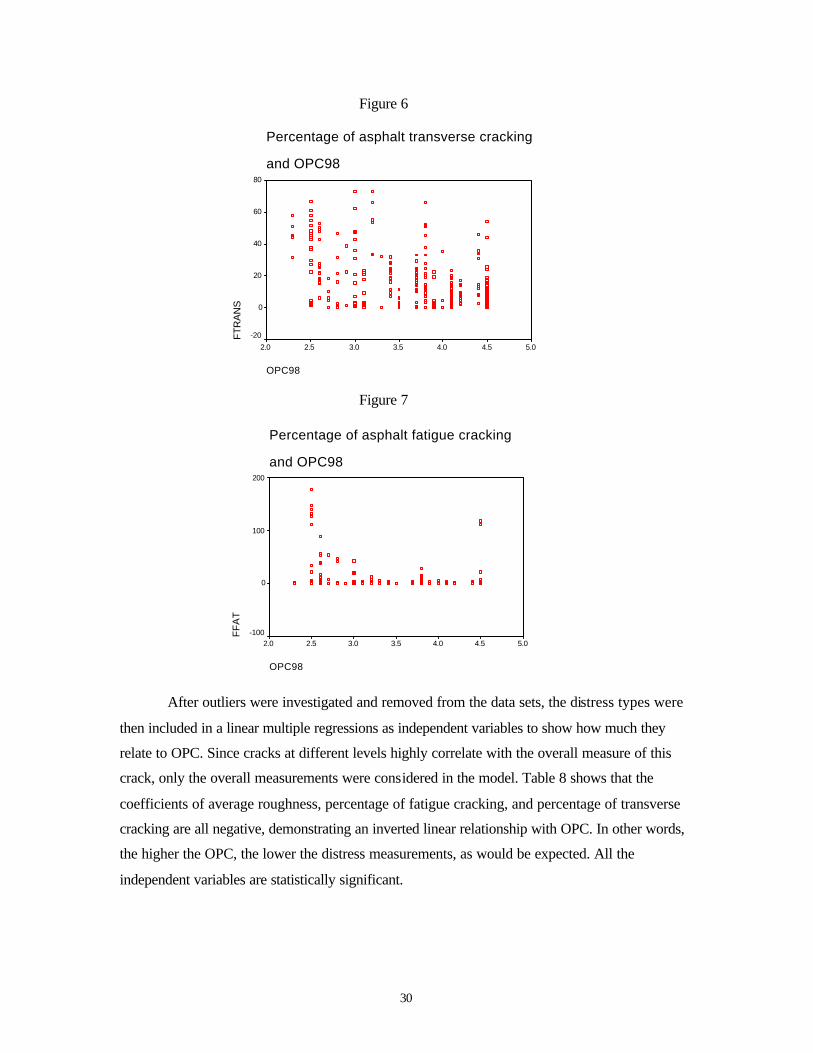
30
Figure 6
Percentage of asphalt transverse cracking
and OPC98
OPC98
5.04.54.03.53.02.52.0
FTR
AN
S
80
60
40
20
0
-20
Figure 7
Percentage of asphalt fatigue cracking
and OPC98
OPC98
5.04.54.03.53.02.52.0
FF
AT
200
100
0
-100
After outliers were investigated and removed from the data sets, the distress types were
then included in a linear multiple regressions as independent variables to show how much they
relate to OPC. Since cracks at different levels highly correlate with the overall measure of this
crack, only the overall measurements were considered in the model. Table 8 shows that the
coefficients of average roughness, percentage of fatigue cracking, and percentage of transverse
cracking are all negative, demonstrating an inverted linear relationship with OPC. In other words,
the higher the OPC, the lower the distress measurements, as would be expected. All the
independent variables are statistically significant.

31
Table 8 Coefficients of Distress Types
Coefficients a
4.360 .076 57.515 .000
-4.2E-03 .002 -.140 -2.400 .017
-3.1E-03 .001 -.220 -4.102 .000
-1.7E-02 .003 -.396 -6.749 .000
(Constant)percentage of fatiguecrackingaverage roughnesspercentage of transversecracking
Model1
B Std. Error
UnstandardizedCoefficients
Beta
Standardized
Coefficients
t Sig.
Dependent Variable: OPC98a.
The correlation of roughness to OPC was also examined. Roughness is determined by response or
profile measure. It can be expressed in several forms. The International Roughness Index (IRI) is
a measure of roughness expressed in inches/miles that can be determined from either method of
measurement and has been recognized by the FHWA. The IRI value has a minimum value of 0
inches/miles and has no maximum value because it is expressed as a measure unit. It is defined,
according to the International Road Roughness Experiment held in Brazil in 1982, as the average
rectified slope of a standard quarter-car simulation traveling 80 kilometers per hour. FHWA has
selected the IRI as the most suitable pavement roughness statistic for incorporating pavement
roughness into the Highway Performance Monitoring System (HPMS) database. Roughness
condition ranges have been suggested by the FHWA to classify the IRI measure into appropriate
condition categories, as shown in the Table 9.
Table 9 IRI and Roughness Category
IRI Range (inches/mile) Roughness Category 0 – 190 Smooth 190 – 320 Medium > 320 Rough
Using a least-square fitness curve to represent the most likely trend of the data points as
shown in figure 8, the relationship between the OPC and roughness figure was revealed as
linearly inverse correlation. There is some indication that as roughness values go beyond 200, an
OPC value of 2.5 can be could be seen as a trigger value to take rehabilitation action.

32
Figure 8 OPC and Roughness
OPC98
Average Roughness
4003002001000
5.0
4.5
4.0
3.5
3.0
2.5
2.0
Observed
Linear
R2 = .27
Another roughness index is the computed Ride Number (RN). The RN is a
ride/roughness statistic with values from 0 to 5 where 5 indicates a very smooth pavement. The
RN uses the form:
RN = ƒ(PI)
PI = ( )[ ] ( )[ ]{ } 5.021
2 PRMSPRMS r +
Where RMS = room mean square of vertical acceleration
rP = measured displacement amplitude of right wheel path for pavement
wavelengths 1.6 ft to 8 ft.
1P = measured displacement amplitude of left wheel path for pavement
wavelength 1.6 ft to 8 ft.
As the higher ride number represents a smoother road, the correlation between ride
number and OPC is expected to be a positive linear relationship. DelDOT's OPC with the ARAN
ride data are plotted in figure 7. A correlation exists but the plot also reveals many variations
within the data points and the curve only explains 20% of the variances.

33
Figure 9 OPC and Ride Number
OPC98
Ride Number
654321
5.0
4.5
4.0
3.5
3.0
2.5
2.0
Observed
Linear
R2 = .20
Analysis described concerning comparison between DelDOT's OPC and automated
distress measures were limited to examining whether there were correlations with particular
distresses and roughness measures. Another approach would be to determine a method of
combining the distress measurements into an overall condition index. In Baladi's study, he
introduces the methods of creating an overall Pavement Quality Index (PQI) or Pavement
Condition Index (PCI) on the basis of individual distress indices. After obtaining Categorized
Evaluation Indices (CEI) such as surface distress index, drainage index, structural index, etc, a
relative weight factor can be assigned to each index category. The PQI or PCI can then be
calculated by summing the products of each CEI and the appropriate weight factor. A threshold
value of the PCI/PQI can be established below which a pavement section is rendered
unacceptable and in need of repair. Because of the difficulty in establishing the proper weights
for each distress, an overall index was not formulated for the DelDOT data.

34
Section Two: Pavement Performance Modeling
Factors Used to Predict Performance
Independent variables used for predicting pavement performance are derived from one or
more of the following factors:
1) Period during which the pavement has been in service
2) Traffic volume and weight, expressed in terms of yearly equivalent single -axle loads
3) Thickness of last overlay, in inches
4) Surface deflection
5) Construction quality
6) Climate factors such as temperature and precipitation
7) Pavement Material Type
8) Drainage
The DelDOT pavement management database is composed of pavement data attributes
covering pavement identification, functional classification, surface type, layer material properties,
and traffic records. Data for two counties, New Castle and Sussex, representing the North District
and the South District, respectively, were available for this study. In the databases, each pavement
attribute or set of related attributes is associated with a variable length segment of pavement by
specifying beginning and ending mile-points. Through discussion with APTech and a review of
the local conditions in Delaware, DelDOT decided to take into consideration the following factors
to predict OPC: age, pavement type, and structure number.
Age
Age is significant because; it is a common factor in the estimation of both cumulative
traffic loads and environmental loads over the life-cycle period; age can be determined for any
pavement and would be expected to be a good predictor; and age can be a surrogate for the
cumulative effect of many detrimental factors, such as thermal effects, subgrade movements,
freeze-thaw effects and bitumen aging. To closely reflect the roads service time on a life-cycle
basis, the age of a road was defined as the number of years since the road was last improved. In
modeling the relationship of age with OPC, the age of the road segment at the time that the OPC

35
rating was taken was used.
Pavement Type
Pavement material type is also critical to pavement performance. The preliminary
investigation of the data from the South District resulted in the groupings of 23 different
pavement families based on surface type. Among these 23 families, only five families contained
enough data to conduct regression analysis using pavement type. Therefore, the data was then
regrouped into more general families --- rigid, composite, flexible, surface treatment,
unimproved, and unconventional. Surface treatments were excluded from the modeling because
their rehabilitation needs are determined on a cyclic basis, rather than on conditions. Unimproved
and unconventional types --- including graded and drained, soil, grave, stone, bricked, and other
combinations were not considered in the study. The distribution of the data for each family is
shown in Table 10. The groupings of the many surface types that exist for Delaware roads into
the above families are listed in detail in Appendix D.
Table 10 Family Distributions
family classfication
1194 12.5 12.5 12.53418 35.7 35.7 48.13175 33.1 33.1 81.31615 16.9 16.9 98.1
131 1.4 1.4 99.536 .4 .4 99.914 .1 .1 100.0
9583 100.0 100.0
rigidcompositeflexiblesurface treatmentunimprovedunconventionalunknownTotal
ValidFrequency Percent
ValidPercent
CumulativePercent
Structure Number
For flexible pavements, the structure number is expressed by the thickness of each of the
pavement layers through the use of layer coefficients as given by:

36
SN = a1D1 + a2D2 + a3D3
Where: SN = structural number representing the structural capacity of the
pavement; D1, D2, D3 = layer thickness; a1, a2, a3 = layer coefficients
The layer coefficients are empirical parameters relating the layer thickness to the structural
number and expressing the relative ability of a material to function as a structural component of
the pavement. Theoretical layer coefficients for any material can be developed using multi-layer
elastic analysis and comparing strain and stress levels within the pavement layer structure.
Materials that are not assigned AASHTO coefficients are assigned a structural number based on
coefficients (recommended by Materials and Research) multiplied by the thickness of the
pavement layers.
According to AASHTO road tests, the road structure, as indicated by the structure
number, influences the deterioration of flexible pavements with and without overlay. Composite
and overlaid pavement equations include asphalt surface thicknesses as well. Structure number is
believed to be an indicator of mechanistic parameters of how a pavement performance is effected
by stress, strain, and deflection. Theoretically, a pavement with better materials has a higher
structural number than a pavement with less resilient materials. Similarly, if two pavements are
made with the same materials, a thicker pavement would have a higher structural number than a
thinner pavement. Structure number is also used when designing pavements to meet expected
loads and usage.
Model Procedure
Groupings of Highway Sections
Many factors may influence pavement performance and each has a distinctive effect over
time. Ideally, a pavement model could be constructed to reflect the unique characteristics of each
road. However, developing performance models for each road section requires extensive
historical databases and therefore in practice proves to be very difficult. Instead, a method of
categorizing pavements based on similar characteristics is often chosen to account for the wide
variety of factors on a network-level basis, assuming that pavements with the same grouping will
perform similarly throughout their lives.
37
Early in the research, data for roads were studied in 23 groupings corresponding to
various pavement types. Further detail was introduced by looking at different functional
classifications of roads within pavement types. Because of sparse data in many of the groups, and
because of the great variation in the data for OPC and age (see ApTech Phase I report), a more
general grouping was selected. Pavement sections with similar characteristics were finally
grouped into three families, rigid, composite, and flexible, and the development of performance
models was focused on each of these groups.
Screening Procedure
Errors were identified as those pieces of data in which a mistake was suspected when
gathering, coding, or entering the data. Inaccurate data can be found where basic system rules are
broken. One example is where OPC values are greater than 5 when the OPC scale is from 0 to 5.
The data was sorted by group, time since pavement was built or last rehabilitated, and OPC. For
each family type, scatter-plots were run to display the data distribution between OPC and age.
Obvious problems such as OPC greater than 5 or less than 0, or remaining life less than or equal
to 1 and OPC greater than 4, were eliminated from the database. However, to ensure appropriate
model building, further examination of the data for any unusual observations was performed.
Unusual data values can have substantial impact on model development. To identify
these extreme cases, the deviations from predicted values of OPC were subjected to residual
analysis. Residuals are calculated as the difference between the observed value and the value
predicted by a linear regression model. If the observations are normally distributed about the
regression equation with constant variance, then the residuals should be approximately normally
distributed. To check this, histograms of residuals were plotted (figure 10 shows an example). A
normal plot of residuals should approximate a bell shape about 0. The standard deviation of the
residuals is used as a measure of spread to observe the relative magnitude of any particular
residual. If an observation has a residual that is several standard deviations below or above 0, it is
an outlier and should be checked. The probability that a deviation in either direction will exceed
three standard deviations is close to zero. Therefore, any deviation larger than three standard
deviations was assumed to be out of the expected values and the case was listed as an outlier (see
Table 11 for an example).

38
Figure 10 Histogram of Residual
Regression Standardized Residual
4.003.50
3.002.50
2.001.50
1.00.500.00
-.50-1.00
-1.50-2.00
-2.50-3.00
-3.50-4.00
-4.50-5.00
Histogram
Dependent Variable: OPC96
Fre
quen
cy
1000
800
600
400
200
0
Std. Dev = 1.00
Mean = 0.00
N = 3237.00
Table 11 Sample Outliers
Casewise Diagnosticsa
-3.391 1.50 3.3685 -1.8685-4.844 1.00 3.6690 -2.6690-3.066 2.10 3.7893 -1.6893-3.247 2.00 3.7893 -1.78933.834 5.00 2.8876 2.11243.943 5.00 2.8275 2.17253.943 5.00 2.8275 2.17253.943 5.00 2.8275 2.17253.943 5.00 2.8275 2.17253.943 5.00 2.8275 2.1725
-3.247 2.00 3.7893 -1.7893-3.247 2.00 3.7893 -1.7893-3.247 2.00 3.7893 -1.7893
Case Number148104811633974650365046505650665076508779677977798
Std.Residual OPC96
PredictedValue Residual
Dependent Variable: OPC96a.
Linear Regression Analysis
After errors and outliers were eliminated from the data file, the first method used in
developing prediction curves was a linear regression analysis. This method used age as a single
independent variable (suggested by DELDOT and ApTech as a first approach) in making the

39
prediction. The data plots in figure 11, 12 and 13 show the data points and the linear model.
Linear models for rigid, composite, and flexible models explain only about 17%, 27%, and 19%,
respectively, of the variance. For any given age there is a wide range of OPC values. The data
plots of the flexible family and the composite family distribute in a visible square shape that
contains unexpected relationships of low age with low OPC and high age with high OPC. The
slope of the regression lines indicates a slower decrease in OPC with age than would be expected.
The flatter slope is expected with data that has such variability. Also the intercepts at Age = 0
indicate an OPC less than 4.0 which does not correspond to the definition of OPC where OPC = 5
for a new road. Therefore, the linear models for the three families were not satisfactory.
Figure 11 Linear Model for Rigid Family
OPC96
age
3020100
5.5
5.0
4.5
4.0
3.5
3.0
2.5
2.0
1.5
Observed
Linear
R2 = .17
Figure 12 Linear Model for Composite Family
OPC96
age
3020100
5.5
5.0
4.5
4.0
3.5
3.0
2.5
2.0
1.5
Observed
Linear
R2 = .27

40
Figure 13 Linear Model for Flexible Family
OPC96
age
3020100
6
5
4
3
2
1
Observed
Linear
R2 = .19 Non-linear Regression Analysis
One of the assumptions of pavement performance modeling is that a section of pavement
deteriorates with time at different rates during the life of the pavement; therefore, an appropriate
model would be a curvilinear relationship between OPC and age. In Nunez and Shahin's study in
1986, a third-order polynomial regression model was successfully developed to predict the
pavement condition when a single condition indicator was used. The study concluded that
pavement condition forecasting could be accomplished by customizing the prediction for each
individual road section depending on its condition in relation to the prediction model curve for
the pavement family. A typical performance curve is shown in Figure 14. In this model, to predict
the future pavement condition, the model curve is translated to pass through the present PCI-AGE
point, which is parallel to the prediction model curve for the pavement family. The PCI can then
be determined at the desired future AGE by reading from the adjusted curve. A similar model was
used in the DelDOT project with PCI/LAW.
Pavement performance models already developed from other sources revealed that the
equations developed as a result of this model take the form of the constrained least-square
equation:
OPC = +0p xxxpxxpxp ****** 321 ++
where x is the age, p0, p1, p2, and p3 are the coefficients

41
Figure 14 Pavement Condition Forecasting Model
Two approaches were used to model non-linearity. In the first of these, a cubic function, a
curvilinear function having two bends was used to find the best-fit curve. The second approach
used a mathematical transformation of the age variable into square and cubic terms such that each
of these three variables is linearly related to the dependent variables. The second approach is
helpful in finding the intercept and coefficients.
Table12 Statistical Parameters of First-order Linear Prediction Models
(South and North districts)
Type of Pavement Regression Coefficient R2
Rigid
P0 = 3.615 P1 = 0.0345
0.17
Composite
P0 = 3.813 P1 = 0.0633
0.27
Flexible P0 = 3.722 P1 = 0.0564 0.18
Pavement Condition Index
Time in Years
Pavement Family Prediction Model
Present PCI-AGE
Modified Prediction Curve

42
Table13 Statistical Parameters of Third-order Polynomial Prediction Models (South and
North)
Type of Pavement Regression Coefficients R2 Rigid P0 = 4.077
P1 = -0.290 P2 = 0.029 P3 = -0.0009
0.30
Composite P0 = 4.053 P1 = -0.224 P2 = 0.0018 P3 = -0.0005
0.35
Flexible P0 = 4.013 P1 = -0.211 P2 = 0.018 P3 = -0.0006
0.23
Non-linear models were plotted as shown in figures 15 through 22, to reflect the
relationship between OPC and age for the three families in the North Districts, South Districts
and the pooled data combining the North and the South. Comparing third-order polynomial
models with first-order linear models as shown in Table 12 and Table 13, the prediction models
of third-order polynomial fit better than linear models in terms of intercepts, slope and R2 values.
For all three families, nonlinear models explain significantly more variance than do linear
models. Nonlinear models also show a varying rate of deterioration along the life of the
pavements with a negative slope as the start, a positive slope next, and larger negative slope in the
end. However, the nonlinear models still have difficulties in reflecting the expected degradation
of the road surface, compared with theoretical models. The intercepts for the three families were
all around an OPC of 4. At age = 0, when a road is new or newly rehabilitated, an OPC of at least
4.5 is expected. Also the slopes prove to be very flat with OPC values fluctuating around 2 to 4.
It is obvious in looking at the figures that these models perform poorly in modeling the
performance of the roads. There are features in the data that limit the types of models that can be
generated and the degree to which the physical realities will be reflected. Most notably are
portions of the curve at about the 10-year range that would indicate improving road condition
with age as the slope of the curve becomes positive. One explanation of the problem might be that
by the time most roads reach this age they have reached a condition that warrants rehabilitation.
The data points that are left are those roads that for some reason are in better condition at higher
age, therefore distorting any models generated from the data. There is a general problem at
higher age values of a lack of data, and a lack of representative data. There is also a problem of a

43
low number of high values for OPC (4.5 to 5) for low age, forcing a low intercept.
Another factor affecting the fitness of the model is the scale of OPC. The use of the 0-to-
5 scale, in addition to the fact that the evaluation of OPC is subjective, restricts the raters' ability
to provide a comprehensive and accurate reflection of the real road condition. The range of OPC
as reflected in the data is really from 2.0 to 5.0. With such a small range, high variability, and
obvious problems with the data particularly for the high age portions, the ability to formulate
realistic models is impossible.
Figure 15 Rigid Families in the North District
OPC 96
AGE96
20100
6
5
4
3
2
1
Observed
Cubic
Figure 16 Composite Families in the North District
OPC 96
AGE96
20100
6
5
4
3
2
1
Observed
Cubic

44
Figure 17 Flexible Families in the North District
OPC 96
AGE96
3020100
6
5
4
3
2
1
Observed
Cubic
Figure 18 Composite Families in the South District
OPC_96
OPC96AGE
20100
5.5
5.0
4.5
4.0
3.5
3.0
2.5
2.0
1.5
Observed
Predicted
Figure 19 Flexible Families in the South District
OPC_96
OPC96AGE
20100
6
5
4
3
2
1
0
Observed
Predicted

45
Figure 20 Rigid Families in pooled data
OPC96
age
3020100-10
5.5
5.0
4.5
4.0
3.5
3.0
2.5
2.0
1.5
Observed
Cubic
Figure 21 Composite families in pooled data
OPC_96
OPC96AGE
20100
5.5
5.0
4.5
4.0
3.5
3.0
2.5
2.0
1.5
Observed
Predicted
Figure 22 Flexible families in pooled data
OPC_96
OPC96AGE
20100
6
5
4
3
2
1
0
Observed
Predicted
46
Inclusion of Structure Number
Structure number was included in the linear models of OPC and age. Roads were viewed
in the three families; Rigid, Composite, and Flexible. Linear models for the three pavement types
addressed were determined to be:
Rigid
OPC = 2.124 + .159 * S - .015 * A
Composite
OPC = 3.99 - .04 * S - .075 * A
Flexible
OPC = 3.77 + .094 * S - .066 * A
Where S = structure number, A = age
Differences were evident between the three pavement families. With rigid pavements the
age variable is weak with structure strong. For composite pavements structure is weak and the age
effect much stronger. Composite and flexible pavements are similar for aging but very different
with respect to structure. While the models showed significant effects of both age and structure
number, this method was believed to be inappropriate because: (1) The equations reflect that
thicker pavements are in better condition than thin pavements, even at an age of zero. This
contradicts with the principle that the highest rating (in this case a 5) reflects the condition of a
pavement in its initial construction state. (2) Since the structural number does not change over
time unless rehabilitation is applied, the model is only reflecting the deterioration of the OPC due
to age, while restricting the highest possible OPC for a pavement at age zero based on its
structure number.
In order to test the effects of structure number, the model was then revised to take the
structure number out of the equation and instead, use it to further divide the pavement family.
Pavements were grouped by surface type, and these families were further divided into categories
based on structure numbers with at least two categories defined to represent strong/weak or
thick/thin pavements. Data from the North District did not include structure number, so only the
South District data was examined in this manner.
A cross tabulation of structure number with pavement type (See Appendix D) indicates

47
the correlation of structure number with the three surface type families. Because the road sections
clustered around several structural numbers, each of which has a number of observations less than
50, the production of any reasonable model classified by different groups of structure numbers
was not possible. It was recognizable, however, that a structure number of 6.4 is a dividing line
between the composite family and flexible family. Anything below 6.4 in the composite family
was treated as outliers and thus was not included in the modeling.
In order to test the hypothesis that family categorization by structure number contributes
to different models and thereby should be individually treated based on family, two dummy
variables were created in a third-order polynomial regression model shown below:
Table 14 Dummy Variables for Family Classification
S1 S2 Flexible (sn=0~6.4) 1 0 Composite (sn=6.4~10.2)
0 1
Composite (sn=10.2~20.6)
0 0
In the model, the base group for comparison was the one where S1 = 0 and S2 = 0, that is,
structure number falls in the category 10.6 ~ 20.6. S1 group represents flexible, and S2 group
represents composite with structure numbers from 6.4 to 10.2.
The data tested was from the South District with OPC98 as the dependent variable.
OPC98 was believed to be the most reliable reflector of the road conditions in the three indices.
The following is the statistics summary.

48
Table 15 Model Summary of Family Testing
Model Summary
.527a .278 .275 .5900013Model1
R R SquareAdjusted R
Square
Std. Errorof the
Estimate
Predictors: (Constant), S2XC, S1XC, S2, OPC98AGE,S1, S2X, S1X, AGE98S, AGE98C, S1XS, S2XS
a.
Table 16 Coefficients of Family Testing
Coefficients a
4.415 .110 40.206 .000-.226 .053 -1.614 -4.241 .000
1.46E-02 .007 2.167 2.100 .036-4.4E-04 .000 -1.549 -1.778 .076
-.376 .124 -.271 -3.021 .0033.85E-02 .121 .027 .318 .750
.153 .057 1.101 2.689 .007-1.4E-02 .007 -1.602 -2.012 .044
4.61E-04 .000 1.029 1.822 .069-1.2E-02 .056 -.087 -.221 .825-5.5E-04 .007 -.066 -.077 .938
1.75E-04 .000 .492 .694 .488
(Constant)OPC98AGEAGE98SAGE98CS1S2S1XS1XSS1XCS2XS2XSS2XC
Model1
B Std. Error
UnstandardizedCoefficients
Beta
Standardized
Coefficients
t Sig.
Dependent Variable: OPC_98a.
The final equation from the above model was:
Y = 4.415 - 0.226x + 0.014x2 - 0.004x3 - 0.376S1 + 0.153S1x - 0.014S1x2 +
0.0005S1x3 + 0.038S2 - 0.012S2x - 0.0005S2x2 + 0.0002S2x3
Where Y represents OPC, x is age.
Note that in the Table 17, all the t statistics of coefficients in the S2 group (composite
family with structure numbers from 6.4 to 10.2) are not significant and those of S1 group (flexible
family) are significant. It signifies that the inclusion of flexible family into a composite-based
model does make a difference.

49
The next step was to test if division of structure number within one family makes a
difference. In order to do that, a dummy variable, c was created. When c = 0, it represents thin
pavements whose structure numbers are from 6.4 to 10.2; when c = 1, it represents thick
pavements whose structure numbers are from 10.2 to 14. Remember structure numbers greater
than 6.4 are considered as composite family.
The modeled equation with dependent variable OPC98 is:
OPC98 = 4.436 - 0.230*age + 0.014*age2 - 0.0003*age3 + 0.079*c +
0.024*c*age - 0.009*c*age2 + 0.0003*c*age3
Major statistics summary was also generated:
Table 17 Model Summary of Structure Number Testing
Model Summaryb
.664a .441 .438 .5004864Model1
R R SquareAdjusted R
Square
Std. Errorof the
Estimate
Predictors: (Constant), CXC, OPC98AGE, C,AGE98C, CX, AGE98S, CXS
a.
Dependent Variable: OPC_98b.
Table 18 Analysis of Variance of Structure Number Testing
ANOVAb
280.714 7 40.102 160.096 .000a
356.443 1423 .250637.157 1430
RegressionResidualTotal
Model1
Sum ofSquares df
MeanSquare F Sig.
Predictors: (Constant), CXC, OPC98AGE, C, AGE98C, CX, AGE98S, CXSa.
Dependent Variable: OPC_98b.

50
Table 19 Coefficients of Structure Number Testing
Coefficientsa
4.436 .054 81.901 .000-.230 .023 -1.691 -9.896 .000
1.43E-02 .003 1.908 5.324 .000-3.2E-04 .000 -.747 -3.534 .0007.89E-02 .088 .055 .900 .3682.38E-02 .043 .133 .550 .583-9.1E-03 .006 -.666 -1.587 .1133.12E-04 .000 .359 1.496 .135
(Constant)OPC98AGEAGE98SAGE98CCCXCXSCXC
Model1
B Std. Error
UnstandardizedCoefficients
Beta
Standardized
Coefficients
t Sig.
Dependent Variable: OPC_98a.
Note that the t statistics of variables c, cx, cxs and cxc are not significant. This means that
our breakdown of structure number into thin pavements and thick pavements does not make a
statistical difference. An identical investigation into flexible family, as shown below, discovers
that by dividing the family into two separate groups, 0.5~1.5 and 1.5~6, the t statistics of those
independent variables relating to the dummy variable B, which is composed of the classification
of the two groups, are also not significant (the significant levels are larger than .05).
Table 20 Coefficients Statistics of Flexible Family
Coefficients a
4.211 .102 41.209 .000-.172 .048 -1.072 -3.595 .000
1.23E-02 .006 1.380 2.009 .045-3.9E-04 .000 -.733 -1.756 .079
.199 .186 .137 1.072 .284-5.8E-02 .081 -.345 -.719 .4729.33E-03 .010 .701 .925 .355-4.0E-04 .000 -.451 -1.114 .266
(Constant)OPC98AGEAGE98SAGE98CBBXBXSBXC
Model1
B Std. Error
UnstandardizedCoefficients
Beta
Standardized
Coefficients
t Sig.
Dependent Variable: OPC_98a.
Within one district, the families divided by surface types seem to show statistical
difference between each other, whereas the effects of further division by structure number within

51
individual families are minimized. Therefore, the deterioration pattern seems to be affected by
contributions of different material types. The results of this analysis indicated that grouping roads
by ranges of structure number (generally thick and thin pavements) offered no statistical
significant improvement in models.
Improvements on Pavement Management Databases
The availability of a reliable pavement management database is the foundation of any
pavement management system and any attempts at performance modeling. Throughout the
project, the DELDOT Pavement Management Team worked to put together pavement history
data on age and structure of roads through a detailed and often difficult review of hard copy
project files in DELDOT archives. For the first time, a pavement history database was developed
for all roads maintained by DELDOT for all counties. The data includes original construction
information, materials, dates and details of follow-on rehabilitation. A number of corrections and
refinements to the data were made during the course of the project. The DELDOT Pavement
Management Team has been active in department wide efforts to better coordinate and improves
data collection efforts.
Previous pavement management initiatives at DelDOT in the early 1990's suffered for a lack of
data. Also, while previous computer software was well grounded in current theory, DELDOT
personnel had difficulty in updating and working with road databases. Since then a number of
personal computer based tools for managing data have become available such as Microsoft
Access and Microsoft Excel. DELDOT Pavement Management personnel feel comfortable
working with such tools and are enthusiastic about having more capabilities of constructing and
analyzing their data. With some assistance from CADSR, they initiated the creation of a
Microsoft Access application to capture information from their rehabilitation projects.

52
Part III, Section Three, Summary of Findings
The work done by the Center for Applied Demography and Survey (CADSR), through
the Delaware Transportation Institute, in support of DELDOT's 1997 Pavement Management
System (PMS) Enhancements was focused on the following tasks.
• A review of current practices in pavement management systems.
• A review of data needed for PMS and availability of data at DELDOT.
• Evaluating the current OPC and how it relates to road degradation through the life of the
roads.
• Assistance in examining how the current OPC could be used in the construction of road
performance models.
What follows is a summary of findings related to these tasks.
A review of current practices
A number of the State initiatives have demonstrated the success and importance to
pavement management of providing information on the current and future state of pavement
conditions, and systematic procedures for evaluating rehabilitation options while taking into
account as much as possible the relative economic advantages and disadvantages. PMS assists
with the technical problems of choosing optimal times, places, and techniques for repairing
pavements and simultaneously, providing those in charge of maintaining and improving roads
with the data and other technical justifications needed to secure political support for adequate
road maintenance. These agencies employed different methods to improve the way they manage
their pavements, but they all experienced a similar outcome. Because of their pavement
conditions surveys and data analysis schemes, they were able to produce better-maintained
pavements from available resources and ensure more effective technical input into the political
decision-making process.
Perhaps the most relevant research toward defining the components of a pavement
management system was conducted by OECD (Organization of Economic and Cooperative
Development) Expert Group that suggests that the pavement maintenance procedure consists of
four steps.

53
• Data collection
• Models/analysis
• Criteria /optimization
• Consequences/implementation
AASHTO guidelines suggest seven conditions necessary for the development,
implementation, and operation of a PMS.
• Strong commitment from top management and coordination throughout the department.
• A steering committee that exclusively deals with organizational and political problems.
• PMS Staff including one person should be the lead PMS engineer with full time responsibility for managing, coordinating, and operating the PMS.
• System selection or development including good data, good analysis, and effective communications.
• Demonstration of PMS on a limited scale.
• Full-scale implementation – The pavement management team established earlier is very important to successful implementation.
• Periodical review and feedback.
In regards to the development of pavement performance models, promising work by
Nunez and Shahin in 1986 provides an example and demonstration of the application of a third-
order polynomial regression model to predict the pavement condition. The suggested model
relates well to what is known about the pattern of degradation of roadways, and the study
suggested methods of adapting a network level model to the prediction of a particular road's
performance.
A review of data needed for PMS and its availability
The literature suggests the following types of data to be used as predictors for pavement
management systems:
• Pavement condition measures
• Surface distress measures
• Period during which the pavement has been in service (age, time since last rehabilitation)

54
• Traffic volume and weight, expressed in terms of yearly equivalent single -axle loads
• Thickness of last overlay, in inches
• Surface deflection
• Construction quality
• Climate factors such as temperature and precipitation
• Pavement Material Type(s) and thickness of layers
• Drainage
DELDOT is in the process of constructing a pavement history database for all State
maintained roads in Delaware. The data includes the pavement age or last date of rehabilitation,
OPC measures, and the material type(s) and thickness(s) that make up each road. DELDOT
Pavement Management Team made considerable efforts over the last year to compile this
information from hard copy as-built records and contracts in DELDOT archives. They have
initiated procedures and built computer-based tools to maintain the data. Accurate and current
data are crucial to any type of multi-year prioritization of pavement projects and these efforts
have yielded considerable progress over past efforts. Efforts should also be made to include
traffic volume and traffic weight (ESALs) in the database. As the database is continually refined
and maintained, its value will increase in its ability to support a better understanding of the
current and future condition of roads. Eventually given improved pavement condition data a
history of individual road performance over several years will be available. At this point, overall
pavement condition ratings are only available for 1996, 1997, and 1998.
It is recommended that the data go through continual review and quality control with
particular emphasis on understanding why many roads have low OPC values with low age, and
why there numerous roads that have high OPC values with high age (greater than 10 to 15 years).
Evaluating the current OPC and how it relates to age
The following points summarize the evaluation of the OPC rating used at DelDOT and its
relationship to age.
• OPC is a subjective measure for the upper end of the five-point scale and for this portion of
the scale is based on examining the extent of four surface distresses.
• Roads that are within 5 years of needed rehabilitation are assigned OPC values by referencing

55
a fixed table for each pavement type. OPC then is constrained to a fixed relationship with
age and directly related with a subjective estimate of remaining life.
• OPC results from two very different subjective rating methods.
• OPC values generally are assigned to half points of the scale, i.e. 2.5, 3.0, 3.5, 4.0, 4.5,
indicating that OPC is not a true continuous variable and takes on a limited set of values
owing to the raters difficulty in quantifying in more detail the overall condition of roads.
• Plots of OPC versus age show trends of decreasing OPC with increasing age but there does
not appear to be a systematic relationship that would be indicated by what is known about the
degradation of pavements. In an examination of OPC as it relates to the time a road was last
rehabilitated (age), there exists great variability in the values of OPC at a given age. Values
of OPC less that three are common even after a few years since rehabilitation. OPC values of
5 are found even after 10 years of pavement life. These "low age - low OPC" and "high age
- high OPC" data points would seem to signal problems with the data, and at a minimum
suggest the need for a closer look at the data to find an explanation.
• Statistical analysis indicates a significant difference in the OPC measures for 1996, 1997, and
1998. The 1998 survey has the best fit with 3rd order polynomial models using age as the
independent variable. This would support the DelDOT Pavement Management Team's
statement that each year OPC ratings were more reliable and were subject to more quality
control.
• OPC is correlated with measures taken by automated means for individual surface distress
measurements that included transverse cracking, fatigue cracking, the International
Roughness Index (IRI) and Ride Number. As OPC is an overall condition index, it would be
necessary to develop methods to combine individual automated surface distress
measurements into an overall surface distress index for the purpose of further examining the
validity of the OPC rating. Many of the difficulties in modeling the performance of roads in
Delaware are attributable to the lack of an objective measure of pavement condition. CADSR
concurs with APTech Inc.'s recommendation that DELDOT determine whether distress
information obtained by automated means would be sufficient to develop a new OPC rating
that would be objective and more comprehensive.
The development of pavement performance models
Data within the DelDOT Pavement History databases was used to develop performance
models. DelDOT OPC rating for the years 1996, 1997, and 1998 provided data for the dependent

56
variable, and age, pavement type, structure number were the factors investigated as independent
variables. The analysis can be summarized as follows.
• As the DelDOT Pavement Management team is focused on the network level, and because of
the lack of historical data on pavement condition, it is appropriate to develop models for
groupings of roads rather than addressing roads individually. The initial attempt at dividing
roads into 23 families by pavement type was not effective in that there was minimal data for
all but 6 of these families and because of the great variation of OPC for any given age. When
roads were grouped into the three families; Flexible, Rigid, and Composite, the modeling was
simplified. Statistical analysis indicated that pavement performance models of these three
families were significantly different from each other.
• The high variation of OPC for a given age, the limited scale of OPC, the low values of OPC
with low age, data gaps, and questionable data at age greater than about 10 years, all
contribute to unsatisfactory, inapplicable performance models.
• 3rd order polynomial models are indicated as the most likely form for performance models
rather than linear or other forms. Even with polynomial models that would best correspond
to the expected pattern of degradation of roadways, the deficiency in the available data and
the problems with the subjective measure of OPC result in models that can not be used to
support multi-year prioritization of projects or preventive maintenance forecasting.
• Analysis indicated that grouping roads by ranges of structure number offered no statistically
significant improvement over grouping by Composite, Flexible, and Rigid types.

57
BIBLIOGRAPHY AASHTO, Guidelines for Pavement Management Systems. Washington, D.C., 1990 Amekudzi, Adjo A. and Attoh-okine, N.O. “Institutional Issues in Implementation of
Pavement Management Systems by Local Agencies” TRB1524 pg. 10, 1994 Applied Pavement Technology, Inc., Delaware Department of Transportation (DelDOT)
Pavement Management Systems Enhancements, Phase I report. 1997 Baladi, Gilbert and Snyder, Mark, Highway Pavements Training Course (Memo),
Department of Civil Engineering, Michigan State University, 1998 Byrd, L.G., NCHRP Synthesis of Highway Practice 58: Consequences of Defferred
Maintenance, Transportation Research Board, National Research Coucil, Washington, DC, 1979
Carmines, Edward G. and Zeller, Richard A., Reliability and Validity Assessment, Sage Publications, Beverly Hills, California, 1979 Federal Aid Highway Program Manual, Transmittal 428, Vol 6, Ch. 2, Sec. 4, SubSec. 1.
FHWA, U.S. Department of Transportation, March 1989 Geoffroy, Donald N., NCHRP Synthesis of Highway Practice 223: Cost-Effective
Preventive Pavement Maintenance. Transportation Research Board, National Academy Press, Washington, D.C. 1996
George, K. P. and Rajagopal, A. S. and Lim, L. K., “Models for Predicting Pavement
Deterioration”, TRB research Records No.1215, Papers for 68th annual meeting of the Transportation Research Board, 1989
Hass, R. and Hudson, W. R., Pavement Management Systems. McGraw-Hill, Inc., New
York, N.Y., 1978 Irrgang, Federico C. and Maze, T.H., “Status of Pavement Management Systems and
Data Analysis Models at Sate Highway Agencies”. TRB Research Record No. 1397. National Academy Press, Washington D.C. 1993
Johnson, K. D. and Cation, K.A., Performance Prediction Development Using Three
Indexes for North Dakota Pavement Management Systems. In Transportation Research Record 1344, TRB, National Research Council, Washington, D.C., 1992, pp.22-30
Kohn, O’Brien and Shahin, “Prediction of Pavement Performance by Using
Nondestructive Test Results”. Transportation Research Record 943, TRB, National Research Council, Washington, D.C., 1983, pp. 13-17

58
Martin, James, The Data-Base Environment, Prentice-Hall, Inc., Englewood Cliffs, New
Jersey. 1983 Nunez, Maria Margarita and Shahin, Mohanmed Y., “Pavement Condition Data Analysis
and Modeling”, TRB research Records No.1070, National Transportation Council, Washington D.C. 1986
OECD Expert Group, “Pavement Management Systems”, OECD Road Transportation
Research, Systems DE Gestion, Paris, France, 1987 PCS/LAW Engineering Report Pavement Management Systems for the State of
Delaware, 1990 Smith, Harry A. and Stephands, Peter J. etc. “Development of Delaware Department of
Transportation Pavement Management Systems” TRB 1397 pg 54
Smith, R. E. Addressing institutional Barriers to Implementing a PMS, Pavement
Management Implementation (F.B. Holt and W. L. Gramling, eds), ASTM, Philadelphia, Pa., 1992
Smith, R. E. and Freeman, Thomas J., “Contracting For Pavement Distress Data
Collection”, 77th Annual Meeting, TRB, Washington D.C. 1998 Strategic Highway Research Program, Distress Identification Manual for the Long-Term
Pavement Performance Project, National Research Council, Washington D.C. 1993
Ullidtz, Per, Pavement Analysis. Elsevier Science Publishers B.V., Amsterdam, Netherlands., 1987
Wang, Kelvin C.P., “Automated Systems for Pavement Surface Distress Survey: A
Historical Perspective on Design and Implementation”, 77th Annual Meeting, TRB, Washington D.C. 1998
Zimmerman, Kathryn A. Cation P.E. “Applying PMS Lessons to New Infrastructure
Tools”, Infrastructure---Planning and Management ed. Jonathan Lgifford, Donald R. Uzarski and Sue McNeil American Society of Civil Engineering 1993
59
Appendix A Correlation of OPC with Distress Types (Asphalt Pavements)
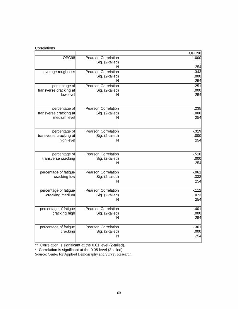
60
Correlations
OPC98OPC98 Pearson Correlation
Sig. (2-tailed)N
1.000.
254average roughness Pearson Correlation
Sig. (2-tailed)N
-.343.000254
percentage of transverse cracking at
low level
Pearson CorrelationSig. (2-tailed)
N
.251
.000254
percentage of transverse cracking at
medium level
Pearson CorrelationSig. (2-tailed)
N
.235
.000254
percentage of transverse cracking at
high level
Pearson CorrelationSig. (2-tailed)
N
-.319.000254
percentage of transverse cracking
Pearson CorrelationSig. (2-tailed)
N
-.510.000254
percentage of fatigue cracking low
Pearson CorrelationSig. (2-tailed)
N
-.061.332254
percentage of fatigue cracking medium
Pearson CorrelationSig. (2-tailed)
N
-.112.073254
percentage of fatigue cracking high
Pearson CorrelationSig. (2-tailed)
N
-.401.000254
percentage of fatigue cracking
Pearson CorrelationSig. (2-tailed)
N
-.361.000254
** Correlation is significant at the 0.01 level (2-tailed). * Correlation is significant at the 0.05 level (2-tailed). Source: Center for Applied Demography and Survey Research

61
Appendix B
OPC Rating Guides
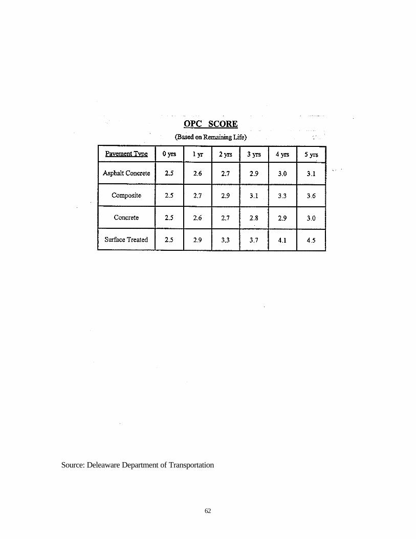
62
Source: Deleaware Department of Transportation

63
Source: Delaware Department of Transportation

64
Source: Delaware Department of Transportation

65
Source: Delaware Department of Transportation

66
Source: Delaware Department of Transportation

67
Source: Delaware Department of Transportation

68
Source: Delaware Department of Transportation

69
Appendix C
Correlation of Pavement Family with Surface Type

70
Correlation of Family with Surface Type

71
surface type * family classfication Crosstabulation
Count
3
128
1555
22
10
46
9
226
719
1662
392
42
3418
1221194
4
10
5
2
1194 3418 3175 1615 131 36
graded anddrained/unimprovedsoil surface graded anddrained/unimprovedsurface treatmentsurface treatment on hotmix on surface/unconventionalsurface treatment on hotmix on soil cementbas/unconventionsurface treatment on soilcementlow type bituminous/surface treatmenthot mix on soilsurface/flexiblehot mix on waterboundbase of stone/flexiblehot mix on surfacetreatment/flexiblehot mix on low typebituminous or sandasphalt/flexiblehot mix on soil cementbase/flexiblehot mix onconcrete/compositehot mix on brickunknownsurface treatment onconcrete/unconventionalhow mix on surfacetreatment/flexibleconcrete alongsidesurface treatment/surfacetreatmentconcrete alongside hotmix/flexible
surfacetype
Total
rigid composite flexiblesurfacetreatment unimproved
unconventional
family classfication

72
APPENDIX D
Crosstabulation of Structure Number and Pavement Type

73
Crosstabulation of Structure Number and Pavement Type
STRUCTUR * 1= rigid, 2= composite, 3= flexible Crosstabulation
Count
1= rigid, 2= composite, 3= flexible
Total
1 2 3STRUCT
UR.00000 1 30 31
.32000 3 3
.40000 1 1
.60000 16 16
.66000 2 2
.80000 10 256 266
.90000 10 101.00000 12 121.06000 1 11.20000 18 566 5841.26000 7 71.30000 3 31.40000 5 51.46000 9 15 241.48000 4 41.60000 95 951.80000 1 11.86000 12 121.90000 3 32.00000 5 32 372.02000 1 12.04000 13 132.10000 9 92.26000 9 92.40000 1 36 372.44000 5 52.48000 14 142.56000 7 72.62000 8 82.66000 18 182.80000 21 212.84000 4 43.04000 1 13.06000 6 63.20000 6 63.24000 4 43.52000 35 353.60000 1 1

74
3.68000 8 83.76000 10 103.92000 13 134.00000 13 134.08000 9 94.24000 32 324.32000 4 44.44000 12 124.56000 1 14.64000 10 104.88000 7 75.12000 14 145.20000 1 15.64000 2 25.68000 29 295.76000 1 16.40000 8 86.80000 1 17.00000 7 77.20000 17 177.60000 4 47.80000 15 48 638.00000 8 26 348.20000 114 1148.22000 8 88.40000 64 648.60000 22 228.80000 55 559.00000 27 127 1549.20000 145 1459.40000 216 2169.42000 1 19.60000 37 379.80000 36 40 76
10.00000 55 5510.20000 154 15410.22000 5 510.40000 36 3610.52000 5 510.60000 85 8510.80000 19 1911.00000 6 611.12000 15 1511.20000 8 811.40000 69 6911.60000 47 4711.80000 1 112.00000 8 812.20000 4 4

75
12.90000 1 113.20000 10 1013.80000 25 2517.60000 3 320.60000 6 6
Total 102 1531 1437 3070