Supersymmetric Quantum Mechanics

and

Two 2D fixed centers of force

J. Mateos Guilarte1,3, M. de la Torre Mayado1,3, and M.A. Gonzalez Leon2,3

3Departamento de Fısica Fundamental. Universidad de Salamanca, SPAIN.2Departamento de Matematica Aplicada. Universidad de Salamanca, SPAIN.

3 Instituto de Fısica Fundamental y Matematicas. Universidad de Salamanca, SPAIN.

“Nil actum reputans si quid superesset agendum” (“Nothing has been done if something remains to be done”)

1

Contents

1 The classical (Euler) problem of two Newtonian/Coulombian fixed centers 4

2 The quantum problem (N = 0) of two Coulombian centers 6

3 The N = 0 spectral problem in elliptic coordinates: Razavy and Whittaker-Hill

equations 7

4 Finite solutions of the Razavy equation 11

5 Two centers of the same strength: the Mathieu equation 14

6 N = 2 supersymmetric two dimensional systems 18

7 N = 2 supersymmetric two 2D fixed centers of force 21

7.1 The superpotential for the two center problem . . . . . . . . . . . . . . . . . . . . . . . 21

7.2 Bosonic zero modes . . . . . . . . . . . . . . . . . . . . . . . . . . . . . . . . . . . . . 21

7.3 The two-center SUSY scalar Hamiltonians: elliptic and Cartesian coordinates . . . . . . 22

7.4 The bosonic spectral problem. . . . . . . . . . . . . . . . . . . . . . . . . . . . . . . . . 23

2

7.5 Finite solutions of the entangled Razavy/Whittaker-Hill equations . . . . . . . . . . . . 24

8 The fermionic sector 27

8.1 Two-dimensional N = 2 SUSY quantum mechanics in elliptic coordinates . . . . . . . . 27

8.2 Two-center supercharges in elliptic coordinates . . . . . . . . . . . . . . . . . . . . . . . 28

8.3 Fermionic zero modes . . . . . . . . . . . . . . . . . . . . . . . . . . . . . . . . . . . . 29

8.4 The two-center SUSY matrix Hamiltonian: elliptic and Cartesian coordinates . . . . . . 31

8.5 The positive energy fermionic eigenfunctions . . . . . . . . . . . . . . . . . . . . . . . . 33

9 Two SUSY fixed centers of the same strength 34

10 Comparison between the N = 2 supersymmetric and the N = 0 spectra 37

11 REFERENCES 43

3

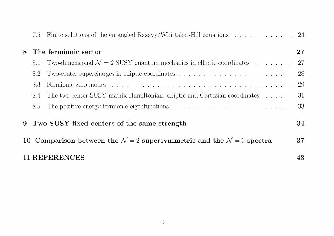
1 The classical (Euler) problem of two Newtonian/Coulombian fixed centers

Figure 1: Location of the two centers and distances to the particle from the centers.

• The classical action:

S =

∫dt

{1

2m

(dx1

dt

dx1

dt+dx2

dt

dx2

dt

)+α1

r1+α2

r2

}

center locations (x1 = −d, x2 = 0) , (x1 = d, x2 = 0)

center strengths α1 = α ≥ α2 = δα > 0 , δ ∈ (0, 1]

distances to centers r1 =√

(x1 − d)2 + x22 , r2 =

√(x1 + d)2 + x2

2

4

• Dimensions of the coupling constants and parameters and non-dimensional variables:

[α1] = [α2] = [α] = ML3T−2 , [d] = L , [δ] = 1

x1 → d x1 , x2 → d x2 , t→√d3m

αt ,

r1 → d r1 = d√

(x1 − 1)2 + x22 , r2 → d r2 = d

√(x1 + 1)2 + x2

2

• Non-dimensional action:

S =√mdαS =

√mdα

∫dt

{1

2

(dx1

dt

dx1

dt+dx2

dt

dx2

dt

)+

1

r1+δ

r2

}

• Linear momenta and Hamiltonian: p1 = ∂L∂x1

= dx1dt , p2 = ∂L

∂x2= dx2

dt

H =α

dH , H =

1

2(p2

1 + p22)− 1

r1− δ

r2

• The second invariant:

I2 = (mdα)I2 , I2 =1

2(l2−p2

2)+x1

(δ

r2− 1

r1

)+

(1

r1+δ

r2

), l2 = (x1p2−x2p1)2

5

2 The quantum problem (N = 0) of two Coulombian centers

• Canonical quantization

pi → pi = −i~ ∂

∂xi, xi → xi = xi

[xi, pj] = i~δij , ~ =~√mdα

.

• Quantum Hamiltonian, ˆH = αdH , and quantum symmetry operator, ˆI2 = (mdα)I2, are the mutua-

lly commuting operators:

H = −~2

(∂2

∂x21

+∂2

∂x22

)− 1

r1− δ

r2, [H, I2] = HI2 − I2H = 0

I2 = −~2

2

((x2

1 − 1)∂2

∂x22

+ x22

∂2

∂x21

− 2x1x2∂2

∂x1∂x2− x1

∂

∂x1− x2

∂

∂x2

)+x1

(δ

r2− 1

r1

)+

(1

r1+δ

r2

)

6

3 The N = 0 spectral problem in elliptic coordinates: Razavy and Whittaker-Hill

equations

• Elliptic coordinates

x1 = uv ∈ (−∞,+∞) , x2 = ±√

(u2 − 1)(1− v2) ∈ (−∞,+∞)

u =1

2(r1 + r2) ∈ (1,+∞) , v =

1

2(r2 − r1) ∈ (−1, 1)

• The Hamiltonian in elliptic coordinates

H =−~2

2(u2 − v2)

((u2 − 1)

∂2

∂u2+ u

∂

∂u+ (1− v2)

∂2

∂v2− v ∂

∂v

)− ((1 + δ)u + (1− δ)v)

(u2 − v2)

7

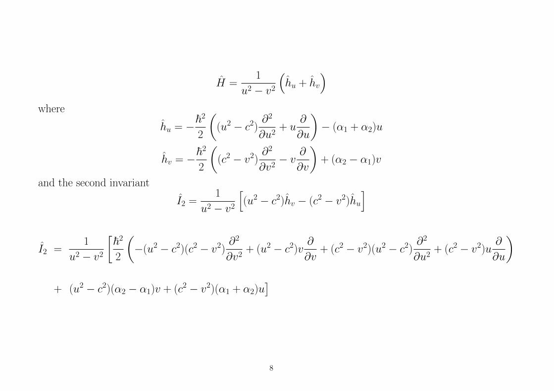
H =1

u2 − v2

(hu + hv

)where

hu = −~2

2

((u2 − c2)

∂2

∂u2+ u

∂

∂u

)− (α1 + α2)u

hv = −~2

2

((c2 − v2)

∂2

∂v2− v ∂

∂v

)+ (α2 − α1)v

and the second invariant

I2 =1

u2 − v2

[(u2 − c2)hv − (c2 − v2)hu

]

I2 =1

u2 − v2

[~2

2

(−(u2 − c2)(c2 − v2)

∂2

∂v2+ (u2 − c2)v

∂

∂v+ (c2 − v2)(u2 − c2)

∂2

∂u2+ (c2 − v2)u

∂

∂u

)

+ (u2 − c2)(α2 − α1)v + (c2 − v2)(α1 + α2)u]

8

• Spectral problem and separation ansatz:

HψE(u, v) = EψE(u, v) , ψE(u, v) = η(u)ξ(v)

−~2(u2 − 1)η′′(u)− ~2uη′(u)−[2(1 + δ)u + 2u2E

]η(u) = Iη(u)

−~2(1− v2)ξ′′(v) + ~2vξ′(v) +[−2(1− δ)v + 2v2E

]ξ(v) = −Iξ(v)

I eigenvalue of the symmetry operator I = −H − I2.

9

• Razavy equation

−d2η(x)

dx2+ (ζ cosh 2x−M)2 η(x) = λη(x) , x =

1arccoshu ∈ [0,∞)

ζ =2√

2|E|~

, λ = M 2 +4I

~2, M 2 =

2(1 + δ)2

~2|E|

F. Finkel, A. Gonzalez-Lopez and M. A. Rodrıguez, Journal of Physics A: Math. Gen. 32(1999)6821-6835.

M. Razavy, Am. J. Phys. 48(1980)285; Phys. Lett. 82A(1981)7.

• Whittaker-Hill equation

d2ξ(y)

dy2+ (β cos2y −N)2ξ(y) = µξ(y) , y =

1

2arccosv ∈ [0,

π

2]

β = −2√

2|E|~

, µ = N 2 +4I

~2, N 2 =

2(1− δ)2

~2|E|

10

4 Finite solutions of the Razavy equation

• If M = n+1, n ∈ N, the Razavy equation is a quasi exactly solvable (QES) system: n+1 solutions

for n + 1 values of λ are known.

• Solution of the Razavy equation by series expansion

ηn(z) = z1−(n+1)

2 e−ζ4(z+1

z)∞∑k=0

(−1)k Pk(λ)

(2ζ)k k!zk , z = e2x

• Recurrence relations:

Pk+1(λ) =(λ− (4k(n− k) + 2n + 1 + ζ2)

)Pk(λ)− (4k(n + 1− k)ζ2)Pk−1(λ) , k ≥ 0

• Finite solutions

If λnm is a root of Pn+1, Pn+1(λnm) = 0, m = 1, 2, · · ·n + 1,

0 = Pn+2(λnm) = Pn+3(λnm) = . . .

and the series truncates.

11

• Lower cases:

• n = 0:

ζ0 = 4~2(1 + δ) , λ01 = 1 + ζ2

0 , η01(x) = e−ζ02 cosh 2x

• n = 1:

ζ1 = 2~2(1 + δ) , λ11 = 3− 2ζ1 + ζ2

1 , λ12 = 3 + 2ζ1 + ζ21

η11(x) = 2e−ζ12 cosh 2x coshx , η12(x) = −2e−

ζ12 cosh 2x sinhx

• n = 2

ζ2 =4

3~2(1 + δ) , λ21 = ζ2

2 + 5 , λ22 = ζ22 + 7− 2

√1 + 4ζ2

2 , λ23 = ζ22 + 7 + 2

√1 + 4ζ2

2

η21(x) = −2e−ζ22 cosh 2x sinh 2x

η22(x) = 1ζ2e−

ζ22 cosh 2x

(2ζ2 cosh 2x− 1 +

√1 + 4ζ2

2

)η23(x) = 1

ζ2e−

ζ22 cosh 2x

(2ζ2 cosh 2x− 1−

√1 + 4ζ2

2

)12

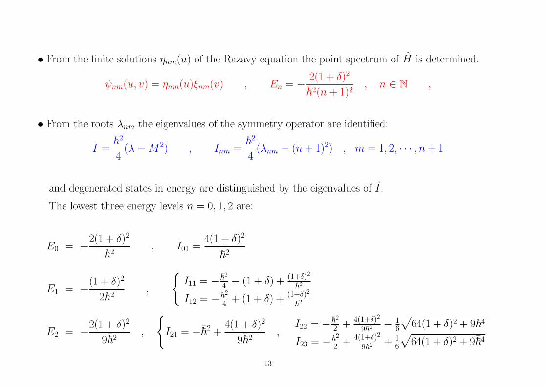
• From the finite solutions ηnm(u) of the Razavy equation the point spectrum of H is determined.

ψnm(u, v) = ηnm(u)ξnm(v) , En = − 2(1 + δ)2

~2(n + 1)2, n ∈ N ,

• From the roots λnm the eigenvalues of the symmetry operator are identified:

I =~2

4(λ−M 2) , Inm =

~2

4(λnm − (n + 1)2) , m = 1, 2, · · · , n + 1

and degenerated states in energy are distinguished by the eigenvalues of I .

The lowest three energy levels n = 0, 1, 2 are:

E0 = −2(1 + δ)2

~2, I01 =

4(1 + δ)2

~2

E1 = −(1 + δ)2

2~2,

{I11 = − ~2

4 − (1 + δ) + (1+δ)2

~2

I12 = − ~2

4 + (1 + δ) + (1+δ)2

~2

E2 = −2(1 + δ)2

9~2,

{I21 = −~2 +

4(1 + δ)2

9~2,

I22 = − ~2

2 + 4(1+δ)2

9~2 − 16

√64(1 + δ)2 + 9~4

I23 = − ~2

2 + 4(1+δ)2

9~2 + 16

√64(1 + δ)2 + 9~4

13

The ξnm(v) solutions of the Razavy trigonometric or Whittaker-Hill equation for E = En and I = Inm

are given as infinite series.

Ground state

β0 = − 4

~2(1 + δ) , N 2

0 =

(1− δ1 + δ

)

5 Two centers of the same strength: the Mathieu equation

The case of two centers of equal force δ → 1 is easier, v = 12(r2 − r1) becomes cyclic.

• The Whittaker-Hill equation becomes the Mathieu equation:

−d2ξ(y)

dy2+ (α cos4y + σ)ξ(y) = 0

α =4E

~2, σ =

4

~2(I + E)

14

• The characteristic values (a, q) of Mathieu functions, C[a, q, y] and S[a, q, y], are fixed by the values

of En and Inm, obtained from the finite solutions ηnm(u) of the Razavy equation:

anm = −En + Inm~2

= −σnm4

, qn =En

2~2=αn8

.

• even/odd (in v) solutions of the Mathieu equations:

ξnm ,even(v) =c1

2(C [anm, qn, arccos(v)] + C [anm, qn, arccos(−v)])

+c2

2(S [anm, qn, arccos(v)] + S [anm, qn, arccos(−v)])

ξnm ,odd(v) =d1

2(C [anm, qn, arccos(v)]− C [anm, qn, arccos(−v)])

+d2

2(S [anm, qn, arccos(v)]− S [anm, qn, arccos(−v)])

Reason: invariance of the problem under r1 ↔ r2 ≡ v ↔ −v.

• E0 = − 8~2

15

I01 =16

~2; ψ01(u, v) = e

−4u~2 ξ01 ,even/odd(v) , q0 = − 4

~4, a01 = − 8

~4

• E1 = − 2~2{

I11 = − ~2

4 − 2 + 4~2

I12 = − ~2

4 + 2 + 4~2

;

{ψ11(u, v) = e

−2u~2√

2(u + 1) ξ11 ,even/odd(v)

ψ12(u, v) = −e−2u~2√

2(u− 1) ξ12 ,even/odd(v)

q1 = − 1~4 ,

{a11 = − 2

~4 + 2~2 + 1

4

a12 = − 2~4 − 2

~2 + 14

• E2 = − 89~2

{I21 = −~2 + 16

9~2 ,I22 = − ~2

2 + 169~2 − 1

6

√256 + 9~4

I23 = − ~2

2 + 169~2 + 1

6

√256 + 9~4

η21(u) = −2e− 4u

3~2√u2 − 1 ,

η22(u) = 3~2

8 e− 4u

3~2

[163~2u− 1 +

√1 + 256

9~4

]η23(u) = 3~2

8 e− 4u

3~2

[163~2u− 1−

√1 + 256

9~4

]16

q2 = − 49~4 ,

{a21 = 1− 8

9~4 ,a22 = 1

2 −8

9~4 + 16~2

√256 + 9~4

a23 = 12 −

89~4 − 1

6~2

√256 + 9~4

17

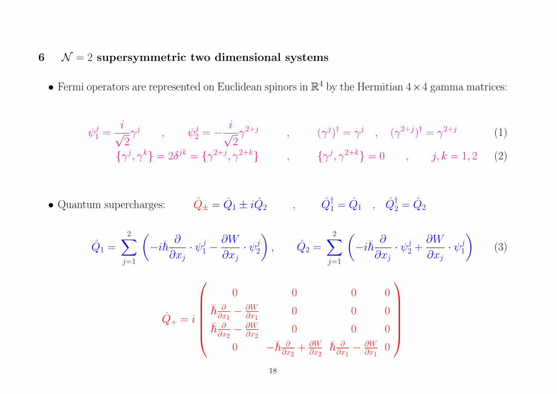
6 N = 2 supersymmetric two dimensional systems

• Fermi operators are represented on Euclidean spinors in R4 by the Hermitian 4×4 gamma matrices:

ψj1 =i√2γj , ψj2 = − i√

2γ2+j , (γj)† = γj , (γ2+j)† = γ2+j (1)

{γj, γk} = 2δjk = {γ2+j, γ2+k} , {γj, γ2+k} = 0 , j, k = 1, 2 (2)

• Quantum supercharges: Q± = Q1 ± iQ2 , Q†1 = Q1 , Q†2 = Q2

Q1 =

2∑j=1

(−i~ ∂

∂xj· ψj1 −

∂W

∂xj· ψj2), Q2 =

2∑j=1

(−i~ ∂

∂xj· ψj2 +

∂W

∂xj· ψj1)

(3)

Q+ = i

0 0 0 0

~ ∂∂x1− ∂W

∂x10 0 0

~ ∂∂x2− ∂W

∂x20 0 0

0 −~ ∂∂x2

+ ∂W∂x2

~ ∂∂x1− ∂W

∂x10

18

Q− = i

0 ~ ∂

∂x1+ ∂W

∂x1~ ∂∂x2

+ ∂W∂x2

0

0 0 0 −~ ∂∂x2− ∂W

∂x2

0 0 0 ~ ∂∂x1

+ ∂W∂x1

0 0 0 0

• SUSY algebra

{Q+, Q−} = 2HS , [Q+, HS] = [Q−, HS] = 0 (4)

• Quantum SUSY Hamiltonian and Fermi number F =

2∑j=1

ψj+ψj− operators:

HS =

h(0) 0 0 0

0 h(1)11 h

(1)12 0

0 h(1)21 h

(1)22 0

0 0 0 h(2)

, F =

2∑j=1

ψj+ψj− =

0 0 0 0

0 1 0 0

0 0 1 0

0 0 0 2

(5)

19

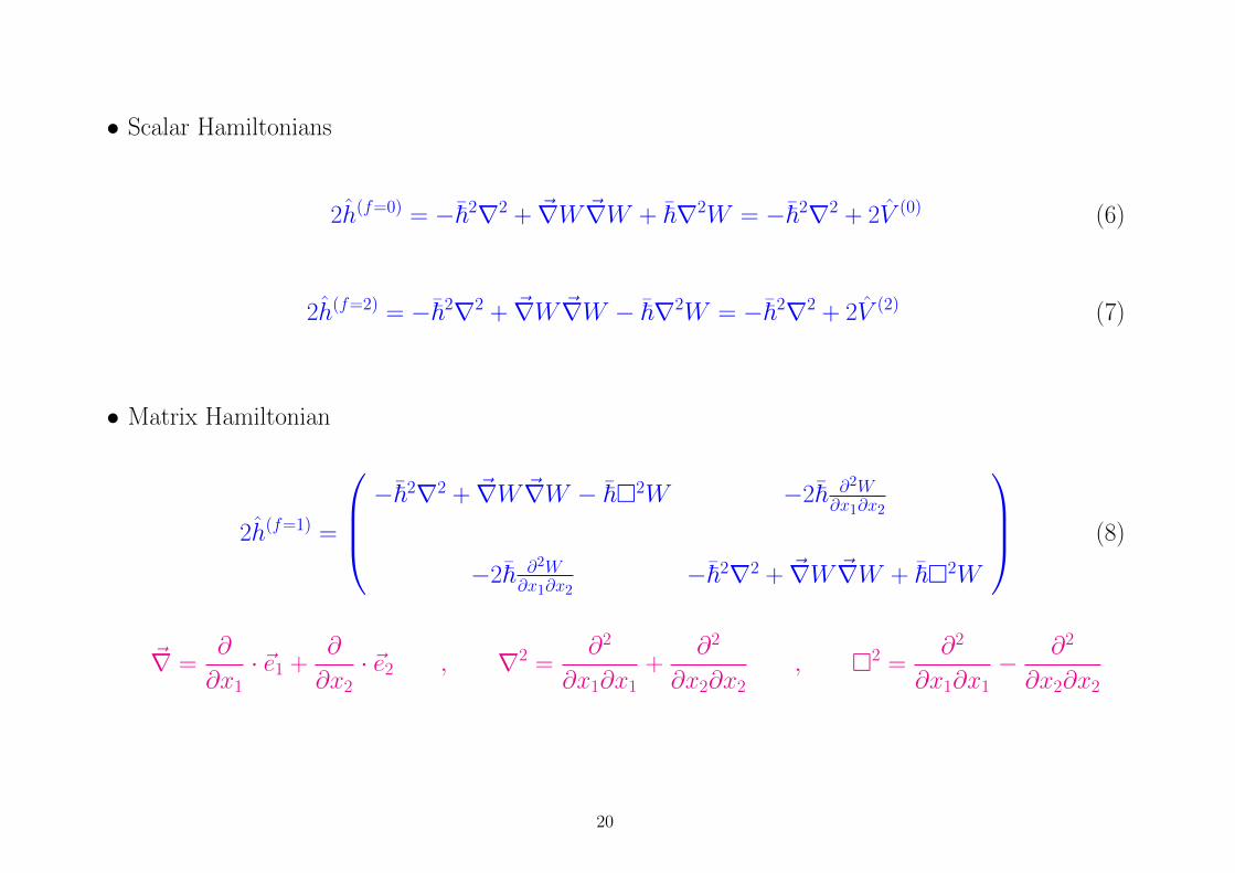
• Scalar Hamiltonians

2h(f=0) = −~2∇2 + ~∇W ~∇W + ~∇2W = −~2∇2 + 2V (0) (6)

2h(f=2) = −~2∇2 + ~∇W ~∇W − ~∇2W = −~2∇2 + 2V (2) (7)

• Matrix Hamiltonian

2h(f=1) =

−~2∇2 + ~∇W ~∇W − ~�2W −2~ ∂2W

∂x1∂x2

−2~ ∂2W∂x1∂x2

−~2∇2 + ~∇W ~∇W + ~�2W

(8)

~∇ =∂

∂x1· ~e1 +

∂

∂x2· ~e2 , ∇2 =

∂2

∂x1∂x1+

∂2

∂x2∂x2, �2 =

∂2

∂x1∂x1− ∂2

∂x2∂x2

20

7 N = 2 supersymmetric two 2D fixed centers of force

7.1 The superpotential for the two center problem

• Poisson equation:~2∇2W = − 1

r1− δ

r2. (9)

• “Elliptic” and “Cartesian” superpotential

W (u, v) = −2(1 + δ)u

~+

2(1− δ)v

~, W (x1, x2) = −2r1

~− 2δr2

~, (10)

7.2 Bosonic zero modes

Q±Ψ(0)0 (x1, x2) = 0 , Q∓Ψ

(2)0 (x1, x2) = 0

21

Ψ(0)0 (x1, x2) = exp[−2

~(r1 + δr2)]

1

0

0

0

, Ψ(2)0 (x1, x2) = exp[

2

~(r1 + δr2)]

0

0

0

1

• Finite norm

N 2(~) = 2

∫ ∞1

du

∫ 1

−1

dv

(e− 4

~2 (1+δ)u√u2 − 1

e4~2 (1−δ)v√

1− v2+e− 4

~2 (1+δ)u

√u2 − 1

e4~2 (1−δ)v√

1− v2

)

N 2(~) = 2π

[~2

4(1 + δ)I0

(4

~2(1− δ)

)K1

(4

~2(1 + δ)

)+

~2

4(1− δ)I1

(4

~2(1− δ)

)K0

(4

~2(1 + δ)

)].

7.3 The two-center SUSY scalar Hamiltonians: elliptic and Cartesian coordinates

• Scalar Hamiltonians:

h((0)(2)) =

1

2(u2 − v2)

{−~2

((u2 − 1)

∂2

∂u2+ u

∂

∂u+ (1− v2)

∂2

∂v2− v ∂

∂v

)(11)

+

(4

~2((1 + δ)2(u2 − 1) + (1− δ)2(1− v2))∓ 2((1 + δ)u + (1− δ)v)

)}22

h((0)(2)) = −~

2

2∇2 +

2

~2

[1 + δ2 + δ

(r1

r2+r2

r1− 4

r1r2

)]∓(

1

r1+δ

r2

),

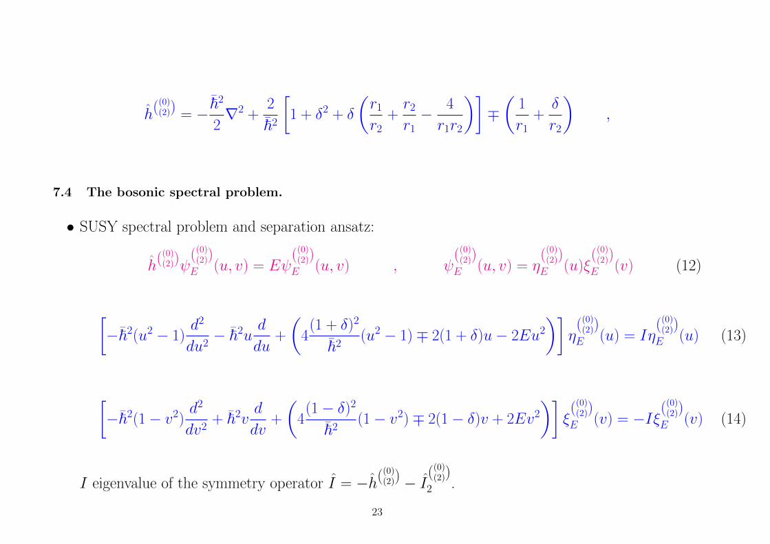
7.4 The bosonic spectral problem.

• SUSY spectral problem and separation ansatz:

h((0)(2))ψ

((0)(2))E (u, v) = Eψ

((0)(2))E (u, v) , ψ

((0)(2))E (u, v) = η

((0)(2))E (u)ξ

((0)(2))E (v) (12)

[−~2(u2 − 1)

d2

du2− ~2u

d

du+

(4

(1 + δ)2

~2(u2 − 1)∓ 2(1 + δ)u− 2Eu2

)]η

((0)(2))E (u) = Iη

((0)(2))E (u) (13)

[−~2(1− v2)

d2

dv2+ ~2v

d

dv+

(4

(1− δ)2

~2(1− v2)∓ 2(1− δ)v + 2Ev2

)]ξ((0)

(2))E (v) = −Iξ

((0)(2))E (v) (14)

I eigenvalue of the symmetry operator I = −h((0)(2)) − I

((0)(2))

2 .

23

• Razavy equations

−d2η±(x)

dx2+ (ζ± cosh 2x−M±)2 η±(x) = λ± η±(x) , x =

1

2arccoshu ∈ [0,∞) (15)

ζ± = ±2

~

√4

~2(1 + δ)2 − 2E± , λ± = M 2

± +4

~2(I± + 4

(1 + δ)2

~2) , M 2

± =2(1 + δ)2

2(1 + δ)2 − ~2E±

• Whittaker-Hill equation

d2ξ±(y)

dy2+ (β±cos2y −N±)2 ξ±(y) = µ± ξ±(y) , y =

1

2arccosv ∈ [0,

π

2] (16)

β± = ∓2

~

√4

~2(1− δ)2 − 2E± , N 2

± =2(1− δ)2

2(1− δ)2 − ~2E±, µ± = N 2

±+4

~2(I±+

4

~2(1− δ)2)

7.5 Finite solutions of the entangled Razavy/Whittaker-Hill equations

• M± = n± + 1, n± ∈ N : QES systems

E± = 2(1 + δ)2

~2

(1− 1

(n± + 1)2

),

24

• Lower eigenvalues and eigen-functions of h(0) and h(2): E0 = 0, E1 = 32~2(1 + δ)2, E2 = 16

9~2(1 +

δ)2, · · ·, n± = 0, 1, 2, · · ·:

η01± (u) = e

∓2(1+δ)u

~2 ,

η11± (u) = e

∓ (1+δ)u

~2√

2(u + 1)

η12± (u) = −e∓

(1+δ)u

~2√

2(u− 1)η21± (u) = −2e

∓2(1+δ)u

3~2√u2 − 1 ,

η22± (u) = ± 3~2

4(1+δ)e∓2(1+δ)u

3~2

[±8(1+δ)

3~2 u− 1 +√

1 + 64(1+δ)2

9~4

]

η23± (u) = ± 3~2

4(1+δ)e∓2(1+δ)u

3~2

[±8(1+δ)

3~2 u− 1−√

1 + 64(1+δ)2

9~4

]• The degeneracy in the energy is broken by the eigenvalues of the second invariant I±,

I± =~2

4(λ± −M±)2 − 4

~2(1 + δ)2

In±m± =~2

4(λn±m± − (n± + 1)2)− 4

~2(1 + δ)2 , m± = 1, 2, · · · , n± + 1 ,

25

labeling different eigenfunctions of the same energy:

I01± = 0 ,

I11± = − ~2

4 −3(1+δ)2

~2 ∓ (1 + δ)

I12± = − ~2

4 −3(1+δ)2

~2 ± (1 + δ)I21± = −~2 − 32(1 + δ)2

9~2,

I22± = − ~2

2 −32(1+δ)2

9~2 − 16

√64(1 + δ)2 + 9~4

I23± = − ~2

2 −32(1+δ)2

9~2 + 16

√64(1 + δ)2 + 9~4

• Bosonic zero modes

If n+ = 0,

E+(n+ = 0) = 2(1 + δ)2

~2

(1− 1

(n+ + 1)2

)= 0

the Whittaker-Hill equation is also QES with a unique finite wave function:

β+0 = − 4

~2(1− δ) , N+0 = 1 , ξ01

+ (v) = e2(1−δ)~2 v

Also, In+=0,m+=1 = 0. Thus,

E0 = 0 , ψ01+ (u, v) = exp[−2(1 + δ)u

~2] · exp[±2(1− δ)v

~2]

26

and ψ01+ (u, v) is the normalizable zero energy ground state of two SUSY centers.

SUPERSYMMETRY IS UNBROKEN

• If n+ > 0, the Whittaker-Hill equation is not QES and only infinite series give the ξ(v) factor of

the eigen-functions.

• There is no point spectrum in h(2).

8 The fermionic sector

8.1 Two-dimensional N = 2 SUSY quantum mechanics in elliptic coordinates

• Induced metric by the map R2 ≡ (−∞,+∞)× (−∞,+∞) =⇒ E2 ≡ (−1, 1)× (1,+∞):

g(u, v) =

guu =u2 − v2

u2 − 1guv = 0

gvu = 0 gvv =u2 − v2

1− v2

, g−1(u, v) =

guu =u2 − 1

u2 − v2guv = 0

gvu = 0 gvv =1− v2

u2 − v2

(17)

Γuuu =−u(1− v2)

(u2 − v2)(u2 − 1), Γvvv =

v(u2 − 1)

(u2 − v2)(1− v2), Γuuv = Γuvu =

−vu2 − v2

Γvuu =v(1− v2)

(u2 − v2)(u2 − 1), Γuvv =

−u(u2 − 1)

(u2 − v2)(1− v2), Γvuv = Γvvu =

u

u2 − v2

.

27

• ” Spinors and “elliptic” Fermi operators:

Zweig-bein:

guu(u, v) =

2∑j=1

euj (u, v)euj (u, v) , gvv(u, v) =

2∑j=1

evj(u, v)evj(u, v)

eu1(u, v) =

(u2 − 1

u2 − v2

)12

, ev2(u, v) =

(1− v2

u2 − v2

)12

ψu±(u, v) = eu1(u, v)ψ1± , ψv±(u, v) = ev2(u, v)ψ2

± . (18)

8.2 Two-center supercharges in elliptic coordinates

C+ = −i√~

0 0 0 0

eu1∇−u 0 0 0

ev2∇−v 0 0 0

0 −ev2(∇−v − ~v

u2−v2

)eu1

(∇−u + ~u

u2−v2

)0

, ∇∓u = ~∂

∂u∓ dF

du, F (u) = −2(1 + δ)

~2u

28

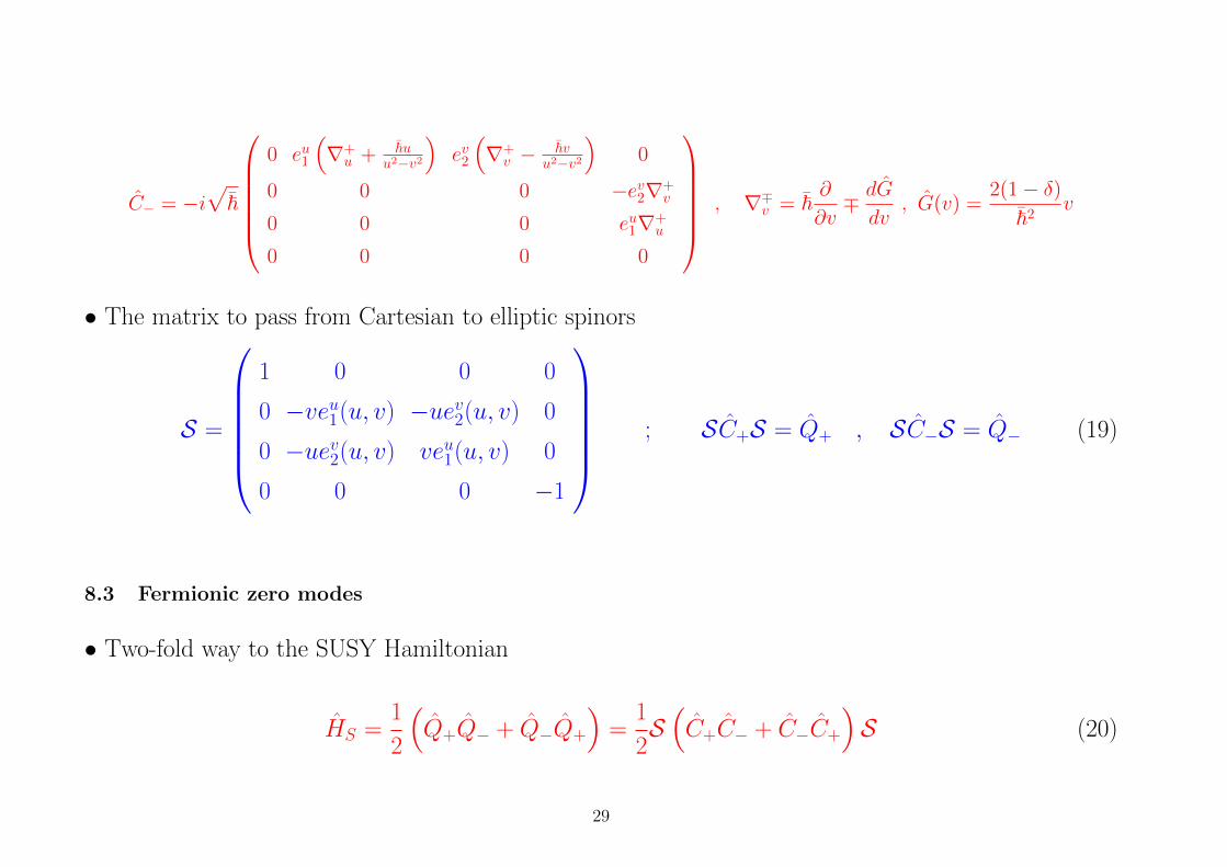
C− = −i√~

0 eu1

(∇+u + ~u

u2−v2

)ev2

(∇+v − ~v

u2−v2

)0

0 0 0 −ev2∇+v

0 0 0 eu1∇+u

0 0 0 0

, ∇∓v = ~∂

∂v∓ dG

dv, G(v) =

2(1− δ)~2

v

• The matrix to pass from Cartesian to elliptic spinors

S =

1 0 0 0

0 −veu1(u, v) −uev2(u, v) 0

0 −uev2(u, v) veu1(u, v) 0

0 0 0 −1

; SC+S = Q+ , SC−S = Q− (19)

8.3 Fermionic zero modes

• Two-fold way to the SUSY Hamiltonian

HS =1

2

(Q+Q− + Q−Q+

)=

1

2S(C+C− + C−C+

)S (20)

29

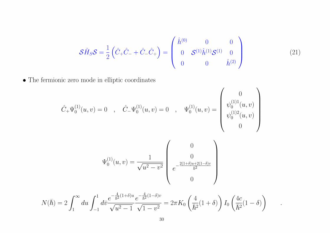
SHSS =1

2

(C+C− + C−C+

)=

h(0) 0 0

0 S(1)h(1)S(1) 0

0 0 h(2)

(21)

• The fermionic zero mode in elliptic coordinates

C+Ψ(1)0 (u, v) = 0 , C−Ψ

(1)0 (u, v) = 0 , Ψ

(1)0 (u, v) =

0

ψ(1)10 (u, v)

ψ(1)20 (u, v)

0

Ψ(1)0 (u, v) =

1√u2 − v2

0

0

e−2(1+δ)u+2(1−δ)v

~2

0

N(~) = 2

∫ ∞1

du

∫ 1

−1

dve− 4

~2 (1+δ)u

√u2 − 1

e− 4

~2 (1−δ)v√

1− v2= 2πK0

(4

~2(1 + δ)

)I0

(4c

~2(1− δ)

).

30

• The Fermionic zero mode in Cartesian coordinates

Ψ(1)0 (x1, x2) = SΨ

(1)0 (r1, r2) =

0

−(r1+r2)4√r1r2

√4

r1r2− r1

r2− r2

r1+ 2

(r2−r1)4√r1r2

√− 4r1r2

+ r1r2

+ r2r1

+ 2

0

· e−2(δr1+r2)

~2 .

8.4 The two-center SUSY matrix Hamiltonian: elliptic and Cartesian coordinates

• Matrix Hamiltonian:

(S(1)h(1)S(1))11 = − ~2

2(u2 − v2)

(−(u2 − 1)

∂2

∂u2− u ∂

∂u− (1− v2)

∂2

∂v2+ v

∂

∂v

)+ ~2 u

2 + v2 − 1

2(u2 − v2)2

+

(2((1 + δ)2(u2 − 1) + (1− δ)2(1− v2))

~2(u2 − v2)− ((1 + δ)u + (1− δ)v)(u2 + v2 − 2)

(u2 − v2)2

)

(S(1)h(1)S(1))12 =~2√

(u2 − 1)(1− v2)

(u2 − v2)2

(u∂

∂v+ v

∂

∂u

)+ 2

((1− δ)u + (1 + δ)v)√

(u2 − 1)(1− v2)

(u2 − v2)2

(S(1)h(1)S(1))21 = −~2√

(u2 − 1)(1− v2)

(u2 − v2)2

(u∂

∂v+ v

∂

∂u

)+ 2

((1− δ)u + (1 + δ)v)√

(u2 − 1)(1− v2)

(u2 − v2)2

31

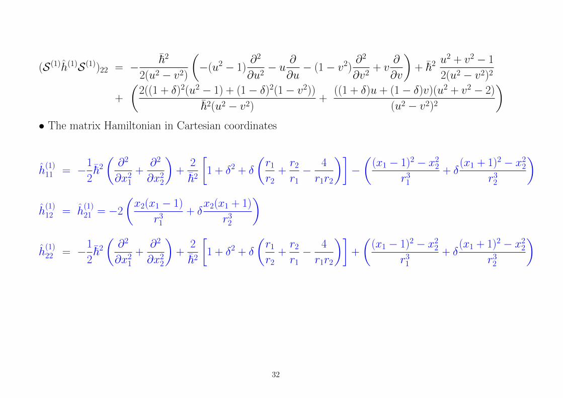
(S(1)h(1)S(1))22 = − ~2

2(u2 − v2)

(−(u2 − 1)

∂2

∂u2− u ∂

∂u− (1− v2)

∂2

∂v2+ v

∂

∂v

)+ ~2 u

2 + v2 − 1

2(u2 − v2)2

+

(2((1 + δ)2(u2 − 1) + (1− δ)2(1− v2))

~2(u2 − v2)+

((1 + δ)u + (1− δ)v)(u2 + v2 − 2)

(u2 − v2)2

)• The matrix Hamiltonian in Cartesian coordinates

h(1)11 = −1

2~2

(∂2

∂x21

+∂2

∂x22

)+

2

~2

[1 + δ2 + δ

(r1

r2+r2

r1− 4

r1r2

)]−(

(x1 − 1)2 − x22

r31

+ δ(x1 + 1)2 − x2

2

r32

)

h(1)12 = h

(1)21 = −2

(x2(x1 − 1)

r31

+ δx2(x1 + 1)

r32

)

h(1)22 = −1

2~2

(∂2

∂x21

+∂2

∂x22

)+

2

~2

[1 + δ2 + δ

(r1

r2+r2

r1− 4

r1r2

)]+

((x1 − 1)2 − x2

2

r31

+ δ(x1 + 1)2 − x2

2

r32

)

32

8.5 The positive energy fermionic eigenfunctions

• Fermionic spectral problem

S(1)h(1)S(1)

(ψ

(1)1E (u, v)

ψ(1)2E (u, v)

)= E

(ψ

(1)1E (u, v)

ψ(1)2E (u, v)

)• Fermionic bound states in elliptic coordinates

Ψ(1)En+

(u, v) = C+Ψ(0)En+

(u, v) =

0

ψ(1)1En+

(u, v)

ψ(1)2En+

(u, v)

0

= −i

0

eu1∇−uψ(0)En+

(u, v)

ev2∇−v ψ(0)En+

(u, v)

0

• Fermionic bound states in Cartesian coordinates

Ψ(1)En+

(x1, x2) = Q+Ψ(0)En+

(x1, x2) =

0

ψ(1)1En+

(x1, x2)

ψ(1)2En+

(x1, x2)

0

= −i

0

(~ ∂∂x1− ∂W

∂x1)ψ

(0)En+

(x1, x2)

(~ ∂∂x2− ∂W

∂x2)ψ

(0)En+

(x1, x2)

0

Ψ

(1)En+

(x1, x2) = SΨ(1)En+

(u, v)

33

9 Two SUSY fixed centers of the same strength

• The SUSY spectral problem[−~2(u2 − 1)

d2

du2− ~2u

d

du+

(16

~2(u2 − 1)∓ 4u− 2Eu2

)]η

((0)(2))E (u) = Iη

((0)(2))E (u) (22)[

−~2(1− v2)d2

dv2+ ~2v

d

dv+ 2Ev2

]ξ((0)

(2))E (v) = −Iξ

((0)(2))E (v) (23)

• The Razavy and Mathieu equations

−d2η±(x)

dx2+ (ζ± cosh 2x−M±)2 η±(x) = λ± η±(x) , (24)

ζ± = ±2

~

√16

~2− 2E± , M 2

± =8

8− ~2E±, λ± = M 2

± +4

~2(I± +

16

~2) ,

−d2ξ±(y)

dy2+ (α± cos4y + σ±) ξ±(y) = 0 (25)

α± =4E±~2

, σ± =4

~2(I± + E) ,

34

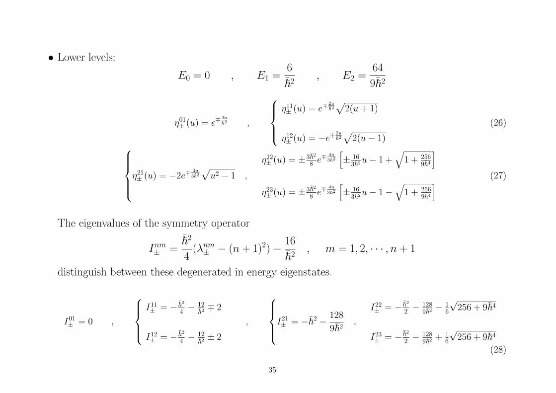
• Lower levels:

E0 = 0 , E1 =6

~2, E2 =

64

9~2

η01± (u) = e∓

4u~2 ,

η11± (u) = e∓

2u~2

√2(u+ 1)

η12± (u) = −e∓

2u~2

√2(u− 1)

(26)

η21± (u) = −2e∓

4u3~2

√u2 − 1 ,

η22± (u) = ±3~2

8 e∓ 4u

3~2

[± 16

3~2u− 1 +√

1 + 2569~4

]η23± (u) = ±3~2

8 e∓ 4u

3~2

[± 16

3~2u− 1−√

1 + 2569~4

] (27)

The eigenvalues of the symmetry operator

Inm± =~2

4(λnm± − (n + 1)2)− 16

~2, m = 1, 2, · · · , n + 1

distinguish between these degenerated in energy eigenstates.

I01± = 0 ,

I11± = − ~2

4 −12~2 ∓ 2

I12± = − ~2

4 −12~2 ± 2

,

I21± = −~2 − 128

9~2,

I22± = − ~2

2 −1289~2 − 1

6

√256 + 9~4

I23± = − ~2

2 −1289~2 + 1

6

√256 + 9~4

(28)

35

• Even/odd in v solutions of the Mathieu equations

ξnm±even(v) =c1

2(C [anm± , qn, arccos(v)] + C [anm± , qn, arccos(−v)])

+c2

2(S [anm± , qn, arccos(v)] + S [anm± , qn, arccos(−v)]) (29)

ξnm±odd(v) =d1

2(C [anm± , qn, arccos(v)]− C [anm± , qn, arccos(−v)])

+d2

2(S [anm± , qn, arccos(v)]− S [anm± , qn, arccos(−v)]) (30)

The parameters of the Mathieu equations determined by the spectral problem are:

anm± = −σnm±

4= −

En + Inm±~2

, qn =αn8

=En

2~2

q0 = 0 , a01± = 0

q1 = 3~4 ,

{a11± = 6

~4 ± 2~2 + 1

4

a12± = 6

~4 ∓ 2~2 + 1

4

q2 = 329~4 ,

{a21± = 1 + 64

9~4 ,a22± = 1

2 + 649~4 + 1

6~2

√256 + 9~4

a23± = 1

2 + 649~4 − 1

6~2

√256 + 9~4

36

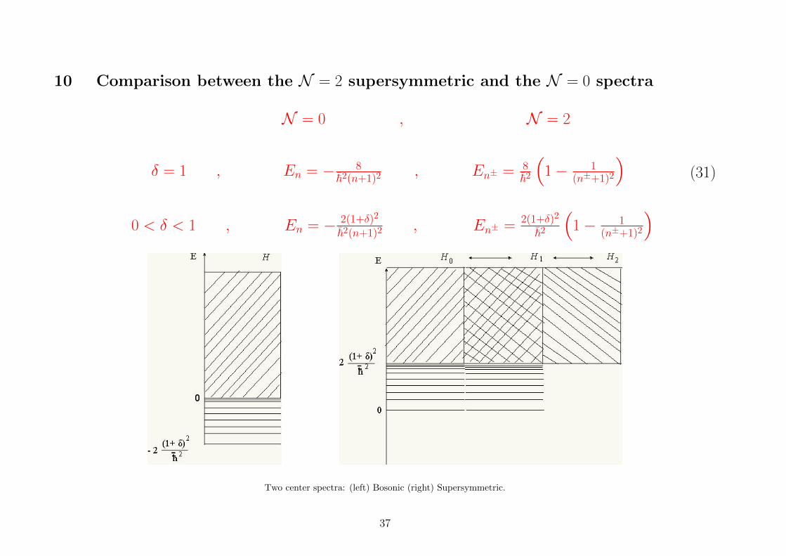
10 Comparison between the N = 2 supersymmetric and the N = 0 spectra

N = 0 , N = 2

δ = 1 , En = − 8~2(n+1)2 , En± = 8

~2

(1− 1

(n±+1)2

)0 < δ < 1 , En = − 2(1+δ)2

~2(n+1)2 , En± = 2(1+δ)2

~2

(1− 1

(n±+1)2

)(31)

Two center spectra: (left) Bosonic (right) Supersymmetric.

37

Table 1: N = 0 and δ = 1|ψnm(x1, x2)|2 ~ = 0.7 ~ = 1 ~ = 2 ~ = 4

n=0, m=1 (even)

n=0, m=1 (odd)

Table 2: Supersymmetric N = 2 and δ = 1

|ψnm+ (x1, x2)|2 ~ = 0.7 ~ = 1 ~ = 2 ~ = 4

n=0, m=1 (only even)

38

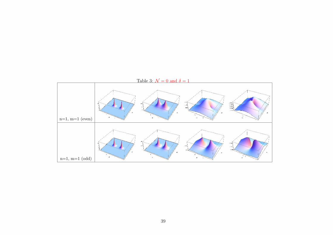
Table 3: N = 0 and δ = 1

n=1, m=1 (even)

n=1, m=1 (odd)

39

Table 4: Supersymmetric N = 2 and δ = 1

n=1, m=1 (even)

n=1, m=1 (odd)

40

Table 5: N = 0 and δ = 1

n=2, m=1 (even)

n=2, m=1 (odd)

41

Table 6: Supersymmetric N = 2 and δ = 1

n=2, m=1 (even)

n=2, m=1 (odd)

42

11 REFERENCES

1. A. Perelomov, Integrable Systems of Classical Mechanics and Lie Algebras, Birkhauser, (1992).

2. F. Finkel, A. Gonzalez-Lopez and M. A. Rodrıguez, Journal of Physics A: Math. Gen. 32(1999)6821-6835.

3. M. Razavy, Am. J. Phys. 48(1980)285.

4. M. Razavy, Phys. Lett. 82A(1981)7.

5. A. Andrianov, N. Borisov, and M. Ioffe, Physics Letters A105(1984)19, Theoretical and Mathematical Physics 61(1984) 963

6. A. Andrianov, N. Borisov, M. Eides and M. Ioffe, Physics Letters A109(1985)143, Theoretical and Mathematical Physics 61(1984)1078

7. A. Kirchberg, J. Lange, P. Pisani, and A. Wipf, Annals of Physics 303(82003)359

8. A. Wipf, A. Kirchberg and J.D. Lange, Proceedings of the 4th International Symposium ”Quantum Theory and Symmetries” (QTS-4),

15-21 August 2005, Varna, Bulgaria. hep-th/0511231.

9. A. Alonso Izquierdo, M. A. Gonzalez Leon, J. Mateos Guilarte, and M. de la Torre Mayado, Annals of Physics 308(2003)664, Journal

of Physics A37(2004)10323

10. D. Bondar, M.Hnatic, and V. Lazur, Theoretical and Mathematical Physics 148(2006)1011

11. M. A. Gonzalez Leon, J. Mateos Guilarte, and M. de la Torre Mayado, SIGMA 3(2007)124, 24 pages

43