Math 5470 § 1.Treibergs

First Midterm Exam Name: Practice ProblemsJanuary 11, 2016

1. Analyze the equation graphically. Find all fixed points, classify their stability and sketch thegraph for different initial conditions. Find the analytic solution for x(t).

x = 2x− 3x2 + x3

Factoring, we see thatx = f(x) = x(x− 1)(x− 2)

whose zeros are x∗ = 0, 1, 2. f is positive on (0, 1) and (2,∞) and where flow is to the rightand negative on (−∞, 0) and (1, 2) where flow is to the left. Thus x∗ = 0, 2 are unstableequilibria and x∗ = 1 is stable.

The analytic solution is found by partial fractions.{1

2x− 1

x− 1+

1

2(x− 2)

}dx =

dx

x(x− 1)(x− 2)= dt

Integrating from x(0) = x0 for large x,[ln

(√x(x− 2)

x− 1

)]xx0

=

[1

2lnx− ln(x− 1) +

1

2ln(x− 2)

]xx0

= t− t0

so √x(x− 2)√x0(x0 − 2)

x0 − 1

x− 1= et

which can be solved to yield

x(t) =c2e2t ±

√2− c2e2t

c2e2t − 1, where c2 =

x0(x0 − 2)

(x0 − 1)2.

1

2

2. For the given flow on the circle, draw the phase portrait as a function of the control param-eter µ. Classify the bifurcations that occur as µ varies, and find the bifurcation values ofµ.

θ = µ− 2 sin θ

The fixed points are the roots

0 = f(θ, µ) = µ− 2 sin θ

When µ < −2 then f < 0 and flow is to the left without fixed points. When µ > 2 thenflow is to the right without fixed points. When |µ| ≤ 2 we may solve for the rest points θ∗

θ∗ = sin−1(µ

2

)Saddle-node bifurcations occur at (µ∗, θ∗) = (−2, π/2) and (2, 3π/2). For example, as µincreases through µ = −2, a rest point appears at (µ∗, θ∗) = (−2, π/2) which splits intoan unstable/stable pair (µ∗, θ∗) = (µ, π/2 − ε) and (µ, π/2 + ε), resp., for µ slightly largerthan −2. Also, just below µ∗ = 2 the stable/unstable rest points collide at θ∗ = 3π/2 asµ→ 2−.

3

3. For the system on the line, find the values of r when bifurcations occur and classify them.Sketch the bifurcation diagram of fixed points x∗ vs. r.

x = x+ rx2 + x3

By factoring, we find that the fixed points satisfy

0 = f(x, r) = x(1 + rx+ x2)

so

x∗ = 0 or x∗± =−r ±

√r2 − 4

2

The second fixed points don’t occur unless r4 − 4 ≥ 0 or |r| ≥ 2. These may be seen assolutions of 0 = 1 + rx+ x2 or

r = − 1

x− x.

The relative max and min of r(r) occur when

0 =dr

dx=

1

x2− 1

x∗ = ±1 or r∗ = ∓2.

As r increases through µ = −2, a unstable/stable pair (r, x) = (µ∗, x∗±) of rest points collideat (r∗, x∗) = (−2, 1) and vanish. Also, starting from r∗ = 2 the unstable/stable rest points(r, x) = (r∗, x∗±) are created at x∗ = −1 as r increases. So these are both saddle-nodebifurcations.

4

4. Two bells are ringing. One rings every three seconds. The other rings every four seconds.Suppose at t = 0 both ring at the same time. When will they ring together again? Use auniform oscillator model to answer this question.

Let us assume that the i-th bell rings when its phase is zero. Then the oscillator equationsare

θ1 =2π

3, θ1(0) = 0; θ2 =

2π

4, θ2(0) = 0;

The solution of the equations are

θ1(t) =2π

3t; θ2(t) =

2π

4t.

The periods are thus solutions of θi(t+ T ) = θi(t) + 2π, so

T1 =2π

2π/3= 3, T2 =

2π

2π/4= 4.

Let the phase difference by ϕ(t) = θ1(t) − θ2(t). ϕ(0) = θ1(0) − θ2(0) = 0 − 0 = 0. Thephases align again at T when the phase difference is ϕ(T ) = 2π. Its equation is

ϕ = θ1 − θ2 = 2π

(1

3− 1

4

), ϕ(0) = 0

whose solution is

ϕ(t) = 2π

(1

3− 1

4

)t.

Its period is when phases align again for the firs time

T =2π

2π(13 −

14

) = 12.

For time 0 < t < 12 the bells are out of phase and don’t ring together. At t = 12 both bellsring, thus it is solution to the problem.

5. Consider the equationx = x− x2

Find a conserved quantity for the system Find and classify the equilibrium points. Sketchthe phase portrait. Find the equation for the homoclinic orbit that separates the closed andnon-closed trajectories.

Multiplying by x

xx− xx+ x2x =

(1

2x2 − 1

2x2 +

1

3x3)′

= 0

and integrating gives the desired conserved quantity

W =1

2x2 − 1

2x2 +

1

3x3

Putting y = x lets us write the system

x = f(x, y) = y

y = g(x, y) = x− x2

The x = y = 0 isocline is y = 0 (Red line in Fig. 1) where flow is vertical. Above the axis,flow is to the right, below to the left. The y = x− x2 = 0 isoclines are the two (Blue) lines

5

Figure 1: Nullclines and Trajectories from 3D-XplorMath c©.

x = 0 and x = 1 where flow is horizontal. between the lines, flow is up, outside is down.The rest points are intersections of the isoclines, (0, 0) and (1, 0).

The Jacobian is

J(x, y) =

∂f

∂x

∂f

∂x∂g

∂y

∂g

∂y

=

0 1

1− 2x 0

At the rest point (0, 0),

J(x, y) =

0 1

1 0

has determinant ∆ = −1 and trace τ = 0 which is a saddle. Since the eigenvalues add tozero, they are λ1 = 1 and λ2 = −1. Since they have nonzero real parts, the behavior of thelinear and nonlinear flows near (0, 0) are conjugate: the flow is a saddle. At the rest point(1, 0),

J(x, y) =

0 1

−1 0

has determinant ∆ = −1 and trace τ = 0 which is a center. The eigenvalues are λ1 = i andλ2 = −i. Thus the Hartman-Grobman Theorem does not apply, and we cant be sure thatthe nonlinear flow will al;so have centers. However, since there is a conserved quantity, thetrajectories follow level sets W (x(t), y(t)) = C. Near (1, 0), substituting x = (x− 1) + 1 the

6

conserved quantity is is

W (x, y) =1

2y2 − 1

2x2 +

1

3x3

=1

2y2 − 1

2[(x− 1) + 1]2 +

1

3[(x− 1) + 1]3

= −1

6+

1

2y2 +

1

2(x− 1)2 +

1

3(x− 1)3

The cubic term is small for x near 1 so this says the trajectories which are level sets of Wnear (1, 0) where W = −1/6 are closed curves too.

The homoclinic orbit (from (0, 0) to itself) is the x ≥ 0 part of the level set

1

2y2 − 1

2x2 +

1

3x3 = W (0, 0) = −1

6.

6. Consider the system on the linex = rx+ x2 + x3

Find all of the fixed points. Use linear stability analysis to classify them. Discuss all of thequalitatively different cases for different values of r. Find the bifurcation values of r andidentify the corresponding bifurcation points. Check your results by calculating and sketchingthe corresponding potential V (x).

The fixed points are the roots of

rx+ x2 + x3 = x(r + x+ x2)

namely

x∗ = 0 and x∗± =−1±

√1− 4r

2

The roots x∗± occur when r < 1/4 and collide at r = 1/4, a bifurcation value when x∗ =−1/2. This is a saddle-node bifurcation. Also, the two bifurcation curves cross at thesecond bifurcation point (0, 0) making a transcritical bifurcation. For very large x� 1, x ispositive, so that the upper fixed point is unstable. Between simple roots the signs change.Thus the various phase portraits are (blue are unstable fixed points and red are stable)

Figure 2: Phase Portraits for several r.

7

The corresponding bifurcation diagram assembles all of these into one plot.

Figure 3: Bifurcation Diagram

The stability of the fixed points depends on the sign of f ′(x; r) = r + 2x+ 3x2.

f ′(0, r) = r

so the rest point x∗ = 0 is stable for r < 0 and unstabld for r > 0. Observing that

f ′(x; r) = 3(r + x+ x2)− 2r − x

we see for the other rest points, for r ≤ 1/4,

2f ′(x∗±) = 1− 4r ∓√

1− 4r = (1− 4r)12

(√1− 4r ∓ 1

)The first factor is positive. For 0 <≤ r ≤ 1/4 we have 0 ≤

√1− 4r < 1 so f ′(x∗+) < 0 is

stable and f ′(x∗−) > 0 is unstable. For r < 0 we have√

1− 4r > 1 so both f ′(x∗±) > 0 soare unstable.

8

The potential solves V ′(x; r) = −f(x; r) so,

V (x; r) = C − r

2x2 − 1

3x3 − 1

4x4

Observe that when r = −1/8 a relative minimum (stable rest point) is at zero and thereare two relative maxima (unstable rest points) on either side. At r = 0 there is a criticalpoint at zero which is neither a max or min (the bifurcation point) and a max for negativex (unstable rest point. At r = 1/8 there is a relative max at zero which and another max atnegative x (unstable rest points) and a min (stable rest point) in between. At r = 1/4 thenegative critical point is neither a max or min (the bifurcation point) and a max at x = 0(unstable rest point). For r = 3/8 there is only one critical point which is a max at x = 0(unstable rest point). The min/max of the potentials agree with the stable/unstable restpoints.

Figure 4: Potentials for r = −1/8, 0, 1/8, 1/4, 3/8

Problem from my Math 5410 First Midterm, Sept. 24, 2014.

7. Suppose that a population grows according to the logistic model but is harvested at a rateproportional to the population, where h > 0 is the harvesting parameter. Find the bifurcationpoints and sketch the phase lines for values of h just above and just below the bifurcationvalues. Sketch the bifurcation diagram for this family of differential equations. Is the initialpopulation exterminated or does it have a positive limiting value in these cases?

x′ = x(1− x)− hx.

The fixed points are solutions of 0 = x(1− h− x) which are x = 0 and x = 1− h. There isone bifurcation at h = 1 which is of trans-critical type. In the x− h plane, the bifurcationdiagram consits of the lines x = 0 and x = 1 − h. For h > 1, the one zero is negative and

9

Figure 5: Bifurcation Diagram and Phase Lines for Problem (2).

unphysical. Between the roots the right side is positive and the flow is increasing. At thebifurcation point h = 1, the flow is decreasing on both sides and the rest point is neitherstable nor unstable. For h < 1 the rest points are zero and x = 1−h which is positive. Theflow is increasing to the left and decreasing to the right. The stable fixed points are redand the unstable ones are blue in the diagram. The phase lines corresponding to the threevalues h > 1, h = 1 and h < 1 are drawn showing the flows.

You will find additional solved practice problems in my Math 5410 First Midterm PracticeProblems, especially numbers 1, 2, 3, 6, 7, 8, 9. Problem 2 of my Math 5410 First MidtermExam is also recommended.

Problems from my Math 5410 First Midterm Practice Exam, Sept. 19, 2014.

8. Consider the family of differential equations for the parameter a:

x′ = ax+ sinx.

(a) Sketch the phase line when a = 0.

(b) Use the graphs of ax and sinx to determine the qualitative behavior of all bifurcationsthat occur as a increases form −1 to 1.

(c) Sketch the bifurcation diagram for this family of differential equations.

-10 -7.5 -5 -2.5 0 2.5 5 7.5 10

-4

4

The equations y = sinx and y = ax for a = ±.1,±.3,±.5 are superimposed. The zeros ofax+ sinx are the intersection points. So when a = 0 the rest points are at πk for integer kand the flow directions alternate in each interval. As a moves from zero, the line y = −axintersects y = sinx at finitely many and fewer and fewer points. When a = .1then thereare only five rest points. The stable/unstable pairs move toward each other as a increasesand vanishes.

10

The bifurcation diagram are the solutions of a+ sin xx = 0, which are plotted as the blu and

red curves. It shows how as a departs from a = 0 and moves to |a| = 1, there are fewer andfewer rest points that such that sources and sinks cancel pairwise as |a| increases. After|a| ≥ 1 there is onlu one rest point at 0.

9. Solve the initial value problem:

X ′ =

(−5 3

9 1

)X; X(0) =

(5

6

).

The characteristic equation is

0 = det(A− λI) = (−5− λ)(1− λ)− 3 · 9 = λ2 + 4λ− 32 = (λ− 4)(λ+ 8).

Hence the eigenvalues are λ1 = 4 and λ2 = −8. The eigenvactors is

0 = (A− λ1I)V1 =

(−9 3

9 − 3

)(1

3

), 0 = (A− λ2I)V2 =

(3 3

9 9

)(1

−1

).

Then the general solution is

X(t) = c1e4t

(1

3

)+ c2e

−8t(

1

−1

).

Then the initial value problem is solved by

X(0) =

(5

6

)=

(1 1

3 − 1

)(c1c2

)=⇒ c1 =

11

4, c2 =

9

4.

10. Find the general solution:

X ′ =

(−4 − 1

2 − 2

)X.

The characteristic equation is

0 = det(A− λI) = (−4− λ)(−2− λ)− (−1) · 2 = λ2 + 6λ+ 10.

11

Hence the eigenvalues are λ = −3± i. An eigenvactor for λ = −3 + i is

0 = (A− λI)V =

(−1− i − 1

2 1− i

)(−1

1 + i

)A complex solution is

X(t) = e(−3+i)t

(−1

1 + i

)= e−3t(cos t+ i sin t)

(−1

1 + i

)= e−3t

(− cos t

cos t− sin t

)+ ie−3t

(− sin t

cos t+ sin t

)The real and imaginary parts are independent solutions so the general solution is

X(t) = c1e−3t(− cos t

cos t− sin t

)+ c2e

−3t(− sin t

cos t+ sin t

).

11. Consider the system

X ′ =

(a b

b a

)X

Sketch the region in the a-b plane where this system has different types of cononical forms.Find these canonical forms. Show the corresponding regions on the determinant-trace plane.

The characteristic equation is

0 = det(A− λI) = (a− λ)2 − b2 =⇒ a− λ = ±b

so that eigenvalues are a ± b. If |b| > |a| then the eigenvalues are negative and positive,and the flow is a saddle. If a > |b| then both eigenvalues are positive, and the flow is anunstable improper node. If a < −|b| then both roots are negative and the flow is a stableimproper node. Along a = |b| > 0 roots are zero and positive, thus flow is an “unstablebrush.” Along a = −|b| < 0 the roots are zero and negative, thus flow is a “stable brush.”If b = 0 then the node is a proper node. At a = b = 0 all points are rest points.

If det = a2 − b2 < 0 then roots are opposite signe and the solution is a saddle. If det > 0then the solution is a node, unstable if tr > 0 and stable if tr < 0. If det = 0 then one rootis zero and the other has the sign of a

12

12. Sketch the phase line and the bifurcation diagram corresponding to the family of differentialequations with parameter a. find all equilibrium solutions and determine whether they aresinks, sources or neither.

x′ = x2 + ax+ 1

The roots are − 12a ±

12

√a2 − 4. Thus bifurcation occurs at a = ±2. Stable and unstable

nodes split as |a| > 2 increases. When |a| > 2 the left rest point is stable and the right isunstable. For |a| < 2 there are no rest points.

Plotting the phase diagram we get solving for a = −(1 + x2)/x.

13

13. Consider the harmonic oscillator equation with parameters c ≥ 0 and k > 0

x′′ + cx′ + kx = 0.

(a) For which values of c and k does the system have complex eigenvalues? real anddistinct eigenvalues? Repeated eigenvalues? identify the regions in the ck-plane wherethe system has similar phase phase portraits.

(b) In each of the cases in (a), sketch the graph showing the motion of the mass whenthe mass is released from an initial position with x = 1 and zero velocity and from aninitial position with x = 0 and unit velocity.

Put x′ = y to get system (x

y

)′=

(0 1

−k − c

)(x

y

)The characteristic equation is

0 = det(A− λI) = −λ(−c− λ) + k = λ2 + cλ+ k =⇒ λ =−c±

√c2 − 4k

2

so that the roots are complex conjugate, repeated or real and distinct depending on whetherc2 − 4k is negative, zero, or positive, resp. In the ck-plane

If the roots are complex, the spring system is underdamped and the solution from eithercondition oscillates infinitely often. If the roots are repeated the system is critically damped.If the roots are real distinct, they are both negative and the system is overdamped. In thecritically and overdamped cases, the solution may overshoot x = 0 at most once. However,with the given initial conditions, in these cases the solution returns to x = 0 monotonically.

e.g., for an overdamped example c = 5 and k = 4. then λ = −4,−1 so the general solutionis

X(t) = c1e−t(

1

−1

)+ c2e

−4t(

1

−4

)Thus with initial conditions X(0) =

(10

)or(01

)the solutions are

X(t) =4

3e−t(

1

−1

)− 1

3e−4t

(1

−4

); X(t) =

1

3e−t(

1

−1

)− 1

3e−4t

(1

−4

)

14

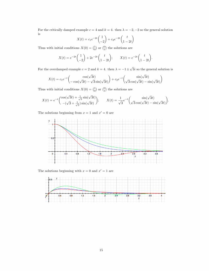
For the critically damped example c = 4 and k = 4. then λ = −2,−2 so the general solutionis

X(t) = c1e−2t(

1

−2

)+ c2e

−2t(

t

1− 2t

)Thus with initial conditions X(0) =

(10

)or(01

)the solutions are

X(t) = e−2t(

1

−2

)+ 2e−2t

(t

1− 2t

); X(t) = e−2t

(t

1− 2t

).

For the overdamped example c = 2 and k = 4. then λ = −1±√

3i so the general solution is

X(t) = c1e−t(

cos(√

3t)

− cos(√

3t)−√

3 sin(√

3t)

)+ c2e

−t(

sin(√

3t)√3 cos(

√3t)− sin(

√3t)

)Thus with initial conditions X(0) =

(10

)or(01

)the solutions are

X(t) = e−t(

cos(√

3t) + 1√3

sin(√

3t)

−(√

3 + 1√3) sin(

√3t)

); X(t) =

1√3e−t(

sin(√

3t)√3 cos(

√3t)− sin(

√3t)

).

The solutions beginning from x = 1 and x′ = 0 are

The solutions beginning with x = 0 and x′ = 1 are

15