Embed Size (px)
Citation preview

Superconformal mattercoupling in three dimensions
and topologically massivegravity
Frederik Lauf
munchen 2019
Superconformal mattercoupling in three dimensions
and topologically massivegravity
Dissertationan der Fakultat fur Physik
der Ludwig-Maximilians-Universitat Munchen
vorgelegt von Frederik Laufaus Bad Sobernheim
Munchen, den 19. August 2019

Erstgutachter: Prof. Dr. Ivo SachsZweitgutachter: Prof. Dr. Peter MayrTag der mundlichen Prufung: 11. Oktober 2019

Zusammenfassung
Die Kopplung supersymmetrischer skalarer Materie-Multipletts an superkonforme Eich-
theorie und Gravitation in drei Raumzeit-Dimensionen wird im Formalismus des N -
erweiterten Superraumes beschrieben. Die Formulierungen supersymmetrischer Eich-
theorie und konformer Supergravitation in diesem Superraum werden vorgestellt und ein
Formalismus fur die Analyse von Superfeldkomponenten wird entwickelt. Ein Superfeld-
Wirkungsprinzip, welches zu einer allgemeinen Klasse minimaler Multipletts auf der
Massenschale fuhrt, wird eingefuhrt. Darauf folgend wird ein Skalar-Multiplett, wel-
ches von einem zwangsbeschrankten Superfeld beschrieben wird und nur aus unter
spin(N ) transformierenden Lorentz-Skalaren und Spinoren besteht, als speziell zwangs-
beschrankter Fall des minimalen unbeschrankten Multipletts identifiziert. Seine Super-
feldwirkung wird aus dem Wirkungsprinzip fur das unbeschrankte skalare Superfeld
hergeleitet. Die Analyse wird fur eine supersymmetrisch eich- und gravitationskovari-
ante Beschreibung von Superfeldkomponenten verallgemeinert und eine Kopplungsbe-
dingung sowie die Wirkung, welche diese Kopplung beschreibt, werden gefunden. Auf
dieser Basis werden alle Eichgruppen fur das Skalar-Multiplett, welche von N ≤ 8 er-
weiterter superkonformer Symmetrie erlaubt sind, im flachen Superraum bestimmt und
ebenso im gekrummten Superraum, in welchem das Skalar-Multiplett zusatzlich gravita-
tionell gekoppelt ist. Dies fuhrt zur Konstruktion samtlicher gravitationell gekoppelter
Chern-Simons-Materie-Theorien. Unter der Benutzung des gravitationell gekoppelten
Skalar-Multipletts als konformen Kompensator werden die resultierenden kosmologi-
schen topologisch massiven Gravitationen nach den korrespondierenden Parametern µ`,
also dem Produkt aus der Kopplungskonstante der konformen Gravitation und dem
anti-de-Sitter-Radius, klassifiziert. Die Modifikationen von µ` bei der Prasenz erlaubter
Eichkopplungen fur den skalaren Kompensator werden bestimmt.
iv
Abstract
The coupling of supersymmetric scalar-matter multiplets to superconformal gauge theory
and gravity in three-dimensional space-time is described in the formalism of N -extended
superspace. The formulations of super-gauge theory and conformal supergravity in this
superspace are reviewed and a formalism for analysing superfield components is devel-
oped. A superfield action principle giving rise to a general class of minimal on-shell
multiplets is introduced. Subsequently, a scalar multiplet described by a constrained su-
perfield and consisting only of Lorentz scalars and spinors transforming under spin(N )
is recognised as a specially constrained case of the minimal unconstrained multiplet.
Its superfield action is deduced from the action principle for the unconstrained scalar
superfield. The analysis is generalised to a super-gauge- and supergravity-covariant de-
scription of superfield components and a coupling condition for the scalar multiplet as
well as the action describing this coupling are obtained. Based on this, all gauge groups
for the scalar multiplet consistent with N ≤ 8 extended superconformal symmetry are
determined in flat superspace, as well as in curved superspace where the scalar multiplet
is also coupled to conformal supergravity. This results in the construction of all super-
conformal Chern-Simons-matter theories coupled to gravity. Using the gravitationally
coupled scalar multiplet as a conformal compensator, the resulting cosmological topolog-
ically massive supergravities are classified with regard to the corresponding parameters
µ`, i.e. the product of the conformal-gravity coupling and the anti-de Sitter radius. The
modifications of µ` in presence of possible gauge couplings for the scalar compensator
are determined.
v


Contents
1. Introduction 1
2. Three-dimensional superspace 9
2.1. Supersymmetry algebra . . . . . . . . . . . . . . . . . . . . . . . . . . . . 10
2.2. Superfields . . . . . . . . . . . . . . . . . . . . . . . . . . . . . . . . . . . 14
2.2.1. Field representation . . . . . . . . . . . . . . . . . . . . . . . . . . 14
2.2.2. Component expansion of superfields . . . . . . . . . . . . . . . . . 16
2.2.3. Supercovariant constraints . . . . . . . . . . . . . . . . . . . . . . 18
2.2.4. Superfield actions and equations of motion . . . . . . . . . . . . . 22
2.2.5. A spin(N ) on-shell superfield . . . . . . . . . . . . . . . . . . . . 24
2.3. Local symmetries . . . . . . . . . . . . . . . . . . . . . . . . . . . . . . . 29
2.3.1. Gauge-covariant derivatives . . . . . . . . . . . . . . . . . . . . . 29
2.3.2. Gauge superalgebra . . . . . . . . . . . . . . . . . . . . . . . . . . 30
2.4. Supergravity . . . . . . . . . . . . . . . . . . . . . . . . . . . . . . . . . . 34
2.4.1. Supergravity-covariant derivative . . . . . . . . . . . . . . . . . . 34
2.4.2. Supergravity algebra . . . . . . . . . . . . . . . . . . . . . . . . . 35
2.4.3. Solution to the constrained Jacobi identity . . . . . . . . . . . . . 38
2.4.4. Super-Weyl invariance . . . . . . . . . . . . . . . . . . . . . . . . 42
2.4.5. Anti-de Sitter superspace . . . . . . . . . . . . . . . . . . . . . . . 43
2.4.6. Conformal superspace . . . . . . . . . . . . . . . . . . . . . . . . 44
3. Coupled scalar matter 49
3.1. Covariant superfield projections . . . . . . . . . . . . . . . . . . . . . . . 50
3.2. Coupled spin(N ) superfield . . . . . . . . . . . . . . . . . . . . . . . . . 51
3.2.1. Gauge-coupled spin(N ) superfield . . . . . . . . . . . . . . . . . . 52
3.2.2. Gravitationally coupled spin(N ) superfield . . . . . . . . . . . . . 53
3.2.3. Gauge- and gravitationally coupled spin(N ) superfield . . . . . . 55
3.3. Matter currents . . . . . . . . . . . . . . . . . . . . . . . . . . . . . . . . 57
3.3.1. Chern-Simons-matter current . . . . . . . . . . . . . . . . . . . . 57
vii

Contents
3.3.2. Supergravity-matter current . . . . . . . . . . . . . . . . . . . . . 59
3.4. All gauge groups for the spin(N ) scalar multiplet . . . . . . . . . . . . . 62
3.4.1. N = 2 (Clifford), N = 3 and N = 4 (chiral) . . . . . . . . . . . . 64
3.4.2. N = 4 (Clifford), N = 5 and N = 6 (chiral) . . . . . . . . . . . . 67
3.4.3. N = 6 (Clifford), N = 7 and N = 8 (chiral) . . . . . . . . . . . . 70
3.5. All gauge groups for the gravitationally coupled spin(N ) scalar multiplet 74
3.5.1. N = 4 . . . . . . . . . . . . . . . . . . . . . . . . . . . . . . . . . 74
3.5.2. N = 5 . . . . . . . . . . . . . . . . . . . . . . . . . . . . . . . . . 75
3.5.3. N = 6 . . . . . . . . . . . . . . . . . . . . . . . . . . . . . . . . . 75
3.5.4. N = 7 . . . . . . . . . . . . . . . . . . . . . . . . . . . . . . . . . 76
3.5.5. N = 8 . . . . . . . . . . . . . . . . . . . . . . . . . . . . . . . . . 80
3.6. Overview of gauge groups . . . . . . . . . . . . . . . . . . . . . . . . . . 84
4. Topologically massive supergravity 87
4.1. Einstein gravity and topologically massive gravity . . . . . . . . . . . . . 87
4.2. Conformal supergravity and conformal compensators . . . . . . . . . . . 90
4.3. Extended topologically massive supergravity . . . . . . . . . . . . . . . . 91
4.3.1. Fixation of µ` . . . . . . . . . . . . . . . . . . . . . . . . . . . . . 91
4.3.2. Gauged compensators . . . . . . . . . . . . . . . . . . . . . . . . 92
5. Conclusion 95
A. Symmetry groups 97
A.1. Fundamental representations . . . . . . . . . . . . . . . . . . . . . . . . . 97
A.2. Index notation . . . . . . . . . . . . . . . . . . . . . . . . . . . . . . . . . 98
A.3. Generators . . . . . . . . . . . . . . . . . . . . . . . . . . . . . . . . . . . 99
A.4. Spin groups . . . . . . . . . . . . . . . . . . . . . . . . . . . . . . . . . . 101
B. Systematic supercovariant projection 105
Bibliography 109
viii

1. Introduction
Fields have been recognised as indispensable entities for the formulation of physical the-
ories since the development of electromagnetism by Maxwell. Today, field theories are
still the language for the most successful models of fundamental phenomena. Incor-
porating the principles of special relativity and quantum mechanics, they describe the
particles and interactions in the Standard Model of particle physics. A classical field
theory for gravity, and thereupon models for cosmology, are implied by the principle of
general relativity.
A particular power for the formulation of field theories is provided by the principle of
symmetry. A symmetry is given, if the most basic description of a theory is invariant
under a specific transformation of its constituting objects.
Above all, the symmetry under space-time transformations is obviously demanded
by the principle of relativity. The symmetry transformations associated to space-time
can act on two kinds of fields which are called bosonic and fermionic. They are the
representations of the space-time symmetry group with integer and half-integer spin,
respectively. Physically, they are conceptually distinguished. The latter describe matter
fields like leptons and quarks, while the former correspond to force particles like photons
and gluons as well as scalar fields like the Higgs boson.
Furthermore, especially in the Standard Model of particle physics, internal symmetry
groups acting on the degrees of freedom formed by the fields themselves play an impor-
tant role. For a manifestly invariant formulation, the degrees of freedom are arranged
in multiplets on which a matrix representation of the respective symmetry group can
act. These transformations become vital if they are allowed to be space-time-dependent.
Such local symmetries, also called gauge symmetries, lead to successful descriptions of
force particles interacting with the matter particles and mediating interactions between
them.
There is no better outside reason for the existence of such internal symmetries, than
that they are, together with space-time symmetry, eligible symmetries of a reasonable
1
1. Introduction
scattering matrix, i.e. the matrix describing scattering processes between particles. In
this regard, there is only one further allowed kind of symmetry. It is called supersym-
metry and concerns the symmetry of space-time itself.
Supersymmetry generalises the symmetry associated to space-time in a way, that the
fermionic and bosonic representations transform into each other. Supersymmetric theo-
ries therefore always describe systems where both kinds of particles appear together and
can be seen as members or aspects, sometimes called superpartners, of one supermul-
tiplet. These supermultiplets can manifestly be described using superfields instead of
fields, which are functions of a superspace instead of space-time, resembling the fact that
supersymmetry is a generalisation of space-time symmetry. The bosonic and fermionic
fields are encapsulated in a superfield as the coefficients of an expansion in even and odd
powers of the fermionic superspace coordinates. Together with supersymmetry comes
another symmetry, similar to an internal one, naturally acting on the fermionic repre-
sentations. These degrees of freedom can be regarded as corresponding to a number Nof usual supersymmetries, implying an extension of the structure of possible supermul-
tiplets. These symmetries are called (N -)extended supersymmetries.
Applying the paradigm of supersymmetry leads to various consequences. As for parti-
cle physics, it would for example predict corresponding superpartners for each particle of
the Standard Model. This has provoked a phenomenological interest in supersymmetry
for decades, with no concluding result so far.
Regarding gravity, the principle of general relativity adapted for superspace leads to
supersymmetric gravity, with the metric field or graviton and a so-called gravitino as
superpartners. An interesting feature of supersymmetry is the automatic implication
of supergravity, if the transformations are local, similar to a gauge theory. After all,
two (fermionic) local supersymmetry transformations correspond to a (bosonic) local
space-time translation, which is the symmetry transformation corresponding to general
relativity.
In this thesis, the focus lies on three-dimensional supersymmetric field theories with
highly extended supersymmetry. Those can be motivated from the point of view of
11-dimensional space-time: The supermultiplet of 11-dimensional N = 1 supersym-
metry contains the graviton as the field with highest spin. Since massless fields with
spins higher than two are considered unphysical, this theory qualifies as the highest di-
mensional and unique supersymmetric field theory and supergravity [1]. The equations
of motion of 11-dimensional (11d) supergravity admit a solution describing spatially
2

two-dimensional membranes which are called M2-branes [2]. Their three-dimensional
world-volume theory [3], i.e. the theory describing their internal dynamics, naturally
involves the coupling to 11d supergravity. The M2-brane world-volume preserves one
half of the 32 supercharges needed to parametrise the N = 1 supersymmetry transfor-
mations in 11 dimensions, thus gaining the higher amount of N = 8 supersymmetry [4],
which is a common effect of this dimensional reduction.
Furthermore, in a suitable scaling limit, the M2-brane solution describes the space
AdS4 × S7 [5], i.e. the four-dimensional space of constant negative curvature with 7-
spheres at each point. In this case, it additionally displays conformal symmetry [6],
which corresponds to invariance under local rescaling of the metric. According to the so-
called AdS/CFT correspondence [6], this suggests the existence of a three-dimensional
superconformal gauge theory with a number of N internal degrees of freedom, which
would be interpreted as the world-volume theory for a stack of N coincident M2-branes.
Another point of view on M2-branes comes from their interplay with superstring
theory. The five known formulations of superstring theory are connected by a web of
dualities, which means they are equivalent ways for describing the same phenomena,
but in different physical regimes. Their low-energy limits are corresponding versions of
ten-dimensional supergravity. One of these, the type IIA supergravity, can directly be
obtained from the unique 11d supergravity, by compactifying one of the 11 dimensions
on a circle whose radius is proportional to the string-coupling constant. Thus, via the
duality web, all ten-dimensional supergravities descend from the 11-dimensional one. In
turn, 11d supergravity is expected to be the low-energy limit of the so-called M-theory,
whose full high-energy formulation is unknown. The superstring theories (as well as 11d
supergravity) are thus regarded as certain limits of M-theory and the M2-branes are
considered as fundamental for M-theory as strings are for string theory.
The type IIA supergravity also contains membranes which are called D2-branes and
describe hypersurfaces for string endpoints. Due to this relation to string dynamics,
the low-energy world-volume theory for a stack of N coincident D2-branes is known to
be a non-conformal three-dimensional gauge theory for N internal degrees of freedom.
The gauge coupling is proportional to the string coupling and thus to the size of the
compactified 11th dimension. Therefore, in the limit of infinite coupling strength, the
size of the 11th dimension increases again, until the theory corresponds to a stack of
M2-branes in 11 dimensions. In this strong-coupling regime, the theory should obtain
the conformal symmetry implied by the AdS/CFT correspondence
The three-dimensional field theory meeting the above requirements for the low-energy
3

1. Introduction
world-volume theory for a stack of M2-branes is N = 8 superconformal Chern-Simons
gauge theory coupled to eight scalar and spinor fields, which are usually called matter
fields [7]. Since the Chern-Simons theory is non-dynamical, the scalar fields represent
the degrees of freedom of M2-branes in the eight transverse directions. The theory is
known as the BLG model [8, 9] and is invariant under the gauge group SU(2)× SU(2).
Due to this unique gauge group, it cannot be interpreted as the world-volume theory of
a stack of N ≥ 2 coincident M2-branes [10, 11], as implied by the D2-brane theory and
desired by the AdS/CFT correspondence. This is however possible for a theory with
only N = 6 supersymmetries and the gauge group SU(N)×SU(N), known as the ABJM
model [12]. The reduction of the amount of supersymmetry is achieved by geometric
restrictions on the transverse coordinates.
Apart from this motivation for the ABJM model, superconformal Chern-Simons-
matter theories with lower amounts N ≤ 8 of supersymmetry and different gauge groups
are still a matter of interest. Their most crucial feature is that possible gauge groups
are restricted by consistency with supersymmetry for N ≥ 4. Notable achievements in
the classification of Chern-Simons-matter theories with regard to supersymmetry and
gauge groups have been made in [13] for N = 4 in the context of four-dimensional su-
persymmetric gauge theories, in [14, 15] for N = 5, 6 in the context of the geometry of
M2-branes, and in demand for formal classifications, in [16] for N = 6 and [17] for all
N . A superspace point of view was adopted in [18] for N = 4, [19] for N = 5, 6, [20] for
N = 6, [21] for N = 6, 8, and in [22] for N = 8.
As a part of the present thesis, this quest is repeated using the formalism of N -
extended superspace. In this approach, the supersymmetric matter is described by a
scalar superfield. The advantage of this approach is not only the manifestly supersym-
metric formulation, but also the as far as possible unified manner in which the cases of
N are analysed. The scalar superfield is subject to a certain supersymmetric constraint
in order to describe a familiar scalar-matter supermultiplet. However, in the presence of
a gauge coupling, this constraint is in general inconsistent. Rather, it is valid only under
an algebraic condition involving a superfield representing the field-strength multiplet,
containing the usual gauge field strength and its superpartners. In general, these field
strengths have to be expressed by the scalar-matter current which couples to the gauge
fields, according to their Chern-Simons equation of motion. The specific algebraic prop-
erties of these matter currents decide on the solvability of the condition for the scalar
superfield and thus over the admissibility of the gauge group in question.
4

The classification of coupled supersymmetric matter gives rise to another application,
which is the realisation of certain supergravity theories. Non-supersymmetric three-
dimensional gravity, likewise a field theory emerging in curved space, has some distin-
guished features compared to its analogue in four dimensions. Namely, both its versions
of Einstein-Hilbert gravity and conformal gravity each for themselves have no dynamics.
The latter is solved by conformally flat space-time and the former completely fixes the
geometry of space-time by its equations of motion to be flat or have constant curvature,
leaving no room for a locally propagating graviton. Nevertheless, in the presence of a
negative cosmological constant, a black hole solution [23] with anti-de Sitter space as
the asymptotic limit and in consequence [24] a corresponding two-dimensional conformal
field theory in this region with its two propagating modes are supported.
Thanks to the existence of these two models for gravity, a third model can be con-
structed by adding them together. The result is a dynamical theory known as topologi-
cally massive gravity [25], since it gives rise to a new propagating degree of freedom with
a mass determined by the coupling of the conformal supergravity. It notoriously requires
some finesse regarding the positivity of the occurring energies. As for the massive gravi-
ton alone and in absence of the cosmological constant, the sign of the Einstein-Hilbert
action must be inverted to ensure a positive energy. This carries with it the downside
of negative black-hole masses upon including the negative cosmological constant. A
sensible model with no negative energies is given by the so-called chiral gravity [26]. It
is characterised by the usual sign of the Einstein-Hilbert action and the value µ` = 1,
where µ is the conformal-gravity coupling and ` is the anti-de Sitter radius related to the
negative cosmological constant. Under this specification, the black holes have positive
mass while the massive graviton and one of the boundary gravitons disappear, leaving
only one mode with positive energy in the boundary conformal field theory [27].
N -extended supergravity in three dimensions can be formulated inN -extended curved
superspace. This approach automatically leads to a description of conformal super-
gravity. In view of the Einstein-Hilbert term of topologically massive gravity, realising
non-conformal supergravities requires the coupling to certain fields which are called
conformal compensator. These have to display specific properties in order to ensure
conformal invariance. In a second step, the conformal symmetry can be broken by fixing
an expectation value of the compensator, thus preventing it from preserving conformal
invariance by compensating for the transformations of the other fields in the theory.
5

1. Introduction
In order to serve as a conformal compensator, the scalar-matter multiplet coupled to
superconformal Chern-Simons theories can further be coupled to conformal supergravity
[28, 29, 21]. This carries with it the effect of modifying the spectrum of the admissi-
ble gauge groups compared to flat superspace [30, 21]. The above superfield formalism
for the coupled scalar-matter multiplet remains applicable, but in addition to the field-
strength multiplet, there appears the conformal-supergravity multiplet described by a
superfield called super-Cotton tensor. It contains the Cotton tensor, which is an in-
variant tensor of conformal gravity constructed from the curvature tensor, but instead
of curvature, it measures the conformal flatness of a space-time. The impact of curved
superspace on the allowed gauge groups is quite particular regarding the number of su-
persymmetries. In the cases N = 4 and N = 5 it has no effect. For N = 6, it relaxes
the restrictions on certain U(1) factors of the gauge groups present in flat superspace
[30]. This phenomenon is due to the fact, that the N = 6 super-Cotton tensor can be
regarded as being dual to a U(1) field strength. For N = 7 and N = 8 it gives rise to
the possibility of matter fields in the fundamental representations of gauge groups which
are unrelated to those in flat superspace.
Using the gauge- and supergravity-coupled scalar-matter multiplet as a conformal
compensator naturally realises supersymmetric versions of topologically massive grav-
ity. A distinguished feature of the resulting theories is that the value of µ` is always
fixed by the superconformal geometry for N ≥ 4 [31, 32]. The underlying mechanism
is essentially the following. Since the super-Cotton tensor contains the field strength
of the gauged SO(N ) structure group of extended superspace, its value is determined
by the Chern-Simons coupling µ via the Chern-Simons equation of motion of confor-
mal supergravity. In the geometry defining anti-de Sitter superspace, the cosmological
constant is generated by the value of a torsion superfield transforming inhomogeneously
under super-Weyl transformations, which are transformations related to conformal in-
variance. The presence of a scalar compensator superfield in this background requires a
gauge for this superfield relating it to the super-Cotton tensor. Upon giving the scalar
compensator its expectation value, this fixes the relation between µ and `.
As is the nature of a conformal compensator, the opposite sign of the Einstein-Hilbert
action is generated [29]. It suggests that the nature of negative mass BTZ black holes,
being a consequence of this sign, should be addressed by different interpretations. This
issue is not a topic of this thesis, but will be addressed again in the conclusion.
The question is then which supergravities may imply the value µ` = 1 preferred by
6

the model of chiral gravity. They are the ones with N = 4 [31] and N = 6 [29]. The list
of values µ` for all amounts of supersymmetry 4 ≤ N ≤ 8 obtained from the analysis
with a compensator not coupled to a gauge group is [32]
N = 4 5 6 7 8
(µ`)−1 = 1 3/5 1 2 3 .
Modifications of these values may occur if the compensator is also coupled to its allowed
gauge groups [21, 32]. In this case, a number of its gauge components can be chosen to
generate the Einstein-Hilbert coupling constant. The most diverse, yet specific, effects
appear for N = 6 with gauge group SU(N) in shape of the formula [32]
(µ`)−1 =2
p− 1,
where p is the number of non-vanishing components, and for N = 8 with the gauge
group SO(N) [21] and the formula [33]
(µ`)−1 =4
p− 1.
Both cases additionally allow µ` =∞ corresponding to the solution of Minkowski space.
For N = 8 also the value µ` = 1 can be generated by choosing two compensator com-
ponents.
Outline. The present thesis is organised as follows. In Chapter 2, the formalism of
three-dimensional extended superspace is introduced to describe supersymmetric scalar
matter fields, super-gauge theory and conformal supergravity, which will be coupled
together in the subsequent Chapter 3. Regarding supersymmetric scalar matter, the
component expansion of scalar superfields is developed and discussed, with the goal of
arriving at the case of an on-shell multiplet described by a constrained superfield, which
consists of a scalar and a spinor field transforming under the fundamental representation
of spin(N ). An off-shell superfield action principle leading to a general class of minimal
on-shell multiplets is proposed, from which the spin(N ) scalar multiplet and its superfield
and component actions follow as a special, constrained case. Subsequently, super-gauge
theory and conformal supergravity in the formulations of conventional curved SO(N )
7

1. Introduction
superspace and conformal superspace are reviewed. A special focus lies on anti-de Sit-
ter superspace as a supersymmetric background solution of supergravity, which will be
relevant for topologically massive supergravity discussed in Chapter 4.
In Chapter 3, the component analysis of scalar superfields is generalised in order
to describe gauge-covariant superfield components. This leads to the derivation of a
coupling condition for the spin(N ) scalar multiplet, which is implied by consistency with
the covariant constraint on the scalar superfield describing this multiplet or, in other
words, by consistency of the supersymmetry transformations of its covariant components.
This condition is then fully analysed and solved for 4 ≤ N ≤ 8, resulting in the complete
spectrum of allowed gauge groups in flat as well as in curved superspace. To this end, the
scalar-matter currents which couple to gauge fields are determined and recast as scalar-
superfield currents, corresponding to equations of motion for the superfields describing
the gauge and supergravity multiplets.
In Chapter 4, results are combined in order to use the coupled scalar multiplet as
a conformal-compensator multiplet for topologically massive supergravities. Requiring
consistency with the background of anti-de Sitter superspace leads to a formula for the
values of µ` with a single compensator, depending on the case N . Subsequently, the
effects on the value of µ` generated by a gauged scalar compensator will be investigated.
Aspects and conventions of the general treatment of symmetry groups used in the
main text, as well as some formal expressions belonging to the superfield-component
analysis have been relegated to the appendix.
8

2. Three-dimensional superspace
In this chapter, the relevant formalisms in three-dimensional superspace needed for the
later purpose of coupling supersymmetric scalar matter conformally to super-gauge the-
ory and conformal supergravity are reviewed, developed, or elaborated on.
In Section (2.1), the supersymmetry algebra is introduced and properties of the
Lorentz group are presented.
In Section (2.2), the representation of supersymmetry on superfields is discussed and
a formalism for the analysis of superfield components is developed. An off-shell action
principle, giving on shell rise to minimal scalar multiplets, is proposed. Based on this
formalism, the constrained scalar superfield transforming under spin(N ) describing the
on-shell multiplet coupled to super-gauge fields and supergravity in the next chapter is
analysed and the corresponding superfield action is derived.
In Section (2.3), gauge-covariant derivatives are introduced and the content of the
gauge connection is examined. The algebra of covariant derivatives is derived by solving
the super-Jacobi identity under the constraint defining the field-strength multiplet.
In Section (2.4), two descriptions of extended conformal supergravity are presented.
The first approach is the conventional curved SO(N ) superspace, which is described by
certain Weyl-invariant constraints on the torsions. These will be motivated by investigat-
ing the algebra of covariant derivatives in terms of the gauge fields of the local structure
group. The super-Jacobi identity will be solved under these constraints in order to de-
rive the field strengths in the supergravity algebra in terms of the super-Cotton tensor
and the torsions. Subsequently, anti-de Sitter superspace is introduced as the maximally
symmetric background of this geometry. The more briefly presented second approach
is conformal superspace, where the whole superconformal group is gauged as the local
structure group. It can be translated into conventional superspace and is convenient for
obtaining useful relations in a simpler way.
9

2. Three-dimensional superspace
2.1. Supersymmetry algebra
Three-dimensional supersymmetric space-time or superspace is parametrised by the co-
ordinates
zA = (xa, θIα), (2.1.1)
where θIα are odd supernumbers, i.e.
θαI θβJ = −θβJθ
αI , (2.1.2)
carrying an SL(2,R) index α = 1, 2 and an SO(N ) index I = 1, ...,N . The space-time
coordinate xa carries an SO(2, 1) index a = 0, 1, 2.
The symmetry group of this superspace is the three-dimensional super-Poincare group,
which is generated by the super-Poincare algebra. The super-Poincare algebra is ob-
tained from the Poincare superalgebra
[M ab,M cd] = −4η[c[aM b]d] (2.1.3a)
[Pa, Pb] = 0 (2.1.3b)
QIα, Q
Jβ = 2δIJPαβ (2.1.3c)
by requiring anticommuting parameters for the fermionic generators QIα and commuting
parameters for the remaining bosonic generators. In other words, an element of the
super-Poincare algebra reads
X = 12ωabMab + iaaPa + iεαIQ
Iα, (2.1.4)
where
εαI εβJ = −εβJε
αI . (2.1.5)
The part corresponding to the bosonic part of the Poincare superalgebra is the symme-
try group of non-supersymmetric space-time SO(2, 1) oR3. The part corresponding to
the fermionic part is the group of supersymmetry transformations.
Referring to the terminology introduced in Appendix A, the Lorentz group SO(2, 1)
is the pseudo-orthogonal group with
ηmn = diag(−1, 1, 1)mn (2.1.6)
10

2.1. Supersymmetry algebra
and SL(2,R) is the symplectic group Sp(2) with
εαβ =
(0 1
−1 0
)αβ
. (2.1.7)
The two-to-one correspondence between these two groups is established by mapping
a Lorentz vector to the space of symmetric 2 × 2-matrices Sym(2,R) with the basis
Sm = S0, S1, S2, where
S0 =
(1 0
0 1
), S1 =
(0 1
1 0
), S2 =
(1 0
0 −1
). (2.1.8)
This basis is (pseudo-) normalised as
tr(SmSn) = −2ηmn, (2.1.9)
where Sm = S0,−S1,−S2. The components of a Lorentz vector xm are the expansion
coefficients in this basis,
X = xmSm, (2.1.10)
and inversely,
− 12tr(XSm) = −1
2tr(xnS
nSm) = xm. (2.1.11)
Since the negative determinant of X equals the scalar product of the Lorentz vector, a
Lorentz transformation of X must be determinant- and symmetricity-preserving, i.e.
XLT−→ X = AXAT (2.1.12)
with A ∈ SL(2,R) being an element of the group of 2×2-matrices with unit determinant.
The map between A ∈ SL(2,R) and Λ ∈ SO(2, 1) follows from
−12tr(XSm) = xm (2.1.13)
as
−12tr(ASnA
TSm) = Λmn. (2.1.14)
11
2. Three-dimensional superspace
It is a two-to-one map because A and −A are mapped to the same Λ. In other words,
SO(2, 1) ∼= SL(2,R)/Z2. (2.1.15)
As is apparent, the matrices Sm have two lower indices and the matrices Sm have two
upper indices,
(Sm)αβ = εαγεβδ(Sm)γδ. (2.1.16)
A set with one lower and one upper index is defined by
(γ0) βα ≡− εβγ(S0)αγ
(γ1,2) βα ≡εβγ(S1,2)αγ. (2.1.17)
These are a basis for traceless matrices and fulfil the Clifford algebra
γm,γn = 2ηmn. (2.1.18)
In this context of space-time symmetry, the components of SL(2,R) vectors (also called
spinors) are odd supernumbers with
vαwβ = −wβvα (2.1.19)
and the complex conjugation rule
(vαwβ)∗ = w∗βv∗α. (2.1.20)
An antisymmetric SO(2, 1) tensor of rank two, a vector and a rank-two SL(2,R) tensor
are equivalent to each other by the relations
Fab = εabcFc = εabc(−1
2εcdfFdf ) (2.1.21a)
Fαβ = (γa)αβFa = (γa)αβ(−12(γa)
γδFγδ). (2.1.21b)
The contraction of two Lorentz vectors can thus be written in the forms
F aGa = −12F abGab = −1
2FαβGαβ. (2.1.22)
12
2.1. Supersymmetry algebra
The action of the Lorentz generators with different label representations is given by
M abvc = 2ηc[avb] (2.1.23a)
M avb = −εabcvc (2.1.23b)
M αβvc = −(γcb)αβvb (2.1.23c)
and
M abvγ = 12(γab) δ
γ vδ (2.1.24a)
M avγ = 12(γa) δ
γ vδ (2.1.24b)
M αβvγ = εγ(αvβ) (2.1.24c)
for Lorentz vectors and spinors, respectively. The commutation relation can be written
in the forms
[M ab,M cd] = −4η[c[aM b]d] (2.1.25a)
[M a,M b] = εabcMc (2.1.25b)
[Mαβ,Mγδ] = −2ε(γ(αMβ)δ). (2.1.25c)
13

2. Three-dimensional superspace
2.2. Superfields
2.2.1. Field representation
Fields A(x, θ) in superspace are covariant with the coordinates both as finite- and
infinite-dimensional representations of the super-Poincare group. The former correspond
to transformations in a finite vector space representing SL(2,R)
A′(x′, θ′) = A(x, θ) + δA(x, θ) = A(x, θ) + 12ωabM f
ab ·A(x, θ) (2.2.1)
and the latter to translations in the infinite space of functions
A′(x, θ) = A(x, θ) + ∆A(x, θ). (2.2.2)
In this infinitesimal form, the two are related by a Taylor expansion
∆A(x, θ) = δA(x, θ)− (aa + ωabxb)∂aA(x, θ)
− (εαI + 14ωab(γab)
αβθβI)∂IαA(x, θ), (2.2.3)
where ∂a ≡ ∂∂xa
and ∂Iα ≡ ∂∂θαI
. Comparing the commutator
[∆1,∆2] =ωac1 ωb
2c (M fab + 2x[a∂b] − 1
4(γab)
αβθβI∂Iα)
+ 2ab[1ωbc2]∂c + 2εαI[1 (∂Iαa
a2])∂a (2.2.4)
with the one of two generators X = 12ωabMab + iaaPa + iεαIQ
Iα,
[X1, X2] =ωac1 ωb
2c Mab + i2ωab[1 ε
αI2] (γab)
βα QβI − 2iaa[1ω
b2]a Pb + 2εαI1 εβ2IPαβ, (2.2.5)
reveals that aa must have the θ-dependent part, or the “soul”
aSa = −iεαIθβI (γa)αβ, (2.2.6)
while
Mab =M fab + 2x[a∂b] − 1
4(γab)
αβθβI∂Iα (2.2.7a)
Pa =i∂a (2.2.7b)
QIα =i∂Iα + θβI(γa)αβ∂a. (2.2.7c)
14
2.2. Superfields
Furthermore, there is a supercovariant derivative
DIα = ∂Iα + iθβI(γa)αβ∂a (2.2.8)
commuting with the supersymmetry generator,
DIαε
βJQ
JβA = εβJQ
JβD
IαA, (2.2.9)
and obeying the supersymmetry algebra
DIα, D
Jβ = 2iδIJ∂αβ. (2.2.10)
It has the useful property [34]
(DIαA)∗ =−DI
αA∗ (2.2.11a)
(DIαAβ)∗ =DI
αA∗β (2.2.11b)
and likewise for all SL(2,R) tensors of even or odd rank.
It can be convenient to combine the supercovariant spinor derivative together with
the vector derivative ∂a ≡ Da into a supervector
DA = (Da, DIα). (2.2.12)
It is subject to the algebra
[DA, DB ≡ DADB − (−1)ABDBDA = TCABDC , (2.2.13)
where the powers A are 0 if A is a vector index and 1 if it is a spinor index. The torsion
TCAB is constrained by
T cαβ = 2i(γc)αβ, (2.2.14)
while all others are zero.
15
2. Three-dimensional superspace
2.2.2. Component expansion of superfields
A superfield is expanded in powers of θIα as
A(x, θ) = a(x) + θαI aIα(x) + 1
2θαI θ
βJa
JIβα(x) + ... . (2.2.15)
The component fields are give by the projections
(∂I1α1...∂IkαkA)|θ=0 ≡ ∂I1α1
...∂IkαkA| ≡ aI1...Ikα1...αk. (2.2.16)
This definition requires appropriate normalisation factors in the explicit expansion as
indicated above. Since the spinor derivatives anti-commute, the component fields have
the symmetry property
aI1...IiIj ...Ikα1...αiαj ...αk= −aI1...IjIi...Ikα1...αjαi...αk
. (2.2.17)
Supercovariant projections are denoted by
DI1α1...DIk
αkA| ≡ AI1...Ikα1...αk
. (2.2.18)
They are related to the component fields by
AI1...Ikα1...αk= aI1...Ikα1...αk
+ AI1...Ikα1...αk
. (2.2.19)
The fields AI1...Ikα1...αk
depend on multiple space-time derivatives of components of corre-
spondingly lower ranks. Explicitly, they are given by
AIα =0 (2.2.20a)
AIJαβ =iδIJ∂αβa (2.2.20b)
AIJKαβγ =iδJK∂βγa
Iα − iδIK∂αγa
Jβ + iδIJ∂αβa
Kγ (2.2.20c)
AIJKLαβγδ =iδIJ∂αβa
KLγδ − iδIK∂αγa
JLβδ + iδKL∂γδa
IJαβ
+ iδIL∂αδaJKβγ + iδJK∂βγa
ILαδ − iδJL∂βδa
IKαγ
− δIJδKL∂αβ∂γδa+ δIKδJL∂αγ∂βδa− δILδJK∂αδ∂βγa, (2.2.20d)
and so on. Systematic formulas and further examples are presented in Appendix B.
In the following, this relation will be symbolically denoted by
AI1...Ikα1...αk= aI1...Ikα1...αk
+ AI1...Ikα1...αk
(∂a(−2), ∂∂a(−4), ...), (2.2.21)
16

2.2. Superfields
where a(−l) is of rank k − l.
Under infinitesimal supersymmetry transformations, the superfield changes by
δεA = iεαIQαIA = εαI(−DIα + 2iθIβ∂αβ)A. (2.2.22)
The transformed components are the components of the transformed superfield, i.e.
δaI1...Ikα1...αk= ∂I1α1
...∂IkαkδA| = DI1α1...DIk
αkδA| − AI1...Ik
α1...αk(∂δa(−2), ∂∂δa(−4), ...). (2.2.23)
Re-expressing the supercovariant projections, it follows
δaI1...Ikα1...αk= −εαIaII1...Ikαα1...αk
− εαIAII1...Ikαα1...αk
(∂a(−2), ...)− AI1...Ikα1...αk
(∂δa(−2), ...), (2.2.24)
iteratively describing the transformations of all superfield components.
It can be shown that these transformations indeed represent the supersymmetry alge-
bra by considering two successive transformations
δηδεaI1..Ikα1..αk
=εαI ηβJa
JII1..Ikβαα1..αk
+ εαI ηβJA
JII1..Ikβαα1..αk
(∂a(−2), ..)− AI1..Ikα1..αk
(∂δηδεa(−2), ..). (2.2.25)
Their commutator is
[δη, δε]aI1..Ikα1..αk
=(εαI ηβJ − η
αI ε
βJ)AJII1..Ik
βαα1..αk(∂a(−2), ..)− AI1..Ik
α1..αk(∂[δη, δε]a(−2), ..). (2.2.26)
The combination of the parameters on the right-hand side is either symmetric or anti-
symmetric in both types of indices projecting on the corresponding representations in
AJII1...Ikβαα1...αk
. This is only the symmetric one, given by
AI1I2...Ikα1α2...αk
+ AI2I1...Ikα2α1...αk
= 2iδI1I2∂α1α2aI3...Ikα3...αk
+ 2iδI1I2∂α1α2AI3...Ikα3...αk
, (2.2.27)
as is apparent from its definition. Assuming that the supersymmetry algebra closes on
fields of lower ranks inductively leads to its closure on all components,
[δη, δε]aI1...Ikα1...αk
=2iεαI ηβJδ
IJ∂αβaI1...Ikα1...αk
. (2.2.28)
It is difficult to read off an explicit solution from the inductive transformation formula.
17

2. Three-dimensional superspace
For example, the transformations of the first five components read
δa =− εαI aIα (2.2.29a)
δaIα =− εβJaJIβα − iεβJδ
JI∂βαa (2.2.29b)
δaJIβα =− εγKaKJIγβα − iεγK(−δKI∂γαaJβ + δKJ∂γβa
Iα) (2.2.29c)
δaKJIγβα =− εδLaLKJIδγβα − iεδL(δLK∂δγaJIβα − δLJ∂δβaKIγα + δLI∂δαa
KJγβ ) (2.2.29d)
δaLKJIδγβα =− εεMaMLKJIεδγβα (2.2.29e)
− iεεM(δML∂εδaKJIγβα − δMK∂εγa
LJIδβα + δMJ∂εβa
LKIδγα − δMI∂εαa
LKJδγβ ).
Apparently, each component transforms into the next higher component and first deriva-
tives of the next lower component. Terms with more derivatives drop out and would be
inconsistent with the symmetry of the tensor on the left-hand side. Therefore, it can be
concluded that
δaIk...I1αk...α1=− εαk+1
Ik+1
(aIk+1...I1αk+1...α1
+ iδIk+1Ik∂αk+1αkaIk−1...I1αk−1...α1
), (2.2.30)
where the brackets . collect the sum of k terms sharing the symmetry of the tensor
on the left-hand side, as in the above examples.
The transformation of irreducible SL(2,R)× SO(N ) representations contained in the
components can easily be derived from the above formula. The particularly common
partially reduced field(n)a αk...α1 defined by
(n)a Ik...I1
αk...α1= (−1
2)nδJ1J2ε
β1β2 ...δJ2n−1J2nεβ2n−1β2naIk...I1J2n...J1αk...α1β2n...β1
(2.2.31)
has the transformation
δ(n)a Ik...I1
αk..α1=− εαk+1
Ik+1
(aIk+1...I1αk+1..α1
+ iδIk+1Ik∂αk+1αkaIk−1...I1αk−1..α1 − in(−1)k∂ β
αk+1
(n−1)a
Ik...I1Ik+1
αk..α1β
).
(2.2.32)
2.2.3. Supercovariant constraints
Since the supercovariant derivatives commute with supersymmetry transformations, they
can be used to impose supersymmetrically invariant constraints on superfields. In view of
the later purpose of describing scalar multiplets, an important class of scalar constraint
18
2.2. Superfields
equations considered in the following is
(DαID
Iα)nA ≡ (D2)nA ≡
(n)
A= 0. (2.2.33)
Hiding the SO(N ) indices, the components of this superfield equation are
(n)
A | =(n)a +
(n)
A= 0 (2.2.34a)
∂β1(n)
A | =(n)
A β1=(n)a β1 +
(n)
A β1= 0 (2.2.34b)
...
∂β2N−2n..∂β1
(n)
A | =(n)a β2N−2n..β1 +
(n)
A β2N−2n..β1= 0 (2.2.34c)
∂β2N−2n+1..∂β1
(n)
A | =(n)
A β2N−2n+1..β1= 0 (2.2.34d)
...
∂β2N ..∂β1(n)
A | =(n)
A β2N ..β1= 0, (2.2.34e)
where components of A being determined by lower components of the equation have to
be accordingly substituted in the higher components. This is why the spinor derivatives
∂Iα on the left-hand-sides can be replaced by supercovariant derivatives.
The equations of the form(n)a βk..β1= −
(n)
A βk..β1 (2.2.35)
determine the components(n)a βk..β1 in terms of derivatives of lower components; however,
the equations(n)
A β2N−2n+l..β1= 0 (2.2.36)
give rise to higher-order differential relations among the lower components and other
representations(m<n)a βl..β1 . This circumstance shows that the constraint sets the super-
field partially on shell.
The constraint is invariant under the transformation
A −→ A−B, (2.2.37)
if(m≤n−1)
B = 0. (2.2.38)
19

2. Three-dimensional superspace
This gauge freedom can be fixed in the superfield A defined by
A = A+B|A, (2.2.39)
where B|A means that the component fields appearing in the constrained superfield
B are evaluated at the values of the components of A. Concretely, A a has those
components gauged away which are unconstrained in B and the other components are
redefined in terms of the constrained components of B and are not redundant.
In order to illustrate the above in an example, one can consider the case N = 2 and
D2D2A = 0. (2.2.40)
This constraint is invariant under
A −→ A−B, (2.2.41)
where
D2B = 0. (2.2.42)
The components of B fulfil
b =0 (2.2.43a)
bIα =− BIα = i∂ µ
α bIµ (2.2.43b)
bJIβα =− BJIβα = εβαδ
JIb− 2i∂ µ(β b
[IJ ]α)µ (2.2.43c)
0 = ˜BKγ = 0 (2.2.43d)
0 = ˜BLKδγ = ∂ µ
γ ∂ ν(δ b
[KL]µ)ν (2.2.43e)
20

2.2. Superfields
and the gauge shift translates to the components of A as
a −→ a− b (2.2.44a)
aIα −→ aIα − bIα (2.2.44b)
a −→ a (2.2.44c)
a((JI)) −→ a((JI)) − b((JI)) (2.2.44d)
a[JI](βα) −→ a
[JI](βα) − b
[JI](βα)
∣∣0=∂ β
γ ∂ α(δ
b[IJ]β)α
(2.2.44e)
aIα −→ aIα − i∂ µα bIµ (2.2.44f)
aJIβα −→ aJIβα − εβαδJIb− 2i∂ µ(β b
[IJ ]α)µ , (2.2.44g)
where a((JI)) denotes the traceless part of −12εαβa
(JI)βα . The fields a, aIα and a((JI)) can be
shifted arbitrarily and possibly to zero, while the fields a, aIα and aJIβα are non-redundant.
Being interested in a minimal non-redundant multiplet, the field a[JI](βα) can further be
required to fulfil the constraint
0 = ∂ βγ ∂ α
(δ a[IJ ]β)α , (2.2.45)
in which case it can be shifted to zero as well.
According to (2.2.39), the components of A are then redefined as
a = a (2.2.46a)
aIα = aIα (2.2.46b)
a = ˆa (2.2.46c)
a((IJ)) = a((IJ)) (2.2.46d)
a[JI](βα) = a
[JI](βα) (2.2.46e)
aIα = ˆaIα + i∂ µα aIµ (2.2.46f)
aJIβα = ˆaJIβα + εβαδJIa+ 2i∂ µ
(β a[IJ ]α)µ . (2.2.46g)
The gauge-fixed superfield A is therefore given by
A = 12θαI θ
Iα(ˆa+ θγK
ˆaKγ + 12θγKθ
δLˆaKLδγ ). (2.2.47)
Due to (2.2.46g) and the condition (2.2.45), the Lorentz vector ˆa[KL](δγ) has to fulfil the
same relation as the vector ∂ µ(β a
[IJ ]α)µ in (2.2.45). This can be written as the Maxwell
21
2. Three-dimensional superspace
equation and Bianchi identity
∂ γ(α
ˆa[KL]δ)γ = ∂γδ ˆa
[KL]δγ = 0. (2.2.48)
In summary, the superfields A and A fulfil the same constraint equation
D2D2A = D2D2A = 0 (2.2.49)
under the assumption of (2.2.48).
2.2.4. Superfield actions and equations of motion
A generalisation of the action known from N = 1 supersymmetry [35] is
S =
∫d3x (d2θ)N (Dα1
I1..DαN
INA)DI1
α1..DIN
αNA|. (2.2.50)
It is manifestly invariant under supersymmetry, since the integral is over the whole
superspace, i.e. the spinorial measure (d2θ)N ≡ (∂αI ∂Iα)N contains all spinor derivatives
and is thus annihilated by every supersymmetry generator. It is worth to note that
(∂αI ∂Iα)N may be replaced by (Dα
IDIα)N up to a total derivative, which is useful for
obtaining the component action. While the choice of the measure is unique (assuming
that no indices are contracted with those of the integrand), the integrand is highly
reducible. A particular choice in view of the present purpose is the completely traced
part. For even N it is
S =
∫d3x (d2θ)N [(D2)nA](D2)nA| (2.2.51)
and for odd NS =
∫d3x (d2θ)N [Dα
I (D2)nA]DIα(D2)nA|, (2.2.52)
where n = N2
or n = N−12
respectively.
The superfield equation of motion can be obtained by partially integrating so that
S =
∫d3x (d2θ)N A(D2)NA|, (2.2.53)
22

2.2. Superfields
and is given by
(D2)NA = 0. (2.2.54)
It is of the constraint form studied above. It has a redundancy due to the transformation
A −→ A−B, (2.2.55)
where
(D2)N−1B = 0. (2.2.56)
Written in components (2.2.34), and omitting the SO(N ) indices, this constraint on B
reads
(N−1)
B | =(N−1)
b +(N−1)
B = 0 (2.2.57a)
∂β1(N−1)
B | =(N−1)
B β1=(N−1)
b β1 +(N−1)
B β1= 0 (2.2.57b)
∂β2∂β1(N−1)
B | =(N−1)
b β2β1 +(N−1)
B β2β1= 0 (2.2.57c)
∂β3 ..∂β1(N−1)
B | =(N−1)
B β3..β1= 0 (2.2.57d)
...
∂β2N ..∂β1(N−1)
B | =(N−1)
B β2N ..β1= 0. (2.2.57e)
Accordingly, the components(N−1)a ,
(N−1)a I
α and(N−1)a JI
βα are not redundant, but can be
redefined to invariant fieldsˆ(N−1)a ,
ˆ(N−1)a I
α andˆ(N−1)a JI
βα as defined by (2.2.39). The other
components can be gauged away if they fulfil the superfield equation of motion, because
in this case they fulfil the same differential relations as the corresponding components
of the gauge parameter field B.
In consequence, the superfield equation of motion contains the non-redundant infor-
mation
ˆ(N )a = 0 (2.2.58a)
N i∂ µα
ˆ(N−1)a I
µ = 0 (2.2.58b)
−iN∂ µ(β
ˆ(N−1)a [IJ ]
α)µ + δJIεβαˆ(N−1)a = 0. (2.2.58c)
This system contains the equations of motion of a minimal on-shell multiplet, being
23

2. Three-dimensional superspace
defined by the above off-shell action. The Lorentz vectorˆ(N−1)a JI
βα, even though it appears
quadratic in the off-shell action, on shell fulfils the Maxwell equation and in addition
the Bianchi identity, which is an effect of the on-shell gauge fixing as demonstrated for
the example (2.2.48).
2.2.5. A spin(N ) on-shell superfield
A superfield Qi transforming under the fundamental representation of spin(N ) (see
Appendix A) can be subject to the constraint [31, 22, 20, 18, 19]
DIαQi = (γI) ji Qjα, (2.2.59)
where Qiα is a general superfield carrying an additional Lorentz index and reads
Qiα = qiα + θβJqJ
iα,β + ... . (2.2.60)
For chiral representations of spin(N ), the constraint is
DIαQ = Σ IQα (2.2.61)
or
DIαQ = Σ IQα, (2.2.62)
depending on the chosen handedness. The chiral spin(N ) indices have been omitted,
since they depend on the specific case of N . A discussion of fields transforming under
chiral representations will follow in Chapter 3. In the following formal considerations,
the form for non-chiral representations will be used.
The first component of the constraint superfield equation is
qIα = γIqα. (2.2.63)
Taking a general number of supercovariant projections
QJk..J1Iβk..β1α
= γIQ Jk..J1α,βk..β1
(2.2.64)
24
2.2. Superfields
and reminding that
QIk..I1αk..α1
= qIk..I1αk..α1+ QIk..I1
αk..α1, (2.2.65)
leads to the expression for the components of Qi
qJk..J1Iβk..β1α= γIq Jk..J1
α,βk..β1+ γIQ Jk..J1
α,βk..β1−QJk..J1I
βk..β1α(2.2.66)
in terms of the components of Qiα. These are determined by taking the representations
of this equation not contained in qJk..J1Iβk..β1α, i.e. both symmetric or antisymmetric in a
particular index pair, leading to
QJk..(J1I)βk..(β1α) − γ
(IQ|Jk..|J1)
(α,|βk..|β1) =γ(Iq|Jk..|J1)
(α,|βk..|β1) (2.2.67a)
QJk..[J1I]βk..[β1α] − γ
[IQ|Jk..|J1]
[α,|βk..|β1] =γ[Iq|Jk..|J1]
[α,|βk..|β1]. (2.2.67b)
In terms of covariant projections, this is solved by
QJk..J1
(α,|βk..|β1) =i∂β1αγJ1QJk..J2
βk..β2+ ... (2.2.68a)
QJk..J1
[α,|βk..|β1] =0, (2.2.68b)
where the dots indicate the further permutations implied by the symmetries on the
left-hand-side (an example will appear below). Accordingly, the components or super-
covariant projections of Qi are provided by the expressions
QJk..[J1I]βk..(β1α) =i∂β1αγ
IJ1QJk..J2βk..β2
+ ... (2.2.69a)
QJk..(J1I)βk..[β1α] =0. (2.2.69b)
For the second component this means
q[JI](βα) =iγIJ∂βαq (2.2.70a)
q(JI) =0. (2.2.70b)
The constraint (2.2.59) therefore defines an on-shell multiplet consisting of q and qα,
subject to the supersymmetry transformations
δq =− εαI γIqα (2.2.71a)
δqα =− iεβJγJ∂βαq. (2.2.71b)
25

2. Three-dimensional superspace
This multiplet corresponds to the special case of a minimal on-shell multiplet (2.2.58)
arising from an unconstrained scalar superfield with an attached spin(N ) index, where
(N )a = 0 (2.2.72a)
(N−1)a I
α = γIqα (2.2.72b)
(N−1)a [JI]
(βα) = iγIJ∂βαq. (2.2.72c)
In other words, the defining constraint (2.2.59) for Qi removes the vector(N−1)a [JI]
(βα) by
identifying it with the derivative of the scalar field, which is consistent with the Maxwell
equation and the Bianchi identity fulfilled by this vector.
Since the scalar multiplet is encoded in the lowest components of the constrained
superfield Qi, a corresponding superfield action resembles the one for N = 1 [35]. It
may be postulated as
S = 1A(N )
∫d3x dθαI dθIα (Dγ
KQ)DKγ Q|
= 1A(N )
∫d3x (Qγ
KQαIKIαγ −Q
αIγIαKQ
Kγ − 2Qαγ
IKQIKαγ ), (2.2.73)
where A(N ) is a normalisation factor. Indeed, reminding that
QγβαKJI =iγIγJγK∂
αβqγ + iγJγKγI∂γβqα − iγIγKγJ∂
γαqβ (2.2.74a)
QβαJI =iγIγJ∂
αβq, (2.2.74b)
the component action follows as
S = N 2
A(N )
∫d3x (−2iqγ∂ α
γ qα − 2iqγ(∂ αγ qα)− 2(∂αβq)∂αβq), (2.2.75)
where for canonic normalisation it can be chosen A(N ) = −8N 2.
This action is not manifestly supersymmetric, but rather supersymmetric only on
shell. It can however be derived from the off-shell actions
S =
∫d3x (d2θ)N [(D2)nA](D2)nA| (2.2.76)
26
2.2. Superfields
and
S =
∫d3x (d2θ)N [Dα
I (D2)nA]DIα(D2)nA|. (2.2.77)
In the gauge for the minimal multiplet the superfield takes the form
A ∝ (θ2)N−1ˆ(N−1)a + ... . (2.2.78)
Insertion into the action for even N (for odd N the procedure is similar) gives
S ∝∫
d3x (d2θ)2(d2θ)N−2 [(θ2)N2−1
ˆ(N−1)a + ...][(θ2)
N2−1
ˆ(N−1)a + ...]| (2.2.79a)
∝∫
d3x (d2θ)2 [ˆ(N−1)a + ...][
ˆ(N−1)a + ...]|. (2.2.79b)
The superfield appearing in the square-brackets corresponds to Qi and can be accord-
ingly replaced so that
S ∝∫
d3x (d2θ)2 QQ|, (2.2.80)
where the trace over indices of Q is implied. Using the product rule, this form can be
brought to the postulated action
S ∝∫
d3x d2θ (DαIQ)DI
αQ|, (2.2.81)
where it was used that D2Qi| = 0, as is implied by (2.2.69b).
Summarising this section, an off-shell action (2.2.51)/(2.2.52) for a generalN -extended
scalar superfield A was proposed. It contains the three highest component fields of the
superfield with canonical kinetic terms, i.e. with not more than two derivatives. The
superfield equation of motion (2.2.54) resulting from this action bears redundancies
due to its superfield-constraint form involving multiple supercovariant derivatives. In
the gauge where the minimal number of fields is kept non-redundant the equations of
motion describe a multiplet consisting of a scalar field, to which the canonical dimension
one-half can be assigned, a spinor being also an SO(N ) vector with dimension one, and
a field of rank two with dimension three-halves, which contains scalar auxiliary fields
vanishing on shell as well as a Lorentz vector displaying the properties of a Maxwell field
strength.
27
2. Three-dimensional superspace
This Lorentz vector is considered undesirable for the description of an actual scalar-
matter multiplet consisting only of scalars and spinors. Therefore, the scalar superfield
Qi transforming under the fundamental representation of spin(N ) and being subject to
the constraint (2.2.59), which involves the SO(N ) spin matrices, was introduced. The
constraint removes the problematic vector field by identifying it with the derivative of
the scalar and decouples the SO(N ) index from the spinor, leaving an equal number
(given by the dimension of the fundamental representation of spin(N )) of scalar and
spinor fields in the on-shell multiplet.
As compared to the unconstrained superfield A, the constrained superfieldQi (2.2.59)
contains the scalar multiplet in its lowest components, rather than in the highest ones.
Its superfield action (2.2.73) therefore resembles the one for an unconstrained N = 1
superfield. It can be derived from the off-shell action for the unconstrained superfield
A by imposing the on-shell gauge for the minimal multiplet and integrating out the
appropriate number of spinor coordinates.
28

2.3. Local symmetries
2.3. Local symmetries
2.3.1. Gauge-covariant derivatives
An important generalisation of symmetries is space-time dependence of the transforma-
tion parameters, where derivatives of fields representing the symmetry group are not
covariant under group transformations, but rather behave as
DAA −→ DAeXA = (DAX)eXA+ eXDAA. (2.3.1)
A gauge-covariant derivative is given by
DA = DA +BA, (2.3.2)
where BA is a Lie algebra valued superfield transforming as
BA −→ eXBAe−X − (DAeX)e−X , (2.3.3)
so that in consequence
DAA −→ eXDAA. (2.3.4)
The supercovariant1 projections of the spinor gauge fieldBIα transform under infinites-
imal gauge transformations as
δBI,JK ..J1α,βk..β1
= −XJK ..J1Iβk..β1α
= −xJK ..J1Iβk..β1α− XJK ..J1I
βk..β1α, (2.3.5)
which, for the first few projections, means
δBIα =− xIα (2.3.6a)
δBI,Jα,β =− xJIβα − iδJI∂βαx (2.3.6b)
δBI,KJα,γβ =− xKJIγβα − XKJI
γβα (2.3.6c)
δBI,LKJα,δγβ =− xLKJIδγβα − XLKJI
δγβα . (2.3.6d)
1Component projections are not of interest, because the spinor gauge field covariantises the superco-variant derivative rather than the spinor derivative in this formalism.
29

2. Three-dimensional superspace
Many of them can be gauged away by these transformations, while
δB(I,J)(α,β) = −iδJI∂βαx (2.3.7a)
δB[I,J ][α,β] = 0 (2.3.7b)
δB[I,|K|J ][α,|γ|β] = 0 (2.3.7c)
δB[I,|LK|J ][α,|δγ|β] = 0. (2.3.7d)
This suggests that the trace of B(I,J)(α,β) can be identified with the vector gauge field and
the other fields correspond to various invariant, i.e. finitely covariant, field strengths.
These can be defined in the manifestly covariant formalism of commutators of covariant
derivatives, forming the gauge superalgebra described in the following.
2.3.2. Gauge superalgebra
The algebra of covariant derivatives is defined by [35]
[DA,DB = T CABDC + F AB. (2.3.8)
The superfields T CAB and F AB are called torsion and field strength, respectively. The
case of two spinor derivatives, written explicitly in terms of the spinor gauge field, reads
D Iα,D
Jβ = 2iδIJ∂αβ + 2D
(I(αB
J)β) + B(I
(α,BJ)β)+ 2D
[I[αB
J ]β] + B[I
[α,BJ ]β]. (2.3.9)
It implies the identifications
2iδIJBαβ + F(IJ)(αβ) =2D
(I(αB
J)β) + B(I
(α,BJ)β) (2.3.10a)
F[IJ ][αβ] =2D
[I[αB
J ]β] + B[I
[α,BJ ]β]. (2.3.10b)
They agree with what is expected from the above analysis of the supercovariant gauge-
field projections (2.3.7), by noting that
δBIα,B
Jβ = 0. (2.3.11)
Conventionally, the trace of F(IJ)(αβ) can be set to zero, corresponding to a redefinition of
Bαβ, which leads to [34]
D Iα,D
Jβ = 2iδIJDαβ + F
((IJ))(αβ) + 2iεαβF
IJ . (2.3.12)
30

2.3. Local symmetries
It is common to formulate these identifications equivalently in terms of conventional
constraints on the torsion and field strength
T cαβ =2i(γc)αβ (2.3.13a)
F IJαβ =F
((IJ))(αβ) + 2iεαβF
IJ , (2.3.13b)
with all the other torsion components being zero.
The conventional constraints affect the whole algebra due to the super-Jacobi identity
0 = [D[A, [DB,DC), (2.3.14)
where [ABC) means antisymmetrisation with the caveat of an additional sign change if
two spinor indices are permuted. Unless indices have otherwise been manipulated, it is
usually understood that spinor indices are permuted together with their SO(N ) index.
Inserting the commutators in terms of field strengths and torsions, the super-Jacobi
identity can be written as
0 = [D[A,TDBC)DD+ [D[A,FBC)
=(D[AT
DBC)
)DD − [(−1)A(B+C)]2TD
[BC [D|D|,DA)+ D[AFBC)
=(D[AT
DBC) − T E
[BCTD|E|A)
)DD + D[AFBC) − TD
[BCF |D|A), (2.3.15)
where |A| denotes the exclusion of this index from surrounding permutation brackets.
It contains four distinct cases of combinations of vector and spinor indices, leading to
the conditions on the field strength
D I(αF
JKβγ) = T
IJδL(αβ F LK
|δ|γ) + TIJd
(αβ FK
|d|γ) (2.3.16a)
D[aF bc] = TδL
[ab F L|δ|c] + T
d[ab F |d|c] (2.3.16b)
D I[αF bc] = T
I δL[αb F L
|δ|c] + TI d
[αb F |d|c] (2.3.16c)
D I[αF
Jβc) = T
J δL[βc F LI
|δ|α) + TJd
[βcFI
|d|α). (2.3.16d)
31
2. Three-dimensional superspace
Due to the vanishing torsions they simplify to
D I(αF
JKβγ) = 2iδIJ(γd)(αβF
K|d|γ) (2.3.17a)
D[aF bc] = 0 (2.3.17b)
D I[αF bc] = 0 (2.3.17c)
D I[αF
Jβc) = −2iδIJ(γd)αβF dc. (2.3.17d)
The gauge multiplet is defined by the additional constraint F((IJ))(αβ) = 0 [34], in which
case
εαβDKγ F
IJ + εβγDIαF
JK + εγαDJβF
KI = δIJFKαβ,γ + δKIF J
γα,β + δJKF Iβγ,α (2.3.18a)
D[aF bc] = 0 (2.3.18b)
D I[αF bc] = 0 (2.3.18c)
D IαF
Jβc + 2iDcεαβF
IJ −DJβF
Icα = −2iδIJ(γd)αβF dc. (2.3.18d)
The first line shows that the totally symmetric part F k(αβγ) vanishes and implies the
relation
D IαF
JK −D [Jα F
K]I = −δI[J(γd) γα F
K]|d|γ . (2.3.19)
The trace in IJ
D IαF
IK = −13(N − 1)(γd) γ
α FK
dγ ≡ −(N − 1)FKα (2.3.20)
produces the field strength of dimension three-halves (γd) γα F
Kdγ . Inserting back, this
leads in turn to the consistency relation for the dimension-one field strength
D IαF
JK = D [Iα F
JK] − 2N−1
δI[JDαLFK]L. (2.3.21)
The last line of (2.3.18) yields the dimension-two field strength F ab as
(γ[a)αβD I
αFIβb] = −(γab)
αβD IαF
Iβ = 2iNF ab (2.3.22)
or
−(γab)αβD I
αDJβF IJ = 2iN (N − 1)F ab. (2.3.23)
32

2.3. Local symmetries
Summarising, the whole algebra of covariant derivatives can be written as [34]
D Iα,D
Jβ =2iδIJDαβ + 2iεαβF
IJ | (2.3.24a)
[Da,DJβ ] = −1
N−1(γa)
γβ DK
γ FKJ | (2.3.24b)
[Da,Db] = i2N (N−1)
(γab)αβD I
αDJβF
IJ |, (2.3.24c)
with the condition
D IαF
JK = D [Iα F
JK] − 2N−1
δI[JDαLFK]L. (2.3.25)
The superfield F IJ is called field-strength or gauge multiplet, since it describes all field
strengths appearing in the algebra in terms of covariant projections. As seen above, these
differ from pure supercovariant projections by those projections of the spinor gauge field
BIα, which can be removed by a gauge transformation (2.3.6).
33

2. Three-dimensional superspace
2.4. Supergravity
2.4.1. Supergravity-covariant derivative
General superspace coordinate transformations
zM −→ zM(z) (2.4.1)
induce the transformation of a supervector field
V M(z) −→ VM
(z) = (∂N zM)V N(z). (2.4.2)
At each point, a supervector V M can be expanded in a standard basis of the tangent
space as
V M = V AE MA . (2.4.3)
The vector V A transforms under the local structure group of the tangent space, which
leaves this expansion invariant and thus relates equivalent bases to each other.
In the conventional curved SO(N ) superspace, the local structure group is chosen to
be SL(2,R)× SO(N ) [36]. Consequently, the super-vielbein
E MA =
(E ma E µ
a,J
EI,mα EI,µ
α,J
)(2.4.4)
carries local Lorentz indices a, α and local SO(N ) indices I, transforming under this
local structure group. As a basic principle, the leading component of E ma is identified
with the vielbein of non-supersymmetric space-time,
E ma | = e m
a . (2.4.5)
Further, in flat superspace the super-vielbein takes the form [35]
E BA =
(δba 0
iθγI (γb)γα δβαδIJ
)(2.4.6)
corresponding to the relation
DA = E BA ∂B. (2.4.7)
34

2.4. Supergravity
Accordingly, the supergravity covariant derivative is given by [34]
DA = E MA ∂M + 1
2Ω mnA Mmn + 1
2Φ PQA NPQ, (2.4.8)
where ΩA and ΦA are the connection or gauge fields associated with the Lorentz group
and SO(N ), respectively.
2.4.2. Supergravity algebra
The algebra of covariant derivatives is defined by [34]
[DA,DB = T CAB DC + 1
2R PQAB NPQ + 1
2R mnAB Mmn. (2.4.9)
The torsion and field strengths are, in terms of the super-vielbein and connections, given
by
T CAB =C C
AB + 12Ω mnA (Mmn) C
B − (−)AB 12Ω mnB (Mmn) C
A
+ 12Φ PQA NPQδ
CB − (−)AB 1
2Φ PQB NPQδ
CA (2.4.10a)
RAB =EAΩB − (−)ABEBΩA −C CAB ΩC
+EAΦB − (−)ABEBΦA −C CAB ΦC
+ [ΩA + ΦA,ΩB + ΦB, (2.4.10b)
where the superfields C CAB are defined by
[EA,EB =[(EAE
MB )E C
M − (−1)AB(EBEM
A )E CM
]EC = C C
AB EC . (2.4.11)
Via the Jacobi identity
0 = [E[A, [EB,EC), (2.4.12)
they are related by
E[ACE
BC) −C D[BC C E
A)D = 0, (2.4.13)
where it is as usual understood that SO(N ) indices are permuted together with their
Lorentz spinor index.
The content generated by the fields introduced above can be conventionally reduced
35

2. Three-dimensional superspace
by imposing constraints on the torsions [36]. At least in four-dimensional simple su-
pergravity, this procedure (together with chirality-conserving constraints) is known to
completely determine the field strengths in terms of these torsions via the super-Jacobi
identity. Also in three dimensions, it is sufficient to impose constraints only on the tor-
sions; however, the description of the field strengths needs one additional field emerging
in the solution of the super-Jacobi identity, as will be seen below. The torsion constraints
are equivalent to choosing connections in terms of vielbeins in shape of the fields C CAB
in order to reduce degrees of freedom as much as possible. The specific choices and
resulting dependencies are motivated in the following.
Concretely, for the case of two spinor derivatives the torsions are
T IJγαβKDK
γ + T IJcαβ Dc =1
2[−Ω I γ
α,β δJK −ΩJ γ
β,α δIK + ΦI,JK
α δγβ + ΦJ,IKβ δγα]DK
γ
+CIJγαβKDK
γ +CIJcαβ Dc. (2.4.14a)
The spinor connections can be chosen to absorb the fields CIJγαβK , leaving
T IJγαβK =0 (2.4.15a)
T IJcαβ =CIJc
αβ . (2.4.15b)
In order to incorporate the case of flat superspace, it is natural to choose
T IJcαβ =CIJc
αβ = 2iδIJ(γc)αβ. (2.4.16)
In consequence, the vector vielbein is expressed by the spinor vielbeins and spinor con-
nections by virtue of the vielbein algebra
EIα,E
Jβ =2iδIJ(γc)αβEc +CIJγ
αβKEKγ (2.4.17)
with the replacement
CIJγαβK = −1
2[−Ω I γ
α,β δJK −ΩJ γ
β,α δIK + ΦI,JK
α δγβ + ΦJ,IKβ δγα]. (2.4.18)
The spinor vielbeins, the spinor connections and the vector connections remain as inde-
pendent objects.
36

2.4. Supergravity
For a vector and a spinor derivative, the torsions are
T caβ Dc + T γ
aβ DKγ =−ΩJ c
β,a Dc − 12Ω γa,β δ
JKDKγ + Φ JK
a δ γβ DK
γ
+C caβ Dc +C γ
aβ DKγ . (2.4.19a)
The constraint
T caβ = 0 (2.4.20)
can be imposed to set
C caβ = ΩJ c
β,a . (2.4.21)
This constraint not only relates the spinor Lorentz connections to vielbeins, but also
spinor Lorentz and SO(N ) connections among themselves, due to the Jacobi identity
δJK(γd)(βγΩI eα)d −C
JKδ(βγI(γ
e)α)δ = 0. (2.4.22)
In order to choose the vector SO(N ) connections, the constraint
T JKa[β,γ] = 0 (2.4.23)
can be imposed (with T[JK]a[β,γ] = 0 or T
[JK]aβ,γ being alternative versions), leading to
CJ,K
a[β,γ] = −Φ JKa εβγ. (2.4.24)
The vector Lorentz connection has not been chosen until this point in order to impose
the usual constraint on the torsion known from non-supersymmetric gravity. The case
of two vector derivatives
T cab Dc + T γ
ab,KDKγ =C c
ab Dc +C γab,KDK
γ + Ω cab Dc −Ω c
ba Dc (2.4.25a)
suggests
T cab =0 (2.4.26a)
T γab =C γ
ab (2.4.26b)
or equivalently
C cab = −2Ω c
[ab] , (2.4.27)
which has a well-known solution for Ω cab in terms of C c
ab .
37

2. Three-dimensional superspace
Further dependencies are established by the algebra of vielbeins,
EIα,E
Jβ =2iδIJ(γc)αβEc +CIJγ
αβK(ΩLδ ,Φ
Lδ )EK
γ , (2.4.28a)
[Ea,EJβ ] =ΩJ c
β,a Ec +C γaβ E
Kγ (2.4.28b)
[Ea,Eb] =− 2Ω c[ab] Ec +C γ
ab EKγ (2.4.28c)
and by the corresponding Jacobi identity, which contains differential relations between
torsions, connections and their superfield components.
2.4.3. Solution to the constrained Jacobi identity
The super-Jacobi identity for the algebra of covariant derivatives
0 = [D[A, [DB,DC) (2.4.29)
can be written as
0 =(D[AT
DBC)
)DD −
(T
D[BC T
E|D|A) DE + 1
2T
D[BC R
PQ|D|A) NPQ + 1
2T
D[BC R
mn|D|A) Mmn
)+ 1
2
(D[AR
PQBC)
)NPQ − 1
2R
PQ[BC [NPQ,DA)]
+ 12
(D[AR
mnBC)
)Mmn − 1
2R
mn[BC [Mmn,DA)], (2.4.30)
which is equivalent to
0 =(D[ATE
BC) )DE (2.4.31a)
−(T
D[BC T
E|D|A) DE + 1
2R
mn[BC [Mmn,DA)] + 1
2R
PQ[BC [NPQ,DA)]
)0 =D[AR
PQBC) − T D
[BC RPQ
|D|A) (2.4.31b)
0 =D[ARmn
BC) − T D[BC R
mn|D|A) . (2.4.31c)
38

2.4. Supergravity
As motivated above, the non-vanishing torsions are subject to the conventional con-
straints [36]
T IJ,cαβ = 2iδIJ(γc)αβ (2.4.32a)
T J,γaβ,K = (γa)
γβ K
JK + (γb) γβ L
JKab (2.4.32b)
T γab,K ≡ Ψ γ
ab,K . (2.4.32c)
The special parametrisation of T J,γaβ,K (with T J,β
aβ,K = 0) in terms of the superfields KIJ
and L IJab is conventionally sufficient, but not unique. Since it determines essentially
the dimension-one curvatures, the choice of T J,γaβ,K can interact with further conventional
redefinitions of these curvatures [37].
In the following, the super-Jacobi identity will be solved under these constraints. The
various field strengths are determined and commented.
Dimension-one Lorentz curvature The case aβγ yields terms proportional to the
vector derivative,
0 = 2i(T δaβ(γd)γδ + T δ
aγ(γd)βδ) +RJKmd
βγ ηam, (2.4.33)
determining the dimension-one Lorentz curvature [34]
RJKadβγ = −4i(γad)βγK
JK − 4iεβγLadJK . (2.4.34)
Dimension-one SO(N ) curvature The case αβγ yields only terms proportional to
the spinor derivative,
0 =T IJd(αβT
ε|d|γ)Dε + 1
2RIJmn
(αβ [Mmn,DKγ) ] + 1
2RIJ,PQ
(αβ [NPQ,DKγ) ]. (2.4.35)
This is equivalent to
0 =2iδIJ(γd)(αβTδ|d|γ) + 1
4RIJcd
(αβ (γcd)δγ)δ
KL +RIJ,KL(αβ δδγ). (2.4.36)
39
2. Three-dimensional superspace
Inserting the torsion and the dimension-one Lorentz curvature derived above, it follows
−RIJ,KL(αβ δδγ) =2i(γd)(αβ(γd)
δγ) (δIJKKL + δKLKIJ)
+ 2iδKLε(αβ(γd)δγ)L
dIJ + 2iδIJ(γe)(αβ(γf ) δγ) εefdL
dKL, (2.4.37)
which can be identically written as
−RIJ,KL(αβ δδγ) =2iδδ(γεαβ)(δ
KJKIL + δILKKJ)− 2iδδ(γεαβ)(δIKKJL + δJLKIK)
− 4iδδ(γ(γd)βα)δJLLdIK
+ i[−2δδ(γ(γd)βα)δIJLdKL + 4δδ(γ(γd)βα)δ
KJLdIL]. (2.4.38)
The dimension-one SO(N ) curvature is thus [34]
RIJ,KLαβ =2iεαβW
IJKL + 8iεαβδ[K[IKJ ]L] + 8i(γd)βαδ
(I[KLL]J)d + 2i(γd)βαδ
IJLdKL,
(2.4.39)
where the introduction of the totally antisymmetric tensor field W IJKL is allowed by
the Jacobi identity, because
εαβWIJKLδδγ + εγαW
KIJLδδβ + εβγWJKILδδα = W IJKL(2εα[βδ
δγ] + εβγδ
δα) = 0.
Dimension-two curvatures The case αbc contains terms proportional to the spinor
derivative,
0 = (D[αTε
bc] )Dε − 23T
δα[b T
ε|δ|c] Dε − 1
6R mnbc [Mmn,Dα]− 1
6R PQbc [NPQ,Dα], (2.4.40)
which are equivalent to
0 = D[αTε
bc] − 23T
δα[b T
ε|δ|c] − 1
612R mnbc (γmn) ε
α δIL − 2
6R ILbc δεα. (2.4.41)
This equation determines both the Lorentz curvature and the SO(N ) curvature. The
former follows from
N12R mnbc (γmn) ε
α =D[αTε
bc] − 23T
δα[b T
ε|δ|c]
=D[αTε
bc] − 23((γbc)
εα K
IKKKI − (γmn) εα L
IKm[bL
KIc]n) (2.4.42)
40
2.4. Supergravity
and reads
R mnbc =− 3
N (γmn) αε D[αT
εbc] − 8
N (δm[b δnc]K
IKKKI −LIKm[bLKIc]n), (2.4.43)
while the latter is given by
R ILbc =3
2D[αT
αbc] − T
δα[b T
α|δ|c] = 3
2D[αT
αbc] + 2L
K[Id[b L
L]Kc]d . (2.4.44)
Dimension-three-halves curvatures The curvatures of dimension three-halves are de-
termined by the differential identities
0 = D I(αR
JK,PQβγ) − 2iδJK(γd)(βγR
I,PQ|d|α) (2.4.45a)
0 = D I(αR
JK,mnβγ) − 2iδJK(γd)(βγR
I,mn|d|α) (2.4.45b)
in terms of spinor derivatives of KIJ , LIJa and W IJKL. For the second identity, an
important consistency relation is obtained by projecting the Jacobi identity on the totally
antisymmetric part of the dimension-one curvature, leading to
εβγDIαW
JKPQ − εβγD [Jα W
KPQ]I =2δI[JRK,PQ]
α[β,γ] . (2.4.46)
The trace in IJ determines the part of the curvature
εβγDIαW
IKPQ =25(N − 3)R
[K,PQ]α[β,γ] , (2.4.47)
which in turn yields
D IαW
JKPQ =D [IαW
JKPQ] − 4N−3
δI[JDαLWKPQ]L. (2.4.48)
Remaining relations The remaining differential identities can be regarded as consis-
tency relations with respect to the preceding results [34]. The other remaining identities
contain terms proportional to the spinor derivative from the case aβγ, terms propor-
tional to the vector derivative from the case αbc, and the case abc. They relate field
strengths of dimension three-halves and two to Ψγab and spinor derivatives of KIJ and
LIJa . This in turn is a consistency condition with respect to the differential identities
which have been used above to define the field strengths of dimension three-halves.
41

2. Three-dimensional superspace
2.4.4. Super-Weyl invariance
The supergravity algebra constructed above describes N -extended conformal supergrav-
ity, because it is invariant under super-Weyl transformations [34, 38]. More precisely,
the torsion fields KIJ and LIJa as well as the superfield W IJKL can be endowed with
appropriate transformation properties in order to leave the algebra invariant. They will
be derived in the following, by demanding the invariance of the anticommutator of two
spinor derivatives.
The infinitesimal super-Weyl transformations of the covariant derivatives can be pos-
tulated in the familiar form [34]
δσDIα =1
2σD I
α − σβIMαβ − σJαN IJ (2.4.49a)
δσDαβ =σDαβ − iσK(αDKβ) − σ
γ(α Mβ)γ − i
4σK,L(α,β)NKL, (2.4.49b)
where σαI = D Iασ. The anticommutator of covariant spinor derivatives changes by the
amount
δσD Iα,D
Jβ + D I
α, δσDJβ =2iδIJδσDαβ + δσR
IJαβ. (2.4.50)
Inserting the above expressions leads to
(δσ − σ)RIJαβ =− σIγαJMγβ − σI,Kα,βN KJ − σJγβIMγα − σJ,Kβ,αN KI
− 2iδIJ(−σ γ
(α Mβ)γ − i4σK,L(α,β)NKL
). (2.4.51)
For the Lorentz field strength this gives
4i(δσ − σ)(KIJMαβ + εαβLIJγδM
γδ) =− σIγαJMγβ − σJγβIMγα + 2iδIJ σ γ(α Mβ)γ
=2(Dδ(IDJ)δ σ)Mαβ + εαβ(Dγ
[IDδJ ]σ)Mγδ, (2.4.52)
while the SO(N ) field strength yields the equality of
(δσ − σ)i(εαβW
IJKL + 4εαβδ[K[IKJ ]L] + 4δ(I[KL
L]J)αβ + δIJLKLαβ
)NKL (2.4.53)
42

2.4. Supergravity
and (2δK(I(DJ)
(αDLβ)σ) + εαβδ
K[I(DJ ]γDLγ σ)− 1
2δIJ(DK
(αDLβ)σ)
)NKL. (2.4.54)
The required transformations can then be read off to be [34]
δσWIJKL =σW IJKL (2.4.55a)
δσKIJ =σKIJ − i
4(Dγ(IDJ)
γ σ) (2.4.55b)
δσLIJαβ =σLIJαβ + i
2(D [I
(αDJ ]β)σ). (2.4.55c)
The torsion superfields LIJαβ and KIJ transform inhomogeneously. This means that they
can be shifted to zero or any other desired value, if a corresponding Weyl gauge is
imposed. The superfield W IJKL transforms homogeneously. Due to this property, and
because it is supposed to describe conformal supergravity, it is called the super-Cotton
tensor. This designation is further justified by its role in conformal superspace [37],
which will be reviewed below.
2.4.5. Anti-de Sitter superspace
Anti-de Sitter superspace is defined as a background where the non-Lorentz-scalar part of
the torsion LIJa and covariant derivatives of the Lorentz-scalar part KIJ and of W IJKL
vanish. In this case, the algebra of covariant derivatives reads [38]
D Iα,D
Jβ =2iδIJDαβ + 4iKIJMαβ + iεαβ(W IJKL + 4δK[IKJ ]L)NKL (2.4.56a)
[Da,DJβ ] =(γa)
γβ K
JKDKγ (2.4.56b)
[Da,Db] =− 4NK
IJKIJMab. (2.4.56c)
The fieldsKIJ andW IJKL are subject to additional algebraic relations. The differential
Jacobi identities, which are now algebraic ones, contain the condition
0 = 13T dβγ R
mn|d|a + 2
3T
δa(β R
mn|δ|γ)
= i 8N δ
JK(γd)βγδm[dδ
na]K
ILKIL − 4i(γa)δ
(β (γmn)γ)δKJLKLK , (2.4.57)
which is equivalent to [38]
KIKKKJ = 1N δ
IJKKLKLK . (2.4.58)
43
2. Three-dimensional superspace
This means that there is a basis in which KIJ has the form
KIJ ≡Kdiag(1, ..., 1,−1, ...,−1)IJ , (2.4.59)
where a number of p entries is 1 and q entries are −1, in which case the corresponding
space is classified as a (p, q) anti-de Sitter superspace.
The covariant constancy further requires the action of the SO(N ) field strength on
KIJ and W IJKL to vanish, since
D Iα,D
Jβ KPQ = D I
α,DJβ W SPQR = 0. (2.4.60)
In the basis where KIJ is diagonal, this corresponds to the relations
0 = −W IJL(PKQ)L (2.4.61a)
0 = −W IJL[SW PQR]L + 2(KL[JδI][S + δL[JKI][S)W PQR]L. (2.4.61b)
The first one implies that for non-vanishing components of W IJKL, all indices must
be in the same range, either I = 1, ..., p or I = p + 1, ...,N . Then, the second one
implies that if there are indices from different ranges, W IJKL must vanish completely.
In consequence, the super-Cotton tensor can appear only in an (N , 0) anti de-Sitter
superspace, where KIJ = KδIJ [38]. In this case, the above algebra becomes
D Iα,D
Jβ =2iδIJDαβ + 4iδIJKMαβ + iεαβ(W IJKL + 4δK[IδJ ]LK)NKL (2.4.62a)
[Da,DJβ ] =(γa)
γβ KDJ
γ (2.4.62b)
[Da,Db] =− 4K2Mab, (2.4.62c)
where the relation
0 = −W IJL[SW PQR]L + 4Kδ[I[SW PQR]J ] (2.4.63)
holds.
2.4.6. Conformal superspace
In conformal superspace [37], the superconformal group is chosen to be the local struc-
ture group. The generators of the superconformal group are the generators of the super-
Poincare group supplemented by the generators for special conformal transformations
44

2.4. Supergravity
Ka, for special superconformal transformations SIα and for dilatations D. Accordingly,
the superconformal algebra is the Poincare superalgebra supplemented by the commu-
tation relations
SIα, SJβ =2δIJKαβ (2.4.64a)
[Ka, Pb] =2ηabD + 2Mab (2.4.64b)
[SIα, Pb] =(γb)βα QI
β (2.4.64c)
[Ka, QJβ ] =− (γa)
βα SJβ (2.4.64d)
[SIα, QJβ ] =2εαβδ
IJD − 2δIJMαβ − 2εαβNIJ (2.4.64e)
[D, Pa, Ka, QIα, S
Iα] =Pa,−Ka,
12QIα,−1
2SIα. (2.4.64f)
The covariant derivatives are denoted by (∇a,∇Iα) and have the same commutation re-
lations as (Pa, QIα) with the rest of the algebra.
The anticommutator of two covariant spinor derivatives has the form
∇Iα,∇J
β = 2iδIJ∇αβ + 2iεαβWIJ . (2.4.65a)
The main idea of conformal superspace is that the algebra of covariant derivatives is
given in terms of a super-Cotton tensor W IJKL which coincides with the superfield
W IJKL introduced before. It is therefore postulated that
W IJ = 12W IJKLNKL + 1
2(N−3)(∇α
KWIJKL)SLα − 1
4(N−2)(N−3)(∇α
K∇βLW
IJKL)Kαβ.
(2.4.66)
45

2. Three-dimensional superspace
This operator proves to be a conformal primary, since
[SMµ ,WIJ ] =−W IJMLSLµ
+ 12(N−3)
[(SMµ ,∇αKW IJKL)SLα − (∇α
KWIJKL)SMµ , SLα]
− 14(N−2)(N−3)
[([SMµ ,∇Kα∇L
β ]W IJKL)Kc
=−W IJMLSLµ
+ 2 12(N−3)
[((δMKD −N MK)W IJKL)SLµ − (∇αKW
IJKM)Kµα]
− 2 14(N−2)(N−3)
((εµαδMKD − δMKMµα − εµαN MK)∇L
βWIJKL)Kαβ
+ 2 14(N−2)(N−3)
(∇Kα (εµβδ
MLD − εµβN ML)W IJKL)Kαβ
=0. (2.4.67)
The remaining algebra has the form known from super-gauge theory [37]
[∇a,∇Iα] = −1
N−1(γa)
βα [∇J
β ,WJI ] (2.4.68a)
[∇a,∇b] = −i2N (N−1)
(γab)αβ∇K
α , [∇Lβ ,WKL]. (2.4.68b)
This qualifies W IJKL as a single conformal supergravity multiplet for N ≥ 4. The
commutator of two vector derivatives is of special interest, since it contains the SO(N )
field strength [37]
FKLab = (γab)
αβ −i2(N−2)(N−3)
∇Iα∇J
βWIJKL (2.4.69)
being expressed as covariant projections of the super-Cotton tensor.
Translating this formalism to the conventional SO(N ) curved superspace is achieved
by de-gauging the special conformal connections via the relation
D Iα = ∇I
α − F cαI Kc − FIγαKS
Kγ , (2.4.70)
where FA is the special superconformal connection and the dilatation connection has
been gauged away as is possible by a superconformal transformation. The algebra can
be calculated in these terms, as if acting on a superconformal primary of dimension zero,
D Iα,D
Jβ + FIγαK∇
Jβ , S
Kγ + FJγβK∇
Iα, S
Kγ =2iδIJDαβ + iεαβW
IJKLNKL, (2.4.71)
46

2.4. Supergravity
which can be written as
D Iα,D
Jβ =2iδIJDαβ + iεαβW
IJKLNKL
+ 2FIγαK(δKJMγβ + εγβNKJ) + 2FJγβK(δKIMγα + εγαN
KI). (2.4.72)
Comparison with the geometry of curved SO(N ) superspace implies the relation
FIKαγ = −iεαγKIK − iLIKαγ . (2.4.73)
This form of FIKαγ is indeed dictated by the consistent vanishing of the special conformal
curvature [37]. The de-gauging procedure leads to the full conventional supergravity
algebra and furthermore implies the super-Weyl transformations under which it is in-
variant [37].
It is of special interest to translate the formula for the SO(N ) field strength to SO(N )
curved superspace by evaluating
∇Iα∇J
βWIJKL =(D I
α + F cα Kc + F γ
α Sγ)(DJβ + F d
β Kd + F δβ Sδ)W
IJKL
=(D [I
(αDJ ]β) + F
[Ic(α [Kc,D
J ]β)] + F
[Iγ(αMS
Mγ ,D
J ]β))W IJKL
=D [I(αD
J ]β)W
IJKL + 2FIM(αβ)(δMJD −N MJ)W IJKL. (2.4.74)
It differs from the replacement of ∇Iα by D I
α only by a term proportional to LIJa . There-
fore, in the gauge where LIJa vanishes, the formula [32]
FKLab = (γab)
αβ −i2(N−2)(N−3)
D IαD
JβW
IJKL (2.4.75)
is valid.
To summarise this section, N -extended superconformal gravity was formulated in the
language of conventional curved superspace by imposing conventional constraints on
the torsions appearing in the algebra of covariant derivatives. These constraints can
be motivated by redefinitions in the explicit construction of the torsion fields in terms
of gauge connections. The Jacobi identity has been solved under these constraints in
order to express the field strengths in terms of the torsion fields and the super-Cotton
tensor appearing for N ≥ 4. The resulting algebra is invariant under certain super-Weyl
transformations, which is the reason why it describes conformal supergravity (a theory
47

2. Three-dimensional superspace
has conformal symmetry, if a conformal transformation of the metric can be compensated
by local Lorentz and Weyl transformations of the other fields; the algebra must therefore
be invariant under the latter). Since the super-Cotton tensor transforms homogeneously
under these super-Weyl transformations, i.e. it cannot be gauged to zero, it qualifies as
the true conformal-supergravity multiplet.
The formulation in conformal superspace starts from a larger local structure group,
namely the superconformal group, and provides an elegant description only in terms
of the super-Cotton tensor. The superconformal group has to be eventually de-gauged
in order to recover the conventional superspace. Nevertheless, owed to its simplicity,
conformal superspace proves to be a powerful tool and was used to derive a relevant for-
mula for the SO(N ) field strength, which is hard to obtain using conventional superspace
alone.
48

3. Coupled scalar matter
In this chapter, the coupling of scalar-matter multiplets to super-gauge fields and con-
formal supergravity is discussed and further analysed for the spin(N ) on-shell scalar
multiplet introduced in Chapter 2.
In Section (3.1), the superfield-component formalism from Chapter 2 is adjusted for
super-gauge- and supergravity-covariant derivatives in order to describe covariant su-
perfield components.
In Section (3.2), the defining constraint for the spin(N ) scalar multiplet is altered to
a covariant form. Analysing the covariant components, an algebraic relation involving
the field-strength multiplet is derived, which is needed for the validity of the covariant
defining constraint. Furthermore, the superfield action for the coupled scalar multiplet
is presented.
In Section (3.3), the Chern-Simons action for vector gauge fields and the equation of
motion for the field strengths in presence of matter currents resulting from the coupled-
matter action are given. The equations of motion are recast as dimension-one superfield
equations of motion for the gauge multiplet and for the super-Cotton tensor, which
contains the SO(N ) field strength of the local structure group.
In Sections (3.4) and (3.5), these on-shell expressions are used for investigating the
coupling condition for the spin(N ) scalar multiplet derived in Section (3.2). All allowed
gauge goups are determined, with regard to the number of supersymmetries both in
flat and curved superspace. Thereby, explicit expressions, which are needed for the
transformation rules of the scalar multiplet and the component actions, are established.
In Section (3.6), an overview of the allowed gauge groups found in the previous two
sections is presented and commented.
49

3. Coupled scalar matter
3.1. Covariant superfield projections
Generic covariant projections of a superfield are defined by
Aαk...α1 = Dαk ...Dα1A|. (3.1.1)
They are related to superfield components and supercovariant projections by additional
terms involving powers of covariant projections of spinor connectionsBIα. It is postulated
that
Aαk...α1 = aαk...α1 + Aαk...α1 , (3.1.2)
where aIK ...I1αk...α1possesses the same symmetry as aIK ...I1αk...α1
and is called a gauge-covariant
component field.
Explicitly, one can write
A| =a (3.1.3a)
D IαA| =qIα (3.1.3b)
DJβD I
αA| =aJIβα + iδJIDβαa+ 12RJIβαa (3.1.3c)
DKγ DJ
βD IαA| =aKJIγβα + BI,KJ
α,γβ a (3.1.3d)
+ (iDKJγβ + 1
2RKJγβ )aIα − (iDKI
γα + 12RKIγα )aJβ + (iDJI
βα + 12RJIβα)aKγ
− ((iDKJγβ + 1
2RKJγβ )bIα)a+ ((iDKI
γα + 12RKIγα )bJβ)a− ((iDJI
βα + 12RJIβα)bKγ )a,
and so on. The field RJIβα stands for the field strengths defined by the anticommutator
of covariant spinor derivatives, and the covariant components are given by
aIα =aIα + bIαa (3.1.4a)
aJIβα =aJIβα + bJβaIα − bIαaJβ + B
[I,J ](α,β)a+ B
(I,J)[α,β] a (3.1.4b)
aKJIγβα =aKJIγβα + bKγ aβα − bβaγα + bαaγβ
+ B[I,J ](α,β)a
Kγ − B
[I,K](α,γ)a
Jβ + B
[J,K](β,γ)a
Iα + B
(I,J)[α,β] a
Kγ − B
(I,K)[α,γ] a
Jβ + B
(J,K)[β,γ] a
Iα. (3.1.4c)
It can be noted that in the gauge corresponding to bIα = 0 (compare (2.3.6)), components
and covariant components coincide. The field BI,KJα,γβ = DK
γ DJβB
Iα, appearing in the
rank-three projection, contains a gauge-invariant part related to the field strength of
dimension three-halves.
50

3.2. Coupled spin(N ) superfield
3.2. Coupled spin(N ) superfield
For covariant projections, the constraint (2.2.59) on the spin(N ) on-shell superfield is
modified to [31, 22, 20, 18, 19]
D IαQi = (γI) ji Qjα. (3.2.1)
The leading component of this superfield equation is
qIα = γI qα (3.2.2)
and the higher covariant projections are of the form
qJk..J1Iβk..β1α+ QJk..J1I
βk..β1α= γI q Jk..J1
α,βk..β1+ γIQ Jk..J1
α,βk..β1. (3.2.3)
The covariant components of Qi are provided by this expression, only if the components
of Qαi are determined by taking the representations not contained in qJk..J1Iβk..β1α, i.e.
QJk..(J1I)βk..(β1α) − γ
(IQ|Jk..|J1)
(α,|βk..|β1) =γ(I q|Jk..|J1)
(α,|βk..|β1) (3.2.4a)
QJk..[J1I]βk..[β1α] − γ
[IQ|Jk..|J1]
[α,|βk..|β1] =γ[I q|Jk..|J1]
[α,|βk..|β1]. (3.2.4b)
A solution of these equations for q Jk..J1α,βk..β1
is therefore a necessary condition for the valid-
ity of the covariant defining constraint (3.2.1).
As opposed to the non-coupled case, this solution is not always existent, but requires
specific properties of the field-strength multiplets, which will be derived below separately
for the gauge- and gravitationally coupled cases. Solutions are given as far as possible;
however, the general spectrum of solutions analysed in Sections (3.4) and (3.5) requires
the on-shell form of the field-strength and supergravity multiplets derived in Section
(3.3).
51

3. Coupled scalar matter
3.2.1. Gauge-coupled spin(N ) superfield
Regarding the above expressions for the components of Qαi, the first projection can be
recast as the superfield equations
iδJIDβαQ =γ(IDJ)(β Qα) (3.2.5a)
12F JIβαQ =γ[IDJ ]
[β Qα]. (3.2.5b)
The first one is solved by
DJ(βQα) = iγJDβαQ. (3.2.6)
The second one imposes a strong condition on the form of F JI . If it does not allow a
solution for DJ[βQα], the covariant components of Qi are not defined, and the defining
constraint (3.2.1) is not valid.
Provided the possible solutions of (3.2.5b), which are obtained in Section (3.4), the
existence of all higher covariant components follows by means of covariant projection
and proper symmetrisation from
Q(JI)
[βα] =γ(IQJ)
[α,β] (3.2.7a)
Q[JI]
(βα) =iγIJDβαQ, (3.2.7b)
and the transformations of the gauge-covariant components are given by
δq =− εαI γI qα (3.2.8a)
δqα =− εβJ(iγJDβαq + qJ
[α,β]), (3.2.8b)
where qJ
[α,β] has to be replaced accordingly.
The superfield action for the gauge-coupled scalar multiplet is obtained from the
free action (2.2.73) by replacing the supercovariant derivatives by super-gauge-covariant
derivatives [35]
Sm = 1−8N 2
∫d3x dθαI dθIα (Dγ
KQ)DKγ Q|
= 1−8N 2
∫d3x (Qγ
KQαIKIαγ − Q
αIγIαKQ
Kγ − 2Qαγ
IKQIKαγ ), (3.2.9)
52

3.2. Coupled spin(N ) superfield
where the integrand is gauge-traced. This coupling is conformal, since the action is
scale-invariant [7]. The component action can be obtained by inserting the covariant
projections
QβαJI =iγIγJD
βαq + γIQJ
[α,β] (3.2.10a)
QγβαKJI =iγIγJ [Dγ
K ,Dβα]Q|+ iγIγJγKDβαqγ + 1
2DγK(F βα
JIQ)|+ DγKγ(IQ
[α,β]
J)|
+ “βαγ, JIK”− “γαβ,KIJ”. (3.2.10b)
These rely on the solutions QJ
[α,β] of the condition (3.2.5b), which will be found in
Section (3.4). Furthermore, it will turn out that the field-strength multiplet F IJ has to
be expressed by matter currents which are derived in Section (3.3).
3.2.2. Gravitationally coupled spin(N ) superfield
As opposed to the gauge-covariant derivatives, the anticommutator of supergravity co-
variant spinor derivatives contains field-strength terms which are symmetric in Lorentz
and SO(N ) indices. The solvability conditions for the constraint on the spin(N ) scalar
superfield therefore read
iδJIDβαQ+ 12R
(JI)(βα)Q =γ(IDJ)
(β Qα) (3.2.11a)
12R
[JI][βα]Q =γ[IDJ ]
[β Qα], (3.2.11b)
where
12R
(JI)(βα) =(2iδ(J [KL
L]I)βα + i
2δJILKLβα )NKL (3.2.12a)
12R
[JI][βα] =εβα( i
2W JIKL + 2iδ[K[JKI]L])NKL. (3.2.12b)
The first one is solved by
DJ(βQα) = iγJDβαQ+ i
4γJLKLβα γKLQ+ iLKJβα γ
KQ. (3.2.13)
A solution for DJ[βQα] can readily be given in terms of the super-Cotton tensor W IJKL
and the field KIJ for N = 4, N = 5 and N = 6, as will be shown in the following.
53
3. Coupled scalar matter
Defining HJ = i2q βJβ, , one can write
γ[JHI] = 14(W IJKLγKL + 4KγIJ)q. (3.2.14)
Generally, a solution can be expected in the form
HI = AW IKLMγKLMq +BWKLMNγIKLMNq −KγIq (3.2.15)
and similarly for chiral representation of spin(N ) (see Appendix A). In the following,
for odd N the notation q = Q| will be applied, while for even N the notation Q = Q|will indicate that Q transforms under a chiral representation of spin(N ).
N = 4 For N = 4, the super-Cotton tensor is dualised as W IJKL ≡ WεIJKL. Since
the left-handed generators are anti-self-dual, it follows that
γ[JHI] = −12(W − 2K)Σ IJQ (3.2.16)
and
HI = 12(W − 2K)Σ IQ. (3.2.17)
N = 5 For N = 5, the super-Cotton tensor is WJKLM ≡ W IεIJKLM and
γ[JHI] = −12(WKγ
KIJ − 2KγIJ)q. (3.2.18)
The solution is given by
HI = −12WKγ
IKq + 12W Iq −KγIq. (3.2.19)
N = 6 For N = 6, the super-Cotton tensor is W IJKL = 12εIJKLPQWPQ. This theory
requires the additional gauging of a U(1) symmetry, which corresponds to the local
structure group SO(6)×U(1), rather than SO(6) [21]. The U(1) field-strength superfield
is proportional to the super-Cotton tensor by a charge q [21], so that
γ[JHI] = 14(−iWKLγKLIJ + 4qWIJ + 4KγIJ)q. (3.2.20)
Only for q = − i2
there exists the solution
HI = i4WKLΣKLIQ− i
2W IKΣKQ−KΣ IQ. (3.2.21)
54

3.2. Coupled spin(N ) superfield
For N = 7 and N = 8 (chiral), such solutions exist only in terms of the matter cur-
rent, which couples to the super-Cotton tensor and is derived in the next section. They
will be discussed in Section (3.5).
The superfield action for the gravitationally coupled scalar multiplet is obtained from
the free action (2.2.73) by replacing the supercovariant derivatives by supergravity-
covariant derivatives and inserting the super-determinant of the super-vielbein E [35],
leading to
Sm = 1−8N 2
∫d3x dθαI dθIα E (Dγ
KQ)DKγ Q|. (3.2.22)
This matter coupling is not conformal, because the action is not locally scale-invariant.
Covariant projections of Q needed to calculate the component action are
QJIβα =γI(iγJDβαQ+ i
4γJLKLβα γKLQ+ iLKJβα γ
KQ)|
+ 12εβα( i
2W JIKL + 2iδ[K[JKI]L])γKLQ|+ γ(IDJ)
[β Qα]| (3.2.23)
and
QKJIγβα =γIDK
γ (iγJDβαQ+ i4γJLKLβα γKLQ+ iLKJβα γ
KQ)|
+ 12εβαD
Kγ ( i
2W JIKL + 2iδ[K[JKI]L])γKLQ|+ DK
γ γ(IDJ)
[β Qα]|
+ “βαγ, JIK”− “γαβ,KIJ”. (3.2.24)
The full component action would also require information about the component structure
of E.
3.2.3. Gauge- and gravitationally coupled spin(N ) superfield
In presence of both supergravity and gauge fields, the two respective solutions i2q βJβ, =
HJ can in many cases be added,
HI = HISG +HI
CS. (3.2.25)
However, as the investigation in Section (3.5) will show, this is not possible for N = 7
and N = 8, where instead the on-shell gauge sector has to contribute terms to the
on-shell supergravity sector in order to solve the coupling condition, causing the gauge
55

3. Coupled scalar matter
couplings to become dependent of the supergravity coupling.
On the other hand, there are more solutions apart from this sum forN = 6, N = 7 and
N = 8. They arise in cases where the on-shell supergravity sector can contribute terms
to the on-shell gauge sector or vice versa, leading either to a gravity coupling-dependent
generalisation of the gauge groups possible in flat superspace, or, as for N = 7 and
N = 8, to new gauge groups which are unrelated to those in flat superspace.
Summarising, the coupling of the spin(N ) on-shell multiplet to gauge theory and con-
formal supergravity has been described by generalising the analysis of supercovariant
projections to gauge covariant projections. Covariance of the defining constraint (3.2.1)
requires the strong condition (3.2.5b)/(3.2.11b), which must be fulfilled for the descrip-
tion of a covariant scalar multiplet. Solutions to this condition can be formulated for
the coupling to supergravity in terms of the super-Cotton tensor W IJKL and the torsion
superfield KIJ in the cases N ≤ 6.
The superfield action (3.2.9)/(3.2.22) for the covariantly constrained superfield Qi
can be obtained from the free action (2.2.73) by replacing the supercovariant deriva-
tives by gauge- or supergravity-covariant derivatives and, for the latter, inserting the
super-vielbein determinant in the action. These actions are scale-invariant and there-
fore describe conformal coupling.
56
3.3. Matter currents
3.3. Matter currents
The gauge- and gravitationally coupled spin(N ) scalar multiplet transforms under the
respective gauge group and under the local SO(N ) structure group of conformal su-
pergravity. In the Lagrangian formalism, it couples to the respective gauge fields as a
corresponding current. If the kinetics of the gauge fields are described by Chern-Simons
terms, the equations of motion equate these currents to the field strengths of the gauge
fields. Since the field strengths are contained in the gauge and conformal-gravity mul-
tiplets respectively, these equations of motion can be recast as corresponding superfield
equations, in order to obtain on-shell expressions for all fields in these multiplets. They
will be constructed in the following.
3.3.1. Chern-Simons-matter current
The Chern-Simons action for a gauge field Ba = BAa TA = 1
2Bija Tij is given by
SCS =1
4µ
∫d3x εmnl
(−2Bij
mFnl,ij − 43BijmB
jkn B
kil
), (3.3.1)
where
F ijab = 2∂[aB
ijb] + 2Bik
[aBkjb] . (3.3.2)
The equation of motion is
− 1µεabcF ij
ab = 2µF cij = 0. (3.3.3)
The spin(N ) scalar multiplet couples to the gauge field via the kinetic terms for q and
qα,i contained in the superfield action (3.2.9)
Sm = 1−8N 2
∫d3x dθαI dθIα (Dγ
KQ)DKγ Q|. (3.3.4)
Working out the component form, they are found to be
Sm,kin. =− 12
∫d3x (Daq)Daq − i
2¯qαD β
α qβ − i2qαD β
α qβ (3.3.5)
=− 12
∫d3x (∂aq)∂aq − i
2¯qα∂ β
α qβ − i2qα∂ β
α qβ +Baijj
ija + 1
4BaijB
kla (T ijq)(Tklq),
where
jaij =12(∂aq)Tijq + 1
2(Tijq)∂
aq + i2(γa)αβ ¯qαTij qβ. (3.3.6)
57
3. Coupled scalar matter
In presence of this coupling, the equation of motion obtained from the full action S =
SCS + Sm becomes
2µF aij =1
2jaij + 1
8Bakl[(T
klq)Tijq + (Tijq)Tklq]
=14(Daq)Tijq + 1
4(Tijq)D
aq + i4(γa)αβ ¯qαTij qβ, (3.3.7)
which means that the field strength is equal to the covariant matter current.
On the other hand, the dimension-two field strength is contained in the gauge multiplet
described by the superfield F IJ as the covariant projection [34]
Fa = i2N (N−1)
(γa)αβD I
αDJβF IJ |. (3.3.8)
It is desirable to reproduce the equation of motion in presence of a matter current from
a superfield equation of motion for F IJ . The dimension-one matter current must be
proportional to the square of a dimension-one-half scalar superfield [21]. In addition, it
has to obey the identity [34]
D IαF
JK = D [Iα F
JK] − 2N−1
δI[JDαLFK]L. (3.3.9)
Due to the property of the elements of the SO(N ) Clifford algebra
γIγJK = γIJK + 2δI[JγK] = γIJK − 2N−1
δI[JγLγK]L, (3.3.10)
it is consistent to write [32, 21]
F IJ = aQγIJQ. (3.3.11)
The Lie algebra valued gauge multiplet F IJ = 12F IJij T
ij is expanded with the coefficients
F IJij = aQγIJTijQ, (3.3.12)
where the trace over gauge indices is implied.
In order to obtain the dimension-two Chern-Simons equation of motion, one has to
58
3.3. Matter currents
evaluate
1aD I
(αDJβ)F
ijIJ | =(D I
(αDJβ)Q)γIJT
ijQ+ QγIJDI(αD
Jβ)T
ijQ+ 2(D I(αQ)γIJD
Jβ)T
ijQ|
=− (iγJIDαβq)γIJT ijq + iqγIJγJIDαβT
ijq − 2(γI q(α)γIJγJT ij qβ)
=− i(Dαβq)γJIγIJT ijq + iqγIJγJIDαβT
ijq − 2¯q(αγIγIJγJT ij qβ)
=− iN (N − 1)[(Dαβq)Tijq + T ijqDαβq − 2i¯q(αT
ij qβ)],
leading to
F ijab =(γab)
αβa[(Dαβq)Tijq + T ijqDαβq − 2i¯q(αT
ij qβ)]. (3.3.13)
3.3.2. Supergravity-matter current
The Chern-Simons action for the SO(N ) gauge field BIJa is given by [39]
SCS =1
4µκ2
∫d3x e εmnl
(−2BIJ
m Fnl,IJ − 43BIJm B
JKn BKI
l
), (3.3.14)
where
F IJab = 2∂[aB
IJb] + 2BIK
[a BKJb] . (3.3.15)
The equation of motion is
− 1µκ2εabcF IJ
ab = 2µκ2
F cIJ = 0. (3.3.16)
The spin(N ) scalar multiplet couples to the SO(N ) gauge field via the kinetic terms for
q and qα,i contained in the superfield action (3.2.22)
Sm = 1−8N 2
∫d3x dθαI dθIα E (Dγ
KQ)DKγ Q|. (3.3.17)
They are
Sm,kin. =− 12
∫d3x e (Daq)Daq − i
2¯qαD β
α qβ − i2qαD β
α qβ (3.3.18)
=− 12
∫d3x e (∂aq)∂aq − i
2¯qα∂ β
α qβ − i2qα∂ β
α qβ +BaIJj
IJa + 1
16BaIJB
KLa (γIJq)(γKLq),
59
3. Coupled scalar matter
where
jaIJ =14(∂aq)γIJq + 1
4(γIJq)∂
aq + i4(γa)αβ ¯qαγIJ qβ. (3.3.19)
For the action S = SCS + Sm the equation of motion becomes
2µF aIJ =1
2jaIJ + 1
32BaKL[(γKLq)γIJq + (γIJq)T
KLq]
=18(Daq)γIJq + 1
8(γIJq)D
aq + i8(γa)αβ ¯qαγIJ qβ. (3.3.20)
The SO(N ) field strength F IJab is contained in the super-Cotton tensor W IJKL as the
covariant projection [32] derived in conformal superspace [37],
F IJ(αβ) = i
(N−2)(N−3)DK
(αDLβ)W
IJKL|, (3.3.21)
which is valid in the gauge LIJa = 0. Similarly to the gauge multiplet, the on-shell
super-Cotton tensor must fulfil
D IαW
JKPQ =D [IαW
JKPQ] − 4N−3
δI[JDαLWKPQ]L (3.3.22)
and is consistently described by [32, 21]
W IJKL = cQγIJKLQ. (3.3.23)
The combinatorial number c is found by evaluating
D I(αD
Jβ)Qγ
IJKLQ =(D I(αD
Jβ)Q)γIJKLQ+ QγIJKLD I
(αDJβ)Q+ 2(D I
(αQ)γIJKLDJβ)Q
=− (iγJIDαβq)γIJKLq + iqγIJKLγJIDαβq − 2(γI q(α)γIJKLγJ qβ)
=− i(Dαβq)γJIγIJKLq + iqγIJKLγJIDαβq − 2¯q(αγ
IγIJKLγJ qβ)
=− i(N − 3)(N − 2)[(Dαβq)γKLq + (γKLq)Dαβq − 2i¯q(αγ
KLqβ)],
leading to the conclusion that [31, 32]
W IJKL = µκ2
16QγIJKLQ. (3.3.24)
The equations of motion for the gauge and supergravity multiplets in terms of the
dimension-one superfields constructed in this section are relevant for two reasons.
Firstly, in order to possibly resolve the coupling condition (3.2.5b), the field-strength
60

3.3. Matter currents
multiplet must fulfil the equation of motion and be expressed by matter fields. The
corresponding analysis will be performed in the next section. Similarly, the super-Cotton
tensor must be expressed by matter fields in order to resolve the coupling condition
(3.2.11b) for N ≥ 6 as will be shown in Section (3.5).
Secondly, the pre-factor in the determination of the super-Cotton tensor (3.3.24) will
furthermore be required for the realisation of topologically massive gravities in Chapter
4.
61

3. Coupled scalar matter
3.4. All gauge groups for the spin(N ) scalar multiplet
In this section, the coupling condition for the constrained spin(N ) scalar multiplet is
analysed in flat superspace for N ≤ 8. The results will be adapted to the presence of
supergravity in the next section.
For the sake of generality, the superfield Qi is taken to transform under the bifunda-
mental representation of a flavour group of the form F × G. The gauge algebra acting
on Qi has the form
D Iα,D
Jβ Qi = 2iδIJDαβQi + 2iεαβF
IJQi + 2iεαβQiGIJ , (3.4.1)
where F IJ and GIJ are the right- and left-acting field strengths corresponding to the
two group factors [21]. They must allow solutions for HI of the equation
γ[JHI] = F IJq + qGIJ , (3.4.2)
where HJ = i2q βJβ, .
A general ansatz in terms of the off-shell field strengths
HI = AF IKγKq +BFKLγIKLq + CγKqG
IK +DγIKLqGKL (3.4.3)
does not provide such a solution. The field strengths must rather be replaced by their
on-shell equations in terms of the scalar fields [21]. Introducing gauge-group indices, the
right- and left-acting field-strength terms are expressed by
F IJA (τAq) r
r = a tr(qγIJτAq)(τAq) r
r = a q vv γ
IJ(τA) vw q w
v (τA) sr q
rs (3.4.4a)
(qσA) rr G
IJA = b (qσA) r
r tr(qγIJσAq) = b q sr (σA) r
s qvv γ
IJ(σA) vw q w
v , (3.4.4b)
where the order of conjugated fields has been adjusted for convenience. The numbers
a, b are the coupling constants and τA, σA are the generators of the right- and left-acting
group factors, respectively. In the case of a fundamental representation the single field-
strength term has the form
F IJA (τA · q)r = a qvγIJ(τA) w
v qw(τA) sr qs. (3.4.5)
62

3.4. All gauge groups for the spin(N ) scalar multiplet
It is further useful to define a product of three fields in a bifundamental representation
which itself is in the bifundamental representation as
ABCrr ≡ c1ArrBC + c2ArBrC + c3ArBC r
+d1A rB rC + d2ABrrC + d3AB rC r
+e1A rBCr + e2ABrCr + e3ABCrr
+Crvws(f1AvB wCsr + f2AvBrwCs + f3AvrB wCs)
+Crvws(g1A vBwCrs + g2A vBwrC s + g3ArvBwC s), (3.4.6)
where the invisible indices are appropriately contracted. Correspondingly, for a funda-
mental representation,
ABCα = c1AβBβCα + c2AβBαCβ + c3AαBβCβ + c4CαβγδAβBγCδ. (3.4.7)
The summation over Lie-algebra indices A can be evaluated using the known com-
pleteness or incompleteness relations for the generators (see Appendix A). The chosen
conventions and examples for field-strength terms for a fundamental representation are
presented in the table
group factor (τA)αβ(τA)γδ (qγIJτAq)(τAq)α
SO(N) 2δγ[αδβ]δ 2(q[αγIJqβ])qβ
Sp(N) 2Ωγ(αΩβ)δ 2Ωβγ(q(αγIJqγ))qβ
U(1) −q2δβαδδγ −q2(qβγIJqβ)qα
SU(N) 1Nδβαδ
δγ − δδαδβγ 1
N(qβγIJqβ)qα − (qβγIJqα)qβ
U(N) −δδαδβγ −(qβγIJqα)qβ
spin(7) 2δα[γδδ]β + 32Cαβγδ 2(q[αγ
IJqβ])qβ + 32Cαβγδ(qβγ
IJqγ)qδ.
The analysis in terms of these tools will be carried out in subsections, each being
concerned with scalar fields in fundamental representations of spin(N ) which have
the same dimension. These families are N = 2(Clifford)/N = 3/N = 4(chiral),
N = 4(Clifford)/N = 5/N = 6(chiral) and N = 6(Clifford)/N = 7/N = 8(chiral),
where the addenda (Clifford) and (chiral) denote the reducible Clifford representation
and the irreducible chiral representation for even N .
63

3. Coupled scalar matter
For better distiction, chiral spinor representations will be denoted by Q| = Q, as
opposed to Q| = q for the cases of odd N and reducible Clifford spinors for even N .
3.4.1. N = 2 (Clifford), N = 3 and N = 4 (chiral)
The spin matrices are (compare Appendix A)
γ1 =
(0 1
1 0
)γ2 =
(0 −i
i 0
)γ∗ = γ3 =
(1 0
0 −1
)(3.4.8)
and the generators proportional to γ12,γ13 and γ23 are those of spin(3) = SU(2). The
left- and right-handed chiral spin matrices are
(Σ I)ii = [1, iγ1,2,3]ii (3.4.9a)
(Σ I)ii = [1,−iγ1,2,3]ii (3.4.9b)
and the corresponding spin group is SU(2)L× SU(2)R, where the two factors are associ-
ated with the indices i and i respectively. Relevant identities are
(γ[J)ij(γI])kl = ε(i(k(γ
IJ)l)j) (3.4.10)
and
(Σ [I)ij(Σ J ])kl = −12εik(Σ IJ)j l + 1
2εj l(Σ IJ)ik (3.4.11a)
(Σ [I)ij(Σ J ])lk = −12δki (Σ IJ)lj + 1
2δlj(Σ IJ) ki . (3.4.11b)
The most general expression for HI in terms of the Clifford spinor is given by
HIi =(γI) ji (Aqj qkqk+Bqkqjqk+ Cqkqkqj)
+ 4(γI) lk (Dqkqlqi+ Eqkqiql+ Fqiqkql) (3.4.12)
64

3.4. All gauge groups for the spin(N ) scalar multiplet
and leads to
(γ[JHI])i =− A(γIJq)iqkqk −Bqk(γIJ q)iqk − Cqkqk(γIJq)i
+Dqi(qγIJq) + qkqi(γIJq)k − qk(γIJ q)iqk − (γIJq)iq
kqk
+ Eqi(qγIJq) + (qγIJ q)qi − qkqk(γIJ)i + (γIJq)iqkqk
+ Fqkqi(γIJq)k + (qγIJ q)qi + qkqk(γIJq)i + qk(γIJ q)iqk. (3.4.13)
In order to reproduce the on-shell field strengths, the coefficients must be related by
D = −F = −B, E −D = A and F − E = C, so that
(γ[JHI])i =(E + F )(qγIJ q)qi+ (E − F )qi(qγIJq). (3.4.14)
Since the left- and right-acting terms have independent coefficients, any gauge group is
possible if one chooses the appropriate coefficients in the expansion (3.4.6) or (3.4.7) of
..
The most general expression for HI in terms of a left-handed chiral spinor reads
HI,m = (Σ I)mm(AQmQiQi+BQiQmQi+ CQiQiQm), (3.4.15)
leading to
(Σ [JHI])k = (Σ JI)im(AQmQkQi −QmQiQk+ CQkQiQm −QiQkQm), (3.4.16)
where B has been set to zero without loss of generality. This case requires the relation
A = C in order to cancel the terms where the free spin(N ) index k is carried by the
conjugate field, so that
(Σ [JHI])k = −A(QΣ IJQ)Qk −Qk(QΣ IJQ). (3.4.17)
The only expansion of . reproducing group-specific field-strength terms which do not
involve an invariant tensor Cijkl is then given by the choice where only c3 6= 0. This can
be written as
(Σ [JHI])k = −Ac3[(QΣ IJQ)Qk −Qk(QΣ IJQ)], (3.4.18)
where the products are understood as matrix products with the bifundamental indices.
65
3. Coupled scalar matter
The groups which naturally fulfil this requirement are U(M) × U(N) and SU(N) ×SU(N) [13] with opposite couplings a = −b or, more generally, SU(M)×SU(N)×U(1)
where the U(1) charge is constrained by −q2 = a( 1M− 1
N) so that it cancels the gauge-
traced bilinear terms from the SU(N) factors. This product can be extended by further
pairwise cancelling U(1) factors. The coefficients are Ac3 = a, resulting in the solution
HI,m = a(Σ I)mm(QmQiQi −QiQ
iQm). (3.4.19)
Another combination is Sp(M) × SO(N) [13] with opposite couplings and the reality
condition
Qi = Qjεji, (3.4.20)
leading to
HI,m = 2a(Σ I)mm(QmQiQi −QiQ
iQm). (3.4.21)
The third possibility is to involve an invariant antisymmetric tensor C[ijkl] in the expan-
sion of .. In this case, the second group factor has to be SU(2) in order to write
−CrvwsQ vv (QvwΣ IJQ r
s ) = 12Crvws(Q
vv Σ IJQvw)Q r
s , (3.4.22)
where the reality of Q has been used. Since the left-acting symplectic SU(2) requires
the presence of an orthogonal term from the right-acting factor, the generators of the
right-acting group must fulfil
(τA)ij(τA)kl = 2δi[kδl]j + 32Cijkl. (3.4.23)
This is the case for spin(7) (and its subgroup G2) [17]. In this case, the solution reads
HI,m =2a(Σ I)mm(QmQiQi −QiQ
iQm) rr
+ a(Σ I)mmCrvws(Qv
m,v QvwQrs −Q v
v QvwQr
m,s ). (3.4.24)
Finally, the analysis can be repeated for fundamental representations. This leads to
(Σ [JHI])k,β = ∓c1
[(QαΣ IJQα)Qk,β − (QαΣ IJQβ)Qk,α
]− (c2 ∓ c2)(QβΣ IJQα)Qk,α,
(3.4.25)
where the lower sign holds for groups with an antisymmetric metric and, without loss
66

3.4. All gauge groups for the spin(N ) scalar multiplet
of generality, it has been chosen c3 = 0 and A = 1. This is consistent with the groups
Sp(N) × U(1) (q2 = a) and SU(N) × U(1) (q2 = aN− a),with the U(1) charges being
restricted as indicated. For Sp(N)× U(1) the solution is
HI,m = 32a(Σ I)mm(Qm,αQ
i,αQi,β −Qi,αQi,αQm,β) (3.4.26)
and for SU(N)× U(1) it is
HI,m = −a(Σ I)mm(Qm,αQi,αQi,β −Qi,αQ
i,αQm,β). (3.4.27)
These fundamental representations are equivalent to special cases of the above bifunda-
mental ones, namely Sp(M)× SO(2) and SU(N)× SU(1)× U(1), respectively.
3.4.2. N = 4 (Clifford), N = 5 and N = 6 (chiral)
The transition between the N = 4 (chiral) and N = 4 (Clifford) representations is
performed by formally defining the Clifford spinor
qa.
=
(Qi
Qi
), (3.4.28)
the Clifford matrices
(γI) ba
.=
(0 (Σ I)ij
(Σ I )ij 0
), (γ∗) b
a.
=
(δji 0
0 −δij
)(3.4.29)
and also
Cab .= diag(εij, εij). (3.4.30)
These matrices are equal to the SO(5) matrices (γI) ji , which can be written as
γ1 = σ1 ⊗ 1 (3.4.31a)
γ2,3,4 = −σ2 ⊗ γ1,2,3 (3.4.31b)
γ∗ = γ5 = σ3 ⊗ 1. (3.4.31c)
The corresponding generators are those of USp(4) with the metric εij = Cab, i.e. ε12 =
−ε21 = ε34 = −ε43 = 1. The N = 5 matrices with lower and upper indices γI serve as
67
3. Coupled scalar matter
the chiral blocks for N = 6, i.e.
(Σ I)ij =[ε, iγ1,2,3,4,5]ij (3.4.32a)
(Σ I)ij =[−ε, iγ1,2,3,4,5]ij, (3.4.32b)
and the corresponding generators are those of SU(4).
Basic identities for these spin matrices are
εijkl(γI)kl =− 2(γI)ij (3.4.33a)
εijkl(Σ I)kl =− 2(Σ I)ij, (3.4.33b)
(γI) ji (γI)lk =− δjiδlk + 2εikε
jl + 2δliδjk (3.4.34a)
(Σ I)ij(ΣI)kl =− 4δk[iδ
lj] (3.4.34b)
(Σ I)ij(ΣI)kl =2εijkl (3.4.34c)
and
(γ[I)ij(γJ ])kl =2δ
[k[i (γ
IJ)l]j] (3.4.35a)
(Σ [I )ij(Σ J ])kl =2δ[i[k(Σ IJ)
j]l] . (3.4.35b)
The most general expression for HIa in terms of an N = 5 spinor is
HIk =(γI) l
k
[Aqlqiqi+Bqiqlqi+ Cqiqiql
]+ 2(γI) ji
[Dqiqjqk+ Eqiqkqj+ Fqkqiqj
]. (3.4.36)
Without loss of generality, one can choose D = F = B = 0. In order to generate
field-strength terms, the relation A = C = −E must hold, so that
(γ[JHI])k = E(qγIJ q)qk − qk(qγIJq). (3.4.37)
The formulation in terms of an N = 4 Clifford spinor is equivalent, except for the
68

3.4. All gauge groups for the spin(N ) scalar multiplet
range of I. For example, it holds that
(γ[JHI])a.
=E
((Σ IJQ)kQjQ
j +Qk(QΣ IJQ) +QjQj(Σ IJQ)k − (QΣ IJ Q)Qk
(QΣ IJQ)Qk −QjQj(Σ IJQ)k −Qk(QΣ IJQ)− (Σ IJQ)kQjQj
)+ ...
=E(qγIJ q)qa − qa(qγIJq)− (γIJq)aqcqc − qcqc(γIJq)a+ ...
and similarly for other types of terms. In particular, no terms involving γ∗ are required.
As is apparent, the allowed gauge groups are the same as in the case of the chiral
SO(4) spinor discussed in the previous subsection [15, 17]. The corresponding solutions
HI in terms of the N = 5 spinor are listed in the table
gauge group HI,a
U(M)× U(N) a(γI)ab(qbqcqc − qcqcqb) + 2a(γI)cdqcq
aqd
Sp(M)× SO(N) 2a(γI)ab(qbqcqc − qcqcqb) + 4a(γI)cdqcq
aqd
spin(7)× SU(2) −2a(γI)ab(qbqcqc − qcqcqb)− 4a(γI)cdqcq
aqd
−a(γI)abC[(qbqcqc − qcqcqb)]− 2a(γI)cdC[qcq
aqd]
SU(N)× U(1) −a(γI)ab(qαb qcαq
βc − qαc qcαq
βb )− 2a(γI)cdqαc q
aαq
βd
Sp(N)× U(1) −32a(γI)ab(qαb q
cαq
βc − qαc qcαq
βb )− 3a(γI)cdqαc q
aαq
βd ,
where (C[ABC])rr ≡ CrvwsAvvBvwCsr. They may be written in the compact form
HI,a =− E(γI)ab(qbqcqc − qcqcqb) + 2(γI)cdqcqaqd, (3.4.38)
with the appropriate coefficients specified above.
The most general expression for HI in terms of a left-handed chiral N = 6 spinor is
HI,k = 2A(Σ I)ijQiQkQj+B(Σ I)klQlQ
iQi+ C(Σ I)klQiQiQl. (3.4.39)
The coefficients must be chosen A = B = −C, leading to
(Σ [JHI])k =A(QΣ IJQ)Qk +Qk(QΣ IJQ). (3.4.40)
This admits the same gauge groups as for N = 4 and N = 5, with the exceptions of
Sp(M)× SO(N > 2) and spin(7)× SU(2) [15, 16], since the necessary reality condition
69

3. Coupled scalar matter
is not available for the group spin(6) = SU(4). The solutions can be written as
HI,k = −A(Σ I)kl(QlQiQi −QiQ
iQl) + 2(Σ I)ijQiQkQj (3.4.41)
and correspond to the above solutions for N = 5 after obvious replacements.
3.4.3. N = 6 (Clifford), N = 7 and N = 8 (chiral)
The transition between the representations N = 6 (chiral) and N = 6 (Clifford) is
performed by formally defining the Clifford spinor
qa.
=
(Qi
P i
)(3.4.42)
and the Clifford matrices
γ1,...,6 .=
(0 Σ 1,...,6
Σ 1,...,6 0
), γ∗ =σ3 ⊗ 1⊗ 1, (3.4.43)
which are equal to the SO(7) spin matrices with the identification γ∗ = γ7. Conveniently,
these have an imaginary and antisymmetric representation, which is constructed via the
basis transformation
γI −→ UγIU † , U =1√2
(1 1
−i1 i1
). (3.4.44)
The chiral blocks (Σ I)ii and (Σ I)ii for N = 8 are given by
Σ 1 = Σ 1 = 1
Σ 2,...,8 = −Σ 2,...,8 = iγ1,...,7, (3.4.45)
so that (Σ I)T = Σ I .
The spin matrices fulfil
(γI)i(j(γI)l)k = δikδjl − δi(jδl)k (3.4.46)
70
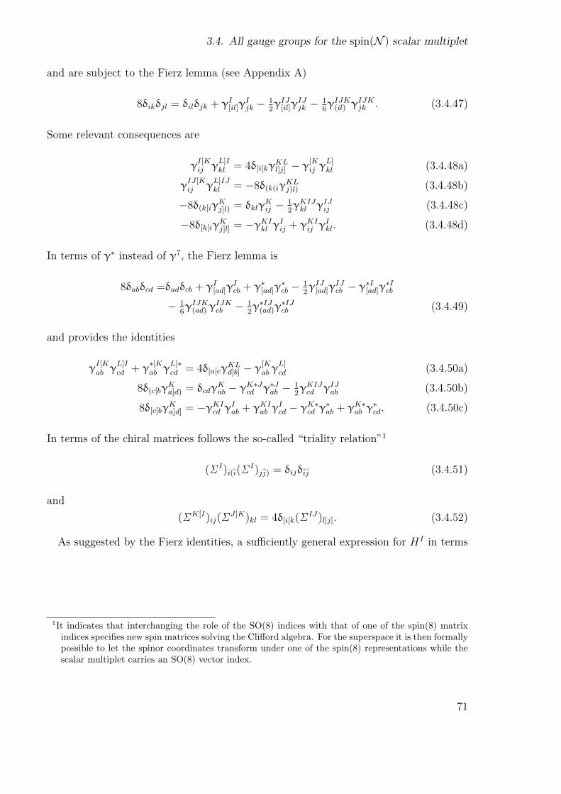
3.4. All gauge groups for the spin(N ) scalar multiplet
and are subject to the Fierz lemma (see Appendix A)
8δikδjl = δilδjk + γI[il]γIjk − 1
2γIJ[il]γ
IJjk − 1
6γIJK(il) γ
IJKjk . (3.4.47)
Some relevant consequences are
γI[Kij γ
L]Ikl = 4δ[i[kγ
KLl]j] − γ
[Kij γ
L]kl (3.4.48a)
γIJ [Kij γ
L]IJkl = −8δ(k(iγ
KLj)l) (3.4.48b)
−8δ(k[iγKj]l) = δklγ
Kij − 1
2γKIJkl γIJij (3.4.48c)
−8δ[k[iγKj]l] = −γKIkl γIij + γKIij γ
Ikl. (3.4.48d)
In terms of γ∗ instead of γ7, the Fierz lemma is
8δabδcd =δadδcb + γI[ad]γIcb + γ∗[ad]γ
∗cb − 1
2γIJ[ad]γ
IJcb − γ∗I[ad]γ
∗Icb
− 16γIJK(ad) γ
IJKcb − 1
2γ∗IJ(ad)γ
∗IJcb (3.4.49)
and provides the identities
γI[Kab γ
L]Icd + γ
∗[Kab γ
L]∗cd = 4δ[a[cγ
KLd]b] − γ
[Kab γ
L]cd (3.4.50a)
8δ(c[bγKa]d) = δcdγ
Kab − γK∗Jcd γ∗Jab − 1
2γKIJcd γIJab (3.4.50b)
8δ[c[bγKa]d] = −γKIcd γIab + γKIab γ
Icd − γK∗cd γ∗ab + γK∗ab γ
∗cd. (3.4.50c)
In terms of the chiral matrices follows the so-called “triality relation”1
(Σ I)i(i(Σ I)jj) = δijδij (3.4.51)
and
(ΣK[I)ij(Σ J ]K)kl = 4δ[i[k(Σ IJ)l]j]. (3.4.52)
As suggested by the Fierz identities, a sufficiently general expression for HI in terms
1It indicates that interchanging the role of the SO(8) indices with that of one of the spin(8) matrixindices specifies new spin matrices solving the Clifford algebra. For the superspace it is then formallypossible to let the spinor coordinates transform under one of the spin(8) representations while thescalar multiplet carries an SO(8) vector index.
71

3. Coupled scalar matter
of an N = 7 spinor is
HIi =γIij
[Aqj qkqk+Bqkqjqk+ Cqkqkqj
]+ γIkl
[Dqkqlqi+ Eqkqiql+ Fqiqkql
]+ γIKkl γ
Kij
[Gqkqlqj+Hqj qkql
]. (3.4.53)
Without loss of generality one can choose H = 0. In order to produce only field-strength
terms, the necessary relations are G = −D, E = 0 and A = −B = −G, leading to
(γ[JHI])m =G(qγIJ q)qm + qm(qγIJq)− γIJkj qkqmqj. (3.4.54)
The third term in this expression can only be converted into a field-strength term if the
gauge group is real SU(2)× SU(2) [21], where
q vv = εvwq w
w εwv. (3.4.55)
In this case, the relation
q[kq|i|qm] = −12q[kqm]qi − 1
2qiq[kqm], (3.4.56)
following from
qltr(qkqm) = qkqmql + qmqkql = qlqkqm + qlqmqk, (3.4.57)
applies and leads to
(γ[JHI])k =32Gc3
[(qγIJ q)qk + qk(qγ
IJq)]. (3.4.58)
With Gc3 = −23a, the resulting solution is
HIi =2
3a[(γIq)iq
kqk − qk(γI q)iqk + (qγI q)qi − (qγIK q)(γKq)i]. (3.4.59)
For fundamental representations one finds no solution.
The analysis in terms of an N = 6 Clifford spinor leads to the same conclusion as for
the N = 7 spinor, with the condition
qa.
=
(Qi
Qi
), (3.4.60)
72
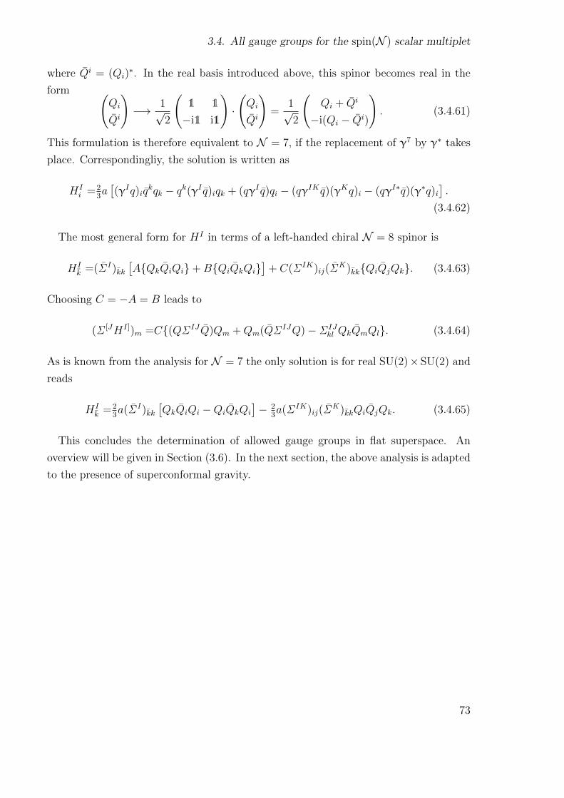
3.4. All gauge groups for the spin(N ) scalar multiplet
where Qi = (Qi)∗. In the real basis introduced above, this spinor becomes real in the
form (Qi
Qi
)−→ 1√
2
(1 1
−i1 i1
)·
(Qi
Qi
)=
1√2
(Qi + Qi
−i(Qi − Qi)
). (3.4.61)
This formulation is therefore equivalent to N = 7, if the replacement of γ7 by γ∗ takes
place. Correspondingliy, the solution is written as
HIi =2
3a[(γIq)iq
kqk − qk(γI q)iqk + (qγI q)qi − (qγIK q)(γKq)i − (qγI∗q)(γ∗q)i].
(3.4.62)
The most general form for HI in terms of a left-handed chiral N = 8 spinor is
HIk =(Σ I )kk
[AQkQiQi+BQiQkQi
]+ C(Σ IK)ij(ΣK )kkQiQjQk. (3.4.63)
Choosing C = −A = B leads to
(Σ [JHI])m =C(QΣ IJQ)Qm +Qm(QΣ IJQ)− Σ IJkl QkQmQl. (3.4.64)
As is known from the analysis for N = 7 the only solution is for real SU(2)×SU(2) and
reads
HIk =2
3a(Σ I )kk
[QkQiQi −QiQkQi
]− 2
3a(Σ IK)ij(ΣK )kkQiQjQk. (3.4.65)
This concludes the determination of allowed gauge groups in flat superspace. An
overview will be given in Section (3.6). In the next section, the above analysis is adapted
to the presence of superconformal gravity.
73

3. Coupled scalar matter
3.5. All gauge groups for the gravitationally coupled
spin(N ) scalar multiplet
The coupling of the spin(N ) scalar multiplet to both a gauge sector and supergravity
demands a solution to the equation
γ[JHI] = F IJq + qGIJ + 14(W IJKLγKL + 4KγIJ)q. (3.5.1)
As mentioned in Section (3.1), this solution is not always given by
HI = HIsg +HI
cs (3.5.2)
or can in some cases be more general. In the following, each case N with matter fields
transforming under irreducible chiral representations of spin(N ) is considered separately.
The on-shell super-Cotton tensor is specified in terms of its corresponding matter current
implied by the coupling to a gauge-coupled scalar and the implications of the coupling
condition are analysed.
3.5.1. N = 4
On shell, the super-Cotton tensor W IJKL ≡ WεIJKL is, in terms of a gauge-coupled
scalar, given by
W = λ16|QiQi|, (3.5.3)
where |.| indicates the trace over gauge-group indices. The complete solution to the
coupling condition is then
HI = HIsg +HI
cs, (3.5.4)
where
HIsg = 1
2( λ
16|QiQi| − 2K)Σ IQ (3.5.5)
and HIcs is the contribution from the gauge sector of the desired gauge group. There is
no other solution both representing the supergravity sector and generalising the gauge
groups possible in flat superspace than the above sum.
74
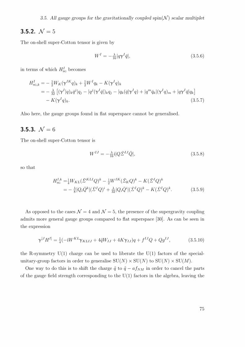
3.5. All gauge groups for the gravitationally coupled spin(N ) scalar multiplet
3.5.2. N = 5
The on-shell super-Cotton tensor is given by
W I = − λ16|qγI q|, (3.5.6)
in terms of which HIsg becomes
HIsg,k =− 1
2WK(γIKq)k + 1
2W Iqk −K(γIq)k
=− λ32
[(γI |q)kqj|qj − |qj(γI q|)kqj − |qk(q|γIq) + |qmqk|(γIq)m + |qγI q|qk
]−K(γIq)k. (3.5.7)
Also here, the gauge groups found in flat superspace cannot be generalised.
3.5.3. N = 6
The on-shell super-Cotton tensor is
W IJ = − λ16
i|QΣ IJQ|, (3.5.8)
so that
HI,ksg = i
4WKL(ΣKLIQ)k − i
2W IK(ΣKQ)k −K(Σ IQ)k
=− λ8|QiQ
k|(Σ IQ)i + λ32|QiQ
i|(Σ IQ)k −K(Σ IQ)k. (3.5.9)
As opposed to the cases N = 4 and N = 5, the presence of the supergravity coupling
admits more general gauge groups compared to flat superspace [30]. As can be seen in
the expression
γ[JHI] = 14(−iWKLγKLIJ + 4qWIJ + 4KγIJ)q + f IJQ+QgIJ , (3.5.10)
the R-symmetry U(1) charge can be used to liberate the U(1) factors of the special-
unitary-group factors in order to generalise SU(N)× SU(N) to SU(N)× SU(M).
One way to do this is to shift the charge q to q − afNM in order to cancel the parts
of the gauge field strength corresponding to the U(1) factors in the algebra, leaving the
75

3. Coupled scalar matter
algebra and the solution HI formally invariant, i.e.
HI =− λ8|QiQ
k|(Σ IQ)i + λ32|QiQ
i|(Σ IQ)k −K(Σ IQ)k
− 2a(Σ I)ijQiQkQj − a(Σ I)kl(QlQ
iQi −QiQiQl). (3.5.11)
This bifundamental representation corresponds to matter in the fundamental represen-
tation of SU(M)×U(1) with arbitrary U(1) charge if the replacement aN→ q2
M+a takes
place. The solution can be written as
HI =− λ8Qβi Q
kβ(Σ IQα)i + λ
32Qβi Q
iβ(Σ IQα)k −K(Σ IQα)k
− 2a(Σ I)ijQαi Q
kβQ
βj − a(Σ I)kl(Qα
l QiβQ
βi −Qα
i QiβQ
βl ). (3.5.12)
Another possibility is to formally gauge U(N)× U(M) and then shift q → q + afNM
in order to produce field-strength terms in the algebra completing the U(N)×U(M) to
SU(N)× SU(M). In this case, it is required that q+ afNM = − i2, thus fixing the gauge
coupling for given q, N and M .
3.5.4. N = 7
The super-Cotton tensor is W IJKL = 16εIJKLSPQWSPQ and
γ[JHI]sg = 1
4
(i3WSPQγ
IJSPQ + 4KγIJ)q. (3.5.13)
As mentioned in Section (3.1) and opposed to the cases N = 4, N = 5 and N = 6, HIsg
cannot be expressed in terms of W IJK , since the general ansatz
HIsg = XWKLMγ
IKLMq + YW IKLγKLq −KγIq (3.5.14)
admits no adequate choice of X, Y .
In terms of a matter current, the on-shell super-Cotton tensor is
W IJK = i λ16|qγIJK q|, (3.5.15)
76
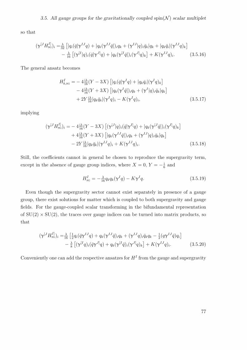
3.5. All gauge groups for the gravitationally coupled spin(N ) scalar multiplet
so that
(γ[JHI]sg)i = λ
32
[|qi(q|γIJq) + |qk(γIJ q|)iqk + (γIJ |q)iqk|qk + |qkqi|(γIJq)k
]− λ
16
[(γ[I |q)i(q|γJ ]q) + |qk(γ[I q|)i(γJ ]q)k
]+K(γIJq)i. (3.5.16)
The general ansatz becomes
HIk,sg =− 4 iλ
16(Y − 3X)
[|qi(q|γIq) + |qkqi|(γIq)k
]− 4 iλ
16(Y + 3X)
[|qk(γI q|)iqk + (γI |q)iqk|qk
]+ 2Y iλ
16|qkqk|(γIq)i −K(γIq)i, (3.5.17)
implying
(γ[JHI]sg)i =− 4 iλ
16(Y − 3X)
[(γ[J |q)i(q|γI]q) + |qk(γ[J q|)i(γI]q)k
]+ 4 iλ
16(Y + 3X)
[|qk(γIJ q|)iqk + (γIJ |q)iqk|qk
]− 2Y iλ
16|qkqk|(γIJq)i +K(γIJq)i. (3.5.18)
Still, the coefficients cannot in general be chosen to reproduce the supergravity term,
except in the absence of gauge group indices, where X = 0, Y = − i6
and
HIsg = − λ
16qkqk(γ
Iq)−KγIq. (3.5.19)
Even though the supergravity sector cannot exist separately in presence of a gauge
group, there exist solutions for matter which is coupled to both supergravity and gauge
fields. For the gauge-coupled scalar transforming in the bifundamental representation
of SU(2)× SU(2), the traces over gauge indices can be turned into matrix products, so
that
(γ[JHI]sg)i = λ
16
[12qi(qγ
IJq) + qk(γIJ q)iqk + (γIJq)iqkqk − 1
2(qγIJ q)qi
]− λ
8
[(γ[Iq)i(qγ
J ]q) + qk(γ[I q)i(γ
J ]q)k]
+K(γIJq)i. (3.5.20)
Conveniently one can add the respective ansatzes for HI from the gauge and supergravity
77
3. Coupled scalar matter
sectors, i.e.
HIi,sg =− 8 iλ
16(Y − 3X)
[qi(qγ
Iq) + qkqi(γIq)k
]− 8 iλ
16(Y + 3X)
[qk(γ
I q)iqk + (γIq)iqkqk]
+ 4Y iλ16qkqk(γ
Iq)i −K(γIq)i (3.5.21)
and
HIi,cs =γIij
[Aqj qkqk+Bqkqjqk+ Cqkqkqj
]+ γIkl
[Dqkqlqi+ Eqkqiql+ Fqiqkql
]+ γIKkl γ
Kij
[Gqkqlqj+Hqj qkql
], (3.5.22)
and solve
(γ[JHI])i =− 8 iλ16
(Y − 3X)[(γ[Jq)i(qγ
I]q) + qk(γ[J q)i(γ
I]q)k]
+ 8 iλ16
(Y + 3X)[qk(γ
IJ q)iqk + (γIJq)iqkqk]− 4Y iλ
16qkqk(γ
IJq)i
− [A(γIJq)iqkqk +Bqk(γIJ q)iqk + Cqkqk(γ
IJq)i]
+ γ[Jijγ
I]kl[Dqkqlqj + Eqkqjql + Fqj qkql]
+ (γIJkl δij − 4δ[k[iγIJj]l] + γ
[Jijγ
I]kl)[Gqkqlqj +Hqj qkql]
+K(γIJq)i.
One can choose the coefficients H = E = F = 0 and G = −A = B = −D such that
(γ[JHI])i =− 8 iλ16
(Y − 3X)[(γ[Jq)i(qγ
I]q) + qk(γ[J q)i(γ
I]q)k]
+ 8 iλ16
(Y + 3X)[qk(γ
IJ q)iqk + (γIJq)iqkqk]− 4Y iλ
16qkqk(γ
IJq)i
− Cqkqk(γIJq)i+ 3
2G(γIJkl δij + δkiγ
IJlj )qkqlqj
+K(γIJq)i.
The couplings are then related by 32G = −a − λ
32= −b + λ
32, since the field-strength
terms of the gauge sector also have to contribute to the supergravity sector. Fixing the
78

3.5. All gauge groups for the gravitationally coupled spin(N ) scalar multiplet
remaining constants X = −Y = − i16
and C = λ64
leads to the solution
HIi =λ
8
[qi(qγ
Iq) + qkqi(γIq)k
]− λ
16
[qk(γ
I q)iqk + (γIq)iqkqk]− λ
64qkqk(γ
Iq)i −K(γIq)i
+ 23(−a− λ
32)[−(γIq)iqkqk + qk(γ
I q)iqk − (qγI q)qi + (qγIK q)(γKq)i]
+ λ64qkqk(γ
Iq)i,
(3.5.23)
which can be rewritten in terms of traces as
HIi =λ
8|qi(q|γIq)− λ
16|qk(γI q|)qk −K(γIq)i
+ 23(−a− λ
32)[−(γIq)i|qkqk|+ |qk(γI q|)iqk − (qγI q)qi + (qγIK q)(γKq)i
].
(3.5.24)
Other gauge groups with a bifundamental representation are not possible.
Regarding fundamental representations, one case derived from the bifundamental rep-
resentation is SU(2) with one of the couplings a, b set to zero. As opposed to the previous
cases, there are more solutions which are not special cases of bifundamental represen-
tations. The supergravity sector in terms of scalars transforming under a fundamental
representation,
(γ[JHI]sg)αi = λ
32
[qβi (qβγ
IJqα) + qβk (γIJ qβ)iqαk + (γIJqβ)iq
kβq
αk + qβk qβ,i(γ
IJqα)k
]− λ
16
[(γ[Iqβ)i(qβγ
J ]qα) + qβk (γ[I qβ)i(γJ ]qα)k
]+K(γIJqα)i, (3.5.25)
has to be compared to the ansatz (choosing H = E = F = 0 and G = −A = B = −D)
(γ[JHI])αi =− 4 iλ16
(Y − 3X)[(γ[Jqβ)i(qβγ
I]qα) + qβk (γ[J qβ)i(γI]qα)k
]+ 4 iλ
16(Y + 3X)
[qβk (γIJ qβ)iq
αk + (γIJqβ)iq
kβq
αk
]− 2Y iλ
16qβk q
kβ(γIJqα)i +K(γIJqα)i
− C1qβk q
kβ(γIJqα)i
+G3(γIJkl δij − δkiγIJjl + δliγIJjk )qαk q
lβq
βj
+G4(γIJkl δij − δkiγIJjl + δliγIJjk )Cαβγδqβk q
lγqδj .
As before, X = −Y = − i16
, and C1 = λ128
cancels the superfluous term in the super-
gravity ansatz. G3 provides both the missing terms in the supergravity ansatz and the
gauge field strength. A solution is then possible for SU(N)×U(1) with the specification
79

3. Coupled scalar matter
G3 = λ32
= a− λ32
= aN− q2
Nand is given by
HIi = λ
16
[qβi (qβγ
Iqα) + qβk qβ,i(γIqα)k
]− λ
32
[qβk (γI qβ)iq
αk + (γIqβ)iq
kβq
αk
]−K(γIq)i
− λ32
(γIqα)iqkβq
βk + λ
32qαk (γI qβ)iq
βk − λ
32(qαγI qβ)qβi + λ
32(qαγIK qβ)(γKqβ)i. (3.5.26)
For SO(N), the ansatz for HIcs cannot provide field-strength terms; however, the
missing terms in the supergravity ansatz can be explained by an SO(N) field strength
cancelling them. Concretely, in the supergravity sector in terms of a scalar transforming
under SO(N),
(γ[JHI]sg)i = λ
32
[2(q[βγ
IJqα])qi,β + 2(γIJqβ)iqkβq
kα
]− λ
162(γ[Iqβ)i(qβγ
J ]qα) +K(γIJqα)i,
(3.5.27)
the first term can be cancelled by choosing a = − λ32
. The solution depends therefore
only on λ and is given by
HIα =λ
8qβ(qβγ
Iqα)− λ16
(γIqβ)qkβqkα −KγIqα. (3.5.28)
This SO(N) gauge group can further be promoted to spin(7) by taking 3G4 = −32λ32
.
The corresponding solution reads
HIα =λ
8qβ(qβγ
Iqα)− λ16
(γIqβ)qkβqkα − λ
64Cαβγδ[(q
βγIKqγ)(γKqδ)− (qβγIqγ)qδ]−KγIqα.(3.5.29)
3.5.5. N = 8
The super-Cotton tensor is self-dual and
Σ [JHI]sg = 1
4(W IJKLΣKLQ+ 4KΣ IJQ). (3.5.30)
The ansatz
HIsg = XW IKLM ΣKLMQ+ 2KΣ IQ (3.5.31)
provides no solution off shell since
Σ [JHI]sg = XW [I|KLM |Σ J ]KLMQ+ 3XW IJLMΣLMQ− 2KΣ IJQ. (3.5.32)
80

3.5. All gauge groups for the gravitationally coupled spin(N ) scalar multiplet
The on-shell super-Cotton tensor is
W IJKL = λ16|QΣ IJKLQ|, (3.5.33)
so that
Σ [JHI]sg = λ
32|QiQi|(Σ IJQ)− λ
16|Qi(Σ IJQ|)Qi − λ
16(Σ IJ |Q)Qi|Qi
− λ16|Q(Q|Σ IJQ)− λ
16|QiQ|(Σ IJQ)i +KΣ IJQ. (3.5.34)
The ansatz becomes
HIsg =X λ
16
[24|Qi(Σ I Q|)Qi + 24(Σ I |Q)Qi|Qi − 6|QiQi|(Σ IQ)
]−KΣ IQ, (3.5.35)
implying
Σ [JHI]sg =−X λ
16
[24|Qi(Σ IJQ|)Qi + 24(Σ IJ |Q)Qi|Qi − 6|QiQi|(Σ IJQ)
]+KΣ IJQ. (3.5.36)
Similarly to the case N = 7, the coefficients cannot in general be chosen to reproduce
the supergravity term, except in the absence of gauge-group indices, where X = 128
and
HIsg = 3
2λ16Q2Σ IQ−KΣ IQ. (3.5.37)
However, a solution with a gauge-coupled scalar field exists for the combined gauge
and supergravity sector. Conveniently, the on-shell ansatz of the gauge sector to the one
for the supergravity sector can be added. For a bifundamental representation, the only
possibility remains real SU(2)× SU(2) [21]. In this case, it can be written
Σ [JHI]sg =− λ
8Qi(Σ IJQ)Qi − λ
16(Σ IJQ)QiQi
− λ16Q(QΣ IJQ) + λ
16(QΣ IJQ)Q+KΣ IJQ (3.5.38)
and for the combined ansatz
Σ [JHI] =−X λ16
[48Qi(Σ IJQ)Qi + 36(Σ IJQ)QiQi
]+KΣ IJQ
−[A(Σ IJQ)QiQi +BQi(Σ IJQ)Qi
]+ C
[32(QΣ IJQ)Q+ 3
2Q(QΣ IJQ) +Qi(Σ IJQ)Qi − (Σ IJQ)QiQi
]. (3.5.39)
81

3. Coupled scalar matter
The couplings must fulfil a + b = −3C and a − b = λ8
[21], while e.g. X = 124
, C = B
and A = −C − λ32
. The solution is
HI = λ16
[2Qi(Σ I Q)Qi + 3
2(Σ IQ)QiQi
]−KΣ IQ
+ 13(2a− λ
8)[(Σ IQ)QiQi −Qi(Σ I Q)Qi − (QΣ IKQ)(ΣKQ)]
− λ32
(Σ IQ)QiQi. (3.5.40)
As for gauge groups with fundamental representations, one example is given by SU(2),
realised by setting a or b to zero in the above gauging of SU(2)× SU(2). In general, the
supergravity sector in terms of scalars transforming under a fundamental representation
reads
Σ [JHI]sg = λ
32Qβi Q
iβ(Σ IJQα)− λ
16Qβi (Σ IJQβ)Qα
i − λ16
(Σ IJQβ)QiβQ
αi
− λ16Qβ(QβΣ IJQα)− λ
16Qβi Qβ(Σ IJQα)i +KΣ IJQα. (3.5.41)
Comparing with the combined ansatz
Σ [JHI] =−X λ16
[24Qβ
i (Σ IJQβ)Qαi + 24(Σ IJQβ)Qi
βQαi − 6Qβ
i Qiβ(Σ IJQα)
]+KΣ IJQα
−[A(Σ IJQ)QiQi +BQi(Σ IJQ)Qi
]+ C3[(QαΣ IJQβ)Qβ +Qα(QβΣ IJQβ)−Qα
i Qk,β(Σ IJQβ)i
+Qαi (Σ IJQβ)Qβ
i − (Σ IJQα)Qi,βQβi ], (3.5.42)
a solution exists for SU(N)× U(1) with a = −λ8
and q2 = −λ8( 1N− 1
2), reading
HI,α = λ32
[Qβi Q
iβ(Σ IQα) + 2Qα
i Qiβ(Σ IQα)]− λ
16(QαΣ IKQβ)(ΣKQβ)
+ 2KΣ IQα. (3.5.43)
For a scalar transforming under SO(N), the supergravity sector becomes
Σ [JHI]sg =− λ
8Qβ(QβΣ IJQα) + λ
32QβiQ
iβ(Σ IJQα)− λ
8(Σ IJQβ)Qi
βQαi
+KΣ IJQα. (3.5.44)
If the SO(N) coupling is chosen to be a = λ16
[21], the first term is cancelled and a
82

3.5. All gauge groups for the gravitationally coupled spin(N ) scalar multiplet
solution can be given as
HI = λ32
[4(Σ IQβ)Qi
βQαi −Q
βiQ
iβ(Σ IQα)
]−KΣ IQα. (3.5.45)
This solution can be modified for spin(7) to
HI = λ32
[4(Σ IQβ)Qi
βQαi −Q
βiQ
iβ(Σ IQα)
]+ λ
32Cαβγδ(Q
βΣ IKQγ)(ΣKQδ)−KΣ IQα.
(3.5.46)
This concludes the determination of allowed gauge groups in curved superspace, where
the scalar multiplet is additionally coupled to superconformal gravity. An overview of
the results from the last two sections is given in the next section.
83

3. Coupled scalar matter
3.6. Overview of gauge groups
The following table summarises the findings from the previous two sections. The columns
“fundamental” and “bifundamental” list the allowed gauge groups for which the scalar
fields are in the fundamental or bifundamental representation, respectively. Together
with the values N it is implied that the scalar multiplet transforms under an irreducible
(chiral) representation of spin(N ). The lines denoted by “+SG” contain the allowed
gauge groups in curved superspace, i.e. in the presence of conformal supergravity. For
N = 4 and N = 5 they are the same as in flat space. The subscripts of the group factors
indicate the relative coupling constants.
fundamental bifundamental
N = 4 SU(N)a × U(1)a−a/N U(M)a × U(N)−a
Sp(N)a × U(1)−a SU(M)a × SU(N)−a × U(1)a/N−a/M
Sp(M)a × SO(N)−a
spin(7)a × SU(2)−a
N = 5 SU(N)a × U(1)a−a/N U(M)a × U(N)−a
Sp(N)a × U(1)−a SU(M)a × SU(N)−a × U(1)a/N−a/M
Sp(M)a × SO(N)−a
spin(7)a × SU(2)−a
N = 6 SU(N)a × U(1)a−a/N U(M)a × U(N)a
Sp(N)a × U(1)−a SU(M)a × SU(N)a × U(1)a/N−a/M
Sp(M)a × SO(2)a
+SG SU(N)× U(1) SU(M)a × SU(N)a
N = 7 SU(2)a × SU(2)a
+SG SU(N)−λ/8 × U(1)(2−N)λ/16 SU(2)a × SU(2)a−λ/8
SO(N)−λ/16
spin(7)−λ/16
N = 8 SU(2)a × SU(2)a
+SG SU(N)−λ/4 × U(1)(2−N)λ/8 SU(2)a × SU(2)a−λ/4
SO(N)−λ/8
spin(7)−λ/8
84

3.6. Overview of gauge groups
As mentioned during the above analysis, the groups with fundamental representation
in flat space are equivalent to corresponding groups with bifundamental representation
for a certain case of N,M . The same is true in curved superspace, except for SO(N)
and spin(7) in the cases N = 7, 8.
It is worth to note that for the cases N = 6, 7, 8 the coupling constants of the two
group factors with bifundamental representation appear with equal sign, which is due
to the conventional ordering of the conjugated scalar fields in the on-shell expressions
for the left- and right-acting field strengths, as defined in Section (3.4). This however
correspond to opposite signs of the matter currents, which contain the conjugate fields
in the usual order. Concretely, since for N = 6, 7, 8 the matrices γIJ have the property
QγIJQ =− QγIJQ (3.6.1a)
QΣ IJQ =− QΣ IJQ, (3.6.1b)
the sign of the right-acting field strength gets reverted in the usual ordering.
This sign difference is reflected in opposite signs of the two Chern-Simons terms for
the two group factors. It is essential for describing the world-volume theory of M2-
branes. Since one Chern-Simons term is parity-odd due to the cubic vector fields, the
interchange of left- and right-acting gauge fields under parity can be imposed in order
to leave the combined Chern-Simons terms invariant [10]. The requirement of parity
invariance comes from the principle that M2-branes correspond to the strong-coupling
limit of D2-branes, which are parity-even.
The results in the table have been partially present in various places in the literature.
Regarding flat space, the groups for N = 4, except for spin(7)a × SU(2)−a, had been
initially discovered in [13], and extended for N = 5 in [15]. Classifications for N = 6
were given in [14], [12] and [16]. The unique gauge group for N = 8 appeared in the
BLG model [9, 8] and subsequent comments, e.g. [10]. The group spin(7)a × SU(2)−a
was found in [17], where also the case N = 7 had been mentioned. As for the presence
of supergravity, the group SO(N) for N = 8 was found in [21] and the generalisation
to SU(M) × SU(N) of N = 6 was mentioned in [30]. The groups with fundamental
representation SU(N)×U(1) and spin(7) for N = 7, 8 [32] are new results of the present
analysis.
85


4. Topologically massive supergravity
In this chapter, the gravitationally coupled spin(N ) scalar multiplet is interpreted as a
conformal compensator in order to realise extended topologically massive supergravities
and to specify the corresponding values of µ`.
In Section (4.1), basic properties of three-dimensional Einstein-Hilbert gravity with a
negative cosmological constant, conformal gravity, and topologically massive gravity are
reviewed.
In Section (4.2), the relation between the cosmological constant of anti-de Sitter space
and the geometry of anti-de Sitter superspace is established. Further, the action for the
scalar conformal compensator is given.
In Section (4.3), the spin(N ) superfield describing the compensator multiplet is intro-
duced into anti-de Sitter superspace. Consistency with this background together with
previous results directly leads to a formula for µ` in the cases 4 ≤ N ≤ 8, which is eval-
uated. Subsequently, it is analysed how the values of µ` can change if the compensator
transforms under additional gauge groups.
4.1. Einstein gravity and topologically massive gravity
In three space-time dimensions, the Riemann tensor R[mn][kl] = R[kl][mn] is dual to a
symmetric tensor of rank two
Rmnkl ≡ εmnrεklsRrs. (4.1.1)
It is completely determined by the Ricci tensor and curvature scalar, since
Rmn = Rmn + Rgmn = Rmn − 12Rgmn, (4.1.2a)
which translates back to
Rrsmn = 4R[m[rgs]n] −Rgm[rgs]n. (4.1.3)
87

4. Topologically massive supergravity
In consequence, the Einstein equation with negative cosmological constant Λ = −`−2
0 = Rmn − 12gmnR− gmn
1
`2(4.1.4)
completely fixes the geometry to describe space-time with constant negative curvature,
or anti-de Sitter space, specified by
R = − 6
`2(4.1.5a)
Rmn = −2gmn1
`2. (4.1.5b)
This leaves no freedom for a locally propagating graviton. However, the solution of the
Einstein equation with negative cosmological constant can be generalised to a metric
which describes the analogue of a black hole in four dimensions, known as the BTZ
black hole [23]. Its parameter corresponding to the mass is positive when describing a
black hole and can take a separated negative value to recover the anti-de Sitter metric.
Asymptotically, the BTZ metric always becomes the anti-de Sitter metric. Gravity on
this asymptotic anti-de Sitter space can be described by a two dimensional conformal
field theory on its boundary [24] with the total central charge
cR + cL =3`
2G. (4.1.6)
The left- and right-moving modes correspond to massless gravitons propagating on this
boundary.
The model of cosmological topologically massive gravity is given by the action [25]
S =1
κ2
∫d3x e
(R + 2`−2
)+
1
4µκ2
∫d3x e εmnl
(ωabmRnl,ab − 2
3ωabmω
cn,b ωl,ca
), (4.1.7)
where κ2 = 16πG. It is the sum of the Einstein-Hilbert action and the conformal gravity
action for the spin connection ωm(e). The resulting equations of motion are
Gmn + 1µCmn = 0 (4.1.8)
88

4.1. Einstein gravity and topologically massive gravity
with
Gmn =Rmn − 12gmnR− gmn
1
`2(4.1.9a)
Cmn =ε klm ∇k(Rln − 1
4glnR). (4.1.9b)
Vanishing of the Cotton tensor Cmn is equivalent to a conformally flat space-time. There-
fore, conformal gravity alone also has no propagating degrees of freedom. While the anti-
de Sitter solution for pure cosmological Einstein-Hilbert gravity, including black holes
and massless boundary gravitons, is still valid, the presence of the conformal-gravity
term gives rise to a massive propagating graviton with mass µ. In absence of the cosmo-
logical constant, the Einstein-Hilbert term is usually taken with the sign opposite to the
one above, in order to ensure a positive energy for the graviton. This, however, would
cause the mass of the BTZ black hole to become negative [40].
The central charges of the boundary conformal field theory are modified due to the
conformal-gravity term, becoming [27]
cR =3`
2G(1 + 1
µ`) (4.1.10a)
cL =3`
2G(1− 1
µ`). (4.1.10b)
Choosing the appropriate sign for positive-mass black holes, the analysis of the gravi-
ton modes in presence of the negative cosmological constant [26] then shows that for
general values of µ` the theory suffers from negative energies of the gravitons. Only
in the special case µ` = 1, the massive and left-moving gravitons become degenerate
and non-propagating, leaving a chiral conformal field theory with (cR, cL) = (3`/G, 0)
[26, 41] and a right-moving degree of freedom with positive energy. This model is called
chiral gravity or topologically massive gravity at the chiral point.
The parameter µ` can freely be chosen to have this most sensible value of µ` =
1. However, in the following it will be shown that µ` is fixed by the superconformal
geometry for N ≥ 4 supersymmetric topologically massive gravity, where the Einstein-
Hilbert action is realised via a superconformal compensator [31, 32]. The resulting
topologically massive gravities and values of µ` will be classified corresponding to all
possible gauged compensators.
89
4. Topologically massive supergravity
4.2. Conformal supergravity and conformal
compensators
In the supersymmetric case, the Chern-Simons action for conformal gravity is replaced
by the action for extended superconformal gravity [39]. Most importantly, besides the
terms for fermionic and auxiliary fields, it is supplemented by a Chern-Simons term for
the gauge field BIJm of the SO(N ) local structure group
1
4µκ2
∫d3x e εmnl
(−2BIJ
m Fnl,IJ − 43BIJm B
JKn BKI
l
). (4.2.1)
In view of the anti-de Sitter solution of cosmological Einstein gravity, the geometries
of anti-de Sitter space and the anti-de Sitter background of superconformal gravity can
be compared using the algebra of covariant derivatives. The Riemann tensor is defined
by the commutator
[∇m,∇n]V k =(
2∂[mΓkn]l + 2Γk[m|p|Γpn]l
)V l ≡ R k
mn lVl = − 2
`2δk[mgn]lV
l, (4.2.2)
which can be translated to the tangent space as
[∇a,∇b]Vc = − 2
`2δc[aηb]dV
d. (4.2.3)
Comparison with the commutator from superconformal geometry in the background of
anti-de Sitter superspace [38]
[Da,Db]Vc = −4K2MabV
c = −8K2δc[aηb]dVd (4.2.4)
shows that the cosmological constant is generated by the value of the field K with [31]
`−1 = 2|K|. (4.2.5)
The Einstein-Hilbert term can be realised by a supersymmetric conformal compensator
q subject to the bosonic part of the conformally invariant action [42]
Sbos. =
∫d3x e
(−1
2(Daq)(Daq)− 1
16R|q|2 + λ(|q|2)3
), (4.2.6)
where λ is a constant. The Einstein-Hilbert term is recovered in the super-Weyl gauge
90
4.3. Extended topologically massive supergravity
for q, where
|q|2 = 16κ−2. (4.2.7)
This action is naturally part of the action for the gravitationally coupled spin(N ) scalar
multiplet [29, 21]. It would be desirable to obtain it from the superfield action (3.2.22)
presented in Chapter 3; however, the action would have to be formulated in a locally
scale invariant way, and the relation of the Riemann scalar R in terms of the geometry
of conventional curved superspace to the fields appearing in the component action would
have to be established, possibly accounting for the differential relations appearing in the
expression for the dimension-two Lorentz curvature derived in Chapter 2.
4.3. Extended topologically massive supergravity
4.3.1. Fixation of µ`
In order to agree with the background defining anti-de Sitter superspace, the superfield
describing the spin(N ) scalar compensator multiplet has to be covariantly constant
DAQ = 0. (4.3.1)
In consequence, the anticommutator of spinor covariant derivatives acting on Q
D Iα,D
Jβ Q = 0 (4.3.2)
implies the algebraic condition [31, 32]
4KγIJQ = −W IJKLγKLQ. (4.3.3)
Conveniently, this condition is equivalent to qJ
[α,β] = 0 or HJ = 0 [32]. Using the relations
K =1
2`(4.3.4)
and
W IJKL =µκ2
16|qγIJKLq| (4.3.5)
leads to2
`γIJq = −µκ
2
16|qγIJKLq|γKLq. (4.3.6)
91

4. Topologically massive supergravity
Replacing the gravitational coupling with
κ2 = 16|q|−2 (4.3.7)
and multiplying by γIJ leads to the formula
(µl)−1q = 12N (N−1)
|q|−2|qγIJKLq|γIJKLq. (4.3.8)
Its evaluation yields [32]
N = 4 5 6 7 8
(µ`)−1 = 1 3/5 1 2 3
where for N = 6 the formula was adjusted due to the additional U(1) field strength
associated with the local structure group, contributing to the super-Cotton tensor.
4.3.2. Gauged compensators
For a gauge-coupled compensator, the adapted condition for anti-de Sitter background
HI = HIsg +HI
cs = 0 (4.3.9)
generally leads to deformations of µ, which can involve the gauge coupling, special
properties of the gauge group and the number of compensator components with non-
vanishing values. If the compensator transforms under a bifundamental representation,
the deformation typically vanishes.
Usually, if HIcs can be written in the form
(HIcs)
αa = Xqγc q
cγ(γ
I) ba q
αb (4.3.10)
for some subset of the range of spin(N ) indices a and gauge indices α, then there is a
shift
µ −→ µ+ 32Xκ−2. (4.3.11)
Special effects can appear, if the gauge and supergravity sectors depend on each other.
In the following, features of each case N are commented.
92

4.3. Extended topologically massive supergravity
N = 4 For N = 4 the deformation vanishes for compensators in bifundamental rep-
resentations due to the opposite signs of the coupling constants of the factor groups
and to the antisymmetry of the spin(7) tensor Crsvw. For the groups with fundamental
representation, since one can choose only one gauge component to be non-vanishing, the
deformation likewise cancels.
N = 5 For N = 5, the same statements as for N = 4 hold.
N = 6 For N = 6, the statements made for N = 4 and N = 5 still apply; however,
the gauge group SU(N)× U(1) in the presence of supergravity causes a deformation of
µ. In this case, the AdS background requires
K(Σ IQα)k =− λ8Qβi Q
kβ(Σ IQα)i + λ
32Qβi Q
iβ(Σ IQα)k
− 2a(Σ I)ijQαi Q
kβQ
βj − a(Σ I)kl(Qα
l QiβQ
βi −Qα
i QiβQ
βl ). (4.3.12)
In general, only one component of the matrix Qαi can be non-vanishing, leaving µ` = 1.
However, in the special case where a = λ16
, or
K(Σ IQα)k =− λ32Qβi Q
iβ(Σ IQα)k + λ
16Qαi Q
iβ(Σ IQβ)k, (4.3.13)
one can choose Qiα = 4κ−1p−1δiα, where α = 1, ..., p ≤ 4. This leads to the relation
1
2`= −µκ
2
3216κ−2 +
µκ2
1616κ−2 1
p(4.3.14)
and to the formula [32]
(µ`)−1 =2
p− 1. (4.3.15)
N = 7 For the compensator coupled to supergravity and the gauge group SU(2) ×SU(2), the condition
KγIabqb =λ8|qaqb|γIbcqc − λ
16|qcqb|γIabqc
+ 23(a− λ
32)[−γIabqb|qcqc|+ γIab|qcqb|qc − (qγI q)q + (qγIK q)(γKq)
](4.3.16)
is realised by one non-vanishing spin(7) component, leaving (µ`)−1 = 2. Similarly,
compensators transforming under a possible fundamental representation do not realise
any deformation of (µ`)−1 [32].
93

4. Topologically massive supergravity
N = 8 For the compensator coupled to supergravity and the gauge group SU(2) ×SU(2), the AdS condition yields (µ`)−1 = 3 [21].
The gauge group SO(N) allows a deformation of µ`. The condition is
K(Σ IQα)k = λ32
[4(Σ IQβ)kQi
βQαi −Q
βiQ
iβ(Σ IQα)k
]. (4.3.17)
One can choose Qiα = 4κ−1p−1δiα, where α = 1, ..., p ≤ 8. This leads to
1
2`= −µκ
2
3216κ−2 +
µκ2
816κ−2 1
p(4.3.18)
or [33]
(µ`)−1 =4
p− 1. (4.3.19)
In summary, the gravitationally coupled scalar multiplet was used as a conformal
compensator, which naturally realises topologically massive supergravities with fixed
value of µ` for N ≥ 4. This fixation is mainly owed to the fact that the super-Cotton
tensor appearing for N ≥ 4 contains the SO(N ) field strength whose corresponding
coupling constant involves µ. The relation between µ and the anti-de Sitter radius ` is
implied by the background of anti-de Sitter superspace. Using an ungauged compensator
field, the values µ` are given by a generic formula which can be evaluated for the specific
cases N . For a gauged compensator, a number of gauge components can be given an
expectation value generating the gravitational coupling constant. This has no effect for
N = 4, 5, 7, but leads to specific diversifications for N = 6 with gauge group SU(N)
and N = 8 with gauge group SO(N) given by formulas involving the number of chosen
gauge components.
94
5. Conclusion
In this thesis, the coupling of scalar supermultiplets to superconformal Chern-Simons
gauge theories and superconformal gravity has been described in the framework of N -
extended superspace.
As for the gauge coupling, a list of all possible gauge groups for theories with 4 ≤N ≤ 8 supersymmetries has been produced. It agrees with the classifications found
in various places in the literature. However, the superfield formalism employed here
proves more powerful in several regards: First of all, it does not require any knowledge
about the component actions of the theories, but rather provides the superfield action
principle readily producing such component actions. Furthermore, these actions are
delivered for all N , only requiring the gauge-group-dependent field HI appearing in the
transformation law of the fermionic matter field.
Most importantly for the main goal of this thesis, the superfield analysis is equally
suited for superconformal gravity-coupled matter. The thorough investigation of mod-
ifications or new emergence of gauge groups in curved superspace, as compared to flat
superspace, has produced some new results, completing the existing knowledge in this
regard.
For the topologically massive gravities realised by using the coupled matter field as
a conformal compensator, the resulting fixed values µ` have been determined and its
possible modifications due to the presence of gauge groups have been discussed. These
values are important concerning the stability, or positive energies, of topologically mas-
sive gravity. The value µ` = 1 preferred by the model of chiral gravity is indeed implied
by N = 4 and N = 6 supersymmetry, and can also be achieved for N = 8 with gauge
group SO(N).
However, as was mentioned in the introduction, the conformal compensator generates
the opposite sign of the Einstein-Hilbert action. This corresponds to a negative mass
of the BTZ black hole. This problem has often been noted in the literature [29], with
no satisfying conclusion so far. One promising discussions is given in [43]. There, it is
conjectured that the negative-mass black holes may be excluded from interaction with
95

5. Conclusion
the physical matter fields or, in other words, could never be formed by the collapse of
the positive-energy matter and therefore would live in a different superselection sector
of the theory.
Such a solution would be necessary in view of a positive total mass of topologically
massive gravity. General relativity in four space-time dimensions possesses various
positive-energy theorems, stating that space-times with appropriate asymptotic sym-
metries allowing for conserved asymptotic charges have non-negative mass with unique
zero-energy states. Classic examples are asymptotically-Minkowski and -anti-de Sitter
spaces. The most simple proofs for these theorems can be derived from supergravity
[44], whose positivity of energy is implied by the supersymmetry algebra [45]. Also for
three-dimensional cosmological topologically massive gravity, positive energy has been
established by its embeddability in simple supergravity [46]. The value µ` relevant for
perturbative stability is however free to choose. The feature of the new extended topo-
logically massive supergravities is the fixation of this parameter, in some cases to the
value µ` = 1 required by perturbative stability. As is known to be possible in four di-
mensions [47], it could therefore be beneficial to generalise the analysis of mass-positivity
to these extended supergravities.
96

A. Symmetry groups
A.1. Fundamental representations
If the elements of a Lie group are represented by matrices M , a vector v transforms
under the standard-fundamental representation as
v −→M · v, (A.1.1)
a dual vector transforms under the dual representation as
v(∗) −→ (M−1)T · v(∗), (A.1.2)
a complex conjugate vector transforms under the complex conjugate representation as
v∗ −→M∗ · v∗, (A.1.3)
and a dual complex conjugate vector transforms under the dual complex conjugate
representation as
v∗(∗) −→ (M−1)† · v∗(∗). (A.1.4)
Dual vectors map vectors to numbers according to
v(∗)(w) ≡ (v(∗))T · w ∈ C. (A.1.5)
If there is an isomorphism between a vector w and a dual vector w(∗) via a scalar product
〈w, v〉 = (w(∗))T · v (A.1.6)
(holding for all v) being invariant under the group transformations, the two representa-
tions are equivalent. If the scalar product is described by a metric g
〈w, v〉 = wT · gT · v, (A.1.7)
97

A. Symmetry groups
the metric is a linear map between w and w(∗)
w(∗) = g · w (A.1.8)
If the elements of a group are defined to leave a certain matrix g invariant, i.e.
g−1 ·MT · g = M−1, (A.1.9)
then g is such a metric.
A.2. Index notation
Components of vectors are denoted by a lower index, components of dual vectors are
denoted by an upper index. Same named upper and lower indices are summed over.
The scalar product reads
〈w, v〉 = (w(∗))ivi. (A.2.1)
A metric mapping vectors to dual vectors has two upper indices (for real groups the (∗)superscript is usually omitted)
(w(∗))i = gijwj (A.2.2)
and the inverse metric has two lower indices
wi = (g−1)ij(w(∗))j = (w(∗))j((g−1)T)ji ≡ (w(∗))jgji. (A.2.3)
The indices of the transformation matrices can be deduced and are summarised in the
relation
g ·M · g−1 =(M−1)T (A.2.4a)
gijM kj (g−1)kl =((M−1)T)il. (A.2.4b)
Examples. Elements of the pseudo-orthogonal group SO(M,N) are real and
have g = η, where
η = diag(−1, ..,−1, 1, .., 1), (A.2.5)
and elements of the symplectic group Sp(N) have g = ε where ε is antisymmetric.
98

A.3. Generators
Elements of the unitary group SU(N) fulfil
M † = M−1, (A.2.6)
identifying the dual and complex conjugate representations. The isomorphism between
the fundamental and dual representations is given by complex conjugation and the scalar
product is
〈w, v〉 = (w∗)T · v. (A.2.7)
A.3. Generators
A Lie-group element is given by the exponential
M = eX = eXATA , (A.3.1)
where X is the generator of this group element and is expanded in the basis elements
TA depending on the group, which are the generators of the group. Due to the formula
eX · eY = eX+Y+12
[X,Y ]+112
[X[X,Y ]]+... (A.3.2)
the generators must fulfil a Lie algebra
[TA, TB] = fCABTC (A.3.3)
where fCAB are constants.
For the fundamental representation of the special unitary group acting on vectors
with components xi, the matrix X ji is anti-hermitian,
X∗ = −X. (A.3.4)
It is expanded in a basis TA
X ji = XA(TA) ji (A.3.5)
with the normalisation
tr(TA, TB) = δAB. (A.3.6)
99
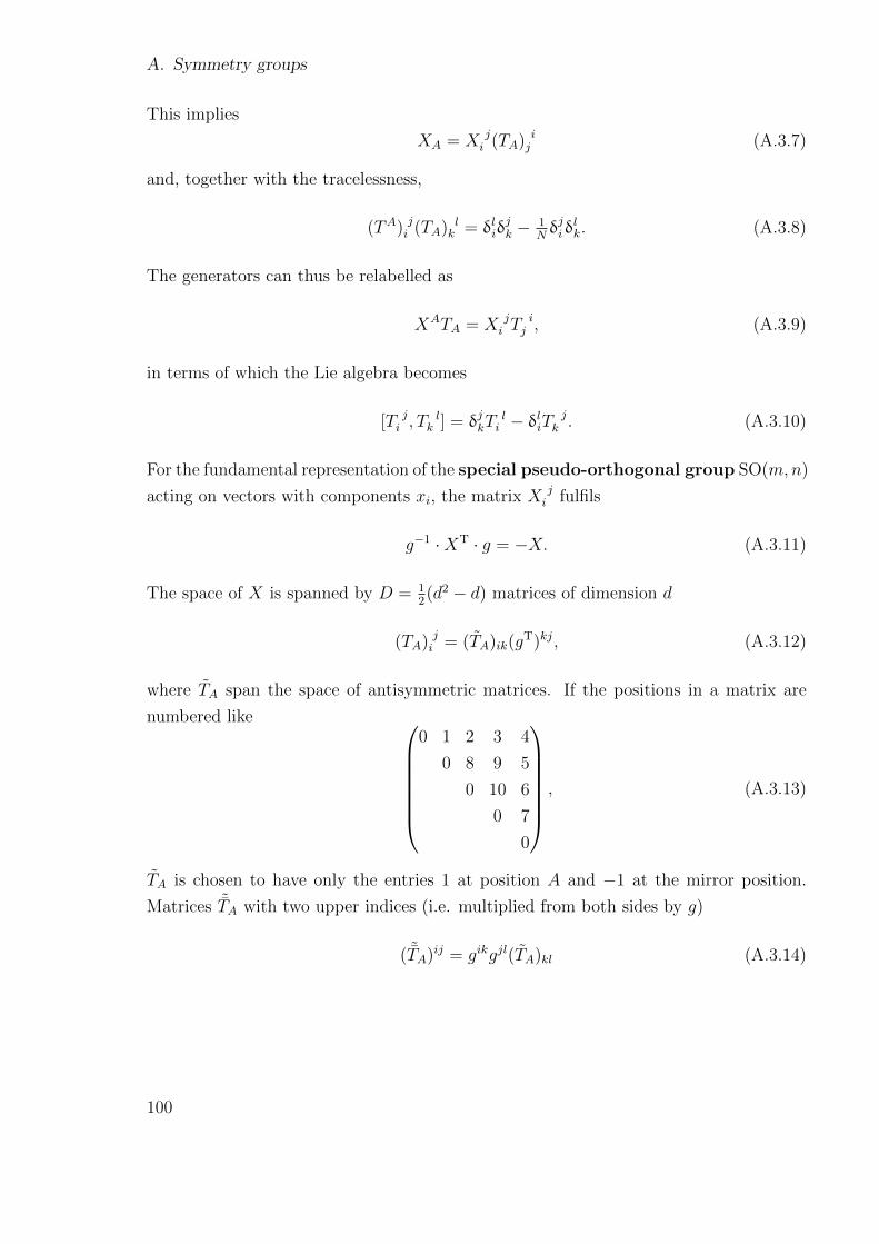
A. Symmetry groups
This implies
XA = X ji (TA) i
j (A.3.7)
and, together with the tracelessness,
(TA) ji (TA) lk = δliδ
jk − 1
Nδjiδ
lk. (A.3.8)
The generators can thus be relabelled as
XATA = X ji T
ij , (A.3.9)
in terms of which the Lie algebra becomes
[T ji , T
lk ] = δjkT
li − δliT
jk . (A.3.10)
For the fundamental representation of the special pseudo-orthogonal group SO(m,n)
acting on vectors with components xi, the matrix X ji fulfils
g−1 ·XT · g = −X. (A.3.11)
The space of X is spanned by D = 12(d2 − d) matrices of dimension d
(TA) ji = (TA)ik(gT)kj, (A.3.12)
where TA span the space of antisymmetric matrices. If the positions in a matrix are
numbered like 0 1 2 3 4
0 8 9 5
0 10 6
0 7
0
, (A.3.13)
TA is chosen to have only the entries 1 at position A and −1 at the mirror position.
Matrices ˜TA with two upper indices (i.e. multiplied from both sides by g)
( ˜TA)ij = gikgjl(TA)kl (A.3.14)
100

A.4. Spin groups
are related to TA by˜TA =
(−T1, ...,−TS, TS+1, ..., TD
), (A.3.15)
where S = 2mn− n. Therefore,
tr(TA˜TB) = −2ηAB (A.3.16)
where η is the metric of the group SO(T, S), where T = D − S. It follows that
tr(TATB) = −2ηAB, (A.3.17)
because
(TA) ji (TA) ij = (TA)ikg
kj(TA)jlgli = (TA)ik(
˜TA)ki. (A.3.18)
Then
XA = −12X ji (TA) i
j (A.3.19)
and
(TA) ji (TA)kl = (T kl) ji = 2δ[ki g
l]j. (A.3.20)
This suggests the relabelling
XATA = 12X ijTij (A.3.21)
and the Lie algebra becomes
[T ab, T cd] = −4g[c[aT b]d]. (A.3.22)
A.4. Spin groups
The N -dimensional Clifford algebra is
γI ,γJ = 2δIJ . (A.4.1)
The matrices
N IJ = 14[γI ,γJ ] = 1
2γIJ (A.4.2)
101

A. Symmetry groups
solve the SO(N) Lie algebra and are the generators defining the group spin(N). One
solution for the Clifford algebras of dimension N = 2m and N = 2m+ 1 is
γ1 = σ1 ⊗ 1⊗ ...⊗ 1
γ2,...,2m = iσ2 ⊗ iγ1,...,N−1
γ∗ = γ2m+1 ≡ −imγ1 · ... · γ2m = σ3 ⊗ 1⊗ ...⊗ 1, (A.4.3)
where γ solve the N = 2m− 1 dimensional Clifford algebra and each line consists of m
Kronecker-factors of 2 × 2 matrices. For N = 2m, the generators of spin(N) commute
with the matrices
PL/R = 12(1± γ∗), (A.4.4)
which project on the generators of irreducible representations. These are called left- and
right-handed and transform under the generators defined by the chiral Clifford algebra
Σ IΣ J = δIJ + Σ IJ (A.4.5a)
Σ IΣ J = δIJ + Σ IJ , (A.4.5b)
where
γI =
(0 Σ I
Σ I 0
). (A.4.6)
The map to the corresponding SO(N) representation is given by
vI = ψa(γI) ba χb, (A.4.7)
which transforms as an SO(N) vector since for infinitesimal parameters ωIJ ,
(A−1) ac (γI) b
a Adb = (1− 1
4ωKLγKL) a
c (γI) ba (1 + 1
4ωPQγPQ) d
b
= (γI) dc − 1
4ωKL[γKL, γ
I ] dc
= (γI) dc + ωIL(γL) d
c . (A.4.8)
An SO(N) vector is therefore equivalent to a matrix in the space spanned by γI according
to
v ji = vI(γI)
ji ⇐⇒ vI = 1
2m(γI)
ji v
ij . (A.4.9)
102
A.4. Spin groups
This implies an (in-)completeness relation
(γI)ji (γI)
lk = 2mδliδ
jk + C j l
i k (A.4.10)
with
(γI)ij C
j li k = (γI)
kl C
j li k = 0. (A.4.11)
There are completeness relations, called Fierz-indentities or -lemmas, for odd N = 2m+1
with the basis
Γ = 1,γI1 ,γI1I2 , ...,γI1...IbN/2c (A.4.12)
and even N = 2m with the basis
Γ = 1,γI1 ,γI1I2 , ...,γI1...IN. (A.4.13)
They are given by [48]
2mδjiδlk = δliδ
jk + (γI) li (γI)
jk + ...+ 1
bN/2c!(γI1...IbN/2c) li (γIbN/2c...I1)
jk (A.4.14)
and
2mδjiδlk = δliδ
jk + (γI) li (γI)
jk + ...+ 1
N !(γI1...IN ) li (γIN ..I1)
jk , (A.4.15)
respectively.
103

B. Systematic supercovariant
projection
The component fields
∂I1α1...∂IkαkA| ≡ aI1...Ikα1...αk
(B.0.1)
and supercovariant projections
DI1α1...DIk
αkA| ≡ AI1...Ikα1...αk
(B.0.2)
are related by
AI1...Ikα1...αk= aI1...Ikα1...αk
+ AI1...Ikα1...αk
. (B.0.3)
The fields AI1...Ikα1...αk
can be constructed after the pattern
AI1...Ikα1...αk
=ik∑b>a
∂IaIbαaαbaI1...Ik\Ia,bα1...αk\αa,b
+ i2k∑
a<b,c<d,a<c
rab,cd∂IaIbαaαb∂IcIdαcαd
aI1...Ik\Ia,b,c,dα1...αk\αa,b,c,d
+ i3k∑
a<b,c<d,e<f,a<c<e
rab,cd,ef ∂IaIbαaαb∂IcIdαcαd
∂IeIfαeαfa
I1...Ik\Ia,b,c,d,e,fα1...αk\αa,b,c,d,e,f
+ ... . (B.0.4)
with
∂IaIbαaαb= (−1)b−a+1δIaIb∂αaαb . (B.0.5)
The symbol rab,cd,ef,... carries several pairs of indices. In each pair, the value of the second
index is higher than the value of the first index. Two neighbouring pairs are said to be
crossing if the value of the second index of the first pair lies between the values of the
two indices of the second pair (eg. 15, 28). They are said to be embracing, if the value
105
B. Systematic supercovariant projection
of the second index of the first pair is higher than the values of the indices of the second
pair (e.g. 18, 35). They are said to be paired, if the value of the second index of the
first pair is lower than the values of the indices of the second pair (e.g. 13, 67). If the
number of crossing neighbouring pairs is C, then the value of the symbol is given by
rab,cd,ef,... = (−1)C . (B.0.6)
In the following, the indices Ia are not displayed, and the summation constraints are
implied, i.e. the indices of αa carried by a ∂ are increasing from left to right, as are the
first indices of the different ∂.
An iterative formula is
Aα1...αkαk+1=Aα1...αk(∂a(k−2)k+1, ∂∂a(k−4)k+1, ...)
+ ik∑a
∂αaαk+1aα1...αk\αa
+ i2k∑
a,c,d
ra(k+1),cd∂αaαk+1∂αcαdaα1...αk\αa,c,d
+ i2k∑
a,b,c
rab,c(k+1)∂αaαb ∂αcαk+1aα1...αk\αa,b,c
+ i3k∑
a,c,d,e,f
∂αaαk+1ra(k+1),cd,ef ∂αcαd ∂αeαfaα1...αk\αa,c,d,e,f
+ i3k∑
a,b,c,e,f
rab,c(k+1),ef ∂αaαb ∂αcαk+1∂αeαfaα1...αk\αa,b,c,e,f
+ i3k∑
a,b,c,d,e
rab,cd,e(k+1)∂αaαb ∂αcαd ∂αeαk+1aα1...αk\αa,b,c,d,e
+ ... , (B.0.7)
where, symbolically, a(k−2)k+1 has the indices carried by ∂ removed and the indices αk+1
and Ik+1 attached.
The above formulas can be verified by convincing, direct calculations. A more conve-
nient method for calculating supercovariant projections is to perform successive super-
symmetry transformations, according to the relation
− εβAβα1..αk = −εβDβAα1..αk | = iεβQβAα1..αk | = δεAα1..αk . (B.0.8)
106

A resulting list with the pattern(n)a αk..α1= −
(n)
Aαk..α1 (k ≤ 2), which may prove useful
for some applications is
(n)a αk..α1=−
(n)
Aαk..α1
a =0
aIα =i∂ βα aIβ
aJIβα =εJIβαa− 2i∂ µ(β a
[IJ ]α)µ
˜a =Na
˜aα =2i∂ µα aµ +Naα
˜aβα =− 4i∂ µ(β aα)µ + 2εβαa− 2∂ µ
α ∂ νβ aµν +Naβα
˜a =(3N − 2)a
˜aα =3i∂ µα
˜aµ + (3N − 2)(aα − i∂ βα aβ)
˜aβα =6i∂ µ(α
˜aβ)µ + 3εβα˜a− 6∂ µα ∂ ν
β aµν + (3N − 2)(aβα − εβαa+ 2i∂ µ(β aα)µ)
˜a =(6N − 8)˜a−N (3N − 2)a
˜aα =4i∂ µ
α˜aµ + (6N − 8)(˜aα − 2i∂ µ
α aµ)−N (3N − 2)aα˜aβα =− 8i∂ µ
(β˜aα)µ + 4εβα
˜a− 12∂ µα ∂ ν
β˜aµν
+ (6N − 8)(˜aβα − 4i∂ µ(α aβ)µ − 2εβαa+ 2∂ µ
α ∂ νβ aµν)−N (3N − 2)aβα
˜˜a =(10N − 20)˜a+ (−15N 2 + 26N − 16)a.
107

Bibliography
[1] W. Nahm. Supersymmetries and their Representations. Nucl. Phys., B135:149,
1978. [,7(1977)].
[2] M. J. Duff and K. S. Stelle. Multimembrane solutions of D = 11 supergravity. Phys.
Lett., B253:113–118, 1991. [,110(1990)].
[3] E. Bergshoeff, E. Sezgin, and P. K. Townsend. Supermembranes and Eleven-
Dimensional Supergravity. Phys. Lett., B189:75–78, 1987. [,69(1987)].
[4] E. Bergshoeff, E. Sezgin, and P. K. Townsend. Properties of the Eleven-Dimensional
Super Membrane Theory. Annals Phys., 185:330, 1988.
[5] G. W. Gibbons and P. K. Townsend. Vacuum interpolation in supergravity via
super p-branes. Phys. Rev. Lett., 71:3754–3757, 1993.
[6] Juan Martin Maldacena. The Large N limit of superconformal field theories and
supergravity. Int. J. Theor. Phys., 38:1113–1133, 1999. [Adv. Theor. Math.
Phys.2,231(1998)].
[7] John H. Schwarz. Superconformal Chern-Simons theories. JHEP, 11:078, 2004.
[8] Andreas Gustavsson. Algebraic structures on parallel M2-branes. Nucl. Phys.,
B811:66–76, 2009.
[9] Jonathan Bagger and Neil Lambert. Gauge symmetry and supersymmetry of mul-
tiple M2-branes. Phys. Rev., D77:065008, 2008.
[10] Mark Van Raamsdonk. Comments on the Bagger-Lambert theory and multiple
M2-branes. JHEP, 05:105, 2008.
[11] Miguel A. Bandres, Arthur E. Lipstein, and John H. Schwarz. N = 8 Superconformal
Chern-Simons Theories. JHEP, 05:025, 2008.
109

Bibliography
[12] Ofer Aharony, Oren Bergman, Daniel Louis Jafferis, and Juan Maldacena. N=6
superconformal Chern-Simons-matter theories, M2-branes and their gravity duals.
JHEP, 10:091, 2008.
[13] Davide Gaiotto and Edward Witten. Janus Configurations, Chern-Simons Cou-
plings, And The theta-Angle in N=4 Super Yang-Mills Theory. JHEP, 06:097,
2010.
[14] Ofer Aharony, Oren Bergman, and Daniel Louis Jafferis. Fractional M2-branes.
JHEP, 11:043, 2008.
[15] Kazuo Hosomichi, Ki-Myeong Lee, Sangmin Lee, Sungjay Lee, and Jaemo Park.
N=5,6 Superconformal Chern-Simons Theories and M2-branes on Orbifolds. JHEP,
09:002, 2008.
[16] Martin Schnabl and Yuji Tachikawa. Classification of N=6 superconformal theories
of ABJM type. JHEP, 09:103, 2010.
[17] Eric A. Bergshoeff, Olaf Hohm, Diederik Roest, Henning Samtleben, and Ergin
Sezgin. The Superconformal Gaugings in Three Dimensions. JHEP, 09:101, 2008.
[18] Evgeny I. Buchbinder, Sergei M. Kuzenko, and Igor B. Samsonov. Implications of
N = 4 superconformal symmetry in three spacetime dimensions. JHEP, 08:125,
2015.
[19] Sergei M. Kuzenko and Igor B. Samsonov. Implications of N = 5, 6 superconformal
symmetry in three spacetime dimensions. JHEP, 08:084, 2016.
[20] Henning Samtleben and Robert Wimmer. N=6 Superspace Constraints, SUSY
Enhancement and Monopole Operators. JHEP, 10:080, 2010.
[21] Ulf Gran, Jesper Greitz, Paul S. Howe, and Bengt E. W. Nilsson. Topologically
gauged superconformal Chern-Simons matter theories. JHEP, 12:046, 2012.
[22] Henning Samtleben and Robert Wimmer. N=8 Superspace Constraints for Three-
dimensional Gauge Theories. JHEP, 02:070, 2010.
[23] Maximo Banados, Claudio Teitelboim, and Jorge Zanelli. The Black hole in three-
dimensional space-time. Phys. Rev. Lett., 69:1849–1851, 1992.
110

Bibliography
[24] J. David Brown and M. Henneaux. Central Charges in the Canonical Realization of
Asymptotic Symmetries: An Example from Three-Dimensional Gravity. Commun.
Math. Phys., 104:207–226, 1986.
[25] Stanley Deser, R. Jackiw, and S. Templeton. Topologically Massive Gauge Theories.
Annals Phys., 140:372–411, 1982. [Annals Phys.281,409(2000)].
[26] Wei Li, Wei Song, and Andrew Strominger. Chiral Gravity in Three Dimensions.
JHEP, 04:082, 2008.
[27] Per Kraus and Finn Larsen. Holographic gravitational anomalies. JHEP, 01:022,
2006.
[28] Ulf Gran and Bengt E. W. Nilsson. Three-dimensional N = 8 superconformal
gravity and its coupling to BLG M2-branes. JHEP, 03:074, 2009.
[29] Xiaoyong Chu and Bengt E. W. Nilsson. Three-dimensional topologically gauged
N=6 ABJM type theories. JHEP, 06:057, 2010.
[30] Bengt E. W. Nilsson. Aspects of topologically gauged M2-branes with six super-
symmetries: towards a ’sequential AdS/CFT’? In Proceedings, 7th International
Conference on Quantum Theory and Symmetries (QTS7): Prague, Czech Republic,
August 7-13, 2011, 2012.
[31] Frederik Lauf and Ivo Sachs. Topologically massive gravity with extended super-
symmetry. Phys. Rev., D94(6):065028, 2016.
[32] Frederik Lauf and Ivo Sachs. Complete superspace classification of three-
dimensional Chern-Simons-matter theories coupled to supergravity. JHEP, 02:154,
2018.
[33] Bengt E. W. Nilsson. Critical solutions of topologically gauged N = 8 CFTs in
three dimensions. JHEP, 04:107, 2014.
[34] Sergei M. Kuzenko, Ulf Lindstrom, and Gabriele Tartaglino-Mazzucchelli. Off-shell
supergravity-matter couplings in three dimensions. JHEP, 03:120, 2011.
[35] S. J. Gates, Marcus T. Grisaru, M. Rocek, and W. Siegel. Superspace Or One
Thousand and One Lessons in Supersymmetry. Front. Phys., 58:1–548, 1983.
111

Bibliography
[36] Paul S. Howe, J. M. Izquierdo, G. Papadopoulos, and P. K. Townsend. New super-
gravities with central charges and Killing spinors in (2+1)-dimensions. Nucl. Phys.,
B467:183–214, 1996.
[37] Daniel Butter, Sergei M. Kuzenko, Joseph Novak, and Gabriele Tartaglino-
Mazzucchelli. Conformal supergravity in three dimensions: New off-shell formu-
lation. JHEP, 09:072, 2013.
[38] Sergei M. Kuzenko, Ulf Lindstrom, and Gabriele Tartaglino-Mazzucchelli. Three-
dimensional (p,q) AdS superspaces and matter couplings. JHEP, 08:024, 2012.
[39] Daniel Butter, Sergei M. Kuzenko, Joseph Novak, and Gabriele Tartaglino-
Mazzucchelli. Conformal supergravity in three dimensions: Off-shell actions. JHEP,
10:073, 2013.
[40] Karim Ait Moussa, Gerard Clement, and Cedric Leygnac. The Black holes of
topologically massive gravity. Class. Quant. Grav., 20:L277–L283, 2003.
[41] Andrew Strominger. A Simple Proof of the Chiral Gravity Conjecture. 2008.
[42] N. D. Birrell and P. C. W. Davies. Quantum Fields in Curved Space. Cambridge
Monographs on Mathematical Physics. Cambridge Univ. Press, Cambridge, UK,
1984.
[43] S. Deser and J. Franklin. Is BTZ a separate superselection sector of CTMG? Phys.
Lett., B693:609–611, 2010.
[44] C. M. Hull. The Positivity of Gravitational Energy and Global Supersymmetry.
Commun. Math. Phys., 90:545, 1983.
[45] Stanley Deser and Claudio Teitelboim. Supergravity Has Positive Energy. Phys.
Rev. Lett., 39:249, 1977.
[46] S. Deser. Positive energy of topologically massive gravity. Class. Quant. Grav.,
26(19):192001, 2009.
[47] G. W. Gibbons, C. M. Hull, and N. P. Warner. The Stability of Gauged Supergrav-
ity. Nucl. Phys., B218:173, 1983.
[48] Daniel Z. Freedman and Antoine Van Proeyen. Supergravity. Cambridge Univ.
Press, Cambridge, UK, 2012.
112


![Superconformal Flavor Simplified · Superconformal Flavor Simplified David Poland (Harvard University) arXiv: 0910.4585 [hep-ph] (w/ David Simmons-Duffin) Santa Fe, 7/07/2010](https://img.dokumen.tips/doc/110x75/5fa7a6c17b2e4a744237c662/superconformal-flavor-superconformal-flavor-simplified-david-poland-harvard-university.jpg)


![Superconformal Flavor Simplified - Los Alamos National ... · Superconformal Flavor Simplified David Poland (Harvard University) arXiv: 0910.4585 [hep-ph] (w/ David Simmons-Duffin)](https://img.dokumen.tips/doc/110x75/5fa7a3d5cc1fb2788b57f12d/superconformal-flavor-simplified-los-alamos-national-superconformal-flavor.jpg)