JHEP03(2009)099

Published by IOP Publishing for SISSA

Received: December 26, 2008

Accepted: February 23, 2009

Published: March 17, 2009

Superconformal indices for orbifold Chern-Simons

theories

Jaehyung Choi,a Sangmin Leeb and Jaewon Songc

aDepartment of Physics and Astronomy, SUNY,

Stony Brook, NY 11794-3800, U.S.A.bDepartment of Physics & Astronomy, Seoul National University,

Seoul 151-747, KoreacCalifornia Institute of Technology 452-48,

Pasadena, CA 91125, U.S.A.

Abstract: We calculate the superconformal indices of recently discovered three-

dimensional N = 4, 5 Chern-Simons-matter theories and compare them with the corre-

sponding indices of supergravity on AdS4 times orbifolds of S7 in the large N and large

k limit. We find perfect agreement for orbifolds without fixed locus, and argue that the

agreement can continue to hold for orbifolds with fixed locus provided that the mass shifts

of the twisted sector states are properly taken into account. We also discuss the index for

the so-called “dual ABJM” proposal.

Keywords: Supersymmetric gauge theory, Chern-Simons Theories, 1/N Expansion, M-

Theory

ArXiv ePrint: 0811.2855

c© SISSA 2009 doi:10.1088/1126-6708/2009/03/099

JHEP03(2009)099

Contents

1 Introduction 1

2 Reviews 3

2.1 Superconformal index in three dimensions 3

2.2 N = 4, 5, 6 Chern-Simons matter theories 4

2.3 Indices for N = 6 ABJM theories 6

3 Indices for N = 5 theories 8

3.1 Field theory 8

3.2 Gravity 11

4 Indices for N = 4 theories 13

4.1 U -type 13

4.2 OSp-type 17

4.3 On the dual ABJM proposal 20

5 Conclusion 22

A Matrix integrals and measure factors 23

B Character formulas for SO(2r + 1) and SO(2r) 24

1 Introduction

Recently, there has been a lot of progress in understanding the low energy effective theory

of coincident M2-branes. Schwarz raised the possibility of using Chern-Simons theories to

describe the superconformal theory on M2-branes [1]. The idea was first realized concretely

by Bagger and Lambert [2] and Gustavsson [3] (BLG), where they constructed a Lagrangian

for SU(2)×SU(2) Chern-Simons theory with N = 8 supersymmetry. The BLG theory had

some peculiarities that appeared puzzling from the M2-brane point of view. First, it was

not clear how to extend this theory to describe arbitrary number of M2-branes. Second, a

string/M-theoretic derivation of the BLG theory was lacking.

Soon afterwards, the BLG theory was followed by a variety of superconformal Chern-

Simons theories more clearly rooted in string/M-theory.1 In a type IIB string theory

setup, Gaiotto and Witten [5] gave a general construction of N = 4 Chern-Simons theo-

ries with one type of hyper-multiplets, where the theories were shown to be classified by

1In this paper, we will focus on relatively new N ≥ 4 theories only. For a nice summary of more

conventional N ≤ 3 Chern-Simons theories, see e.g. [4] and references therein and thereto.

– 1 –

JHEP03(2009)099

an auxiliary Lie super-algebra. This construction was extended in [6] to include twisted

hyper-multiplets, so that all N ≥ 4 theories can, in principle, fit into the Gaiotto-Witten

classification. It was also pointed out in [6] that the Gaiotto-Witten setup can be related

via T-duality to M2-branes probing orbifold geometries.

Aharony, Bergman, Jafferis and Maldacena [7] (ABJM) then performed an in-depth

study of an especially simple and instructive case of N = 6 theory with U(N) × U(N)

gauge group. They gave convincing arguments that the Chern-Simons theory at level k

is dual to M-theory on AdS4 × S7/Zk. The ABJM theory thus opened up a laboratory

for testing the long-missing AdS4/CFT3 duality and led to many exciting developments.

More work on explicit construction and classification of N = 4, 5, 6 theories can be found

in [8–15].

The aim of this paper is to compute the superconformal index [16, 17] for some N = 4, 5

quiver Chern-Simons theories constructed in [6, 10] and further studied in [8, 9, 12], which

are believed to be dual to M-theory on AdS4 times certain orbifolds of S7. The supercon-

formal index, originally defined for 4-dimensional theories in [16, 17] counts the number of

certain chiral operators. This index gets contributions only from short multiplets which

cannot combine to form long multiplets as the parameters of the theory are varied. Just

as for the Witten index [18], the superconformal index does not change under continuous

change of parameters. The superconformal indices in 3, 5, 6 dimensions were constructed

in [19, 21], and the index for the ABJM theory has been computed in [20, 21].

As in [20], we compute the superconformal indices for N = 4, 5 Chern-Simons theories

in the large N and large k limit, where N is the rank of the gauge group and k is the

Chern-Simons level. As explained in [7], in the large k limit, the circle fiber of S7 shrinks.

So, in our case, the compact space becomes an orbifold of CP3. In the large N limit with

’t Hooft coupling λ = N/k fixed at a large value, the supergravity description is valid

and we can compute the index by counting the Kaluza-Klein spectrum of the compact

space. On the field theory side, we take the opposite limit of vanishing λ and compute

the index in the free theory. In the N = 5 case where the orbifold has no fixed locus, we

find that the indices for λ = 0 and λ = ∞ perfectly agree. The orbifolds for the N = 4

theories have non-trivial fixed loci, and we should take into account the massless twisted

sector states which survive the large N limit. This is an inherently stringy effect, so we

cannot solely rely on the supergravity description. Similar situation in four-dimensional

quiver gauge theories has been discussed in [22]. We discuss how to figure out the twisted

sector contribution to the index both in field theory and in supergravity, and argue that

the indices for λ = 0 and λ = ∞ can still agree if the mass spectrum of the twisted sector

shifts appropriately.

The outline of this paper is as follows. In section 2, we briefly review the definition

of the superconformal index, some salient features of the N = 4, 5 theories we study in

later sections, and the computation of the index in ABJM theory [20]. In section 3 and 4,

we compute the index for N = 5 and N = 4 theories in field theory as well as in gravity.

Perfect agreement is found in the N = 5 without twisted sector contributions. Agreement

is possible for N = 4 theories if and only if the twisted sector contributions are taken

into account. In subsection 4.3, we also briefly discuss the “dual ABJM model” proposed

– 2 –

JHEP03(2009)099

in [23, 24]. In section 5, we conclude with some open questions. Some useful formulas are

provided in the appendix.

2 Reviews

2.1 Superconformal index in three dimensions

In many supersymmetric theories, there exist short multiplets which contain smaller num-

ber of states than ordinary long multiplets. Some of these short multiplets can be combined

into long multiplets as the parameters of the theory are varied, but there are others that

cannot. The superconformal index defined in [16, 17] receives contributions only from the

latter states, so it is kept constant while the couplings of the theory change.

In three dimensions, the bosonic subgroup of the superconformal group OSp(N|4) is

SO(3, 2)×SO(N ), and its maximally compact subgroup is SO(2)×SO(3)×SO(N ), where

N is the number of supersymmetries. Following [19, 20], we denote the eigenvalues of the

Cartan generators of SO(2)× SO(3)× SO(N ) by ǫ0, j and hi (i = 1, · · · , [N/2]). In radial

quantization (compactifying the theory on R×S2), ǫ0 and j are interpreted as energy and

angular momentum. There are 4N real supercharges with ǫ0 = ±1/2.

In this paper, we will compute the three-dimensional version of the index of [16],

I(x, yi) = Tr[(−1)Fxǫ0+jyh2

1 · · · yh[N/2]

[N/2]−1

]. (2.1)

The definition of the index singles out a particular supercharge Q with charges ǫ0 = +1/2,

j = −1/2, h1 = 1, hi = 0 (i ≥ 2). The superconformal algebra implies thatQ,Q†

= ∆ ≡ ǫ0 − j − h1 . (2.2)

The short multiplets contributing to the index satisfy ∆ = 0 and are annihilated by both

Q and Q†. Note that these states can be interpreted as elements of Q-cohomology class.

Since ∆ = QQ† + Q†Q, we can think of Q as analogous to the d operator in de Rham

cohomology and ∆ to the Laplacian operator.

On the field theory side, the index in the free theory limit can be computed using a

matrix-integral formula [25],

I(x, yi) =

∫ ∏

a

DUa exp

(∑

R

∞∑

n=1

1

nfR

(xn, yn

1 , · · · yn[N/2]

)χR (Un

a )), (2.3)

where R denotes the representations of matter fields (“letters”), fR is the index computed

over the single letters without restriction on gauge invariance, and χR is the group char-

acter. In the case of U(N) gauge theory with bi-fundamental matter fields,

χab(Uc) = TrUaTrU †b . (2.4)

The index (2.3) enumerates all possible gauge-invariant multi-trace operators. The stan-

dard rule of Bose statistics (or equivalently the plethystic integral) relates the “multi-

particle” index I to the “single-particle” index Isp through

I(x, yi) = exp

(∞∑

k=1

1

kIsp

(xk,yk

i

)). (2.5)

– 3 –

JHEP03(2009)099

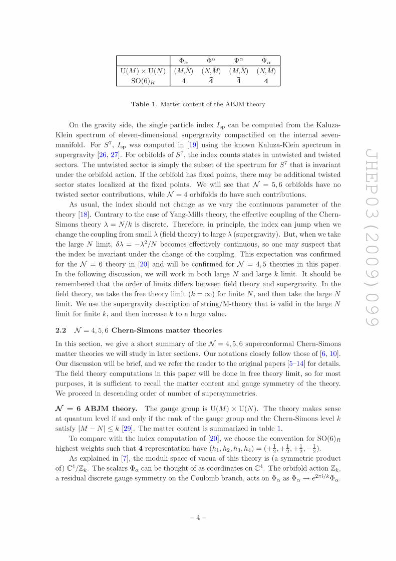
Φα Φα Ψα Ψα

U(M) × U(N) (M,N) (N,M) (M,N) (N,M)

SO(6)R 4 4 4 4

Table 1. Matter content of the ABJM theory

On the gravity side, the single particle index Isp can be computed from the Kaluza-

Klein spectrum of eleven-dimensional supergravity compactified on the internal seven-

manifold. For S7, Isp was computed in [19] using the known Kaluza-Klein spectrum in

supergravity [26, 27]. For orbifolds of S7, the index counts states in untwisted and twisted

sectors. The untwisted sector is simply the subset of the spectrum for S7 that is invariant

under the orbifold action. If the orbifold has fixed points, there may be additional twisted

sector states localized at the fixed points. We will see that N = 5, 6 orbifolds have no

twisted sector contributions, while N = 4 orbifolds do have such contributions.

As usual, the index should not change as we vary the continuous parameter of the

theory [18]. Contrary to the case of Yang-Mills theory, the effective coupling of the Chern-

Simons theory λ = N/k is discrete. Therefore, in principle, the index can jump when we

change the coupling from small λ (field theory) to large λ (supergravity). But, when we take

the large N limit, δλ = −λ2/N becomes effectively continuous, so one may suspect that

the index be invariant under the change of the coupling. This expectation was confirmed

for the N = 6 theory in [20] and will be confirmed for N = 4, 5 theories in this paper.

In the following discussion, we will work in both large N and large k limit. It should be

remembered that the order of limits differs between field theory and supergravity. In the

field theory, we take the free theory limit (k = ∞) for finite N , and then take the large N

limit. We use the supergravity description of string/M-theory that is valid in the large N

limit for finite k, and then increase k to a large value.

2.2 N = 4, 5, 6 Chern-Simons matter theories

In this section, we give a short summary of the N = 4, 5, 6 superconformal Chern-Simons

matter theories we will study in later sections. Our notations closely follow those of [6, 10].

Our discussion will be brief, and we refer the reader to the original papers [5–14] for details.

The field theory computations in this paper will be done in free theory limit, so for most

purposes, it is sufficient to recall the matter content and gauge symmetry of the theory.

We proceed in descending order of number of supersymmetries.

N = 6 ABJM theory. The gauge group is U(M) × U(N). The theory makes sense

at quantum level if and only if the rank of the gauge group and the Chern-Simons level k

satisfy |M −N | ≤ k [29]. The matter content is summarized in table 1.

To compare with the index computation of [20], we choose the convention for SO(6)Rhighest weights such that 4 representation have (h1, h2, h3, h4) = (+1

2 ,+12 ,+

12 ,−1

2).

As explained in [7], the moduli space of vacua of this theory is (a symmetric product

of) C4/Zk. The scalars Φα can be thought of as coordinates on C

4. The orbifold action Zk,

a residual discrete gauge symmetry on the Coulomb branch, acts on Φα as Φα → e2πi/kΦα.

– 4 –

JHEP03(2009)099

N = 5 theory. The gauge group is O(M) × Sp(2N).2 Let us denote the generators of

O(M) and Sp(2M) as Mab and Mab, respectively. The invariant anti-symmetric tensor of

Sp(2M) is denoted by ωab. The invariant tensor of Sp(4) = SO(5)R is denoted by Cαβ . We

denote the bi-fundamental matter fields by

Φaaα , Ψaa

α . (2.6)

They obey the reality condition of the form

Φαaa = (Φaa

α )† = δabωabCαβΦbb

β , (2.7)

and similarly for the fermions.

As explained in [10], the moduli space of vacua of this theory is C4/Dk where Dk is

the binary dihedral group with 4k elements. The dihedral group is generated by

α : Φα → eπi/kΦα , β : Φα → CαβΦβ . (2.8)

N = 4 quiver theories. We use (α, β; α, β) doublet indices for the SU(2)L ×SU(2)R R-

symmetry group. We denote the invariant tensors by ǫαβ, ǫαβ and their inverses by ǫαβ, ǫαβ

such that ǫαγǫγβ = δαβ , ǫαγǫγβ = δα

β. The hyper-multiplets are denoted by (qα, ψα) and the

twisted hyper-multiplets by (qα, ψα). A doublet of SU(2)L has the SO(4) highest weight

(h1, h2) = (12 ,

12 ) and a doublet of SU(2)R has (1

2 ,−12).

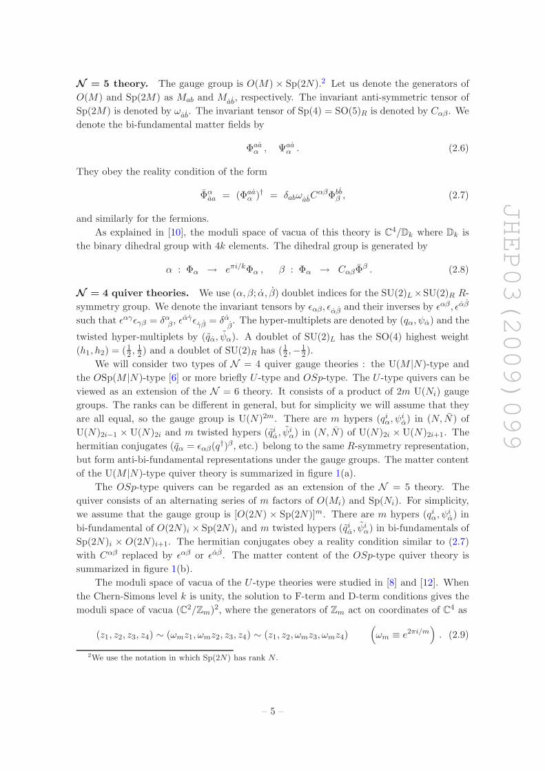
We will consider two types of N = 4 quiver gauge theories : the U(M |N)-type and

the OSp(M |N)-type [6] or more briefly U -type and OSp-type. The U -type quivers can be

viewed as an extension of the N = 6 theory. It consists of a product of 2m U(Ni) gauge

groups. The ranks can be different in general, but for simplicity we will assume that they

are all equal, so the gauge group is U(N)2m. There are m hypers (qiα, ψ

iα) in (N, N) of

U(N)2i−1 × U(N)2i and m twisted hypers (qiα, ψ

iα) in (N, N) of U(N)2i × U(N)2i+1. The

hermitian conjugates (qα = ǫαβ(q†)β , etc.) belong to the same R-symmetry representation,

but form anti-bi-fundamental representations under the gauge groups. The matter content

of the U(M |N)-type quiver theory is summarized in figure 1(a).

The OSp-type quivers can be regarded as an extension of the N = 5 theory. The

quiver consists of an alternating series of m factors of O(Mi) and Sp(Ni). For simplicity,

we assume that the gauge group is [O(2N) × Sp(2N)]m. There are m hypers (qiα, ψ

iα) in

bi-fundamental of O(2N)i × Sp(2N)i and m twisted hypers (qiα, ψ

iα) in bi-fundamentals of

Sp(2N)i × O(2N)i+1. The hermitian conjugates obey a reality condition similar to (2.7)

with Cαβ replaced by ǫαβ or ǫαβ. The matter content of the OSp-type quiver theory is

summarized in figure 1(b).

The moduli space of vacua of the U -type theories were studied in [8] and [12]. When

the Chern-Simons level k is unity, the solution to F-term and D-term conditions gives the

moduli space of vacua (C2/Zm)2, where the generators of Zm act on coordinates of C4 as

(z1, z2, z3, z4) ∼ (ωmz1, ωmz2, z3, z4) ∼ (z1, z2, ωmz3, ωmz4)(ωm ≡ e2πi/m

). (2.9)

2We use the notation in which Sp(2N) has rank N .

– 5 –

JHEP03(2009)099

U(N)2i−1 U(N)2i U(N)2i+1

qiα

qiα

¯qiα

qiα

qi+1α

qi−1

α

¯qi−1

αqi+1

α

(a)

(b)qi

αqi

αqi+1

αqi−1

α

O(2N)i O(2N)i+1Sp(2N)i

Figure 1. Matter content of (a) U -type and (b) OSp-type quiver theories.

For k > 1, as in the N = 6 theory, the residual discrete gauge symmetry induces further

orbifolding by

(z1, z2, z3, z4) ∼ ωk(z1, z2, z3, z4) . (2.10)

Note that all the orbifold actions (2.9), (2.10) can be generated by two (as opposed to

three) generators. In the simple case where m and k are relatively prime, we may choose

the independent generators to be

(ωm, ωm, 1, 1) and (ωmk, ωmk, ωmk, ωmk) , (2.11)

and say that the moduli space is C4/(Zm ×Zmk). Similarly, the moduli space of the OSp-

type theories can be shown to be (C2/Zm)2/Dk ≃ C4/(Zm ×Dmk). The orbifold action Zm

is the same as (2.9) and the action of Dk is the same as in the N = 5 theory.

For later purposes, let us review some details of the supersymmetry algebra of the

N = 4 theories. We denote the supercharges by Qαα and write their components as Q±±.

The matter fields can be written as q±, ψ± and so on. In this notation, the special super-

charge involved in the definition of the superconformal index is Q++. The supersymmetry

transformation rule includes

[Q++, q

i+

]= 0 ,

[Q−+, q

i+

]= ψi

+ ,[Q++, ψ

i+

]= qi

+qi+1+ qi+1

+ − qi+q

i+q

i+ . (2.12)

and similar relations obtained by hermitian conjugation and/or exchange of hypers with

twisted hypers.

2.3 Indices for N = 6 ABJM theories

We now review the computation of the index of the N = 6 theory following [20].3 We will

be slightly more general and allow the gauge group to be U(M) × U(N). The compact

3 The same index was computed in [21] using a different method of evaluating the integral (2.16). The

same reference also gives general formulas for the index for superconformal algebra OSp(2N |4). See also

a related work [28] where the indices of SO/Sp gauge theories (in four dimensions) were computed, which

complements the method we develop in the next section.

– 6 –

JHEP03(2009)099

bosonic subgroup of the superconformal group is SO(2)× SO(3)× SO(6), and the index is

given by

I(x, y1, y2) = Tr((−1)Fxǫ0+jyh2

1 yh32

), (2.13)

where hi’s are the second and third Cartan charges of SO(6). The single letter index for

bi-fundamental and anti-bi-fundamental matter fields are

f12 =x1/2

1 − x2

(√y1

y2+

√y2

y1

)− x3/2

1 − x2

(√y1y2 +

1√y1y2

), (2.14)

f21 =x1/2

1 − x2

(√y1y2 +

1√y1y2

)− x3/2

1 − x2

(√y1

y2+

√y2

y1

). (2.15)

On the field theory side, the superconformal index is given by

I =

∫DU1DU2 exp

∑

a,b

∞∑

n=1

1

nfab (xn, yn

1 , yn2 )Tr (Un

a ) Tr(U †n

b

) . (2.16)

The only difference from [20] is that now U2 is an element of U(M). Now, we make the

change of variables in a standard way in large N computations,

ρn =1

NTrUn

1 , χn =1

MTrUn

2 . (2.17)

Then the measure is given by (a derivation of this measure factor is given in appendix A)

DU1 =

∞∏

n=1

dρn exp

(−N2

∑

n

ρnρ−n

n

), (2.18)

DU2 =

∞∏

n=1

dχn exp

(−M2

∑

n

χnχ−n

n

). (2.19)

Substituting this, and writing M = N +m, we get

I =∏

n

dρndχn exp

(−N

2

2

∑

n

1

nCT

nMnCn

). (2.20)

Here, CTn = (χn ρn χ−n ρ−n) and

Mn =

0 0 (1 + α)2 −(1 + α)f21;n

0 0 −(1 + α)f12;n 1

(1 + α)2 −(1 + α)f12;n 0 0

−(1 + α)f21;n 1 0 0

, (2.21)

with α = m/N and fab;n ≡ fab(xn, yn

1 , yn2 ). The overall normalization of the Gaussian

integral is fixed by requiring that I(x = 0, yi = 0) = 1. The final result is

I =∏

n

(1 + α)2√detMn

=∏

n

(1 − x2n

)2(1 − xn

yn1

)(1 − xn

yn2

)(1 − xnyn

1 ) (1 − xnyn2 ),

Isp =x

y1 − x+

1

1 − xy1+

x

y2 − x+

1

1 − xy2− 2

1 − x2. (2.22)

– 7 –

JHEP03(2009)099

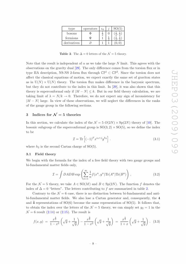
type operators ǫ0 j SO(5)

bosons Φ 12 0 (1

2 ,12)

fermions Ψ 1 12 (1

2 ,12)

derivatives ∂ 1 1 (0, 0)

Table 2. The ∆ = 0 letters of the N = 5 theory.

Note that the result is independent of α as we take the large N limit. This agrees with the

observations on the gravity dual [29]. The only difference comes from the torsion flux or in

type IIA description, NS-NS 2-form flux through CP1 ⊂ CP

3. Since the torsion does not

affect the classical equations of motion, we expect exactly the same set of graviton states

as in U(N) × U(N) theory. The torsion flux makes difference in the baryonic spectrum,

but they do not contribute to the index in this limit. In [29], it was also shown that this

theory is superconformal only if |M −N | ≤ k. But in our field theory calculation, we are

taking limit of λ = N/k → 0. Therefore, we do not expect any sign of inconsistency for

|M −N | large. In view of these observations, we will neglect the differences in the ranks

of the gauge group in the following sections.

3 Indices for N = 5 theories

In this section, we calculate the index of the N = 5 O(2N) × Sp(2N) theory of [10]. The

bosonic subgroup of the superconformal group is SO(3, 2) × SO(5), so we define the index

to be

I = Tr[(−1)Fxǫ0+jyh2

]. (3.1)

where h2 is the second Cartan charge of SO(5).

3.1 Field theory

We begin with the formula for the index of a free field theory with two gauge groups and

bi-fundamental matter fields only,

I =

∫DADB exp

(∞∑

n=1

1

nf(xn, yn)Tr(An)Tr(Bn)

), (3.2)

For the N = 5 theory, we take A ∈ SO(M) and B ∈ Sp(2N). The function f denotes the

index of ∆ = 0 “letters”. The letters contributing to f are summarized in table 2.

Contrary to the N = 6 case, there is no distinction between bi-fundamental and anti-

bi-fundamental matter fields. We also lose a Cartan generator and, consequently, the 4

and 4 representations of SO(6) become the same representation of SO(5). It follows that,

to obtain the index over the letters of the N = 5 theory, we can simply set y2 = 1 in the

N = 6 result (2.14) or (2.15). The result is

f(x, y) =x

12

1 − x2

(√y +

1√y

)− x

32

1 − x2

(√y +

1√y

)=

x12

1 + x

(√y +

1√y

). (3.3)

– 8 –

JHEP03(2009)099

Integration measure

SO(2N). Any element A ∈ SO(2N) can be block-diagonalized into the form

A =N⊕

i=1

(cosαi − sinαi

sinαi cosαi

)(|αi| ≤ π) . (3.4)

In this basis, the Harr measure over the SO(2N) group manifold is (see appendix A)

DA =N∏

i=1

dαi

∏

i<j

sin2

(αi − αj

2

)sin2

(αi + αj

2

). (3.5)

Throughout this subsection, we will suppress unimportant overall normalization constants.

In the large N limit, we can introduce the eigenvalue distribution function

ρ(θ) =∑

i

δ(θ − αi). (3.6)

Since the “eigenvalues” of SO(2N) come in pairs (e±αi), we can choose αi > 0 without loss

of generality and restrict the domain of ρ(θ) to be [0, π], so that

∫ π

0ρ(θ)dθ = N. (3.7)

Now, instead of integrating over αi’s we can integrate over the Fourier modes of ρ:

ρ(θ) =1

π

1

2ρ0 +

∑

n≥1

ρn cos(nθ)

, ρn = 2

∫ π

0ρ(θ) cos(nθ)dθ . (3.8)

The normalization of ρn is chosen such that4

Tr(An) = 2∑

i

cos(nαi) = 2

∫dθρ(θ) cos(nθ) = ρn . (3.9)

We can rewrite the measure factor as

DA =∏

i

dαi exp

∑

i<j

(log

∣∣∣∣sin2

(αi − αj

2

)∣∣∣∣+ log

∣∣∣∣sin2

(αi + αj

2

)∣∣∣∣)

=∏

i

dαi exp

−2

∞∑

n=1

∑

i<j

(cos(n(αi − αj))

n+

cos(n(αi + αj))

n

) (3.10)

=∏

i

dαi exp

−

∞∑

n=1

∑

i,j

(cos(n(αi − αj))

n+

cos(n(αi + αj))

n

)−∑

i

cos(2nαi)

n

.

4The normalization here differs from that in (2.17) by a factor of N . This is to emphasize that the finite

shift in (3.13) survives the large N limit.

– 9 –

JHEP03(2009)099

In the large N limit,

∑

i,j

(cos(n(αi − αj))

n+

cos(n(αi + αj))

n

)

→∫dθ1dθ2ρ(θ1)ρ(θ2)

(cos(n(θ1 − θ2))

n+

cos(n(θ1 + θ2)

n

)=

1

2nρ2

n, (3.11)

∑

i

cos(2nαi)

n→∫dθρ(θ)

cos(2nθ)

n=

1

2nρ2n . (3.12)

To summarize, the integration measure of SO(2N) is

DA =∏

m

dρm exp

(−∑

n odd

1

2nρ2

n −∑

n even

1

2n(ρn − 1)2

). (3.13)

This measure is consistent with the fact that

〈trA2k+1〉 = 0, 〈trA2k〉 = 1, (3.14)

which holds exactly (without large N approximation) for 2k < N .

SO(2N+1). The discussion proceeds in parallel with that of SO(2N) with two important

differences. First, the Harr measure over the SO(2N + 1) group manifold is given by

DA =

N∏

i=1

dαi

∏

i<j

sin2

(αi − αj

2

)sin2

(αi + αj

2

)∏

i

sin2(αi

2

). (3.15)

The last factor∏

i sin2(αi/2) induces a linear term in ρn for every (even and odd) n.

However, this shift is precisely compensated by another shift in the definition of ρn,

ρn ≡ tr(An) = 2∑

i

cos(nαi) + 1 . (3.16)

As a result, the final form of the measure of SO(2N + 1) in the large N limit is identical

to that of SO(2N) in (3.13).

Sp(2N). The Harr measure over the Sp(2N) group manifold is given by

DB =N∏

i=1

dβi

∏

i<j

sin2

(βi − βj

2

)sin2

(βi + βj

2

)∏

i

sin2 βi, . (3.17)

Compared to the SO(2N) case, the∏

i sin2 βi term over-compensates the shifts for n =

2k, resulting in the net shift +1 as opposed to −1 of SO(2N). In other words, with

the definition,

χn ≡ tr(Bn) = 2∑

i

cos(nβi) , (3.18)

the integration measure is given by

DB =∏

m

dχm exp

(−∑

n odd

1

2nχ2

n −∑

n even

1

2n(χn + 1)2

). (3.19)

– 10 –

JHEP03(2009)099

Result. In terms of the shorthand notation, fn ≡ f(xn, yn), the index to be computed is

I =

∫DADB exp

(∞∑

n=1

1

nfnρnχn

), (3.20)

where the integration measures are given in (3.13) and (3.19). Performing the Gaussian

integral by diagonalization (ρ±n = ρn ± χn), we obtain

I =

∞∏

n=1

1√1 − f2

n

∞∏

k=1

exp

(− f2k

2k(1 + f2k)

). (3.21)

The overall normalization is fixed by requiring that I(x = y = 0) = 1. Using the relations,

1

1 − f2n

=(1 + xn)2

(1 − (xy)n)(1 − (x/y)n),

f2k

1 + f2k=

(xy)k + (x/y)k

(1 + (xy)k)(1 + (x/y)k), (3.22)

we can exponentiate the∏

(1 − f2n)−1/2 factor and rewrite the result as

I = exp

(∞∑

k=1

1

kIsp

(xk, yk

)),

Isp =x

1 − x2+

1

2

[xy

1 − xy+

x/y

1 − x/y− xy + x/y

(1 + xy)(1 + x/y)

]

=1

1 − x2

[(1 − x/y)

(xy)2

1 − (xy)2+ (1 − xy)

(x/y)2

1 − (x/y)2+ x+ x2

]. (3.23)

3.2 Gravity

The gravity computation can be done by taking the states of AdS4 × S7 and keeping

the states invariant under the orbifold action. The spectrum of AdS4 × S7 was originally

obtained in [26, 27] and recently discussed in the context of the superconformal index

in [19]. The Zk orbifolding was studied in [20]. In the basis where the supercharges

transform vectorially under the SO(8), the Zk action is a rotation by 4π/k along the SO(2)

part of the decomposition SO(6)×SO(2) ⊂ SO(8). If we denote the generator of the SO(2)

by J3, then the invariant states should satisfy

exp

(4πi

kJ3

)|ψ〉 = 0 , (3.24)

which means J3|ψ〉 = 0 for large k.

The Dk group is a subgroup of the SO(3) in the decomposition SO(5)×SO(3) ⊂ SO(8).

If we denote the SO(3) generators by J1,2,3, the generators of Dk are given by

exp

(2πi

kJ3

), exp (πiJ2) . (3.25)

For large k, the first generator again requires that J3|ψ〉 = 0. In the standard |ℓ,m〉notation, all |ℓ ∈ Z,m = 0〉 states satisfy this condition. They are also eigenstates of

– 11 –

JHEP03(2009)099

range of n ǫ0 j SO(8)

n ≥ 1 n2 0 (n

2 ,n2 ,

n2 ,

−n2 )

n ≥ 1 n+12

12 (n

2 ,n2 ,

n2 ,

−(n−2)2 )

n ≥ 2 n+22 1 (n

2 ,n2 ,

(n−2)2 , −(n−2)

2 )

n ≥ 2 n+32

32 (n

2 ,(n−2)

2 , (n−2)2 , −(n−2)

2 )

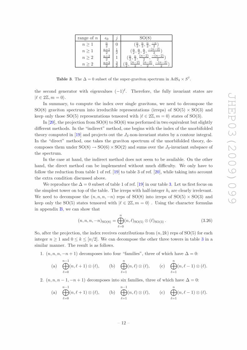
Table 3. The ∆ = 0 subset of the super-graviton spectrum in AdS4 × S7.

the second generator with eigenvalues (−1)ℓ. Therefore, the fully invariant states are

|ℓ ∈ 2Z,m = 0〉.In summary, to compute the index over single gravitons, we need to decompose the

SO(8) graviton spectrum into irreducible representations (irreps) of SO(5) × SO(3) and

keep only those SO(5) representations tensored with |ℓ ∈ 2Z,m = 0〉 states of SO(3).

In [20], the projection from SO(8) to SO(6) was performed in two equivalent but slightly

different methods. In the “indirect” method, one begins with the index of the unorbifolded

theory computed in [19] and projects out the J3-non-invariant states by a contour integral.

In the “direct” method, one takes the graviton spectrum of the unorbifolded theory, de-

composes them under SO(8) → SO(6)× SO(2) and sums over the J3-invariant subspace of

the spectrum.

In the case at hand, the indirect method does not seem to be available. On the other

hand, the direct method can be implemented without much difficulty. We only have to

follow the reduction from table 1 of ref. [19] to table 3 of ref. [20], while taking into account

the extra condition discussed above.

We reproduce the ∆ = 0 subset of table 1 of ref. [19] in our table 3. Let us first focus on

the simplest tower on top of the table. The irreps with half-integer hi are clearly irrelevant.

We need to decompose the (n, n, n,−n) reps of SO(8) into irreps of SO(5) × SO(3) and

keep only the SO(5) states tensored with |ℓ ∈ 2Z,m = 0〉 . Using the character formulas

in appendix B, we can show that

(n, n, n,−n)SO(8) =

n⊕

ℓ=0

(n, ℓ)SO(5) ⊗ (ℓ)SO(3) . (3.26)

So, after the projection, the index receives contributions from (n, 2k) reps of SO(5) for each

integer n ≥ 1 and 0 ≤ k ≤ [n/2]. We can decompose the other three towers in table 3 in a

similar manner. The result is as follows.

1. (n, n, n,−n+ 1) decomposes into four “families”, three of which have ∆ = 0:

(a)n−1⊕

ℓ=0

(n, ℓ+ 1) ⊗ (ℓ), (b)n⊕

ℓ=1

(n, ℓ) ⊗ (ℓ), (c)n⊕

ℓ=1

(n, ℓ− 1) ⊗ (ℓ).

2. (n, n, n− 1,−n+ 1) decomposes into six families, three of which have ∆ = 0:

(a)

n−1⊕

ℓ=0

(n, ℓ+ 1) ⊗ (ℓ), (b)

n−1⊕

ℓ=1

(n, ℓ) ⊗ (ℓ), (c)

n⊕

ℓ=1

(n, ℓ− 1) ⊗ (ℓ).

– 12 –

JHEP03(2009)099

3. (n, n− 1, n− 1,−n + 1) decomposes into four families, one of which has ∆ = 0:

n−1⊕

ℓ=0

(n, ℓ) ⊗ (ℓ).

Now, it is easy to sum over all SO(5) reps with ℓ =(even). Introduce the notation,

Q1 ≡∞∑

k=0

χ(2k)SO(3)(y)

∞∑

m=0

xm+2k =1

(1 − x)(1 − y)

[1

1 − x2/y2− y

1 − x2y2

], (3.27)

Q2 ≡∞∑

k=0

χ(2k+1)SO(3) (y)

∞∑

m=0

xm+2k =1

(1 − x)(1 − y)

[y−1

1 − x2/y2− y2

1 − x2y2

]. (3.28)

Then, the partial sums

Sj =∑

xǫ0+jχ(h)SO(3)(y) , (3.29)

can be written as

S0 = Q1 − 1 ,

S(a)1/2 = x2Q2 , S

(b)1/2 = x

(Q1 −

1

1 − x

), S

(c)1/2 = x3Q2 ,

S(a)1 = x3Q2 , S

(b)1 = x3

(Q1 −

1

1 − x

), S

(c)1 = x4Q2 ,

S3/2 = x4Q1 . (3.30)

To sum up, the index evaluated over all single gravitons is

Isp =1

1 − x2

∑

j

(−1)2jSj .

=1

1 − x2

[(1 − x/y)

(xy)2

1 − (xy)2+ (1 − xy)

(x/y)2

1 − (x/y)2+ x+ x2

], (3.31)

in perfect agreement with the field theory result (3.23).

4 Indices for N = 4 theories

4.1 U-type

Field theory. Since the R-symmetry group is SO(4), we define the index to be

I(x, y) = Tr[(−1)Fxǫ0+jyh2

]. (4.1)

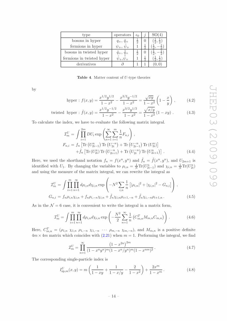
where h2 is the second Cartan charge of SO(4). We can read off the letters contributing to

the single-letter partition function f from the matter content in figure 1(a).

The result is summarized in table 4. Then, the single letter partition function is given

– 13 –

JHEP03(2009)099

type operators ǫ0 j SO(4)

bosons in hyper q+, q+12 0 (1

2 ,12)

fermions in hyper ψ+, ψ+ 1 12 (1

2 ,−12)

bosons in twisted hyper q+, ¯q+12 0 (1

2 ,−12)

fermions in twisted hyper ψ+,¯ψ+ 1 1

2 (12 ,

12)

derivatives ∂ 1 1 (0, 0)

Table 4. Matter content of U -type theories

by

hyper : f(x, y) =x1/2y1/2

1 − x2− x3/2y−1/2

1 − x2=

√xy

1 − x2

(1 − x

y

), (4.2)

twisted hyper : f(x, y) =x1/2y−1/2

1 − x2− x3/2y1/2

1 − x2=

√x/y

1 − x2(1 − xy) . (4.3)

To calculate the index, we have to evaluate the following matrix integral.

IUm =

∫ 2m∏

i=1

DUi exp

(∞∑

n=1

m∑

i=1

1

nFn,i

),

Fn,i = fn

[Tr(Un

2i−1

)Tr(U−n

2i

)+ Tr

(U−n

2i−1

)Tr (Un

2i)]

+fn

[Tr (Un

2i)Tr(U−n

2i+1

)+ Tr

(U−n

2i

)Tr(Un

2i+1

)]. (4.4)

Here, we used the shorthand notation fn = f(xn, yn) and fn = f(xn, yn), and U2m+1 is

identified with U1. By changing the variables to ρi,n = 1N Tr(Un

2i−1) and χi,n = 1N Tr(Un

2i)

and using the measure of the matrix integral, we can rewrite the integral as

IUm =

∫ m∏

i=1

∞∏

n=1

dρi,ndχi,n exp

−N2

∑

i,n

1

n

[|ρi,n|2 + |χi,n|2 −Gn,i

] ,

Gn,i = fnρi,nχi,n + fnρi,−nχi,n + fnχi,nρi+1,−n + fnχi,−nρi+1,n . (4.5)

As in the N = 6 case, it is convenient to write the integral in a matrix form,

IUm =

∫ m∏

i=1

∞∏

n=1

dρi,ndχi,n exp

(−N

2

2

∞∑

n=1

1

n

(CT

m,nMm,nCm,n

)). (4.6)

Here, CTm,n = (ρ1,n χ1,n ρ1,−n χ1,−n · · · ρm,−n χm,−n), and Mm,n is a positive definite

4m× 4m matrix which coincides with (2.21) when m = 1. Performing the integral, we find

IUm =

∞∏

n=1

(1 − x2n

)2m

(1 − xnyn)m(1 − xn/yn)m(1 − xnm)2. (4.7)

The corresponding single-particle index is

IUsp,m(x, y) = m

(1

1 − xy+

1

1 − x/y− 2

1 − x2

)+

2xm

1 − xm. (4.8)

– 14 –

JHEP03(2009)099

Gravity. The gravity computation in the untwisted sector turns out to be almost trivial.

The orbifolding action due to the Chern-Simons level (in the k → ∞ limit) makes the same

effect as in the process of going from N = 8 to N = 6. Thus, we can begin with the N = 6

single-particle index

IN=6sp (x, y1, y2) =

x

y1 − x+

1

1 − xy1+

x

y2 − x+

1

1 − xy2− 2

1 − x2. (4.9)

The other Zm orbifolding acts only on y2. So, we can simply take

IUsp,m(x, y) =

1

m

m∑

j=1

IN=6sp

(x, y, ωj

m

)=

1

1 − xy+

1

1 − x/y− 2

1 − x2+

2xm

1 − xm.(4.10)

Comparing (4.10) and (4.8), we find a mismatch

∆IUsp,m = (m− 1)

(1

1 − xy+

1

1 − x/y− 2

1 − x2

)

= (m− 1)1

1 − x2

((1 − x/y)

xy

1 − xy+ (1 − xy)

x/y

1 − x/y

). (4.11)

We will now argue that the twisted sector contributions can account for the mismatch and

lead to perfect agreement of the index between field theory and gravity.

Twisted sector — field theory. Suppose we have operators O(i) (i = 1, · · · ,m) which

form a regular representation of Zm. Then, the (m − 1) linearly independent operators

O(i+ 1) −O(i) not invariant under Zm must belong to the twisted sector.

The bosonic single-trace operators that contribute to the index are given by

OBn (i) = Tr

(qi+q

i+

)n, OB

n (i) = Tr(qi+

¯qi+

)n, (4.12)

where qi are hypers in (N, N ) of U(N)2i−1 and U(N)2i, and qis are twisted hypers in (N, N )

of U(N)2i × U(N)2i+1. The bars denote hermitian conjugation. As explained earlier, the

subscripts (±) denote the doublet indices under the SU(2)L × SU(2)R R-symmetry.

The supersymmetry transformation rule (2.12) shows that these operators are annihi-

lated by Q++ and S−− = (Q++)†, so they contribute to the index. Their quantum numbers

are (ǫ0, j, h1, h2) = (n, 0, n,±n), so ∆ = ǫ0 − j − h1 = 0 as expected.

To obtain the fermionic operators, we can take the super-descendants of the bosonic

operators by acting with supercharges commuting with Q++. We find

OFn (i) =

[Q−+, O

Bn (i)

]= Tr

[(ψi

+qi+ + qi

+ψi+

) (qi+q

i+

)n−1],

OFn (i) =

[Q+−, O

Bn (i)

]= Tr

[(ψi

+¯qi+ + qi

+¯ψi

+

) (qi+

¯qi+

)n−1], (4.13)

whose quantum numbers are (ǫ0, j, h1, h2) = (n + 1/2, 1/2, n,±(n − 1)) such that ∆ = 0.

The superconformal algebra,

Q++, Q±∓ = 0, S−−, Q−+ ∝ J−−, S−−, Q+− ∝ J−−, (4.14)

– 15 –

JHEP03(2009)099

where J and J are generators of SU(2)L × SU(2)R, shows that these fermionic operators

are also annihilated by Q++ and S−− and contribute to the index. Taking into account the

bosonic descendants (derivatives), we obtain the index summed over the Zm non-invariant

bosonic and fermionic operators,

IUsp,m(twisted) = (m− 1) × 1

1 − x2

[(1 − x/y)

xy

1 − xy+ (1 − xy)

x/y

1 − x/y

], (4.15)

which agrees precisely with the mismatch (4.11).

It is rather remarkable that (4.12) and (4.13) exhaust all twisted sector contributions

to the index, as there are many more operators which apparently satisfy ∆ = 0. However,

all such operators connecting three or more nodes of the quiver can be shown to be (Q++)-

exact by using the supersymmetry transformation rule (2.12). For instance, repeated use

of (2.12) shows that

O(i) = Tr(qi+q

i+q

i+q

i+

¯qi+q

i+

),

O(i+ 1) −O(i) =[Q++,Tr

(qi+1+ qi+1

+ qi+1+ ψi+1

+ + qi+1+ qi+1

+¯ψi+q

i + ¯ψi+q

i+q

i+q

i+

)].(4.16)

In the N = 2 superfield language adopted in [8, 12], this is a consequence of the F-term

equivalence relations.

Twisted sector — gravity. The field theory computation above implies that there

should be corresponding twisted sector states on the gravity side. In fact, the orbifold

has two copies of S2 ⊂ CP3 ⊂ S7 as the fixed loci, one at (z1, z2, 0, 0) and the other at

(0, 0, z3, z4), as the circle fiber of the Hopf fibration of S3 is removed by the Zmk orbifold

action in the large k limit. Therefore, in type IIA description, there should exist chiral

primary states in the twisted sector localized at these fixed loci. Note that the splitting of

twisted sector states into hypers and twisted hypers as in (4.12) and (4.13) matches nicely

with two disjoint fixed loci of the orbifold geometry.

To understand the nature of the twisted sector states, let us examine the geometry

near the fixed loci. We begin with writing the metric of S7 as

ds2 = dα2 + sin2 αdΩ21 + cos2 αdΩ2

2

= dα2 +1

4sin2 α

[dθ2

1 + sin2 θ1dφ21 + (dψ1 + cos θ1dφ1)

2]

+1

4cos2 α

[dθ2

2 + sin2 θ2dφ22 + (dψ2 + cos θ2dφ2)

2]. (4.17)

The orbifold action can be taken to be

(ψ1, ψ2) ∼ (ψ1 + 2π/m,ψ2) ∼ (ψ1 + 2π/mk,ψ2 + 2π/mk) . (4.18)

Near α = 0, it is convenient to take the “fundamental domain” of the (ψ1, ψ2) torus

as follows:

ψ1 = ψ + β, ψ2 = ψ, 0 < ψ < 2π/mk, 0 < β < 2π/m. (4.19)

– 16 –

JHEP03(2009)099

Then the metric can be rewritten as

ds2 = dα2 +1

4sin2 α

(dθ2

1 + sin2 θ1dφ21

)+

1

4cos2 α

(dθ2

2 + sin2 θ2dφ22

)

+1

4cos2 α sin2 α(dβ + cos θ1dφ1 − cos θ2dφ2)

2

+1

4

[dψ + sin2 α(dβ + cos θ1dφ1) + cos2 α cos θ2dφ2

]2

≈ dα2 +1

4α2[dθ2

1 + sin2 θ1dφ21 + (dβ + cos θ1dφ1 − cos θ2dφ2)

2]

+1

4

(dθ2

2 + sin2 θ2dφ22

)+

1

4[dψ + · · · ]2 . (4.20)

The angle ψ is the coordinate of the 11-th circle. So, up to an overall warping, the IIA

metric near the singularity looks like a non-trivial fibration of Am−1 over S2.

A direct string theoretic analysis of the twisted sector states would be a formidable

task. Instead, we could follow the analysis of [30] where blow-up of the orbifold was used to

obtain the spectrum of the twisted sector states. There are (m−1) normalizable harmonic

two-forms ωi in the blown-up Am−1 singularity. As in [30], the candidate for chiral primary

states in the twisted sector comes from the harmonic decomposition of the NSNS B-field

into (m− 1) scalars by

B =m−1∑

i=1

φi ωi . (4.21)

The spherical harmonics on either S2 have integer “spin”-n under SU(2)L or SU(2)R fac-

tors of the SO(4) R-symmetry. In particular, the highest weight states have the SO(4)

Cartan charges (h1, h2) = (n,±n). Therefore, in order to match the quantum numbers

(ǫ0, j, h1, h2) = (n, 0, n,±n) of the twisted sector states found in the field theory, it would

be sufficient to show that these states have ǫ0 = n, which is equivalent to (mass)2 = n(n−3).

The Laplacian operator contributes n(n + 1) to the mass squared of the scalar fields. As

noted in [30], the interaction of the B-field with background RR 3-form and 1-form fields

is likely to produce a shift in mass squared. Having ǫ0 = n amounts to a mass shift

δ(mass)2 = −4n.

The computation of the mass shift would take two steps. First, we need to blow up

the metric (4.20) while maintaining the Einstein condition. Second, we solve the equation,

d ∗ dC3 =1

2dC3 ∧ dC3 , (4.22)

of eleven-dimensional supergravity with the ansatz

C3 = C3(background) + φi ωi ∧ (dψ + · · · ) . (4.23)

We leave the detailed computation of the mass shift to a future work.

4.2 OSp-type

Field theory. We have m copies of alternating O(2N) and Sp(2N) gauge groups, and

the quiver diagram is given in figure 1(b). Since the matter content is all the same as in

– 17 –

JHEP03(2009)099

the U -type theory except that they are in the real representations of the gauge group, the

single letter partition function is exactly the same as that of the U -type theory.

hyper : f(x, y) =x1/2y1/2

1 − x2− x3/2y−1/2

1 − x2=

√xy

1 − x2

(1 − x

y

), (4.24)

twisted hyper : f(x, y) =x1/2y−1/2

1 − x2− x3/2y1/2

1 − x2=

√x/y

1 − x2(1 − xy) . (4.25)

Plugging in the single letter partition functions to the matrix-integral formula for the index,

we obtain,

IOSpm =

∫ m∏

i=1

DAiDBi exp

(∞∑

n=1

m∑

i=1

1

nFn,i

),

Fn,i = fnTr(Ani )Tr(Bn

i ) + fnTr(Bni )Tr(An

i+1) , (4.26)

where fn = f(xn, yn) and A and B are elements of orthogonal and symplectic gauge group

respectively. Since we consider circular quivers, we identify Am+1 ∼ A1 and Bm+1 ∼ B1.

We can repeat the same matrix integral for N = 5 OSp theory except that there are m

copies of gauge group and matters. The result is

IOSpm =

∏

n=1

(1 − x2n)m

(1 − (xy)n)m/2(1 − (x/y)n)m/2(1 − xnm)

∏

k=1

exp

(− f2k

2k(1 + f2k)

). (4.27)

The corresponding single-particle index is

IOSpsp,m =

m

2

(1

1 − xy+

1

1 − x/y− 2

1 − x2− xy + x/y

(1 + xy)(1 + x/y)

)+

xm

1 − xm. (4.28)

For m = 1, it agrees with the N = 5 result as expected.

Gravity. Again, we can work out the decomposition of representations, etc., but there

is a shortcut. Consider the broken SO(4) = SU(2) × SU(2) ⊂ SO(8) and denote its

representations by (j1, j2). Taking the Dk orbifold action into account, but leaving the Zm

orbifolding aside, we can write down the “preliminary version” of the index as follows:

IOSp−presp,m =

∫dθ

2πtr

xǫ0+j

1 − x2yh21 yh3

2

1 + e

πin

J(1)2 +J

(2)2

o

2

e

iθn

J(1)3 +J

(2)3

o

. (4.29)

As before, the Zk orbifolding picks out only the states with m1 + m2 = 0. The other

generator of Dk acts on these states as

eπi

h

J(1)2 +J

(2)2

i

|j1, j2; +m,−m〉 = (−1)j1+j2|j1, j2;−m,+m〉 . (4.30)

The first half of (4.29) which does not involve J(1)2 + J

(2)2 is nothing but one half of the

N = 6 index. The other half (call it ∆I) picks up contributions only from the states with

m1 = m2 = 0 because of (4.30). Since h3 = m1 −m2 in (4.29), ∆I is independent of y2.

– 18 –

JHEP03(2009)099

Before the Zm orbifolding, the index must coincide with the N = 5 result.5 Therefore,

∆I(x, y) = IN=5sp (x, y) − 1

2IN=6sp (x, y, y2 = 1) . (4.31)

The Zm orbifolding acts only on y2, so it makes no effect on ∆I.

IOSpsp,m(x, y) =

1

m

m∑

j=1

IOSp−presp,1 (x, y, ωj

m) (ωm ≡ e2πi/m)

=1

2m

m∑

j=1

IN=6sp (x, y, ωj

m) + ∆I(x, y) (4.32)

=1

2

(1

1 − xy+

1

1 − x/y− 2

1 − x2− xy + x/y

(1 + xy)(1 + x/y)

)+

xm

1 − xm.

Comparing (4.28) and (4.32), we find a mismatch

∆IOSpsp,m(x, y) =

m− 1

2

(1

1 − xy+

1

1 − x/y− 2

1 − x2− xy + x/y

(1 + xy)(1 + x/y)

)

= (m− 1) × 1 − x2

[(1 − x/y)

(xy)2

1 − (xy)2+ (1 − xy)

(x/y)2

1 − (x/y)2

]. (4.33)

Twisted sector. We can repeat the same analysis as in the previous case with slight

modifications. The bosons contributing to the index are given by

OBn (i) = Tr

(qi+q

i+

)2n, OB

n (i) = Tr(qi+

¯qi+

)2n. (4.34)

Recall that q and q are related by qaa = δabωabqbb. We have q4n rather than q2n because

the trace vanishes due to the anti-symmetric tensor ωab of Sp(2N).

The fermionic operators corresponding to the index are again obtained by taking super-

descendants of the bosonic operators:

OFn (i) =

[Q−+, O

Bn (i)

]= Tr

[(ψi

+qi+ + qi

+ψi+)(qi

+qi+)2n−1

],

OFn (i) =

[Q+−, O

Bn (i)

]= Tr

[(ψi

+¯qi+ + qi

+¯ψi

+)(qi+

¯qi+)2n−1

]. (4.35)

The bosonic and fermionic operators together contribute to the index by

(m− 1) × 1

1 − x2

[(1 − x/y)

(xy)2

1 − (xy)2+ (1 − xy)

(x/y)2

1 − (x/y)2

], (4.36)

which exactly account for the difference between supergravity approximation and field

theory computation (4.33) .

On the gravity side, we again have fixed loci at (z1, z2, 0, 0) and (0, 0, z3, z4). The Dk

action zi ∼ ωkzi and (z1, z2, z3, z4) ∼ (z2,−z1, z3,−z4) make the fixed loci to be RP2 =

S2/Z2. Among the spherical harmonics on S2, only those with even n contribute. This

matches the spectrum of twisted sector states in the field theory.

5 We could reverse the logic, compute ∆I directly and give an alternative derivation of the N = 5 index,

but we will not pursue it here.

– 19 –

JHEP03(2009)099

4.3 On the dual ABJM proposal

In [23, 24], a U(N) × U(N) Chern-Simons theory with manifest N = 2 supersymmetry

and the superpotential W = [φ1, φ2]AB was proposed, where φ1, φ2 are adjoints in the first

gauge group and A,B are bi-fundamentals. The moduli space of vacua was claimed to be

C2/Zk ×C

2, which suggests that the theory may exhibit N = 4 at the IR fixed point. The

existence of non-trivial fixed point for N = 2 Chern-Simons-Matter theories were shown

in [4]. The moduli space seems to imply that the IR fixed point of this theory is dual to

M-theory on AdS4 × S7/Zk where the Zk acts on either ψ1 or ψ2 in (4.17). For k = 1, the

moduli space is C4, and the authors of [23, 24] claim that the theory flow to the same IR

fixed point as the ABJM theory for k = 1 (hence the name “dual ABJM”). It would be

interesting to test whether the fixed point theory actually has N = 4 supersymmetry when

k > 1. For this purpose, we will compute the index on both sides and make comparison.

All the field theory computations in previous sections were based on the fact that

we can take the free theory limit by continuous marginal deformation. The free theory

computation cannot be justified if the theory undergoes a non-trivial RG flow. However,

the analysis [4] of the RG fixed point of N = 2 theories with quartic superpotential indicates

that the coefficient of the superpotential at the fixed point is of order 1/k. So, in the large k

limit, the theory is weakly coupled throughout the RG-flow and the free theory computation

may be reliable. We will proceed to perform the free theory computation and check the

consistency of the approach a posteriori.

Gravity. As usual, in the N = 8 setup before orbifolding, we take the basis of SO(8)

such that the supercharge Q has highest weight (1, 0, 0, 0) and the scalar field has highest

weight (1/2, 1/2, 1/2,−1/2). Let’s denote the 7-sphere to be

S7 =

(x1, · · · , x8)|

8∑

i=1

|xi|2 = 1

. (4.37)

Consider the Zk orbifolding action by

exp

(2π

k(H56 +H78)

), (4.38)

where H56,H78 denotes rotation generators in x5 − x6 and x7 − x8 planes. Clearly, the

surviving supercharges are vectors in x1,2,3,4 directions. Under SO(8), the scalar fields

decompose as

φ1 : ±1

2(+,+,+,−) ,

φ2 : ±1

2(+,+,−,+) ,

A : ±1

2(+,−,+,+) ,

B : ±1

2(+,−,−,−) . (4.39)

Note that φ1,2 are neutral under the orbifold action, while A and B have charge ±1.

– 20 –

JHEP03(2009)099

type operators ǫ0 j (h1, h2)

bosons φ1,b12 0 (1

2 ,12)

φ2,b12 0 (1

2 ,12)

Ab12 0 (1

2 ,−12)

Bb12 0 (1

2 ,−12)

fermions φ1,f 1 12 (1

2 ,−12)

φ2,f 1 12 (1

2 ,−12)

Af 1 12 (1

2 ,12)

Bf 1 12 (1

2 ,12)

derivatives ∂ 1 1 (0, 0)

Table 5. The Delta = 0 letters of the dual ABJM theory

To incorporate the effect orbifolding in the index, we can invoke the contour integral

method. Take IN=8sp (x, y1, y2, y3), set y2 = y3 = z and collect the z-independent terms by

using the contour integral. The result is (setting√x = t and

√y1 = u)

Igravitysp = −1 +

1

(1 − tu)2− 2t4

(1 − t4)(1 − tu)− t2

t2 − u2. (4.40)

Field theory. From (4.39), we can identify the letters contributing to the index as in

table 5. Here, the subscript b, f denotes the bosonic and fermionic components of the

corresponding superfield. The “indices for letters” are given by

f12 = f21 =t/u− t3u

1 − t4, f11 =

2(tu− t3/u)

1 − t4, f22 = 0 . (4.41)

The matrix integral is straightforward to compute.

IFT =

∫DU1DU2 exp

∞∑

n=1

∑

a,b

1

nfab(t

n, un)tr(Una )tr(U−n

b )

=∞∏

n=1

1

1 − f(n)11 − f

(n)12 f

(n)21

=

∞∏

n=1

(1 − t4n)2

(1 − t2n/u2n)(1 − 2tnun + 2t5nun − t6nu2n). (4.42)

Comparison. Let’s expand the index by powers of t. The field theory index is given by

IFT = 1 + 2ut +(u−2 + 6u2

)t2 +

(2u−1 + 14u3

)t3 +

(2u−4 + 4 + 34u4

)t4

+(4u−3 + 8u+ 74u5

)t5 +

(3u−6 + 10u−2 + 15u2 + 166u6

)t6 + · · · , (4.43)

and the gravity side is given by

Igravity = exp

(∞∑

k=1

1

kIgravitysp (tn, un)

)

= 1 + 2ut+(u−2 + 6u2

)t2 +

(2u−1 + 14u3

)t3 +

(2u−4 + 4 + 33u4

)t4

+(4u−3 + 8u+ 70u5

)t5 +

(3u−6 + 10u−2 + 15u2 + 149u6

)t6 + · · · , (4.44)

– 21 –

JHEP03(2009)099

The results match to a large extent, but not completely:

IFT − Igravity = u4t4 + 4u5t5 + 17u6t6 + · · · . (4.45)

Note that IFT > Igravity holds order by order and that the the orbifold has the fixed locus

S3 ⊂ S7/Zk. So, it seems possible for the twisted sector states to account for the mismatch.

It is not clear, however, why only a small number of terms survive in the k → ∞ limit. It

would be worthwhile to repeat the computation for large but finite k, where perturbation

theory is applicable, in order to fully verify the existence of the N = 4 fixed point of the

dual ABJM theory.

5 Conclusion

We have checked that the superconformal indices of N = 4, 5 Chern-Simons theories match

with those of their gravitational dual theories. This provides a non-trivial check of the

proposed dual geometry. Especially, from the fact that orbifold has fixed locus, and by

identifying the contributions from the twisted sectors, we can verify that the superconformal

theory is not dual to just supergravity, but full superstring theory. The only missing

element here is the shift of the mass spectrum due to the interaction of the background 3-

form field and 2-form field B. Also, we have computed the index for the dual ABJM model

proposed by [23]. Our computation suggests that we have to go beyond the supergravity

approximation to actually verify the claim.

In principle, the superconformal index depends both on N and k, because they deter-

mine the form of possible gauge invariant operators. Our computation was done in the

large k and large N limit. In this regime, we can use weakly coupled type IIA superstring

description. We can regard the ’t Hooft coupling λ = N/k to be effectively continuous so

that the index does not change as we go from weak coupling (free field theory) to strong

coupling (supergravity). But, the index is still discrete for finite N , so it remains to be

checked whether this index does not ‘jump’ under such deformations. In fact, the spec-

trum of chiral primaries does depend on N and k [7], so we do not expect the index to

be invariant under the change of coupling when N is finite. In addition, to properly un-

derstand the behavior of the index when the two gauge groups have different ranks, (e.g.

U(M)×U(N), M 6= N) we should look into the case of finite N . According to [29], N = 6

U(M) × U(N) Chern-Simons theory remains superconformal only if |M − N | ≤ k. To

check this, we should also investigate the finite k effect. On the gravity side, finite k effect

is easily computable for large N , where we can use supergravity approximation. It is not

clear how to go beyond the large N limit in supergravity. On the field theory side, the

loop expansion in 1/k would reveal finite k effects, and there is no fundamental difficulty

in working with finite N .6 We leave the computation of the index for finite k and/or N as

a future work.

It is possible to compute the superconformal indices for less supersymmetric Chern-

Simons theories. But, less supersymmetry means the index has fewer expansion parameters.

6 Matching of the index of finite rank gauge groups in four dimensions was previously reported in [28].

– 22 –

JHEP03(2009)099

For example, in the case of N = 2, 3 theories, we only have 1 parameter in the index. And

for N = 1 theories, it becomes an ordinary Witten index. So as we go to less supersymmetic

case, the index contains less information. Also, the gravity duals of less supersymmetric

theories are more complicated, and the KK spectrum of the compact space is not known.

However, it is worth noting that the superconformal index is invariant under any defor-

mation that preserves the special supercharges Q and S. In our examples presented here,

there is no marginal deformation preserving the same number of supersymmetry besides

the Lagrangian itself. But, there are possible deformations which preserve less supersym-

metries. In this case, we should be able to identify the corresponding deformation of the

dual geometry on the gravity side. One possible example is the N = 1 Chern-Simons the-

ory obtained from deforming the free theory limit of N = 6 ABJM theory [31]. The dual

geometry of the theory is conjectured to be the orbifolded squashed seven-sphere. Since the

free theory limit of the both theory agrees, it seems possible to construct the index which

includes the global symmetry along with superconformal algebra. Another example is the

three dimensional version of the beta-deformation preserving N = 2 supersymmetry. The

gravity dual of the beta-deformation was studied earlier in [32–34]. It would be interesting

to study the deformation in the corresponding Chern-Simons theories.

Acknowledgments

We are grateful to Seok Kim, Sungjay Lee, Hirosi Ooguri, Chang-Soon Park and Masahito

Yamazaki for helpful discussions. The work of S.L. is supported in part by the KOSEF

Grant R01-2006-000-10965-0 and the Korea Research Foundation Grant KRF-2007-331-

C00073. The work of J.S. is supported in part by DOE grant DE-FG02-92ER40701 and

Samsung Scholarship.

A Matrix integrals and measure factors

In the main text, we have to calculate the matrix integration over the Lie groups U(N),

SO(2N), Sp(2N), SO(2N + 1). Here, we present a physicist’s derivation of the measure

factors using Fadeev-Popov determinant of path integral. The computation for U(N) was

described in [25]. Suppose we compactify the theory on S1 ×S2, where the Euclidean time

runs along the thermal circle S1 with radius β. By integrating out all but the zero mode

α of the time component of the gauge field, we obtain the following effective action for α:

e−Seff (α) =

∫dA∆1 exp (−S(A,α)) , (A.1)

where ∆1 is the Fadeev-Popov determinant corresponding to the gauge condition ∂iAi = 0.

The whole partition function is given by

Z =

∫dα∆2 exp (−Seff(α)) , (A.2)

where ∆2 = det′(∂0−i[α, ·]) is the other Fadeev-Popov determinant coming from the gauge

fixing condition ∂tα = 0. The integration measure of our interest in is dα∆2. It can be

– 23 –

JHEP03(2009)099

easily computed to give

∆2 =∏

n 6=0

∏

αi

(2πin

β− iλiαi

), (A.3)

where αi’s are root vectors of the Lie algebra. In the case of SO(2N), the roots are given

by ei ± ej , so that

∆2 =∏

n 6=0

∏

i,j

(2πin

β− i(λi − λj)

)(2πin

β− i(λi + λj)

)(A.4)

=∏

n 6=0

(2πin

β

)∏

i<j

42

β4(λi − λj)2(λi + λj)2sin2

(β(λi − λj)

2

)sin2

(β(λi + λj)

2

).

Therefore,

dα∆2 =∏

i

dλi

∏

i<j

sin2

(λi − λj

2

)sin2

(λi + λj

2

). (A.5)

Here, we redefined the βλ→ λ. If we write U = eiβα, this is the measure DU of the matrix

integral of SO(2N), so we can write

Z =

∫DU exp(−Seff(U)) . (A.6)

Using the same technique, we can obtain the measure factors for other matrix integrals:

U(N) :∏

i

dλi

∏

i<j

sin2

(λi − λj

2

), (A.7)

SO(2N) :∏

i

dλi

∏

i<j

sin2

(λi − λj

2

)sin2

(λi + λj

2

), (A.8)

SO(2N + 1) :∏

i

dλi

∏

i<j

sin2

(λi − λj

2

)sin2

(λi + λj

2

)∏

k

sin2

(λk

2

), (A.9)

Sp(2N) :∏

i

dλi

∏

i<j

sin2

(λi − λj

2

)sin2

(λi + λj

2

)∏

k

sin2 λk . (A.10)

B Character formulas for SO(2r + 1) and SO(2r)

Define the character of a representation to be

χ(h, t) = Trhi exp(tiHi) , (B.1)

where hi are the highest weights labeling the representation, ti are real variables, and

Hi are the Cartan generators of our group in the standard basis. The sum over i is taken

in the RHS of the formula above. The t-variables here are related to the y-variables in the

main text by y = et.

– 24 –

JHEP03(2009)099

SO(2r + 1). The highest weights of SO(2r + 1) satisfy h1 ≥ h2 ≥ · · · ≥ hr ≥ 0. The

Weyl character formula for SO(2r + 1) is

χ(h, t) =det[sinh

(ti(hj + (r − j) + 1

2

))]

det[sinh

(ti((r − j) + 1

2

))] , (B.2)

where one takes the determinant of the (r × r) matrix whose (i, j) component is written

in the square bracket. One may check explicitly that the formula reproduces the correct

results for vector and spinor representations

χ(vector) = 1 + 2r∑

i=1

cosh(ti) , χ(spinor) = 2rr∏

i=1

cosh

(ti2

). (B.3)

SO(2r). The highest weights of SO(2r) obey the condition h1 ≥ h2 ≥ · · · ≥ hr−1 ≥|hr| ≥ 0 (hr may be negative). The Weyl character formula for SO(2r) is

χ(h, t) =det [sinh (ti (hj + r − j))] + det [cosh (ti (hj + r − j))]

det [cosh (ti (r − j))]. (B.4)

The vector and the two spinor characters may be worked out from this formula.

References

[1] J.H. Schwarz, Superconformal Chern-Simons theories, JHEP 11 (2004) 078

[hep-th/0411077] [SPIRES].

[2] J. Bagger and N. Lambert, Modeling multiple M2’s, Phys. Rev. D 75 (2007) 045020

[hep-th/0611108] [SPIRES]; Gauge symmetry and supersymmetry of multiple M2-branes,

Phys. Rev. D 77 (2008) 065008 [arXiv:0711.0955] [SPIRES]; Comments on multiple

M2-branes, JHEP 02 (2008) 105 [arXiv:0712.3738] [SPIRES].

[3] A. Gustavsson, Algebraic structures on parallel M2-branes, Nucl. Phys. B 811 (2009) 66

[arXiv:0709.1260] [SPIRES].

[4] D. Gaiotto and X. Yin, Notes on superconformal Chern-Simons-matter theories,

JHEP 08 (2007) 056 [arXiv:0704.3740] [SPIRES].

[5] D. Gaiotto and E. Witten, Janus configurations, Chern-Simons couplings, and the

theta-angle in N = 4 super Yang-Mills theory, arXiv:0804.2907 [SPIRES].

[6] K. Hosomichi, K.-M. Lee, S. Lee, S. Lee and J. Park, N = 4 superconformal Chern-Simons

theories with hyper and twisted hyper multiplets, JHEP 07 (2008) 091 [arXiv:0805.3662]

[SPIRES].

[7] O. Aharony, O. Bergman, D.L. Jafferis and J. Maldacena, N = 6 superconformal

Chern-Simons-matter theories, M2-branes and their gravity duals, JHEP 10 (2008) 091

[arXiv:0806.1218] [SPIRES].

[8] M. Benna, I. Klebanov, T. Klose and M. Smedback, Superconformal Chern-Simons theories

and AdS4/CFT3 correspondence, JHEP 09 (2008) 072 [arXiv:0806.1519] [SPIRES].

[9] Y. Imamura and K. Kimura, On the moduli space of elliptic Maxwell-Chern-Simons theories,

Prog. Theor. Phys. 120 (2008) 509 [arXiv:0806.3727] [SPIRES].

– 25 –

JHEP03(2009)099

[10] K. Hosomichi, K.-M. Lee, S. Lee, S. Lee and J. Park, N = 5, 6 superconformal Chern-Simons

theories and M2-branes on orbifolds, JHEP 09 (2008) 002 [arXiv:0806.4977] [SPIRES].

[11] J. Bagger and N. Lambert, Three-algebras and N = 6 Chern-Simons Gauge theories,

Phys. Rev. D 79 (2009) 025002 [arXiv:0807.0163] [SPIRES].

[12] S. Terashima and F. Yagi, Orbifolding the membrane action, JHEP 12 (2008) 041

[arXiv:0807.0368] [SPIRES].

[13] M. Schnabl and Y. Tachikawa, Classification of N = 6 superconformal theories of ABJM

type, arXiv:0807.1102 [SPIRES].

[14] Y. Imamura and K. Kimura, N = 4 Chern-Simons theories with auxiliary vector multiplets,

JHEP 10 (2008) 040 [arXiv:0807.2144] [SPIRES].

[15] E.A. Bergshoeff, O. Hohm, D. Roest, H. Samtleben and E. Sezgin, The superconformal

gaugings in three dimensions, JHEP 09 (2008) 101 [arXiv:0807.2841] [SPIRES].

[16] J. Kinney, J.M. Maldacena, S. Minwalla and S. Raju, An index for 4 dimensional super

conformal theories, Commun. Math. Phys. 275 (2007) 209 [hep-th/0510251] [SPIRES].

[17] C. Romelsberger, Counting chiral primaries in N = 1, D = 4 superconformal field theories,

Nucl. Phys. B 747 (2006) 329 [hep-th/0510060] [SPIRES].

[18] E. Witten, Constraints on supersymmetry breaking, Nucl. Phys. B 202 (1982) 253 [SPIRES];

[19] J. Bhattacharya, S. Bhattacharyya, S. Minwalla and S. Raju, Indices for superconformal field

theories in 3,5 and 6 dimensions, JHEP 02 (2008) 064 [arXiv:0801.1435] [SPIRES].

[20] J. Bhattacharya and S. Minwalla, Superconformal indices for N = 6 Chern Simons theories,

JHEP 01 (2009) 014 [arXiv:0806.3251] [SPIRES].

[21] F.A. Dolan, On superconformal characters and partition functions in three dimensions,

arXiv:0811.2740 [SPIRES].

[22] Y. Nakayama, Index for orbifold quiver gauge theories,

Phys. Lett. B 636 (2006) 132[hep-th/0512280] [SPIRES].

[23] A. Hanany, D. Vegh and A. Zaffaroni, Brane tilings and M2 branes, arXiv:0809.1440

[SPIRES].

[24] S. Franco, A. Hanany, J. Park and D. Rodriguez-Gomez, Towards M2-brane theories for

generic toric singularities, JHEP 12 (2008) 110 [arXiv:0809.3237] [SPIRES].

[25] O. Aharony, J. Marsano, S. Minwalla, K. Papadodimas and M. Van Raamsdonk, The

hagedorn/deconfinement phase transition in weakly coupled large-N gauge theories, Adv.

Theor. Math. Phys. 8 (2004) 603 [hep-th/0310285] [SPIRES].

[26] M. Gunaydin and N.P. Warner, Umitary supermultiplets of Osp(8/4, R) and the spectrum of

the S7 compactification of eleven-dimensional supergravity, Nucl. Phys. B 272 (1986) 99

[SPIRES].

[27] B. Biran, A. Casher, F. Englert, M. Rooman and P. Spindel, The fluctuating seven sphere in

eleven-dimensional supergravity, Phys. Lett. B 134 (1984) 179 [SPIRES].

[28] F.A. Dolan and H. Osborn, Applications of the superconformal index for protected operators

and q-hypergeometric identities to N = 1 dual theories, arXiv:0801.4947 [SPIRES].

[29] O. Aharony, O. Bergman and D.L. Jafferis, Fractional M2-branes, JHEP 11 (2008) 043

[arXiv:0807.4924] [SPIRES].

– 26 –

JHEP03(2009)099

[30] S. Gukov, Comments on N = 2 AdS orbifolds, Phys. Lett. B 439 (1998) 23

[hep-th/9806180] [SPIRES].

[31] H. Ooguri and C.-S. Park, Superconformal Chern-Simons theories and the squashed seven

sphere, JHEP 11 (2008) 082 [arXiv:0808.0500] [SPIRES].

[32] O. Lunin and J.M. Maldacena, Deforming field theories with U(1) × U(1) global symmetry

and their gravity duals, JHEP 05 (2005) 033 [hep-th/0502086] [SPIRES].

[33] C.-h. Ahn and J.F. Vazquez-Poritz, Marginal deformations with U(1)3 global symmetry,

JHEP 07 (2005) 032 [hep-th/0505168] [SPIRES].

[34] J.P. Gauntlett, S. Lee, T. Mateos and D. Waldram, Marginal deformations of field theories

with AdS4 duals, JHEP 08 (2005) 030 [hep-th/0505207] [SPIRES].

– 27 –