ORNL/TM-2013/417

Summary Report: Development of a New ASTM

Standard Test Method for Phase Change Materials

September, 2013

Prepared by

Kaushik Biswas

Therese Stovall (retired)

Andre O. Desjarlais

OAK RIDGE NATIONAL LABORATORY

Oak Ridge, Tennessee 37831-6283

managed by

UT-BATTELLE, LLC

for the

U.S. DEPARTMENT OF ENERGY under contract DE-AC05-00OR22725

Disclaimer: This report was prepared as an account of work sponsored by an agency of

the United States Government. Neither the United States Government nor any agency

thereof, nor any of their employees, makes any warranty, express or implied, or

assumes any legal liability or responsibility for the accuracy, completeness, or

usefulness of any information, apparatus, product, or process disclosed, or represents

that its use would not infringe privately owned rights. Reference herein to any specific

commercial product, process, or service by trade name, trademark, manufacturer, or

otherwise, does not necessarily constitute or imply its endorsement, recommendation,

or favoring by the United States Government or any agency thereof. The views and

opinions of authors expressed herein do not necessarily state or reflect those of the

United States Government or any agency thereof.

Page | 1

PREFACE

Materials used for thermal insulation and storage, along with other construction and building envelope

components, are subjected to transient thermal conditions which can include dynamically changing

temperature, moisture content, surface heat transfer, specific heat, etc. In addition, most building design

and energy-related standards are based on a steady-state criterion (R-values using the apparent thermal

conductivity measurements). This mismatch between the steady-state principles used in design and code

requirements and the dynamic operation of buildings can result in lower thermal efficiency than

achievable or higher cost (due to addition of more insulation than required). This mismatch can also lead

to a gross under-estimation of the performance of materials that store energy under cyclic temperature

conditions, for example phase change materials (PCM). Although some experimental methods for

transient analysis of building envelopes have been developed, there are no standardized testing procedures

available to quantitatively characterize materials and systems under dynamic conditions. Data on

dynamic material characteristics are needed to improve thermal design and analysis, whole-building

simulations, and energy code-related work. This led to the development of a proposed ASTM Standard

Test Method for characterizing PCM products under dynamic conditions.

1. INTRODUCTION

An ASTM International task group was formed with representatives from research organizations, PCM

and insulation manufacturers, testing laboratories, etc., to develop an ASTM standard test method, using a

heat flow meter apparatus (HFMA), to make heat-flow measurements under prescribed dynamic, or non-

steady-state, conditions. The HFMA is typically used for measuring steady-state thermal transmission

properties of materials, following ASTM C518 [1]. The new ‘dynamic’ test method is based on a

modification of the C518 test method, for measuring volumetric specific heat of regular (i.e. with no

PCM) thermal insulation materials [2]. The proposed test method describes the methodology for using a

HFMA for measuring thermal storage properties of phase change materials and products. It requires the

measurement of non-steady-state heat flow into or out of a flat slab specimen to determine the stored

energy (i.e. enthalpy) change as a function of temperature. In particular, this test method is intended to

measure the sensible and latent heat storage capacity of products incorporating phase-change materials

(PCM). The thermal storage capacity of a PCM is well defined via four parameters [3]: specific heats of

both solid and liquid phases, phase change temperature(s) and phase change enthalpy.

This report provides brief summaries of the proposed standard test method and the standard development-

related activities at Oak Ridge National Laboratory (ORNL) during fiscal year 2013 (FY13). The draft

standard document is also provided as an appendix.

2. TEST METHOD SUMMARY

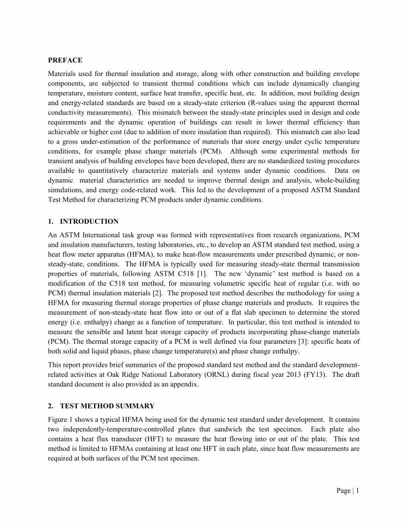
Figure 1 shows a typical HFMA being used for the dynamic test standard under development. It contains

two independently-temperature-controlled plates that sandwich the test specimen. Each plate also

contains a heat flux transducer (HFT) to measure the heat flowing into or out of the plate. This test

method is limited to HFMAs containing at least one HFT in each plate, since heat flow measurements are

required at both surfaces of the PCM test specimen.

Page | 2

A series of measurements are needed to determine the enthalpy

storage of a test specimen over a temperature range. First, both

HFMA plates are held at the same constant temperature until steady

state is achieved. Steady state is defined by the reduction in the

amount of energy entering the specimen from both plates, or vice-

versa, to a very small and nearly constant value. Next, both plate

temperatures are changed by identical amounts and held at the new

temperature until steady state is again achieved. The enthalpy

absorbed or released by the specimen from the time of the

temperature change until steady state is reached at the new plate

temperatures is recorded. Using a series of temperature step

changes of 1.5 ± 0.5°C, the cumulative enthalpy stored or released

over a certain temperature range is determined. The specific heats

of the solid and liquid phases are determined from the slope of the

sensible enthalpy storage as a function of temperature, above and

below the phase change temperature range. The proposed test

method requires the measurement temperature range to begin at

least 10°C below the phase change temperature range and continue

till 10°C above. Since the phase change temperatures may not be

known a priori, preliminary tests with coarser temperature step changes are useful in estimating the

required measurement temperature range. Complete details of the test method can be found in the draft

standard test method document (attached as Appendix A).

3. MEASURED PCM CHARACTERISTICS

In this section, some sample data are shown to illustrate the measurement of the different PCM

characteristics. It is important to note that these tests were done to assist in the development of the

standard test method, and the data shown here are not meant to formally characterize the PCM. Figure

2 and Figure 3 illustrate the determination of the phase change temperature range and the specific heats of

the solid and liquid phases. The melting and freezing threshold temperatures are determined by

performing linear regression using the enthalpy vs. temperature data points from the lowest and highest

temperatures, respectively.

To determine the threshold temperature for freezing, a linear regression is initially performed starting

with the two highest-temperature data points, resulting in a correlation coefficient of 1. This is followed

by a sequence of linear regressions in which the next lower temperature data point is added for each

successive calculation, until the correlation coefficient falls below 0.995. The temperature below which

the correlation coefficient falls below 0.995 is defined as the freezing threshold temperature. The slope of

line from the highest temperature to the freezing threshold is the specific heat of the PCM in its liquid

phase.

Prior experience has shown that, unlike freezing, there is no sharp transition at the beginning of melting

of PCMs and the correlation coefficient criterion of 0.995 to define melting onset is not appropriate.

Similar to freezing, the process starts with the two lowest-temperature data points (correlation coefficient

of 1) and progressively adds the next higher temperature data point until the linear regression calculation

returns a correlation coefficient less than 0.995. The last linear regression returning a correlation

Figure 1. Heat flow meter

apparatus (HFMA) for dynamic

of PCM. testing

Page | 3

coefficient greater than 0.995 defines a straight line that is used as a baseline for determining the

threshold temperature for melting. The melting threshold temperature is then defined as the temperature

above which the measured enthalpy deviates by a 20% or more from the calculated baseline. These

threshold criteria are based on the cumulative experience of the ASTM task group members in testing

PCMs.

Figure 2. Determination of melting threshold and specific heat of the liquid PCM.

Figure 3. Determination of freezing threshold and specific heat of the solid PCM.

Figure 2 and Figure 3 show the measured enthalpy storage of a sample PCM as a function of temperature

during freezing and melting. Based on the above criteria, the phase change range of the tested PCM was

18-26°C. The specific heats of the solid and liquid phases are determined from the slope of the enthalpy

vs. temperature curve, above and below the phase change range. Based on the data presented, the

volumetric specific heats of the solid and liquid PCM were 1.5 MJ/m3-K and 1.1 MJ/m

3-K.

The total enthalpy change between melting threshold (or lower limit of the phase change temperature

range, TL) and freezing threshold (upper limit, TU) includes both sensible and latent heat effects. The

difference between the measured total enthalpy change (∆h) and sensible enthalpy storage is defined as

the latent heat (hfs) and can be calculated as:

)()()( MeanUpMLMeanpF

T

T

fs TTcTTchhU

L

−−−−∆=∑ (1)

Page | 4

In eq. 1, ‘cpF’ and ‘cpM’ are the specific heats of the solid and liquid phases of the PCM and ‘Tmean’ is the

mid-point of the phase change temperature range. The calculated volumetric latent heat of the sample

PCM, based on above data, was 16.5 MJ/m3.

4. FY13 ORNL ACTIVITIES

During FY13, ORNL researchers led task group meetings at the October 2012 and April 2013 ASTM

committee meetings, to discuss the outstanding technical and editorial issues. In addition, there were

multiple online task group meetings. The draft standard was updated based on the outcomes of the

aforementioned meetings and submitted for balloting. In addition, testing of different PCM samples

continued to further add to the draft standard document. Part of the ORNL FY13 funds were used to

create a subcontract for Fraunhofer Center for Sustainable Energy, for further PCM testing and assisting

ORNL in resolving the negative votes and comments arising from the ASTM ballot process.

The draft standard was submitted to two ASTM ballots. The first ballot was at the sub-committee level,

in February 2013. Based on the comments received from this sub-committee ballot and those from the

subsequent meetings, the updated draft standard was submitted to the main committee ballot of

Committee C16 on Thermal Insulation in June 2013. The main committee ballot returned 26 affirmative

and 1 negative votes. The single negative vote is to be discussed and resolved in the upcoming October

2013 ASTM committee meeting.

5. FUTURE WORK

A teleconference was held with ASTM staff during August 2013, to discuss future activities and setting

up an inter-laboratory study (ILS). The next step is a repeatability test involving at least five tests each of

two most commonly-used types of PCMs. A full ILS will involve at least six testing laboratories and

cover the full scope of the standard. The ILS is required for a robust repeatability and reproducibility test

of the proposed standard test method.

6. REFERENCES

1. ASTM C518-10. Standard Test Method for Steady-State Thermal Transmission Properties by

Means of the Heat Flow Meter Apparatus. ASTM International, West Conshohocken, PA, United

States.

2. Tleoubaev, A. Brzezinski, A. and Braga, L. Accurate Simultaneous Measurements of Thermal

Conductivity and Specific Heat of Rubber, Elastomers, and Other Materials. 12th Brazilian

Rubber Technology Congress, 2008.

3. Gunther, E., Hiebler, S., Mehling, H. and Redlich, R., 2009. Enthalpy of Phase Change Materials

as a Function of Temperature: Required Accuracy and Suitable Measurement Methods.

International Journal of Thermophysics, Vol. 30, 2009, pp. 625 1257-1269.

Page | i

APPENDIX A

Standard Test Method for Using a Heat Flow Meter Apparatus

for Measuring Thermal Storage Properties of Phase Change

Materials and Products

1

This standard is issued under the fixed designation X XXXX; the number immediately following the designation indicates the year of original adoption or, in the case of revision, the year of last revision. A number in parentheses

indicates the year of last reapproval. A superscript epsilon (ε) indicates an editorial change since the last revision or

reapproval.

1. Scope

1.1 This test method covers the measurement of non-steady-state heat flow into or out of a flat

slab specimen to determine the stored energy (i.e. enthalpy) change as a function of

temperature using a heat flow meter apparatus (HFMA).

1.2 In particular, this test method is intended to measure the sensible and latent heat storage

capacity for products incorporating phase-change materials (PCM). The storage capacity of

a PCM is well defined via four parameters: specific heats of both solid and liquid phases,

phase change temperature(s) and phase change enthalpy (1).

1.3 To more accurately predict thermal performance, information about the performance of PCM

products under dynamic conditions is needed to supplement the properties (thermal

conductivity) measured under steady-state conditions.

Note 1: This test method defines a dynamic test protocol for products or composites containing PCMs. Due to the

macroscopic structure of these products or composites, small sample sizes used in conventional Differential Scanning

Calorimeter (DSC) measurements, as specified in E793 and E967, are not representative of the relationship between

temperature and enthalpy storage of full-scale PCM products.

1.4 This test method is based upon the HFMA technology used for Test Method C518 but

includes modifications for specific heat and enthalpy change measurements for PCM

products as outlined in this test method.

1.5 Heat flow measurements are required at both the top and bottom HFMA plates for this test

method. Therefore, this test method applies only to HFMAs that are equipped with at least

one heat flux transducer on each of the two plates and that have the capability for

computerized data acquisition and temperature control systems. Further, the amount of

energy flowing through the transducers must be measureable at all points in time. Therefore,

the transducer output shall never be saturated during a test.

1.6 This test method makes a series of measurements to determine the enthalpy storage of a test

specimen over a temperature range. First, both HFMA plates are held at the same constant

temperature until steady state is achieved. Steady state is defined by the reduction in the

amount of energy entering the specimen from both plates to a very small and nearly constant

1 This Practice/Guide is under the jurisdiction of ASTM Committee C16 and is the direct responsibility of

Subcommittee C16.30.

Current edition approved XXX. XX, XXXX. Published XX XXXX. DOI: 10.1520/XXXXX-XX.

Page | ii

value. Next, both plate temperatures are changed by identical amounts and held at the new

temperature until steady state is again achieved. The enthalpy absorbed or released by the

specimen from the time of the temperature change until steady state is again achieved will be

recorded. Using a series of temperature step changes, the cumulative enthalpy stored or

released over a certain temperature range is determined.

1.6.1 The specific heats of the solid and liquid phases are determined from the slope of the

sensible enthalpy storage as a function of temperature, above and below the phase change

temperature range.

1.7 Calibration of the HFMA to determine the ‘correction factors’ for the enthalpy stored within

the plate heat flux transducers and any material placed between the test specimen and the

HFMA plates must be performed following Annex A. These correction factors are functions

of the beginning and ending temperatures for each step, as described in Annex A.

1.8 This test method applies to PCMs and composites, products and systems incorporating

PCMs, including: dispersed in, or combined with, a thermal insulation material, boards or

membranes containing concentrated or dispersed PCM, etc. Specific examples include solid

PCM composites and products, loose blended materials incorporating PCMs, and discretely

contained PCM.

1.9 This test method may be used to characterize material properties, which may or may not be

representative of actual conditions of use.

1.10 The values stated in SI units are to be regarded as standard. No other units of

measurement are included in this standard.

1.11 This standard does not purport to address all of the safety concerns, if any, associated

with its use. It is the responsibility of the user of this standard to establish appropriate safety

and health practices and determine the applicability of regulatory limitations prior to use.

2. Referenced Documents

2.1 ASTM Standards:

C168 Terminology Relating to Thermal Insulation

C518 Standard Test Method for Steady-State Thermal Transmission Properties by Means of the Heat

Flow Meter Apparatus

E793 Standard Test Method for Enthalpies of Fusion and Crystallization by DSC

E967 Standard Test Method for Temperature Calibration of Differential Scanning Calorimeters and

Differential Thermal Analyzers

2.2 Other Standard:

RAL-GZ 896 Phase Change Material, German Institute for Quality Assurance and Certification

E.V.2.

2 Available online at http://www.pcm-ral.de/uploads/media/RAL_GZ_896_Phase_Change_Material_2010_01.pdf

Page | iii

3. Terminology

3.1 Definitions—Terminology C168 applies to terms used in this specification

3.2 Definitions of Terms Specific to This Standard:

3.2.1 phase change material (PCM), n—a material that changes it physical state (solid to

liquid or vice-versa) over a certain temperature range, used in engineering applications

specifically to take advantage of its latent heat storage properties

3.2.2 PCM Active Range, n—a broad temperature range in which a PCM changes phase from

solid to liquid (melting) or liquid to solid (freezing), with associated enthalpy changes

3.2.3 PCM composite, n–material embedded with PCM to enhance its thermal performance

3.2.4 PCM product, n–material amended to include enthalpy storage capabilities via

inclusion of PCM or PCM composites

3.2.5 PCM system, n-array or assembly of PCM products

3.3 Symbols and Units—The symbols used in this test method have the following

significance:

3.3.1 A—HFMA metering area, m2.

3.3.2 Chft(Tbegin,Tend)—Correction factor for heat storage in the heat flux transducers, J/(m2-

ºC)

3.3.3 Cother(Tbegin,Tend)—Correction factor for heat storage in other materials used to surround

the test specimen, J/(m2-ºC)

3.3.4 cp(T)-specific heat as a function of temperature, J/kg-ºC.

3.3.5 cpM – specific heat of a melted PCM product, defined at a temperature greater than the

upper limit of the PCM Active Range, J/kg-ºC.

3.3.6 cpM,A – areal specific heat of a melted PCM product, defined at a temperature greater

than the upper limit of the PCM Active Range, J/m2-ºC.

3.3.7 cpM,V – volumetric specific heat of a melted PCM product, defined at a temperature

greater than the upper limit of the PCM Active Range, J/m3-ºC.

3.3.8 cpF – specific heat of a frozen PCM product, defined at a temperature less than the

lower limit of the PCM Active Range, J/kg-ºC.

3.3.9 cpF,A – areal specific heat of a frozen PCM product, defined at a temperature less than

the lower limit of the PCM Active Range, J/m2-ºC.

3.3.10 cpF,V – volumetric specific heat of a frozen PCM product, defined at a temperature less

than the lower limit of the PCM Active Range, J/m3-ºC.

3.3.11 E—heat flux transducer output, µV

3.3.12 f—fraction of total PCM mass in the sample that has undergone phase change,

dimensionless

3.3.13 h — enthalpy, J/kg

3.3.14 hA—areal enthalpy, J/m2

Page | iv

3.3.15 hfs—latent heat per unit mass, J/kg

3.3.16 hfs,A—latent heat per unit area, J/m2

3.3.17 hV—volumetric enthalpy, J/m3

3.3.18 k-thermal conductivity, W/m-K.

3.3.19 L—thickness of the test specimen, usually equal to the separation between the hot and

cold plate assemblies during testing, m.

3.3.20 N—number of heat flux readings at a specific temperature step

3.3.21 q—heat flux (heat flow rate, Q, through area A), W/m2.

3.3.22 qequilibrium—average heat flux at the end of a specific temperature step, W/m2.

3.3.23 Q—heat flow rate in the metered area, W.

3.3.24 R—thermal resistance, (m2·K)/W.

3.3.25 S—calibration factor of the heat flux transducer, (W/m2)/V.

3.3.26 T – Temperature, °C.

3.3.27 Tbegin—Beginning temperature for each temperature step, °C.

3.3.28 Tend— Ending temperature for each temperature step, °C.

3.3.29 TL—lower temperature limit of the PCM Active Range, °C.

3.3.30 TU—upper temperature limit of the PCM Active Range, °C.

3.3.31 ∆T—temperature difference during a temperature step (Tend - Tbegin), °C.

3.3.32 α — thermal diffusivity, m2/s.

3.3.33 ρ—(bulk) density of the material tested, kg/m3.

3.3.34 λ—thermal conductivity, W/(m·K).

3.3.35 τ—time interval, s.

3.3.36 ∆τ—time interval corresponding to each individual flux reading (data value), s.

3.4 Subscripts and Superscripts—

3.4.1 A – Areal, per m2

3.4.2 F – Frozen, solid

3.4.3 fs – latent, associated with the transition from solid to liquid or liquid to solid

3.4.4 i,k – index denoting ith

, kth

member of a series

3.4.5 L – Lower

3.4.6 M – Melted, liquid

3.4.7 U - Upper

3.4.8 V – Volumetric, per m3

Page | v

4. Summary of the Test Method

4.1 This test method describes a method of using a heat flow meter apparatus (HFMA) to

perform heat flux measurements on samples exposed to dynamic, that is non-steady-state,

temperature conditions. The HFMA plates are allowed to stabilize at a certain identical

temperature, above or below the PCM Active Range, and then their temperatures are

incrementally decreased or increased. The plates are allowed to reach steady-state after each

temperature step and the enthalpy change of the test specimen is determined for each step change

in temperature, hence the dynamic nature of the test.

Note 2: Since the ‘dynamic’ portion of the test method does not involve measurements made under steady-state

conditions, nor lead to determination of steady-state thermal transmission properties, the Test Method C518 cannot be

used.

4.1.1 The test method is specifically designed to address materials and products that undergo

physical changes with latent heat absorption or release during the course of the test. In

particular, a phase transition will occur within PCM products, when the test temperatures span

the PCM Active Range.

4.2 The object of the test, especially for a PCM product, is generally to determine the

temperature dependence of the enthalpy storage characteristics of the specimen.

5. Significance and Use

5.1 Materials used in building envelopes to enhance energy efficiency, including PCM

products used for thermal insulation, thermal control, and thermal storage, are subjected to

transient thermal environments, including transient or cyclic boundary temperature conditions.

This test method is intended to enable meaningful PCM product classification, as steady-state

thermal conductivity alone is not sufficient to characterize PCMs.

Note 3: This test method defines a dynamic test protocol for complex products or composites containing PCMs. Due to

the macroscopic structure of these products or composites, conventional measurements using a Differential Scanning

Calorimeter (DSC) as specified in E793 and E967, which use very small samples, are not representative of the relationship

between temperature and enthalpy storage of full-scale PCM products due to the sample size limitation.

5.2 Dynamic measurements of the thermal performance of PCM products shall only be

performed by qualified personnel with understanding of heat transfer and error propagation.

Familiarity with the configuration of both the apparatus and the product is necessary.

5.3 This test method focuses on testing PCM products used in engineering applications,

including in building envelopes to enhance the thermal performance of insulation systems.

5.3.1 Applications of PCM in building envelopes take multiple forms, including: dispersed

in, or otherwise combined with, a thermal insulation material; a separate object implemented in

the building envelope as boards or membranes containing concentrated PCM that operates in

conjunction with a thermal insulation material. Both of these forms enhance the performance of

the structure when exposed to dynamic, i.e., fluctuating, boundary temperature conditions.

5.3.2 PCMs can be studied in a variety of forms: as the original “pure” PCM; as a composite

containing PCM and other embedded materials to enhance thermal performance; as a product

containing PCM or composite (such as micro- or macro-encapsulated PCM); or as a system,

comprising arrays or assemblies of PCM products.

Page | vi

5.4 This test method describes a method of using a heat flow meter apparatus to determine

key properties of PCM products, which are listed below. Engineers, architects, modelers, and

others require these properties to accurately predict the in-situ performance of the products (2).

5.5 The objective is generally to conduct a test under temperature conditions that will induce

a phase transition—e.g., melting or freezing—in the PCM product during the course of the test.

5.6 Determination of thermal storage properties is the objective of this test method, and key

properties of interest include the following:

5.6.1 PCM Active Range, that is temperatures over which the phase transitions occur, for

both melting and freezing of the PCM product or composites containing PCMs

5.6.2 Specific heat of the fully melted and fully frozen product, defined outside the PCM

Active Range

5.6.3 Enthalpy change as a function of temperature, h(T), including both sensible and latent

components

5.6.4 Enthalpy plot—a histogram or table that indicates the change in enthalpy associated

with incremental temperature changes that span the tested temperature range

5.6.5 Enthalpy of phase transition during the PCM melting and freezing processes in

materials and composites containing PCMs

5.7 PCM products often possess characteristics that complicate measurement and analysis of

phase transitions during a test. Following are some of the known issues with PCMs:

5.7.1 Imprecise PCM Active Range —PCMs in general do not have precise melting or

freezing temperatures, and the entire active temperature range, from the beginning to the end of

phase transitions, must be determined.

Note 4: The onset of freezing will not necessarily coincide with the end of melting. Therefore, the freeze and melt enthalpy

curves must be independently defined to determine the PCM Active Range.

5.7.2 Multiple phase transitions—many PCMs exhibit a solid-solid transition with

significant latent heat effects at temperatures near the melting transition

5.7.3 Sub-cooling—occurs when the specimen cools below its nominal freezing temperature

before it actually begins to freeze, thus exhibiting an unusual enthalpy-temperature curve. The

temperatures to initiate solid-liquid and solid-solid phase changes are often dependent on heating

and cooling rate, purity of the PCM and if the PCM is somewhat amorphous (non-crystalline).

5.7.4 Hysteresis—occurs when a specimen heated from one temperature to another, and then

returned to the original temperature, absorbs more (or less) heat at any particular temperature

during the heating stage than it releases during cooling.

5.8 The properties measured are determined by fundamental thermophysical properties of the

constituent materials of the product, and are thus inherent to the PCM product. The desired

thermal performance enhancement, however, will depend strongly on the particular environment,

climate, and mode of the actual engineering application of the PCM.

6. Apparatus

Page | vii

6.1 Follow the Apparatus section of Test Method C518 with these additional requirements:

6.1.1 A minimum of two heat flux transducers, one mounted on each plate of the apparatus,

are required.

6.1.2 The ability to scan temperature and heat flux data at specified intervals and store

results in a form that is immediately accessible in real time to the user or other programs running

concurrently is required; e.g., a text file to which data are written after each scan. The ability to

record a time stamp of each scan is required.

6.1.3 The ability to accept a user-defined temperature program for control of both plate

temperatures. This test method includes a series of temperature steps, with specified intervals

determined by time or equilibrium criteria.

Note 5: Independent time or equilibrium criteria control for each setpoint will facilitate the test.

6.1.4 The amount of energy flowing through the transducers must be measureable at all

times. To avoid saturating the transducers, either their voltage gain must be variable, or in

apparatus without variable transducer gain, the alternative approaches described in Appendix D

must be followed.

7. Specimen Preparation

7.1 Instructions are given here separately for solid samples, loose blended materials, and

discretely contained PCM.

7.2 For solid samples such as gypsum wallboard containing PCM (3-5).

7.2.1 Cut the specimen to the same size as the HFMA plate area.

Note 6: If the specimen has a conductive facing, e.g., foil, place a sheet of craft paper between the facing and the

corresponding apparatus plate. If the heat capacity of this sheet is expected to be significant relative to the enthalpy

storage of the specimen, independently measure the heat capacity in the same manner as for the HFMA transducers,

described in Annex A. Then correct the measured heat flow into the assembly for this material as described in Section 10.

7.3 For loose material blended with PCM (6,7).

7.3.1 Construct the sides of a frame using thin low mass material between 2.5 to 5 cm in

height and sized so the frame will be located at the periphery of the test chamber. Affix a net

material to form the frame bottom.

7.3.2 Since the frame is located far from the metering area, it is unlikely that the frame

presence will have a significant effect on the thermal measurement. This shall be verified by

separate measurement on solid specimens made with and without the sample frame.

7.4 For arrays of PCM pouches or PCM containers (8).

7.4.1 Ensure the portion of the product within the metered area is representative of the array

pattern.

7.4.2 A sketch or photograph of the test specimen is required for this type of product, due to

the spatial non-uniformities and discontinuities that are common with this product type.

7.5 Ensure good contact between the HFMA plates and the product. If necessary, use an

elastomeric or soft foam rubber sheet between one or both sides of the product and the

Page | viii

corresponding apparatus plate. This sheet will improve contact between the controlled

temperature plates and prevent air circulation between the panel and the plates. The enthalpy

storage correction for the sheet(s) must be independently measured, in the same manner as for

the HFMA transducers, as described in Annex A. The measured heat flow into the assembly

must then be corrected for this material as described in Section 10.3.

7.6 For PCM products with high lateral thermal conductivity, use an insulating frame to

avoid significant edge losses. Ensure the frame is far away from the metered area to maximize

the one-dimensional heat flow in the metered area.

8. Calibration

8.1 Prior to using this test method, calibrate the HFMA to determine the temperature-

dependent calibration coefficients for both heat flux transducers using the procedure for the

multiple temperature and thickness points in the Calibration section of Test Method C518.

8.2 The heat flux levels obtained during an HFMA test run are, in general, determined by

heat flowing into or out of the specimen. The heat flux readings are also impacted by the heat

that enters or leaves the transducers themselves, as a result of the change of the transducer

temperature that corresponds to the change in plate temperature. Such heat flow is incidental to

the values used in characterizing the PCM product. Therefore, separately calibrate the heat flux

transducers within the HFMA to measure the correction factor for heat storage in the heat flux

transducers. This additional apparatus calibration is described in Annex A.

9. Procedure

9.1 Personnel qualifications: This test method shall only be performed by qualified personnel

with experience in heat transfer analysis and experimental error propagation. To ensure accurate

measurement, the operator shall be fully proficient in the operation of the equipment and must

have detailed familiarity with the configuration of the apparatus, the apparatus control and data

reporting software, and the specimen itself.

9.2 Procedure overview: In order to characterize the PCM product, test parameter definitions

are required, as are multiple series of measurements at discrete temperature steps. Instructions

are given here to first define the general process used during a series of measurements (9.3);

describe how to determine the test parameters (9.4); and finally, to apply this process to

characterize the PCM product (9.5). Additional instructions are included to describe an optional

investigation of the hysteresis within partially melted or frozen specimens (9.6, Appendix E).

9.3 Define general series of temperature steps for both plates, e.g. 11ºC and 11ºC, 13ºC and

13ºC, 15ºC and 15ºC, and so on.

9.3.1 To measure the enthalpy stored in the test specimen in each temperature range, make a

series of measurements.

9.3.2 First, both plates shall be held at the same constant temperature until steady state is

achieved.

Note 7: Please see Annex A for a description of experimental work that has been done with an apparatus with plates at

different temperatures to achieve the same goals.

Page | ix

9.3.2.1 Steady state is defined by the reduction in the amount of energy entering the

specimen from both plates to a very small and nearly constant value. See section 10.2.

9.3.3 After steady state is achieved, both plate temperatures will be changed to the same new

temperature and held at that value until steady state is again achieved.

9.3.4 The cumulative amount of energy that enters the specimen from the time of the

temperature change until steady state is again achieved will be recorded.

9.3.5 Heat flux readings shall include the proper sign to indicate direction of heat flow;

normally a positive reading indicates heat entering sample, and negative values indicate heat

leaving the specimen.

9.3.6 The initial temperature selection, the temperature difference between setpoints, and the

number of temperature steps, will vary according to the purpose of each particular test series.

Note 8: The temperature range available depends on the construction of the HFMA equipment, the heat rejection bath

temperature, and the calibration of the equipment.

9.4 Determine the test parameters.

9.4.1 An initial test shall be used to estimate the PCM Active Range and determine the time

required for each temperature step. This step is not required if the specimen phase change

characteristics are already well known, for example from differential thermal analysis (DTA)

tests or differential scanning calorimetry (DSC) tests (using the step method or appropriately

slow heating and cooling rates, as described in Ref. 9).

9.4.2 Make series of measurements, as described in 9.3, starting at a temperature at least

10ºC below the expected melting temperature, or at the lowest temperature available on the

HFMA, whichever is higher. Use temperature difference steps of 1.5±0.5ºC. Allow a minimum

of two hours for each setpoint during the initial specimen characterization.

9.4.3 End the series when the amount of energy stored in a temperature step returns to a

small value, that is, when the test specimen is fully melted. See section 10.2.

Note 9: As described in Section 10.2, the amount of time required at each temperature step will vary depending on the

size of the temperature step, the thermal diffusivity of the specimen, and the amount of enthalpy storage that occurs over

that temperature step.

9.4.4 Repeat this procedure starting at the fully melted temperature condition and decreasing

the plate temperatures in 1.5±0.5ºC steps until the amount of energy stored in a temperature step

returns to a small value, that is, when the test specimen is fully frozen. See section 10.2.

9.4.5 Examine the data as described in section 10. Determine the estimated PCM Active

Range, the desired temperature step size, and the amount of time required for each step.

9.4.6 An example of such a test series is shown in Annex B.

9.5 Characterize the PCM product.

9.5.1 Make a series of measurements, as described in 9.3, starting at a temperature at least

10ºC below estimated PCM Active Range, and heating the plates with temperature difference

steps of 1.5±0.5ºC. End at a temperature at least 10ºC above the estimated PCM Active Range.

The amount of time required at each temperature step shall be as determined in 10.2.

Note 10: The minimum and maximum temperature difference step size will be limited by the combined uncertainty of the

temperature measurement and heat flux measurement within the HFMA.

Page | x

9.5.2 Make a series of measurements, as described in 9.3, starting at a temperature at least

10ºC above the estimated PCM Active Range, and cooling the plates with temperature difference

steps of 1.5±0.5ºC. End at a temperature at least 10ºC below the estimated PCM Active Range.

9.5.3 Examine the data as described in Section 10 to determine:

9.5.3.1 Whether either of the data series shall be repeated using longer equilibrium times at

any particular temperature.

9.5.3.2 Whether the temperature range needs to be expanded to capture the full PCM Active

Range.

9.5.4 A minimum of three heating series, as described in Section 9.5.1, and a minimum of

three cooling series, as described in Section 9.5.2, are required.

9.5.4.1 In order to define the enthalpy curve of enthalpy storage vs. temperature with

adequate precision, select beginning temperatures for the subsequent heating and cooling series

that differ from those used for the initial heating and cooling series.

Note 11: For example: If the initial heating series spanned 10 to 30ºC in 2ºC steps, retain the 2ºC step size, but start the

second heating series at 10.6ºC and the third heating series at 11.3ºC. If the initial cooling series spanned 30 to 10ºC in 2ºC

steps, retain the 2ºC step size, but start the second heating series at 29.4ºC and the third heating series at 28.7ºC.

9.5.4.2 Examine the data as described in Section 10.2 to determine whether either of the data

series shall be repeated using longer equilibrium times at any particular temperature.

9.6 Hysteresis effects when starting from partially frozen or partially melted material may be

explored using the method described in Appendix E.

10. Calculations

10.1 Calculations Overview: The calculations require several separate stages. First it is

necessary to examine the data to evaluate whether an adequate amount of time was spent at each

and every temperature step (10.2). Once this has been established, it is possible to calculate the

net enthalpy storage within the test specimen corresponding to each temperature step (10.3). That

data form can then be used to express the enthalpy of the product as a function of temperature

(10.4); to define the specific heat of the fully melted and fully frozen product (10.5, 10.6); and to

define the latent heat of the product (10.7).

10.2 Evaluate adequacy of time intervals at each temperature step

10.2.1 The amount of time required at each temperature step will vary depending on the size

of the temperature step, the thermal diffusivity of the specimen, the material thickness, and the

amount of enthalpy storage that occurs over that temperature step. The time interval required to

reach steady state during phase change phenomena are much greater than time intervals required

when the material is subjected to sensible enthalpy storage phenomena.

10.2.1.1 The maximum heat rate into or out of the specimen is limited by apparatus

capability and the specimen thermal diffusivity. It is possible to estimate the minimum amount of

time (τmin,est) needed for each step by neglecting the apparatus limits and the impact of thermal

storage on the thermal transmittance through the specimen, as shown in Eq. 1. This approach is

only possible when there is some basis for estimating the enthalpy storage needed for that

particular temperature step and when an estimate is available for the thermal conductivity of the

Page | xi

material. Possible sources for the enthalpy storage estimate include prior heating or cooling

series or data from a DSC run.

����,��� �����������������������������������������������������������������������������������������

or, ����,��� �������∆�!"∆� �� #⁄ �% &

�������'#" (1)

Note 12: If data are available to permit the calculation shown in Eq. 1, reasonable rules of thumb for the adequate total

time for that temperature step would be: (1) for heating away from the expected latent range, use 1.5 times the estimated

minimum; (2) for heating within the latent range, use 2.5 times the estimated minimum; (3) for cooling away from the

expected latent range, use 2.5 times the estimated minimum; (4) for cooling within the latent range, use 5 times the

estimated minimum.

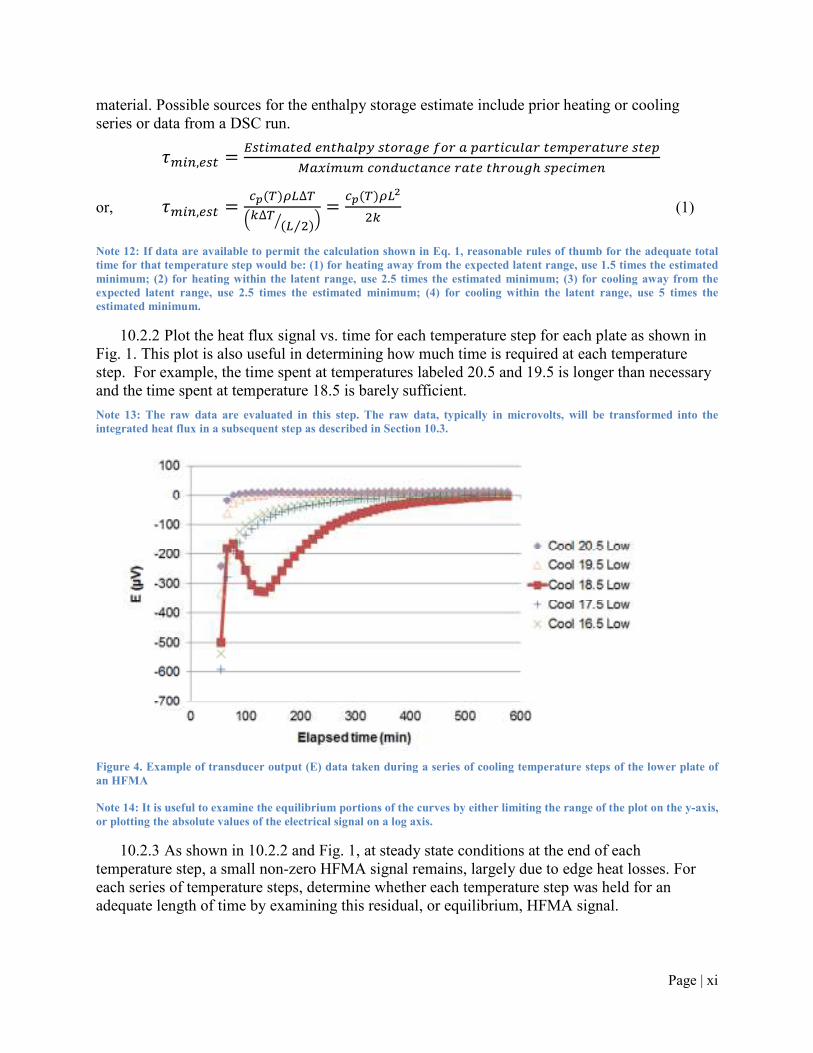
10.2.2 Plot the heat flux signal vs. time for each temperature step for each plate as shown in

Fig. 1. This plot is also useful in determining how much time is required at each temperature

step. For example, the time spent at temperatures labeled 20.5 and 19.5 is longer than necessary

and the time spent at temperature 18.5 is barely sufficient.

Note 13: The raw data are evaluated in this step. The raw data, typically in microvolts, will be transformed into the

integrated heat flux in a subsequent step as described in Section 10.3.

Figure 4. Example of transducer output (E) data taken during a series of cooling temperature steps of the lower plate of

an HFMA

Note 14: It is useful to examine the equilibrium portions of the curves by either limiting the range of the plot on the y-axis,

or plotting the absolute values of the electrical signal on a log axis.

10.2.3 As shown in 10.2.2 and Fig. 1, at steady state conditions at the end of each

temperature step, a small non-zero HFMA signal remains, largely due to edge heat losses. For

each series of temperature steps, determine whether each temperature step was held for an

adequate length of time by examining this residual, or equilibrium, HFMA signal.

Page | xii

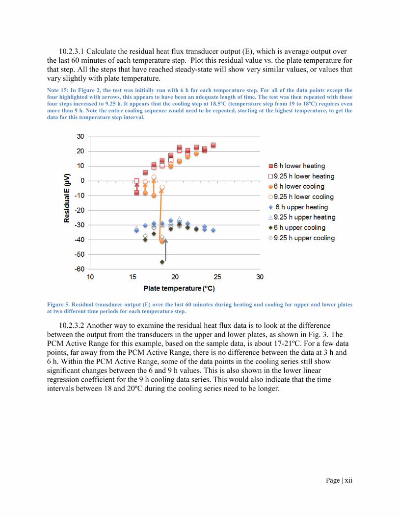
10.2.3.1 Calculate the residual heat flux transducer output (E), which is average output over

the last 60 minutes of each temperature step. Plot this residual value vs. the plate temperature for

that step. All the steps that have reached steady-state will show very similar values, or values that

vary slightly with plate temperature.

Note 15: In Figure 2, the test was initially run with 6 h for each temperature step. For all of the data points except the

four highlighted with arrows, this appears to have been an adequate length of time. The test was then repeated with those

four steps increased to 9.25 h. It appears that the cooling step at 18.5ºC (temperature step from 19 to 18ºC) requires even

more than 9 h. Note the entire cooling sequence would need to be repeated, starting at the highest temperature, to get the

data for this temperature step interval.

Figure 5. Residual transducer output (E) over the last 60 minutes during heating and cooling for upper and lower plates

at two different time periods for each temperature step.

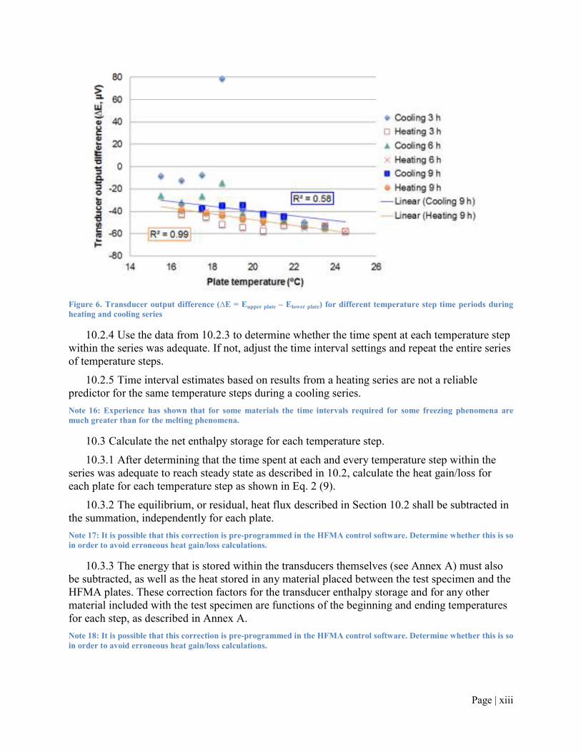
10.2.3.2 Another way to examine the residual heat flux data is to look at the difference

between the output from the transducers in the upper and lower plates, as shown in Fig. 3. The

PCM Active Range for this example, based on the sample data, is about 17-21ºC. For a few data

points, far away from the PCM Active Range, there is no difference between the data at 3 h and

6 h. Within the PCM Active Range, some of the data points in the cooling series still show

significant changes between the 6 and 9 h values. This is also shown in the lower linear

regression coefficient for the 9 h cooling data series. This would also indicate that the time

intervals between 18 and 20ºC during the cooling series need to be longer.

Page | xiii

Figure 6. Transducer output difference (∆E = Eupper plate – Elower plate) for different temperature step time periods during

heating and cooling series

10.2.4 Use the data from 10.2.3 to determine whether the time spent at each temperature step

within the series was adequate. If not, adjust the time interval settings and repeat the entire series

of temperature steps.

10.2.5 Time interval estimates based on results from a heating series are not a reliable

predictor for the same temperature steps during a cooling series.

Note 16: Experience has shown that for some materials the time intervals required for some freezing phenomena are

much greater than for the melting phenomena.

10.3 Calculate the net enthalpy storage for each temperature step.

10.3.1 After determining that the time spent at each and every temperature step within the

series was adequate to reach steady state as described in 10.2, calculate the heat gain/loss for

each plate for each temperature step as shown in Eq. 2 (9).

10.3.2 The equilibrium, or residual, heat flux described in Section 10.2 shall be subtracted in

the summation, independently for each plate.

Note 17: It is possible that this correction is pre-programmed in the HFMA control software. Determine whether this is so

in order to avoid erroneous heat gain/loss calculations.

10.3.3 The energy that is stored within the transducers themselves (see Annex A) must also

be subtracted, as well as the heat stored in any material placed between the test specimen and the

HFMA plates. These correction factors for the transducer enthalpy storage and for any other

material included with the test specimen are functions of the beginning and ending temperatures

for each step, as described in Annex A.

Note 18: It is possible that this correction is pre-programmed in the HFMA control software. Determine whether this is so

in order to avoid erroneous heat gain/loss calculations.

Page | xiv

10.3.4 Eq. 2 shows the calculation of the enthalpy storage in the specimen for a given

temperature interval (Tbegin, Tend). The recorded heat flux for both plates, corrected for the

residual equilibrium heat flux, is multiplied by the length of time ( τ∆ ) for each data point ( iq ),

and summed over the total number of data points (N) for the given temperature interval ( T∆ ).

After subtracting the transducer heat storage correction factors, as well as the correction for any

other material included within the HFMA, from the sum of the heat flow into the specimen, the

total amount of enthalpy stored in the specimen during that temperature interval is calculated as

shown in Eq. 2.

( )

( ) ),(),(

),(),(

lower

endbeginendbeginhft

1

mequilibriui

upper

endbeginendbeginhft

1

mequilibriui

∆−∆−

∆−

+

∆−∆−

∆−=

∑

∑

=

=

TTTCTTTCqq

TTTCTTTCqqh

other

N

i

other

N

i

A

τ

τ

(2)

10.4 Combine the temperature step data to define the enthalpy storage as a function of

temperature

10.4.1 Define the zero amount of cumulative heat as corresponding to the bottom of the

step(s) starting from the lowest temperature used in 9.5.

10.4.2 Plot the corrected cumulative heat into or out of the specimen vs. the ending

temperature for each step. An example is shown in Annex B.

10.4.3 That plot of areal enthalpy (hA , J/m

2) can also be manipulated to show the specific

enthalpy (h, J/kg) and volumetric enthalpy (hV, J/m3)as a function of temperature. See Annex B

for an example of merging the data from multiple series onto a single plot of hV vs. T.

ℎ�)� ℎ*�)�/�,-� (3)

ℎ.�)� ℎ*�)�/- (4)

10.4.4 The data from heating series and cooling series shall be kept separate except that the

final enthalpy from the heating series shall be taken as the starting enthalpy for the cooling

series. See Annex B.

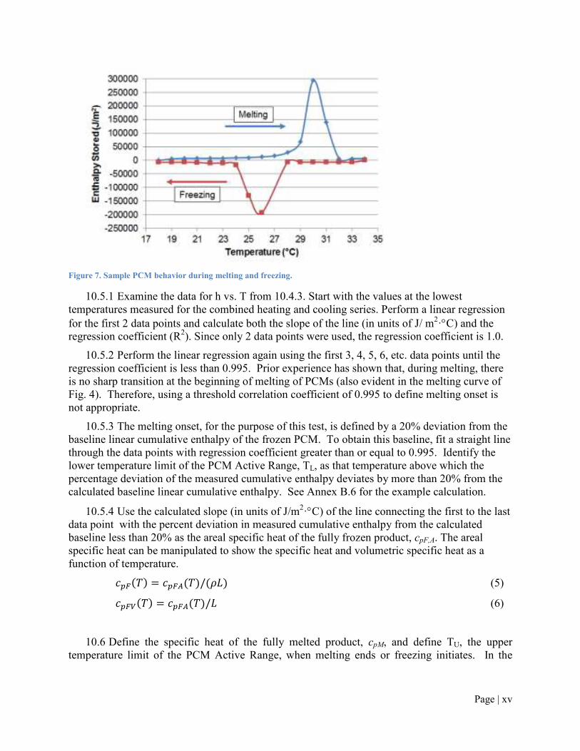
10.5 Define the specific heat of the fully frozen product, cpF, and define TL, the lower

temperature limit of the PCM Active Range, when the melting initiates or freezing ends. Fig. 4

shows a sample PCM behavior during melting and freezing. In this example, the freezing ends at

a lower temperature than the melting initiation, and TL needs to be defined based on the freezing

series. See Annex B.6 for an example calculation.

Note 19: The accuracy of TL will be limited by the temperature step size.

Page | xv

Figure 7. Sample PCM behavior during melting and freezing.

10.5.1 Examine the data for h vs. T from 10.4.3. Start with the values at the lowest

temperatures measured for the combined heating and cooling series. Perform a linear regression

for the first 2 data points and calculate both the slope of the line (in units of J/ m2·°C) and the

regression coefficient (R2). Since only 2 data points were used, the regression coefficient is 1.0.

10.5.2 Perform the linear regression again using the first 3, 4, 5, 6, etc. data points until the

regression coefficient is less than 0.995. Prior experience has shown that, during melting, there

is no sharp transition at the beginning of melting of PCMs (also evident in the melting curve of

Fig. 4). Therefore, using a threshold correlation coefficient of 0.995 to define melting onset is

not appropriate.

10.5.3 The melting onset, for the purpose of this test, is defined by a 20% deviation from the

baseline linear cumulative enthalpy of the frozen PCM. To obtain this baseline, fit a straight line

through the data points with regression coefficient greater than or equal to 0.995. Identify the

lower temperature limit of the PCM Active Range, TL, as that temperature above which the

percentage deviation of the measured cumulative enthalpy deviates by more than 20% from the

calculated baseline linear cumulative enthalpy. See Annex B.6 for the example calculation.

10.5.4 Use the calculated slope (in units of J/m2·°C) of the line connecting the first to the last

data point with the percent deviation in measured cumulative enthalpy from the calculated

baseline less than 20% as the areal specific heat of the fully frozen product, cpF,A. The areal

specific heat can be manipulated to show the specific heat and volumetric specific heat as a

function of temperature.

/�0�)� /�0*�)�/�,-� (5)

/�0.�)� /�0*�)�/- (6)

10.6 Define the specific heat of the fully melted product, cpM, and define TU, the upper

temperature limit of the PCM Active Range, when melting ends or freezing initiates. In the

Page | xvi

example shown in Fig. 4, the melting ends at a higher temperature and will define TU. See Annex

B.6 for an example calculation.

Note 20: The accuracy of TU will be limited by the temperature step size.

10.6.1 Examine the data for h vs. T from 10.4.3. Start with the values at the highest

temperatures measured for the combined heating and cooling series. Perform a linear regression

for the first 2 data points and calculate both the slope of the line (in units of J/kg·ºC) and the

regression coefficient (R2). Since only 2 data points were used, the regression coefficient is 1.0.

10.6.2 Perform the linear regression again using the first 3, 4, 5, 6, etc. data points until the

regression coefficient is less than 0.995. Identify the upper temperature limit of the PCM Active

Range, TU, as that temperature at which the regression coefficient first dropped below 0.995.

Based on prior experience, the enthalpy storage curve of the PCM exhibits a sharp transition at

the freezing onset. Therefore, TU is defined solely by the temperature below which the

correlation coefficient drops below 0.995.

10.6.3 Use the calculated slope of the line connecting the first to the last data point set with a

regression coefficient greater than 0.995 as the specific heat of the fully melted product, cpM.

10.7 Calculate the latent heat.

10.7.1 The total enthalpy change between TL and TU includes both sensible and latent heat

effects. Use the specific heat of the fully frozen product below the mean temperature of the

PCM Active Range, and the specific heat of the fully melted state above the mean temperature of

the PCM Active Range to define the sensible heat storage over the temperature range. The

difference between the total and sensible heat storage is the latent heat (hfs).

h fs = (∆h)TL

TU

∑ − cpF (TMean −TL )− cpM (TU −TMean ) = (∆h)TL

TU

∑ −(cpF + cpM )(TU −TL )

2

(7)

10.7.2 The areal form of the latent heat is shown in Eq. 8.

(8)

11. Report

11.1 For each test, report the following information:

11.1.1 Identify the report with a unique numbering system to allow traceability back to the

individual measurements taken during the test performed.

11.1.2 Identify the material and give a physical description.

11.1.2.1 Provide a specimen diagram or photograph if any materials other than the PCM

product were placed in the HFMA, or if the area of the specimen is different from the area of the

HFMA plates.

11.1.2.2 Provide a specimen diagram if the test specimen consisted of arrays of PCM

pouches or PCM containers

11.1.3 Provide a brief conditioning history of the specimen, if known.

h fs,A = h fs ×ρ × L

Page | xvii

11.1.4 Thickness of the specimen as received and as tested, m.

11.1.5 Mass of the specimen, kg.

11.1.6 Volume of the specimen, m3.

11.1.7 Density of the specimen, kg/m3.

11.1.8 Area of the specimen exposed to each HFMA plate, m2.

11.1.9 Method and environment used for conditioning, if used.

11.1.10 Dates the tests started and ended.

11.1.11 The temperature step size(s) used in the melting and freezing tests.

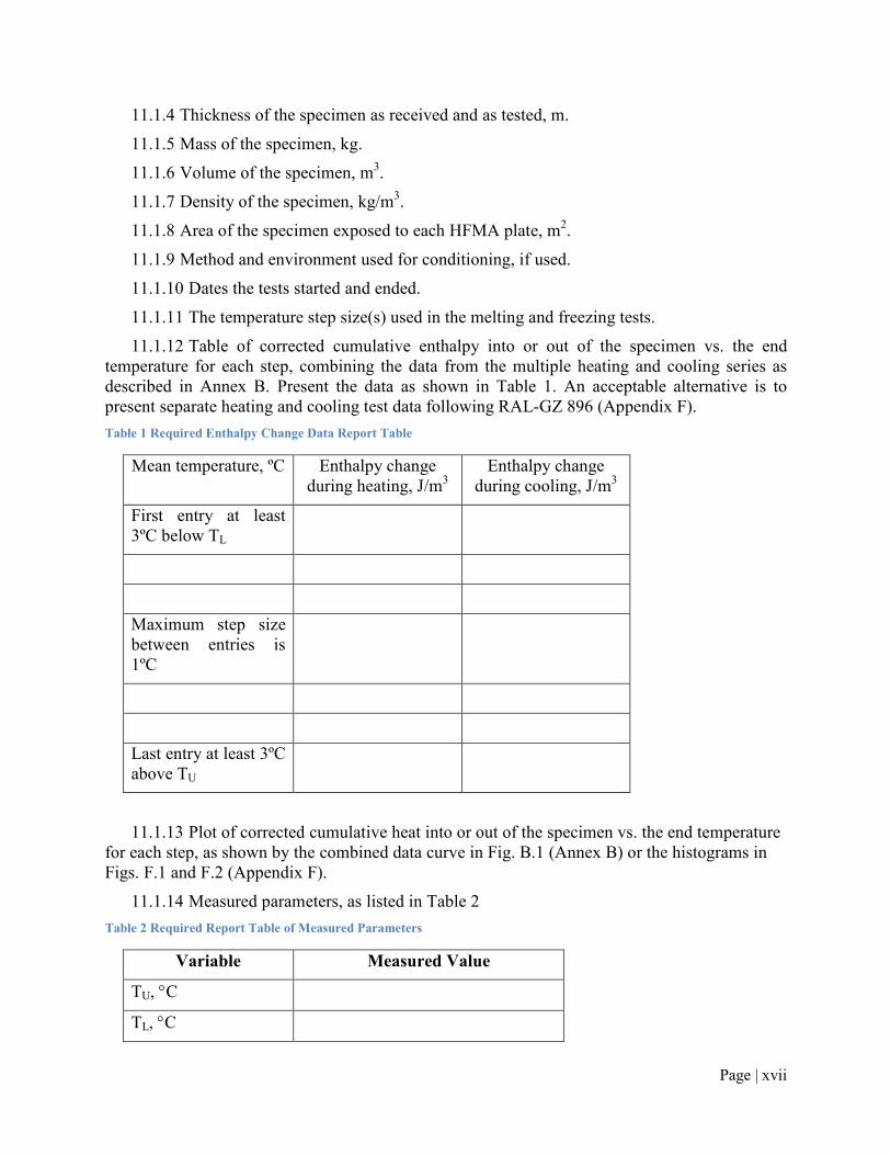
11.1.12 Table of corrected cumulative enthalpy into or out of the specimen vs. the end

temperature for each step, combining the data from the multiple heating and cooling series as

described in Annex B. Present the data as shown in Table 1. An acceptable alternative is to

present separate heating and cooling test data following RAL-GZ 896 (Appendix F).

Table 1 Required Enthalpy Change Data Report Table

Mean temperature, ºC Enthalpy change

during heating, J/m3

Enthalpy change

during cooling, J/m3

First entry at least

3ºC below TL

Maximum step size

between entries is

1ºC

Last entry at least 3ºC

above TU

11.1.13 Plot of corrected cumulative heat into or out of the specimen vs. the end temperature

for each step, as shown by the combined data curve in Fig. B.1 (Annex B) or the histograms in

Figs. F.1 and F.2 (Appendix F).

11.1.14 Measured parameters, as listed in Table 2

Table 2 Required Report Table of Measured Parameters

Variable Measured Value

TU, °C

TL, °C

Page | xviii

cp,M, J/kg-°C

cp,M, J/kg-°C

hfs,, J/kg

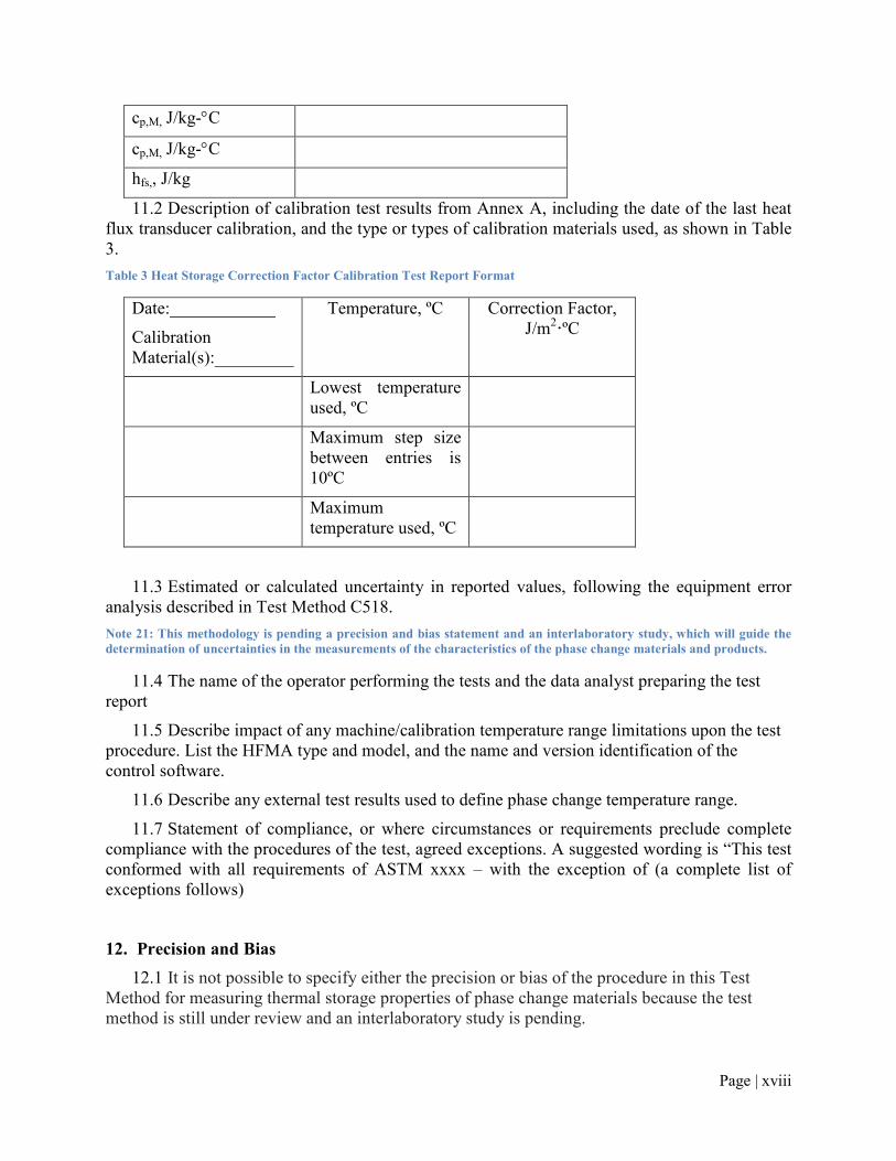
11.2 Description of calibration test results from Annex A, including the date of the last heat

flux transducer calibration, and the type or types of calibration materials used, as shown in Table

3.

Table 3 Heat Storage Correction Factor Calibration Test Report Format

Date:____________

Calibration

Material(s):_________

Temperature, ºC Correction Factor,

J/m2·ºC

Lowest temperature

used, ºC

Maximum step size

between entries is

10ºC

Maximum

temperature used, ºC

11.3 Estimated or calculated uncertainty in reported values, following the equipment error

analysis described in Test Method C518.

Note 21: This methodology is pending a precision and bias statement and an interlaboratory study, which will guide the

determination of uncertainties in the measurements of the characteristics of the phase change materials and products.

11.4 The name of the operator performing the tests and the data analyst preparing the test

report

11.5 Describe impact of any machine/calibration temperature range limitations upon the test

procedure. List the HFMA type and model, and the name and version identification of the

control software.

11.6 Describe any external test results used to define phase change temperature range.

11.7 Statement of compliance, or where circumstances or requirements preclude complete

compliance with the procedures of the test, agreed exceptions. A suggested wording is “This test

conformed with all requirements of ASTM xxxx – with the exception of (a complete list of

exceptions follows)

12. Precision and Bias

12.1 It is not possible to specify either the precision or bias of the procedure in this Test

Method for measuring thermal storage properties of phase change materials because the test

method is still under review and an interlaboratory study is pending.

Page | xix

13. Keywords

13.1 Phase Change Material, Enthalpy Storage, Latent Heat

14. References

1. Gunther, E., Hiebler, S., Mehling, H. and Redlich, R., “Enthalpy of Phase Change

Materials as a Function of Temperature: Required Accuracy and Suitable

Measurement Methods,” International Journal of Thermophysics, Vol. 30, 2009, pp.

1257-1269.

2. Dutil, Y., Rousse, D., Lassue, S., Zalewski, L., Joulin, A., Virgone, J., Kuznik, F.,

Johannes, K., Dumas, J-P., Bédécarrats, J-P., Castell, A. and Cabeza, L.F., “Modeling

phase change materials behavior in building applications: Comments on material

characterization and model validation,” Renewable Energy, 2012 (in press).

3. Kedl, R. J., “Wallboard with Latent Heat Storage for Passive Solar Applications,”

ORNL/TM-11541, Oak Ridge National Laboratory, Oak Ridge, TN, 1991.

4. Stovall, T. K. and Tomlinson, J. J., “ What Are the Potential Benefits of Including

Latent Storage in Common Wallboard?,” Journal of Solar Energy Engineering, Vol.

117, 1995, pp 318-325.

5. Shukla N., Fallahi A. and Kosny J., “Performance characterization of PCM

impregnated gypsum board for building applications,” Proceedings of SHC 2012

Conference, San Francisco, USA, July 2012.

6. Kośny J., Yarbrough D.W., Miller W., Wilkes K. and Lee E., “Analysis of the

Dynamic Thermal Performance of Fiberous Insulations Containing Phase Change

Materials,” Proceedings of the Effstock 2009 - The 11th International Conference on

Thermal Energy Storage, Stockholm, Sweden, June 2009.

7. Kosny J., Kossecka E., Brzezinski B., Tleoubaev A. and Yarbrough D., “Dynamic

Thermal Performance Analysis Of Fiber Insulations Containing Bio-Based Phase

Change Materials (PCMs),” Energy & Buildings, Vol. 52, 2012, pp. 122-131.

8. Kosny J., Stovall T., Shrestha S. and Yarbrough D. “Theoretical and Experimental

Thermal Performance Analysis of Complex Thermal Storage Membrane Containing

Bio-Based Phase-Change Material (PCM)” Thermal Envelopes XI - Thermal

Performance of the Exterior Envelopes of Buildings, Clearwater, Florida, USA,

December 2010.

9. Castellon, C., Gunther, E., Mehling, H., Hiebler, S. and Cabeza, L.F., “Determination

of the enthalpy of PCM as a function of temperature using a heat-flux DSC – A study

of different measurement procedures and their accuracy,” International Journal of

Energy Research, Vol. 32, 2008, pp. 1258-1265.

10. Tleoubaev, A. Brzezinski, A. and Braga, L., “Accurate Simultaneous Measurements

of Thermal Conductivity and Specific Heat of Rubber, Elastomers, and Other

Materials,” 12th

Brazilian Rubber Technology Congress, 2008.

Page | xx

11. Smith, S.E., Stovall, T.K. and Childs, K., “Development of a Dynamic Heat flow

Meter Testing Protocol,” Thermal Conductivity 31/Thermal Expansion 19:

Proceedings of the 31st International Thermal Conductivity Conference and the 19th

International Thermal Expansion Symposium, Montagnais, Canada, June 2011.

12. Zhang, Y., Jiang, Y. and Jiang, Y., “A simple method, the T-history method, of

determining the heat of fusion, specific heat and thermal conductivity of phase-

change materials. Measurement Science and Technology, Vol. 10, 1999, pp. 201–205.

13. Lazaro, A., Gunther, E., Mehling, H., Hiebler, S., Marın, J.M. and Zalba, B.,

“Verification of a T-history installation to measure enthalpy versus temperature

curves of phase change materials,” Measurement Science and Technology, Vol. 17,

2006, pp. 2168–2174.

ANNEXES

(Mandatory Information)

A. Calculation of Correction Factors

A.1. The heat flux levels obtained during an HFMA test run are, in general, determined by heat

flowing into or out of the sample, but also by heat that enters or leaves the HFTs themselves,

due to a change of the transducer temperature. Such heat flow is incidental to the values used

in characterizing the PCM product, and the magnitude of the heat flow must be determined

separately by conducting a heat storage correction factor calibration of the HFMA’s heat flux

transducers.

A1.1 This calibration shall be performed once for each apparatus, using the test procedure

based on Tleoubaev et al. (9).

A1.2 The correction factor is not equal to the specific heat of the transducers themselves

because the temperature profile through the transducer thickness is not linear until the

temperature within the apparatus plate has reached steady state. Therefore the electrical output of

the transducers is not directly proportional to the heat flowing into the transducers during this

time period (11).

A1.3 If any other material is placed between the HFMA plates and the test specimen, the

same type of correction must be made.

A.2. The apparatus heat flux transducer correction factor calibration must be performed over

the entire temperature range in which PCM products will be tested, using an incremental

temperature step procedure:

A2.1 Use two or more specimens of the same material with a known and small heat capacity

in the HFMA chamber to provide data at multiple plate separation values.

Note A.1: Multiple thin boards of well-aged extruded polystyrene, 10 mm each, have been used for this purpose.

A2.2 Starting at the lowest expected temperature and ending at the highest expected

temperature, make a series of measurements as described in 9.3, with the temperature difference

between setpoints of approximately 10ºC, recording readings of heat flux.

Page | xxi

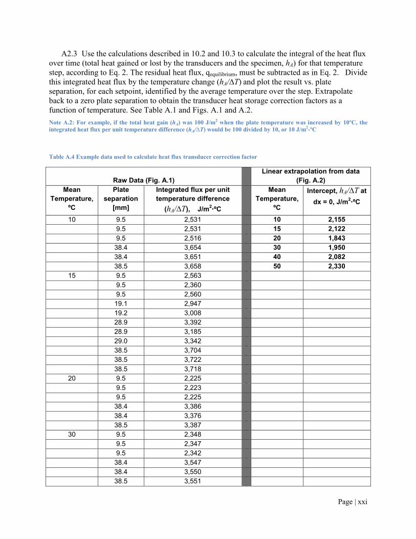
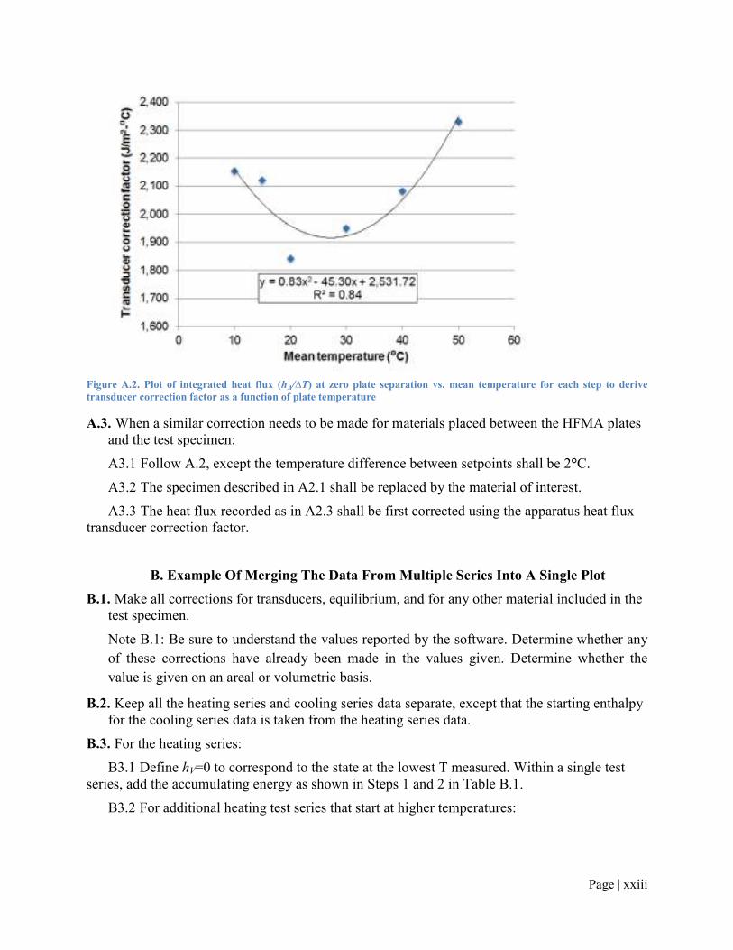
A2.3 Use the calculations described in 10.2 and 10.3 to calculate the integral of the heat flux

over time (total heat gained or lost by the transducers and the specimen, hA) for that temperature

step, according to Eq. 2. The residual heat flux, qequilibrium, must be subtracted as in Eq. 2. Divide

this integrated heat flux by the temperature change (hA/∆T) and plot the result vs. plate

separation, for each setpoint, identified by the average temperature over the step. Extrapolate

back to a zero plate separation to obtain the transducer heat storage correction factors as a

function of temperature. See Table A.1 and Figs. A.1 and A.2.

Note A.2: For example, if the total heat gain (hA) was 100 J/m2 when the plate temperature was increased by 10ºC, the

integrated heat flux per unit temperature difference (hA/∆T) would be 100 divided by 10, or 10 J/m2-ºC

Table A.4 Example data used to calculate heat flux transducer correction factor

Raw Data (Fig. A.1)

Linear extrapolation from data

(Fig. A.2)

Mean

Temperature,

ºC

Plate

separation

[mm]

Integrated flux per unit

temperature difference

(hA/∆T), J/m2∙ºC

Mean

Temperature,

ºC

Intercept, hA/∆T at

dx = 0, J/m2∙ºC

10 9.5 2,531 10 2,155

9.5 2,531 15 2,122

9.5 2,516 20 1,843

38.4 3,654 30 1,950

38.4 3,651 40 2,082

38.5 3,658 50 2,330

15 9.5 2,563

9.5 2,360

9.5 2,560

19.1 2,947

19.2 3,008

28.9 3,392

28.9 3,185

29.0 3,342

38.5 3,704

38.5 3,722

38.5 3,718

20 9.5 2,225

9.5 2,223

9.5 2,225

38.4 3,386

38.4 3,376

38.5 3,387

30 9.5 2,348

9.5 2,347

9.5 2,342

38.4 3,547

38.4 3,550

38.5 3,551

Page | xxii

40 9.5 2,493

9.5 2,489

9.5 2,488

38.4 3,740

38.4 3,728

38.5 3,723

50 9.5 2,756

9.5 2,763

9.5 2,761

38.4 4,116

38.4 4,017

38.5 4,068

Figure A.1. Plot of raw data to visualize extrapolation of integrated heat flux (hA/∆T) to plate separation of zero

Page | xxiii

Figure A.2. Plot of integrated heat flux (hA/∆T) at zero plate separation vs. mean temperature for each step to derive

transducer correction factor as a function of plate temperature

A.3. When a similar correction needs to be made for materials placed between the HFMA plates

and the test specimen:

A3.1 Follow A.2, except the temperature difference between setpoints shall be 2°C.

A3.2 The specimen described in A2.1 shall be replaced by the material of interest.

A3.3 The heat flux recorded as in A2.3 shall be first corrected using the apparatus heat flux

transducer correction factor.

B. Example Of Merging The Data From Multiple Series Into A Single Plot

B.1. Make all corrections for transducers, equilibrium, and for any other material included in the

test specimen.

Note B.1: Be sure to understand the values reported by the software. Determine whether any

of these corrections have already been made in the values given. Determine whether the

value is given on an areal or volumetric basis.

B.2. Keep all the heating series and cooling series data separate, except that the starting enthalpy

for the cooling series data is taken from the heating series data.

B.3. For the heating series:

B3.1 Define hV=0 to correspond to the state at the lowest T measured. Within a single test

series, add the accumulating energy as shown in Steps 1 and 2 in Table B.1.

B3.2 For additional heating test series that start at higher temperatures:

Page | xxiv

B3.2.1 If the previous series included a value at the initial temperature for this series, set the

Cumulative Enthalpy Stored equal to that value, as shown in Step 3 in Table B.1. Continue

through that series using Step 2.

B3.2.2 If the previous series did not include a value at the initial temperature for this series,

interpolate from the previous data, as shown in Step 4 in Table B.1. Continue through that series

using Step 2.

B.4. For the cooling series:

B4.1 Define hV =0 to correspond to the state at the lowest T measured during the heating

series. Select the cooling series that starts from the highest temperature. Use the highest

temperature(s) in the heating series to determine the starting cumulative enthalpy for that cooling

series. Within a single test series, subtract the absolute values of the accumulating energy as

shown in Steps 1 and 2 in Table B.1

B4.2 For additional cooling test series that start at lower temperatures:

B4.2.1 If the previous cooling series included a value at the initial temperature for this series,

set the Cumulative Enthalpy Stored equal to that value, as shown in Step 3 in Table B.1.

Continue through that series using Step 2.

B4.2.2 If the previous series did not include a value at the initial temperature for this series,

interpolate from the previous data, as shown in Step 4 in Table B.1. Continue through that series

using Step 2.

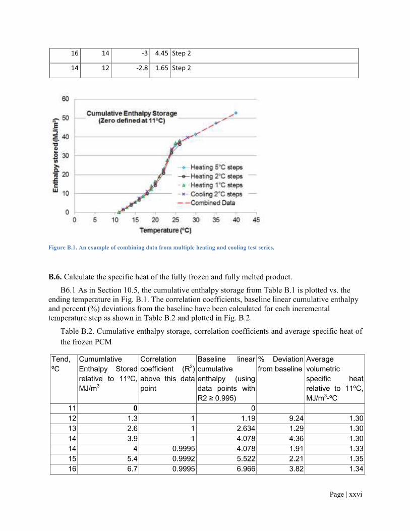
B.5. Plot the data to see if it makes sense, as shown in Fig. B.1. In this example, the heating and

cooling lines were nearly the same. That is not be the case for many PCM products.

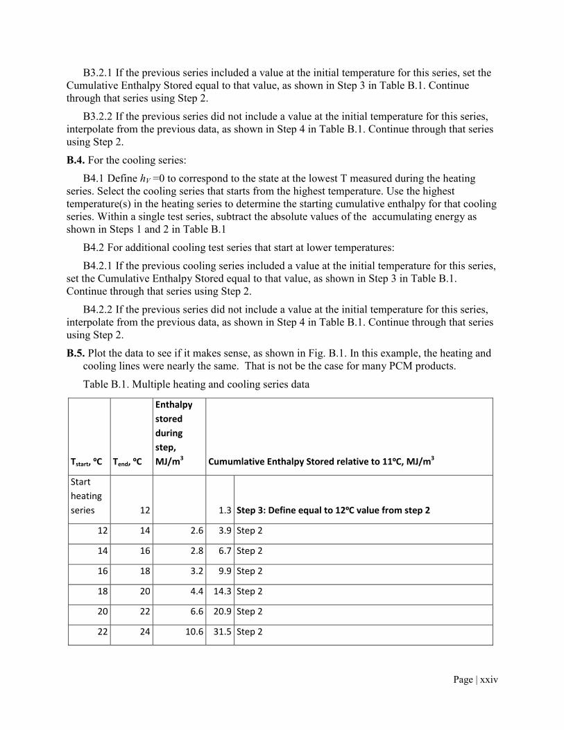
Table B.1. Multiple heating and cooling series data

Tstart, ºC Tend, ºC

Enthalpy

stored

during

step,

MJ/m3 Cumumlative Enthalpy Stored relative to 11ºC, MJ/m

3

Start

heating

series 12

1.3 Step 3: Define equal to 12ºC value from step 2

12 14 2.6 3.9 Step 2

14 16 2.8 6.7 Step 2

16 18 3.2 9.9 Step 2

18 20 4.4 14.3 Step 2

20 22 6.6 20.9 Step 2

22 24 10.6 31.5 Step 2

Page | xxv

24 26 4.8 36.3 Step 2

Start

heating

series 11

0

Step 1: Select Lowest temperature in series,

B3.1 Define cumulative enthalpy storage equal to 0

11 12 1.3 1.3

Step 2: =previous value + enthalpy stored for this

temperature step

12 13 1.3 2.6 Step 2

13 14 1.4 4 Step 2

14 15 1.4 5.4 Step 2

15 16 1.4 6.8 Step 2

16 17 1.6 8.4 Step 2

17 18 1.9 10.3 Step 2

18 19 1.8 12.1 Step 2

18 19 1.9 14 Step 2

19 20 2.3 16.3 Step 2

20 21 2.8 19.1 Step 2

21 22 3.7 22.8 Step 2

22 23 4.8 27.6 Step 2

23 24 5.6 33.2 Step 2

24 25 3.6 36.8 Step 2

25 26 1.2 38 Step 2

Start

cooling

series 28

39.65

Step 4: Set equal to value interpolated between 26 and

30ºC during the heating series

28 26 -2.4 37.25 Step 2

26 24 -3.6 33.65 Step 2

24 22 -11.4 22.25 Step 2

22 20 -6.8 15.45 Step 2

20 18 -4.4 11.05 Step 2

18 16 -3.6 7.45 Step 2

Page | xxvi

16 14 -3 4.45 Step 2

14 12 -2.8 1.65 Step 2

Figure B.1. An example of combining data from multiple heating and cooling test series.

B.6. Calculate the specific heat of the fully frozen and fully melted product.

B6.1 As in Section 10.5, the cumulative enthalpy storage from Table B.1 is plotted vs. the

ending temperature in Fig. B.1. The correlation coefficients, baseline linear cumulative enthalpy

and percent (%) deviations from the baseline have been calculated for each incremental

temperature step as shown in Table B.2 and plotted in Fig. B.2.

Table B.2. Cumulative enthalpy storage, correlation coefficients and average specific heat of

the frozen PCM

Tend,

ºC

Cumumlative

Enthalpy Stored

relative to 11ºC,

MJ/m3

Correlation

coefficient (R2)

above this data

point

Baseline linear

cumulative

enthalpy (using

data points with

R2 ≥ 0.995)

% Deviation

from baseline

Average

volumetric

specific heat

relative to 11ºC,

MJ/m3-ºC

11 0 0

12 1.3 1 1.19 9.24 1.30

13 2.6 1 2.634 1.29 1.30

14 3.9 1 4.078 4.36 1.30

14 4 0.9995 4.078 1.91 1.33

15 5.4 0.9992 5.522 2.21 1.35

16 6.7 0.9995 6.966 3.82 1.34

Page | xxvii

16 6.8 0.9994 6.966 2.38 1.36

17 8.4 0.9985 8.41 0.12 1.40

18 9.9 0.9982 9.854 0.47 1.41

18 10.3 0.9963 9.854 4.53 1.47

19 12.1 0.9943 11.298 7.10

19 14 0.9738 11.298 23.92

20 14.3 0.978 12.742 12.23

20 16.3 0.9687 12.742 27.92

21 19.1 0.9606 14.186 34.64

22 20.9 0.9624 15.63 33.72

22 22.8 0.9557 15.63 45.87

23 27.6 0.9414 17.074 61.65

24 31.5 0.9114 18.518 70.10

24 33.2 0.919 18.518 79.29

25 36.8 0.9145 19.962 84.35

26 36.3 0.9249 21.406 69.58

26 38 0.9352 21.406 77.52

Figure B.2. Cumulative enthalpy storage and correlation coefficients calculated for each incremental temperature step,

which are utilized to determine the average specific heat of a frozen PCM product.

B6.2 The correlation coefficient shows a sharp drop off at T = 19ºC, so the baseline linear

cumulative enthalpy for frozen PCM is plotted using the data points from 11 to 18 ºC. Here, the

percent (%) cumulative enthalpy deviation from the baseline increases over 20% at 19ºC.

Therefore, TL is 18ºC.

B6.2.1 In this particular case, both the correlation coefficient drops below 0.995 and the

percent cumulative enthalpy deviation rises above 20% at 19ºC. When those two occur at

Page | xxviii

different temperatures, TL shall be defined as the temperature above which the percent

cumulative enthalpy deviation rises above 20%

B6.3 For the data points before T=19ºC, the specific heat is the slope of the line, or ~1.44

J/m2∙ºC (average of the two values at T=18ºC).

B6.4 Perform the same exercise, but coming down from the highest temperature to find the

specific heat of the fully melted product and TU. Based on prior experience, the enthalpy storage

curve of the PCM exhibits a sharp transition at the freezing onset (or melting end for heating), so

TU is defined solely by the temperature below which the correlation coefficient drops below

0.995.

APPENDICES

(Nonmandatory Information)

C. History of the Standard

C.1. Experimental measurements were made by Ken Wilkes, David Yarbrough and Jan Kosny to

examine a mixture of cellulose and PCM. These initial efforts were directed toward

determining the impact of the PCM on the thermal conductivity of the mixture, as well as on

determining the PCM enthalpy storage characteristics (6).

C.2. Extensive work has been done in Europe and Asia, as described by Gunther et al. (1),

Castellon et al. (9), Zhang et al. (12), etc. The T-history approach to PCM characterization is

described by Zhang et al. (12) and Lazaro et al. (13).

C2.1 The use of the experimental data to characterize PCM is described in Phase Change

Material Quality Assurance, RAL-GZ 896.

C.3. This modification of the Test Method C518 now used for PCM was initially proposed by

A.Tleoubaev and A.Brzezinski (LaserComp, Inc.) for volumetric specific heat measurements

of regular (i.e. with no PCM) thermal insulation and other materials.

D. Alternate Experimental Approaches

D.1. Not all HFMA machines accommodate a variable gain. However, the amount of energy

flowing through the transducers must be measureable at all points in time. That is, the

transducer output shall never be saturated during a test. Without a variable gain, there are two

ways to ensure this requirement is met.

D1.1 Limit the temperature step size to reduce the heat flow rate to the measurable range.

Consult the manufacturer regarding any accuracy limitations on minimum temperature step size.

D1.2 Insert a thin layer of an insulating material between each side of the specimen and the

apparatus plates to reduce the heat flow rate to the measurable range. The enthalpy storage

correction for the insulating material must be independently measured, in the same manner as for

the HFMA transducers, as described in Annex A. The measured heat flow into the assembly

must then be corrected for this material as described in section 10.

Page | xxix

D.2. Not all HFMA machines allow a zero temperature difference between the plates.

D2.1 One experimental approach has been to use the smallest temperature difference

possible. When stepping to a new temperature condition, both plates will undergo equal

temperature steps and be brought to equilibrium at the new temperatures.

D2.1.1 Under this condition, calculate the net heat flux entering the specimen after the

system has reached steady state. Use an approach similar to that described in 10.1 to correct for

the heat flux due to temperature difference across the specimen.

D2.2 For test specimens with low thermal resistance, place a thin insulating layer between

the specimen and one plate in order to keep the PCM temperature at a nearly uniform

temperature (aside from the temperature gradients that develop in the course of the

melting/freezing process). Measure the temperature on the surface of the PCM product not in

contact with an apparatus plate directly with an auxiliary temperature sensor.

Note D.1: For many such cases the uncertainty in PCM product temperature can be kept

below a few tenths of a Kelvin.

D2.2.1 Corrections shall be made for the heat capacity of the insulating layer, similar to the

plate heat storage correction factor described in Annex A.

E. Explore Hysteresis Effects

E.1. Explore hysteresis effects when starting from partially frozen or partially melted material.

E1.1 Examine the behavior when partially melted material is refrozen. Start at a temperature

2ºC below the lower temperature limit (TL) of the PCM Active Range, as defined in section 10.5.

Use 1.5 +/-0.5ºC steps to reach a temperature midway between TL and TU, as defined in section

10.6. Immediately cool in 1.5 +/-0.5ºC steps until the start temperature is reached.

E1.2 Examine the behavior when partially frozen material is remelted. Start at a temperature

2ºC above the upper temperature limit (TU) of the PCM Active Range, as defined in section 10.6.

Use 1.5 +/-0.5ºC steps to reach a temperature midway between TU and TL, as defined in section

10.5. Immediately heat in 1.5 +/-0.5ºC steps until the start temperature is reached.

E1.3 Evaluate the enthalpy storage as a function of temperature using the method described

in section 10.4 and Annex B.

F. Data Reporting Following RAL-GZ 896

F.1. RAL-GZ 896 requires the specification of stored enthalpy as a function of temperature

separately for the cases of heating and cooling, as there will be differences in the temperature

profile in most cases. It is tabulated in a predetermined temperature range. This must be done in

each case with respect to mass (J/g) and volume (J/m3).

F.2. Figures F.1 and F.2 list the enthalpy storage for each temperature step of the heating and

cooling tests, respectively.

Page | xxx

Figure F.1. Enthalpy stored during a heating test

Figure F.2. Enthalpy stored during a cooling test

T-interval

[°C]

Enthalpy stored

[MJ/m3]

Enthalpy stored

[MJ/g]

12-14 2.6 --

14-16 2.8 --

16-18 3.2 --

18-20 4.4 --

20-22 6.6 --

22-24 10.6 --

24-26 4.8 --

Density at

T °C

--

0

2

4

6

8

10

12

Temperature [°C]

MJ/m3

T-interval

[°C]

Enthalpy stored

[MJ/m3]

Enthalpy stored

[MJ/g]

28-26 -2.4 --

26-24 -3.6 --

24-22 -11.4 --

22-20 -6.8 --

20-18 -4.4 --

18-16 -3.6 --

16-14 -3 --

14-12 -2.8 --

Density at

T °C

--

-12

-10

-8

-6

-4

-2

0

Temperature [°C]

MJ/m3